An XMM-Newton Survey of the Soft X-ray Background. II. An All-Sky Catalog of Diffuse O VII and O VIII Emission Intensities

Abstract

We present an all-sky catalog of diffuse O VII and O VIII line intensities, extracted from archival XMM-Newton observations. This catalog supersedes our previous catalog, which covered the sky between $l=120\arcdeg$ and $l=240\arcdeg$. We attempted to reduce the contamination from near-Earth solar wind charge exchange (SWCX) emission by excluding times of high solar wind proton flux from the data. Without this filtering we were able to extract measurements from 1868 observations. With this filtering, nearly half of the observations became unusable, and only 1003 observations yielded measurements. The O VII and O VIII intensities are typically $\sim$2–11 and $\lesssim$3 photons $\mbox{cm}^{-2}$ $\mbox{s}^{-1}$ $\mbox{sr}^{-1}$ (line unit, L.U.), respectively, although much brighter intensities were also recorded. Our data set includes 217 directions that have been observed multiple times by XMM-Newton. The time variation of the intensities from such directions may be used to constrain SWCX models. The O VII and O VIII intensities typically vary by $\lesssim$5 and $\lesssim$2 L.U. between repeat observations, although several intensity enhancements of $>$10 L.U. were observed. We compared our measurements with models of the heliospheric and geocoronal SWCX. The heliospheric SWCX intensity is expected to vary with ecliptic latitude and solar cycle. We found that the observed oxygen intensities generally decrease from solar maximum to solar minimum, both at high ecliptic latitudes (which is as expected) and at low ecliptic latitudes (which is not as expected). The geocoronal SWCX intensity is expected to depend on the solar wind proton flux incident on the Earth and on the sightline’s path through the magnetosheath. The intensity variations seen in directions that have been observed multiple times are in poor agreement with the predictions of a geocoronal SWCX model. We found that the oxygen lines account for $\sim$40–50% of the 3/4 keV X-ray background that is not due to unresolved active galactic nuclei, in good agreement with a previous measurement. However, we found that this fraction is not easily explainable by a combination of SWCX emission and emission from hot plasma in the halo. We also examined the correlations between the oxygen intensities and Galactic longitude and latitude. We found that the intensities tend to increase with longitude toward the inner Galaxy, possibly due to an increase in the supernova rate in that direction or the presence of a halo of accreted material centered on the Galactic Center. The variation of intensity with Galactic latitude differs in different octants of the sky, and cannot be explained by a single simple plane-parallel or constant-intensity halo model.

1. INTRODUCTION

The soft X-ray background (SXRB) is the diffuse X-ray emission observed in all directions in the $\sim$0.1–10 keV band (McCammon & Sanders, 1990). At energies $\gtrsim$$1~{}\mbox{keV}$, this emission is dominated by unresolved emission from distant active galactic nuclei (AGN; e.g., Brandt & Hasinger 2005). Below $\sim$$1~{}\mbox{keV}$, Galactic line emission becomes important, and dominates at the lowest energies. Some of this line emission comes from hot interstellar gas – possible unabsorbed emission from $\sim$million-degree gas in the Local Bubble (LB; Sanders et al. 1977; Cox & Reynolds 1987; McCammon & Sanders 1990; Snowden et al. 1990; although see also Welsh & Shelton 2009), and emission from $\sim$1–3 million-degree gas in the Galactic halo attenuated by the Galaxy’s H I (Burrows & Mendenhall, 1991; Snowden et al., 1991, 1998, 2000; Wang, 1998; Pietz et al., 1998; Kuntz & Snowden, 2000; Smith et al., 2007; Galeazzi et al., 2007; Henley & Shelton, 2008; Lei et al., 2009; Yoshino et al., 2009; Gupta et al., 2009; Henley et al., 2010).

In addition to the emission from hot interstellar gas, X-ray line emission is produced within our solar system, as a consequence of charge exchange reactions between solar wind ions and neutral hydrogen and helium atoms. Solar wind charge exchange (SWCX) reactions can occur in the heliosphere between solar wind ions and neutral hydrogen and helium atoms that have entered the heliosphere from interstellar space (e.g., Cravens, 2000; Robertson & Cravens, 2003a; Koutroumpa et al., 2006). It can also occur in the Earth’s exosphere, beyond the magnetopause, between solar wind ions and geocoronal neutral hydrogen atoms (e.g. Robertson & Cravens, 2003b). Charge exchange reactions can also occur in the atmospheres of other planets and around comets (e.g., Cravens, 2002; Wargelin et al., 2008), but the resulting emission is sufficiently localized as to not affect the XMM-Newton data set. The heliospheric emission is in general much brighter than the geocoronal emission, although the geocoronal and/or near-Earth heliospheric SWCX emission can exhibit bright enhancements on timescales of $\sim$hours–days, often in association with variations in the solar wind (Cravens et al., 2001; Snowden et al., 2004; Fujimoto et al., 2007; Carter & Sembay, 2008; Carter et al., 2010; Ezoe et al., 2010, 2011). Longer-term variations in SWCX line intensities, on timescales of $\sim$days–years, have also been observed (Koutroumpa et al., 2007; Kuntz & Snowden, 2008; Henley & Shelton, 2008, 2010). These variations may include variations in the global heliospheric SWCX emission, which is expected to vary slowly with the solar cycle (Robertson & Cravens, 2003a; Koutroumpa et al., 2006), as well as variations in the geocoronal and near-Earth heliospheric emission. In general it is difficult to disentangle these various effects. From the point of view of someone interested in the hot Galactic gas, the SWCX emission is a time-varying contaminant of the SXRB emission.

The SXRB has been surveyed several times with rocket- and satellite-borne proportional counters (McCammon et al., 1983; Marshall & Clark, 1984; Garmire et al., 1992; Snowden et al., 1997). While the data from these surveys were essential to establishing our current picture of the SXRB and the hot interstellar medium (ISM), these data are of rather low spectral resolution ($E/\Delta E\sim 1$–3). The CCD cameras on board Chandra, XMM-Newton, and Suzaku offer the ability for higher-resolution spectroscopy (e.g., $E/\Delta E\sim 15$ at 1 keV for the XMM-Newton EPIC-MOS). With these cameras, some emission features in SXRB spectra can be resolved, allowing one to measure SWCX emission line strengths (Wargelin et al., 2004; Snowden et al., 2004; Fujimoto et al., 2007; Henley & Shelton, 2008, 2010; Koutroumpa et al., 2009a, 2011; Carter et al., 2010; Ezoe et al., 2011) or the temperature of the halo plasma (Smith et al., 2007; Galeazzi et al., 2007; Henley & Shelton, 2008; Lei et al., 2009; Yoshino et al., 2009; Gupta et al., 2009; Henley et al., 2010).

Prior to this project, CCD-resolution spectra of the SXRB had been presented for only a few tens of directions. In order to greatly increase the number of directions for which good-quality SXRB spectra are available, we have carried out a survey of the SXRB using archival data from the EPIC-MOS cameras (Turner et al., 2001) on board XMM-Newton (Jansen et al., 2001). A key aspect of this survey is that we do not use only blank-sky observations. Any observation in which the target source is not too bright or too extended can potentially be used – the target source is excised, and an SXRB spectrum extracted from the remainder of the field. The first results from this survey were published in Henley & Shelton (2010, hereafter Paper I). We presented SXRB O VII and O VIII intensities extracted from 590 XMM-Newton observations between $l=120\arcdeg$ and $l=240\arcdeg$ (i.e., one third of the sky). We concentrated on these lines as they dominate the Galactic SXRB emission in the XMM-Newton bandpass (McCammon et al., 2002). Their intensities showed considerable variation over the sky, emphasizing the importance of extracting SXRB spectra for as many directions as possible. Here, we complete our survey and present an all-sky catalog of SXRB O VII and O VIII intensities, comprising measurements from 1880 XMM-Newton observations. Note that, in the course of completing our survey, we have completely reprocessed the observations that featured in Paper I. We also now include estimates of the systematic errors associated with our spectral analysis. The current catalog therefore supersedes, rather than supplements, Paper I.

The goal of this survey is to improve our understanding of the hot gas in our Galaxy. We have already made progress in this direction by comparing spectra from Paper I with the predictions of various physical models (Henley et al., 2010). These observations favor a Galactic fountain origin for the hot halo gas, in which gas is driven from the disk into the halo by supernovae (SNe; Shapiro & Field 1976; Bregman 1980; Joung & Mac Low 2006). This new, larger data set will allow us to further test halo models, and investigate how the halo emission varies over the sky. In addition, our survey includes 217 sightlines for which there are multiple observations, separated in time by days to years. In a given direction, any variation in the observed SXRB spectrum is due to variation in the SWCX emission. Hence, a set of observations of the same direction can be used to constrain SWCX models, which are essential for obtaining accurate spectra of the hot Galactic gas from SXRB observations.

The remainder of this paper is arranged as follows. In Section 2 we outline the data processing (see Paper I for more details). In Section 3 we present our oxygen intensity measurements. We discuss our results in Section 4. In particular, in Section 4.1 we discuss the implications of our results for SWCX. In Section 4.2 we discuss the oxygen lines’ contribution to the 3/4 keV SXRB, and the implications for the sources of the SXRB emission. In Section 4.3 we discuss the spatial variation of the oxygen intensities, and the implications of these results for the halo. We summarize our results in Section 5.

2. DATA REDUCTION

The data reduction procedure is described in full in Paper I, to which the reader is referred for more details. Here, we outline the main steps, and also point out any differences from Paper I. The results presented here were obtained from data reduced with the XMM-Newton Science Analysis System (SAS) version 11.0.1, which includes the XMM-Newton Extended Source Analysis Software (XMM-ESAS; Kuntz & Snowden 2008; Snowden & Kuntz 2011). However, much of the preliminary inspection of the data (e.g., for identifying unusable CCDs and for determining source exclusion regions; see below) was carried out on data processed with earlier versions of SAS. Although the latest version of XMM-ESAS can process data from the EPIC-pn camera (Strüder et al., 2001), it only became available after the current data processing was well under way, and so we consider only EPIC-MOS data here.

We used the XMM-ESAS calibration files that were current as of 2011 April 01. After we had completed most of the processing, we learned that these files had been superseded. We reprocessed a random subset of our observations with the newer calibration files (released on 2011 May 16), and found that the effect on our oxygen intensity measurements was not significant, compared with the statistical and systematic uncertainties. We therefore decided not to reprocess our entire data set with the newer calibration files.

2.1. Observation Selection and Initial Data Processing

As of 2010 August 04, there were 5698 publicly available XMM-Newton observations with at least some MOS exposure. We processed each observation with the SAS emchain script, excluding observations that had been rejected in Paper I due to obvious contamination from soft protons impinging upon the detector, or due to bright or extended sources in the field of view. This script produces a calibrated events list for each MOS exposure. We then used the XMM-ESAS mos-filter script to identify and remove times affected by soft-proton flaring. For each events list, this script creates a histogram of count-rates from the 2.5–12 keV light curve, using 60-s bins, fits a Gaussian to the peak of this histogram, and rejects all times whose count-rates differ by more than 1.5$\sigma$ from the mean of the Gaussian. (Although there are some superficial differences here from the description in Paper I, these are solely due to changes in the way XMM-ESAS is organized. These first steps in the processing are essentially identical to those used in Paper I.)

We discarded all exposures that did not have at least 5 ks of good time after the above filtering, and then discarded any observation that did not have at least one good MOS1 exposure and at least one good MOS2 exposure. We then inspected the light curves and histograms of count-rates produced by mos-filter, checking for observations that were badly affected by soft protons, but for which mos-filter yielded $\geq$5 ks of good time. Such observations are generally apparent from the non-Gaussianity of the histogram of count-rates. Figure 1 shows an example – despite the clear soft-proton contamination, mos-filter yielded $\approx$12 ks of good time for this observation. Observations like this were rejected.

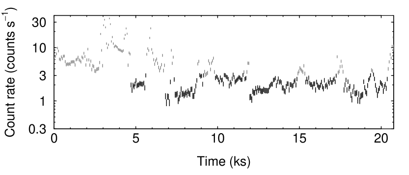
Figure 1.— Histogram of MOS1 count-rates (top) and MOS1 light curve (bottom) for the 2.5–12 keV band, from obs. 0051760201 (an observation for which mos-filter yielded $\geq$5 ks of good time, despite the presence of severe soft-proton contamination). The curve in the upper panel is the Gaussian that was fitted to the histogram of count-rates. Times whose count-rates differed by more than 1.5$\sigma$ from the mean of this Gaussian were rejected; such times are plotted in gray in the lower panel.

For each remaining observation, we examined the cleaned images produced by mos-filter. Because our ultimate goal was to extract SXRB spectra, we rejected observations whose fields contained large diffuse sources (e.g., galaxy clusters) that filled all or most of the field of view, or very bright sources for which the emission in the wings of the point spread function (PSF) would dominate over the SXRB emission. We also rejected observations that exhibited bright arcs in the field of view, due to stray-light X-rays from a bright source outside the field of view. The above-described rejections reduced the original set of 5698 observations to 2611, a 54% attrition rate (somewhat higher than the $\sim$45% rate in Paper I).

2.2. Removal of Bright or Extended Sources, and of Unusable CCDs

The visual inspection of the cleaned images served two further purposes. We identified bright and/or extended sources that would not be adequately excised by the automated point source removal procedure described in Section 2.3, below. Such sources were removed using circular exclusion regions. These regions were generally positioned by eye, although if the source to be excluded was the observation target, we used the pointing direction from the events list header to center the exclusion region. The radii of these regions were also chosen by eye, although for some sources we used the radial surface brightness profile to aid us. As noted in Paper I, we erred on the side of choosing larger exclusion radii, at the expense of reducing the number of counts in the SXRB spectra.

The final purpose of the visual inspection of the images was to identify CCDs that should be ignored in the subsequent processing. We ignored CCDs that were in window mode, CCDs that were missing from the images (e.g., the MOS1-6 CCD after its failure in 2005 March), and CCDs that clearly exhibited the anomalous state identified by Kuntz & Snowden (2008) – such CCDs appear unusually bright in a soft-band (0.2–0.9 keV) X-ray image.

2.3. Automated Source Removal

In Paper I, we ran the SAS edetect_chain script on each observation to automatically identify point sources for removal. Here, we instead used data from the Second XMM-Newton Serendipitous Source Catalogue (2XMM; Watson et al. 2009), specifically the 2XMMi DR3 data release. The advantage of using 2XMM data for the automated source removal is that it means that exactly the same point sources are removed from a set of observations of the same direction, which is not guaranteed if the source detection is run on an observation-by-observation basis.

For each observation, we removed all the sources listed in the catalog within the field of view with 0.5–2.0 keV fluxes $F_{\mathrm{X}}^{0.5-2.0}\geq 5\times 10^{-14}~{}\mbox{erg}\ \mbox{cm}^{-2}\ \mbox{s}^{-1}$, determined by combining the fluxes for 2XMM bands 2 and 3. This is the same flux level to which sources were removed in Paper I; this flux threshold was originally chosen because it is the approximate level to which Chen et al. (1997) removed sources when they determined the spectrum of the extragalactic background that we used in the Paper I spectral analysis. However, as described in Section 3.1, below, we used a slightly different model for modeling the extragalactic background in this paper.

We used circles of radius 50″ to excise the above-detected sources. Such source exclusion regions enclose $\approx$90% of each source’s flux (calculated from the best-fit King profiles to the MOS telescopes’ PSFs; see the XMM-Newton Calibration Access and Data Handbook). Note that, in Paper I, we used the SAS region task to define regions that enclosed 90% of each source’s flux. However, this task uses a more centrally peaked model of the PSF than the King profile, and thus appears to underestimate the required source exclusion radii (30″–40″, versus $\approx$50″).

2.4. Reducing SWCX Contamination

In an attempt to reduce the contamination from SWCX produced near the Earth, we removed the portions of the XMM-Newton data taken when the solar wind proton flux exceeds $2\times 10^{8}$ $\mbox{cm}^{-2}$ $\mbox{s}^{-1}$ (see Paper I). As in Paper I, we used data from OMNIWeb, which combines in situ solar wind measurements from several satellites. The data that we used are mainly from the Advanced Composition Explorer (ACE) and Wind. The data from OMNIWeb for these satellites have been time-shifted to the Earth. The OMNIWeb data covering the XMM-Newton mission also include data from near-Earth satellites that are not time-shifted, but this lack of time-shifting should not adversely affect our results (see Paper I).

As noted in Paper I, this filtering by solar wind proton flux resulted in, for some observations, the amount of usable observation time falling below our 5 ks threshold (see Section 2.1). After carrying out this filtering, the number of usable observations fell from 2611 to 1435. Below, we present the results obtained both with and without this filtering.

Although this proton flux filtering is the only step that we take during our data processing that is aimed at reducing SWCX contamination, we also take steps during our post-processing analysis aimed at culling contaminated observations. For this, we take advantage of the results of Carter et al. (2011), who describe a method for identifying XMM-Newton observations that are contaminated by SWCX emission (see also Carter & Sembay 2008). An observation is identified as SWCX-contaminated if it exhibits variation in a narrow energy band spanning the O VII and O VIII lines that is uncorrelated with variation in a higher-energy continuum-dominated band. This method is sensitive in particular to geocoronal SWCX emission that varies significantly during the course of an observation.

Rather than trying to emulate the Carter et al. method, we will make use of Table A.1 in Carter et al. (2011), which identifies 103 XMM-Newton observations affected by geocoronal SWCX. When we present our oxygen intensity measurements in Section 3.3, below, we will compare the intensities extracted from the observations flagged by Carter et al. (2011) with those extracted from our survey as a whole. Later, in Section 4, we will discuss various aspects of our results. In certain cases, it will be desirable to reduce the effects of SWCX contamination on our results. In such cases, we will exclude the observations identified by Carter et al. (2011) as SWCX-contaminated, and will make it clear whether or not we are doing so.

2.5. Spectra, Response Files, and Particle Background

For each exposure of each observation, we extracted an SXRB spectrum from the full field of view, minus any excluded sources or CCDs. We extracted the spectra using the XMM-ESAS mos-spectra script. This script also created the redistribution matrix files (RMFs) and ancillary response files (ARFs), using the SAS rmfgen and arfgen tasks, respectively. Note that, because we extract the SXRB spectra from the full field of view, our survey is insensitive to structure in the SXRB on scales smaller than $\sim$0.5°. Our sensitivity to SXRB structure on larger scales depends on the location of the archival XMM-Newton observations on the sky, and on our ability to remove the time-variable SWCX contamination.

The extracted spectra consist of the true SXRB emission (including SWCX, Galactic, and extragalactic emission), the quiescent particle background (QPB), and residual contamination from soft protons impinging upon the detector that remains despite the cleaning of the data by mos-filter. For each extracted spectrum, we subtracted the QPB spectrum, which we calculated using the XMM-ESAS mos_back program. The QPB spectra were constructed from a database of filter-wheel-closed data, scaled using data from the regions of the MOS detector outside the field of view (see Kuntz & Snowden 2008 for details). We dealt with the residual soft-proton contamination by including an extra model component in the spectral analysis (see Section 3.1, below).

As noted in Section 2.2, we ignored CCDs that clearly exhibited the anomalous state identified by Kuntz & Snowden (2008). However, it was not always possible to clearly identify anomalous CCDs from a visual inspection of the X-ray images. Originally, we used plots of hardness ratio against count-rate for the unexposed corner pixels (which are produced by the above-described processing) to identify previously unidentified anomalous CCDs (see Paper I). However, the latest version of mos_back (included in SAS version 11.0.1) fails if it identifies a CCD in an anomalous state (for some observations, mos_back identified anomalous CCDs that we had failed to identify in Paper I). In either case, if a CCD was identified as being in an anomalous state, we ignored that CCD, and re-ran the spectral extraction and QPB calculation for the observation in question.

3. OXYGEN LINE INTENSITIES

In this section we present our SXRB oxygen intensity measurements. We describe our methods for measuring the oxygen line intensities and for estimating the systematic errors in Sections 3.1 and 3.2, respectively. The main set of results is presented in Section 3.3, while in Section 3.4 we present results for directions that have multiple usable XMM-Newton observations. In the subsequent subsections we discuss any differences in our new results from those in Paper I, the possibility of contamination from bright sources and from soft protons, the effect of the proton flux filtering described in Section 2.4, and the sky coverage of our survey.

3.1. Measurement Method

We measured the oxygen line intensities using XSPEC version 12.7.0. The method that we used is almost identical to that used in Paper I. The differences are how we modeled the extragalactic background, and how we modeled the residual soft-proton contamination (see below). We now also include estimates of the systematic errors associated with some of our spectral model assumptions (see Section 3.2, below).

For each observation, we fitted a multicomponent spectral model simultaneously to the 0.4–10.0 keV QPB-subtracted spectra extracted from the usable exposures (in most cases, there was one MOS1 spectrum and one MOS2 spectrum). This model included two $\delta$-functions to model the O VII and O VIII K$\alpha$ emission. The O VII line energy was a free parameter, while the O VIII energy was fixed at 0.6536 keV (from APEC; Smith et al. 2001). This method measures the total observed oxygen line intensities, including foreground SWCX and/or LB emission, and attenuated halo emission, in photons $\mbox{cm}^{-2}$ $\mbox{s}^{-1}$ $\mbox{sr}^{-1}$ (hereafter referred to as line units, L.U.). The remaining Galactic line emission was modeled with an absorbed APEC thermal plasma model (Smith et al., 2001) with the oxygen K$\alpha$ emission disabled (see Lei et al. 2009). We also tried other spectral codes, to estimate the size of the systematic error associated with our choice of code (see Section 3.2, below). The extragalactic background was modeled with an absorbed power-law with a photon index of 1.46 (Chen et al. 1997; see below for discussion of this component’s normalization). From here on we refer to this component as the extragalactic power-law (EPL). The APEC and EPL components were attenuated using the XSPEC phabs model (Bałucińska-Church & McCammon, 1992; Yan et al., 1998), with the absorbing column $N_{\mathrm{H}}$ fixed at the H I column density from the LAB H I survey (Kalberla et al., 2005) for the direction of the XMM-Newton observation being analyzed. The model also included two Gaussians to model the bright Al-K and Si-K instrumental lines at 1.49 and 1.74 keV (Kuntz & Snowden, 2008). See Paper I for more details about these model components. We used Anders & Grevesse (1989) abundances for the APEC and phabs model components.

It is possible that, despite the cleaning described in Section 2, some contamination from soft protons impinging upon the detector will remain in the extracted spectra. This contamination manifests itself as excess emission over the EPL at higher energies. Following advice in the XMM-ESAS manual (Snowden & Kuntz, 2011), we modeled this residual contamination by adding a power-law that was not folded through the instrumental response to the above-described model. We set soft limits on the power-law index at 0.5 and 1.0, and hard limits at 0.2 and 1.3. This is in contrast to Paper I, in which we used a broken power-law with a break at 3.2 keV (Snowden & Kuntz, 2007; Kuntz & Snowden, 2008) and no constraints on the spectral indices to model the residual soft-proton contamination. This change appeared to have little effect on the results. The parameters of the soft-proton power-law were independent for each exposure.

The above-described soft-proton contamination makes it difficult to independently constrain the normalization of the EPL, because there is some degeneracy between these two model components at higher energies. In Paper I, we simply fixed the normalization of the EPL at 10.5 photons $\mbox{cm}^{-2}$ $\mbox{s}^{-1}$ $\mbox{sr}^{-1}$ $\mbox{keV}^{-1}$ (throughout this paper, we specify the normalization of the EPL at 1 keV). This value was found by Chen et al. (1997) from a joint ROSAT + ASCA spectrum, after a few sources with $F_{\mathrm{X}}^{0.5-2.0}\gtrsim 5\times 10^{-14}~{}\mbox{erg}\ \mbox{cm}^{-2}\ \mbox{s}^{-1}$ were excised from the data. However, as discussed in Paper I, the X-ray source counts from Moretti et al. (2003) imply that the extragalactic background composed of sources with $F_{\mathrm{X}}^{0.5-2.0}<5\times 10^{-14}~{}\mbox{erg}\ \mbox{cm}^{-2}\ \mbox{s}^{-1}$ should have a lower normalization than this. The integrated 0.5–2.0 keV surface brightness due to sources with $F_{\mathrm{X}}^{0.5-2.0}<5\times 10^{-14}~{}\mbox{erg}\ \mbox{cm}^{-2}\ \mbox{s}^{-1}$ is $5.46\times 10^{-12}~{}\mbox{erg}\ \mbox{cm}^{-2}\ \mbox{s}^{-1}\ \mathrm{deg}^{-2}$ (Moretti et al., 2003). Assuming a photon index of 1.46 (Chen et al., 1997), this surface brightness implies a normalization for the EPL of 7.9 photons $\mbox{cm}^{-2}$ $\mbox{s}^{-1}$ $\mbox{sr}^{-1}$ $\mbox{keV}^{-1}$ (Paper I). In this paper, we used this lower value as the nominal value for the normalization of the EPL.

To allow for field-to-field variation in the number of unresolved sources contributing to the extragalactic background, we experimented with allowing the EPL normalization to be a free parameter, with soft limits at $\pm$15% and hard limits at $\pm$30% of the nominal value of 7.9 photons $\mbox{cm}^{-2}$ $\mbox{s}^{-1}$ $\mbox{sr}^{-1}$ $\mbox{keV}^{-1}$. To help break the degeneracy between the EPL and the soft-proton power-law, we increased the upper energy limit for the spectral fitting from 5 keV (Paper I) to 10 keV. This should have helped because the EPL falls off more rapidly than the soft-proton power-law above $\sim$5 keV, owing to the former having been folded through the instrumental response while the latter was not. However, we found that best-fit EPL normalizations had a tendency to cluster near the soft limits, rather than being distributed approximately symmetrically about the nominal value with a peak at the nominal value. We therefore opted to make the oxygen measurements with the EPL normalization fixed at the nominal value. In the following subsection we describe how we estimated the size of the systematic error associated with our assuming this normalization.

3.2. Systematic Errors

We estimated the systematic errors associated with some of the assumptions in our spectral model, specifically, our use of an APEC model for the non-oxygen line emission, and our fixing the EPL normalization at 7.9 photons $\mbox{cm}^{-2}$ $\mbox{s}^{-1}$ $\mbox{sr}^{-1}$ $\mbox{keV}^{-1}$. We include these systematic errors alongside the statistical errors in our tables of results, below. In Paper I, we found that any systematic error associated with our choice of EPL normalization was typically smaller than the statistical error on the intensity, but we did not include estimates of the systematic errors in our tables of results. In Paper I, we also considered contamination by bright sources or by soft protons as possible sources of systematic error – we will discuss these in Section 3.6.

To estimate the systematic error associated with our use of an APEC model for the non-oxygen line emission, we repeated the analysis using a MeKaL model (Mewe et al., 1995) or a Raymond & Smith (1977 and updates) model in place of the APEC model. We disabled the oxygen lines for these models by setting the oxygen abundance in XSPEC to zero. Note that this method disables all oxygen emission from the model plasma, whereas in our original method, described above, we disabled only the oxygen K$\alpha$ emission. This means that, in these new measurements, the O VIII line may be contaminated by emission from O VII K$\beta$ at 0.666 keV. However, as the intensity of the O VII K$\beta$ line relative to the O VIII Ly$\alpha$ line is dependent upon the temperature, which is not always well constrained in our models, it is possible that the O VII K$\beta$ emission is not accurately accounted for in our original O VIII Ly$\alpha$ measurements either. Therefore, as well as quantifying the differences between spectral codes, this method should give an estimate of the uncertainty in the O VIII Ly$\alpha$ intensity due to the uncertainty in the O VII K$\beta$ contamination.

We measured the oxygen intensities using the three different codes for all of our observations. For each line in each observation, our estimate of the systematic error associated with our choice of spectral code is

$$\sigma_{\mathrm{sys,code}}=\max\big{\{}|I(\mbox{APEC}) - I(\mbox{{MeKaL}})|,$$

$$|I(\mbox{APEC}) - I(\mbox{Raymond-Smith})|\big{\}},$$ (1)

where $I(\mbox{APEC})$ is the intensity measured using the APEC code, etc.

To estimate the systematic error associated with our fixing the normalization of the EPL, we first used a Monte Carlo simulation to estimate the expected field-to-field variation in the number of sources contributing to the extragalactic background, and thus the variation in the flux and normalization of the EPL. Using source counts from Moretti et al. (2003) and assuming a power-law photon index of 1.46 (Chen et al., 1997), we estimated that the EPL normalization should vary by $\pm$0.8 photons $\mbox{cm}^{-2}$ $\mbox{s}^{-1}$ $\mbox{sr}^{-1}$ $\mbox{keV}^{-1}$ ($1\sigma$) from its nominal value of 7.9 photons $\mbox{cm}^{-2}$ $\mbox{s}^{-1}$ $\mbox{sr}^{-1}$ $\mbox{keV}^{-1}$ among our XMM-Newton fields.

We therefore repeated the oxygen measurements for each observation with the EPL normalization fixed at 7.1 and 8.7 photons $\mbox{cm}^{-2}$ $\mbox{s}^{-1}$ $\mbox{sr}^{-1}$ $\mbox{keV}^{-1}$. For each line in each observation, our estimate of the systematic error associated with our fixing the EPL normalization is

$$\sigma_{\mathrm{sys,EPL}}=\max\big{\{}|I(7.9)-I(7.1)|,|I(7.9)-I(8.7)|\big{\}},$$ (2)

where $I(7.9)$ is the intensity measured with the EPL normalization fixed at 7.9 photons $\mbox{cm}^{-2}$ $\mbox{s}^{-1}$ $\mbox{sr}^{-1}$ $\mbox{keV}^{-1}$, etc. We combined $\sigma_{\mathrm{sys,code}}$ and $\sigma_{\mathrm{sys,EPL}}$ in quadrature to get our final estimate of the systematic error, $\sigma_{\mathrm{sys}}$.

3.3. Results

Table 1O VII and O VIII Line Intensities (Without Proton Flux Filtering)

Obs. ID	Start	$l$	$b$	$t^{\mathrm{exp}}_{1}$	$\Omega_{1}$	$t^{\mathrm{exp}}_{2}$	$\Omega_{2}$	$I_{\mathrm{O\,VII}}$	$E_{\mathrm{O\,VII}}$	$I_{\mathrm{O\,VIII}}$	$\langle f_{\mathrm{sw}}\rangle$	$\frac{F_{\mathrm{total}}^{2-5}}{F_{\mathrm{exgal}}^{2-5}}$
	Date	(deg)	(deg)	(ks)	(arcmin2)	(ks)	(arcmin2)	(L.U.)	(keV)	(L.U.)	($10^{8}~{}\mbox{cm}^{-2}~{}\mbox{s}^{-1}$)
(1)	(2)	(3)	(4)	(5)	(6)	(7)	(8)	(9)	(10)	(11)	(12)	(13)
0146390201	2003-03-29	0.005	$-17.799$	17.1	537	17.4	474	$9.72\pm 1.03\pm 1.77$	0.5575	$1.13\pm 0.49\pm 0.60$	8.55	2.43
0050940401	2002-03-14	0.015	$-12.011$	8.4	583	9.2	589	$35.17^{+1.55}_{-2.29}\pm 2.52$	0.5725	$15.68^{+1.16}_{-1.35}\pm 6.78$	1.14	2.64
0402781001	2007-01-20	0.271	$+48.208$	16.1	421	16.0	583	$9.34^{+1.03}_{-1.10}\pm 1.72$	0.5725	$3.61^{+0.65}_{-0.67}\pm 1.39$	1.27	2.41
0021540501	2001-08-26	0.426	$+48.796$	$\cdots$	$\cdots$	$\cdots$	$\cdots$	$\cdots$	$\cdots$	$\cdots$	$\cdots$	$\cdots$
0413780101	2007-02-24	0.604	$+11.378$	23.0	453	23.4	542	$3.29^{+0.96}_{-1.00}\pm 1.09$	0.5675	$2.06^{+0.75}_{-0.48}\pm 0.62$	2.70	1.72
0202190301	2004-05-20	0.939	$-79.578$	16.8	570	17.0	578	$5.71^{+0.89}_{-0.84}\pm 0.18$	0.5675	$1.21^{+0.51}_{-0.46}\pm 0.42$	3.07	2.39
0413780201	2007-03-03	0.960	$+10.788$	25.4	500	25.0	590	$4.77^{+0.87}_{-0.86}\pm 0.56$	0.5775	$4.30^{+0.57}_{-0.58}\pm 1.10$	1.91	1.68
0413780301	2007-03-07	1.168	$+10.439$	16.2	430	16.6	592	$5.98^{+1.26}_{-1.53}\pm 0.42$	0.5725	$4.78^{+0.77}_{-0.86}\pm 0.84$	0.86	2.53
0152750101	2002-09-27	1.540	$+7.099$	38.7	580	39.0	589	$8.43^{+0.40}_{-0.97}\pm 2.48$	0.5625	$6.42^{+0.43}_{-0.31}\pm 1.20$	3.27	2.50
0556210501	2008-07-19	1.649	$+46.606$	10.8	488	10.9	578	$12.01^{+1.67}_{-1.22}\pm 0.94$	0.5675	$3.95^{+0.72}_{-0.71}\pm 1.26$	1.65	1.88
0201903001	2004-10-24	2.718	$-56.160$	17.4	352	17.8	296	$5.97^{+1.51}_{-1.31}\pm 0.38$	0.5725	$0.99^{+0.74}_{-0.75}\pm 0.20$	3.51	2.65
0205390101	2005-05-01	3.588	$-64.104$	27.6	311	27.6	396	$7.40^{+0.90}_{-0.96}\pm 0.49$	0.5675	$1.14^{+0.57}_{-0.51}\pm 0.72$	1.17	2.18
0404910801	2006-05-02	3.966	$-59.441$	19.9	332	19.4	340	$6.27^{+1.87}_{-0.91}\pm 1.22$	0.5675	$0.70^{+0.88}_{-0.57}\pm 1.09$	3.04	1.89
0018741701	2001-05-03	3.967	$-59.448$	6.6	341	6.6	340	$11.29\pm 2.03\pm 1.31$	0.5675	$5.49\pm 1.23\pm 0.55$	2.14	2.18
0135980201	2002-04-30	4.693	$-64.122$	25.5	551	25.8	559	$11.70^{+0.50}_{-0.89}\pm 0.26$	0.5625	$2.77^{+0.42}_{-0.41}\pm 1.28$	2.86	1.65
0148520101	2003-07-22	5.456	$+56.770$	21.6	582	21.3	588	$12.42^{+0.78}_{-0.82}\pm 1.51$	0.5675	$4.47^{+0.47}_{-0.55}\pm 2.52$	1.18	1.74
0057560301	2001-08-09	5.457	$+56.766$	36.6	587	36.1	514	$13.99\pm 0.63\pm 1.11$	0.5675	$4.71\pm 0.39\pm 2.67$	1.77	1.69
0302580501	2005-06-13	5.676	$-77.683$	36.1	394	37.3	481	$8.46^{+1.33}_{-0.73}\pm 0.85$	0.5675	$2.01^{+0.59}_{-0.40}\pm 1.11$	2.10	2.32

Note. — This table is available in its entirety in a machine-readable form in the online journal. A portion is shown here for guidance regarding its form and content.

Table 2O VII and O VIII Line Intensities (With Proton Flux Filtering)

Obs. ID	Start	$l$	$b$	$t^{\mathrm{exp}}_{1}$	$\Omega_{1}$	$t^{\mathrm{exp}}_{2}$	$\Omega_{2}$	$I_{\mathrm{O\,VII}}$	$E_{\mathrm{O\,VII}}$	$I_{\mathrm{O\,VIII}}$	$\langle f_{\mathrm{sw}}\rangle$	$\frac{F_{\mathrm{total}}^{2-5}}{F_{\mathrm{exgal}}^{2-5}}$	Affected by
	Date	(deg)	(deg)	(ks)	(arcmin2)	(ks)	(arcmin2)	(L.U.)	(keV)	(L.U.)	($10^{8}~{}\mbox{cm}^{-2}~{}\mbox{s}^{-1}$)		filtering?
(1)	(2)	(3)	(4)	(5)	(6)	(7)	(8)	(9)	(10)	(11)	(12)	(13)	(14)
0146390201	2003-03-29	0.005	$-17.799$	$\cdots$	$\cdots$	$\cdots$	$\cdots$	$\cdots$	$\cdots$	$\cdots$	$\cdots$	$\cdots$	$\cdots$
0050940401	2002-03-14	0.015	$-12.011$	8.4	583	9.2	589	$35.17^{+1.55}_{-2.29}\pm 2.52$	0.5725	$15.68^{+1.16}_{-1.35}\pm 6.78$	1.14	2.64	N
0402781001	2007-01-20	0.271	$+48.208$	16.1	421	16.0	583	$9.34^{+1.03}_{-1.10}\pm 1.72$	0.5725	$3.61^{+0.65}_{-0.67}\pm 1.39$	1.27	2.41	N
0021540501	2001-08-26	0.426	$+48.796$	11.0	294	11.1	354	$17.58^{+2.02}_{-2.09}\pm 0.92$	0.5675	$6.19^{+1.18}_{-1.21}\pm 1.10$	1.63	2.69	$\cdots$
0413780101	2007-02-24	0.604	$+11.378$	$\cdots$	$\cdots$	$\cdots$	$\cdots$	$\cdots$	$\cdots$	$\cdots$	$\cdots$	$\cdots$	$\cdots$
0202190301	2004-05-20	0.939	$-79.578$	$\cdots$	$\cdots$	$\cdots$	$\cdots$	$\cdots$	$\cdots$	$\cdots$	$\cdots$	$\cdots$	$\cdots$
0413780201	2007-03-03	0.960	$+10.788$	15.0	500	14.8	590	$4.65^{+1.08}_{-1.02}\pm 0.99$	0.5775	$4.44^{+0.75}_{-0.74}\pm 1.33$	1.61	1.64	Y
0413780301	2007-03-07	1.168	$+10.439$	16.2	430	16.6	592	$5.98^{+1.26}_{-1.53}\pm 0.42$	0.5725	$4.78^{+0.77}_{-0.86}\pm 0.84$	0.86	2.53	N
0152750101	2002-09-27	1.540	$+7.099$	12.6	580	12.7	589	$6.11^{+1.14}_{-1.17}\pm 2.80$	0.5625	$5.43^{+0.63}_{-0.64}\pm 1.62$	1.82	2.49	Y
0556210501	2008-07-19	1.649	$+46.606$	10.8	488	10.9	578	$12.01^{+1.67}_{-1.22}\pm 0.94$	0.5675	$3.95^{+0.72}_{-0.71}\pm 1.26$	1.65	1.88	N
0201903001	2004-10-24	2.718	$-56.160$	$\cdots$	$\cdots$	$\cdots$	$\cdots$	$\cdots$	$\cdots$	$\cdots$	$\cdots$	$\cdots$	$\cdots$
0205390101	2005-05-01	3.588	$-64.104$	27.6	311	27.6	396	$7.40^{+0.90}_{-0.96}\pm 0.49$	0.5675	$1.14^{+0.57}_{-0.51}\pm 0.72$	1.17	2.18	N
0404910801	2006-05-02	3.966	$-59.441$	$\cdots$	$\cdots$	$\cdots$	$\cdots$	$\cdots$	$\cdots$	$\cdots$	$\cdots$	$\cdots$	$\cdots$
0018741701	2001-05-03	3.967	$-59.448$	$\cdots$	$\cdots$	$\cdots$	$\cdots$	$\cdots$	$\cdots$	$\cdots$	$\cdots$	$\cdots$	$\cdots$
0135980201	2002-04-30	4.693	$-64.122$	$\cdots$	$\cdots$	$\cdots$	$\cdots$	$\cdots$	$\cdots$	$\cdots$	$\cdots$	$\cdots$	$\cdots$
0148520101	2003-07-22	5.456	$+56.770$	21.6	582	21.3	588	$12.42^{+0.78}_{-0.82}\pm 1.51$	0.5675	$4.47^{+0.47}_{-0.55}\pm 2.52$	1.18	1.74	N
0057560301	2001-08-09	5.457	$+56.766$	27.1	587	26.7	514	$13.69^{+0.72}_{-0.76}\pm 0.28$	0.5725	$5.07\pm 0.46\pm 2.36$	1.61	1.67	Y
0302580501	2005-06-13	5.676	$-77.683$	20.0	394	20.7	481	$9.70^{+1.13}_{-0.98}\pm 0.43$	0.5625	$1.60^{+0.55}_{-0.50}\pm 1.05$	1.43	2.51	Y

Note. — This table is available in its entirety in a machine-readable form in the online journal. A portion is shown here for guidance regarding its form and content.

Tables 1 and 2 contain the oxygen intensity measurements, sorted by increasing Galactic longitude, $l$. The results in Table 1 were obtained without the proton flux filtering described in Section 2.4, while those in Table 2 were obtained with this additional filtering.

The columns in Tables 1 and 2 contain the following data. Column 1 contains the XMM-Newton observation ID. Column 2 contains the observation start date. Columns 3 and 4 contain the Galactic coordinates ($l,b$) of the observation pointing direction. Column 5 contains the usable MOS1 exposure time, and Column 6 contains the solid angle of the MOS1 detector from which the SXRB spectrum was extracted. If an observation had more than one usable MOS1 exposure, the values for each exposure are presented as a comma-separated list. Columns 7 and 8 contain the corresponding data for the MOS2 camera. Column 9 contains the O VII line intensity, $I_{\mathrm{O\,VII}}$, measured from the SXRB spectrum. Note that this is the observed intensity – it has not been subjected to any deabsorption. The first error is the $1\sigma$ statistical error from the fitting, $\sigma_{\mathrm{stat}}$, calculated with XSPEC’s error command using $\chi^{2}_{\mathrm{min}}+2.30$ for two interesting parameters (Lampton et al., 1976; Avni, 1976). For a small number of observations, XSPEC’s error command was unable to calculate the statistical error. For such observations, we estimated the error by varying the intensity from its best-fit value with the steppar command. The second error is the estimated systematic error, $\sigma_{\mathrm{sys}}$, described above. For a small number of observations, the different spectral codes and extragalactic normalizations consistently yield oxygen intensities of 0 L.U.. In such cases, the systematic error is quoted as zero. Column 10 contains the photon energy of the $\delta$-function used to model the O VII emission, $E_{\mathrm{O\,VII}}$, rounded to the central energy of the 5-eV wide RMF bin in which the line lies (see Paper I). Column 11 contains the O VIII line intensity, again with $\sigma_{\mathrm{stat}}$ and $\sigma_{\mathrm{sys}}$ shown separately (note that the energy of this line was fixed at 0.6536 keV). Column 12 contains the average solar wind proton flux at the Earth, $\langle f_{\mathrm{sw}}\rangle$, during the XMM-Newton observation. These data are from OMNIWeb. If there were no good solar wind data during the observation, this field is blank. Column 13 contains the ratio of the total model flux in the 2–5 keV band, $F_{\mathrm{total}}^{2-5}$, to the 2–5 keV flux of the EPL, $F_{\mathrm{exgal}}^{2-5}$. We introduced this ratio in Paper I as a measure of the contamination of the count-rate due to soft protons impinging upon the detector – any observation for which this ratio exceeded 2 was rejected. As we are using a lower nominal EPL normalization in this paper (7.9 versus 10.5 photons $\mbox{cm}^{-2}$ $\mbox{s}^{-1}$ $\mbox{sr}^{-1}$ $\mbox{keV}^{-1}$), we have increased the rejection threshold for $F_{\mathrm{total}}^{2-5}/F_{\mathrm{exgal}}^{2-5}$ by a factor of $10.5/7.9$ to 2.7. These additional rejections reduced the number of usable observations from 2611 to 1868 without proton flux filtering, and from 1435 to 1003 with proton flux filtering. Column 14 (Table 2 only) indicates whether or not the observation was affected by the proton flux filtering described in Section 2.4.

It should be noted that the 1003 observations that yielded oxygen line intensities after the proton flux filtering are not a strict subset of the 1868 observations that yielded oxygen line intensities without this filtering. Twelve observations failed the requirement that $F_{\mathrm{total}}^{2-5}/F_{\mathrm{exgal}}^{2-5}\leq 2.7$ without the proton flux filtering, and so were rejected, but passed this requirement with the proton flux filtering. These 12 observations are included in Table 1, but the entries in Columns 5 through 13 are blank. Similarly, the 877 observations that yielded oxygen intensities without the proton flux filtering but failed to do so with this filtering are included in Table 2, but with blank entries in Column 5 onward (of these 877 observations, 855 had insufficient exposure after the proton flux filtering, and 22 failed the $F_{\mathrm{total}}^{2-5}/F_{\mathrm{exgal}}^{2-5}\leq 2.7$ requirement after the filtering). Thus, both Tables 1 and 2 contain the complete set of 1880 XMM-Newton observations that yielded oxygen intensities.

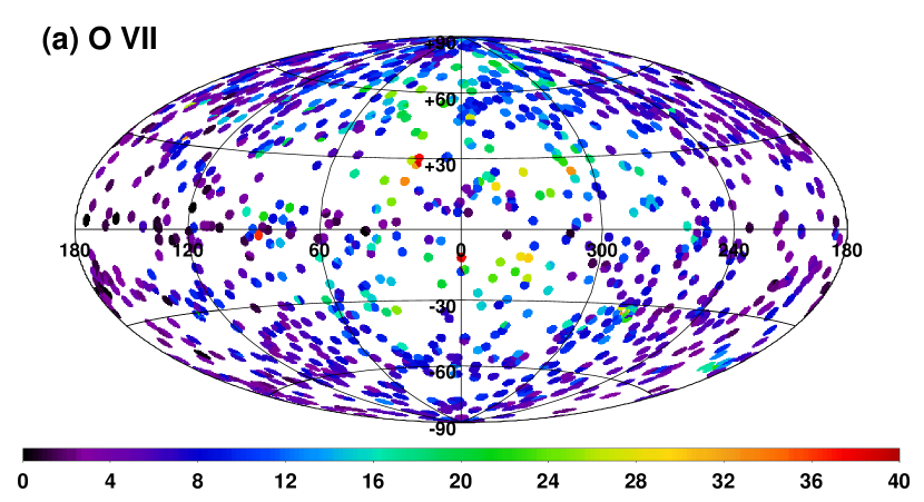
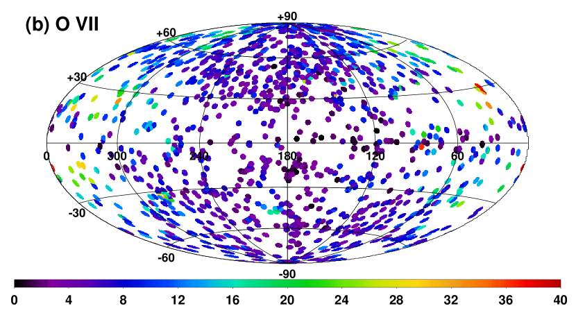
Figure 2.— All-sky maps of the oxygen intensities in L.U., plotted in Galactic coordinates. Panels (a) and (b) show the O VII intensities obtained without the solar wind proton flux filtering described in Section 2.4, in Hammer-Aitoff projections centered on the Galactic Center and the Galactic Anticenter, respectively. Panels (c) and (d) show the O VIII intensities obtained without proton flux filtering in the same projections. Panels (e) through (h) show the corresponding intensities obtained with proton flux filtering. Each intensity measurement is plotted as a colored circle of radius 2° centered on the XMM-Newton pointing direction. If a point on the sky is within 2° of more than one XMM-Newton observation, it is colored according to the nearest observation.

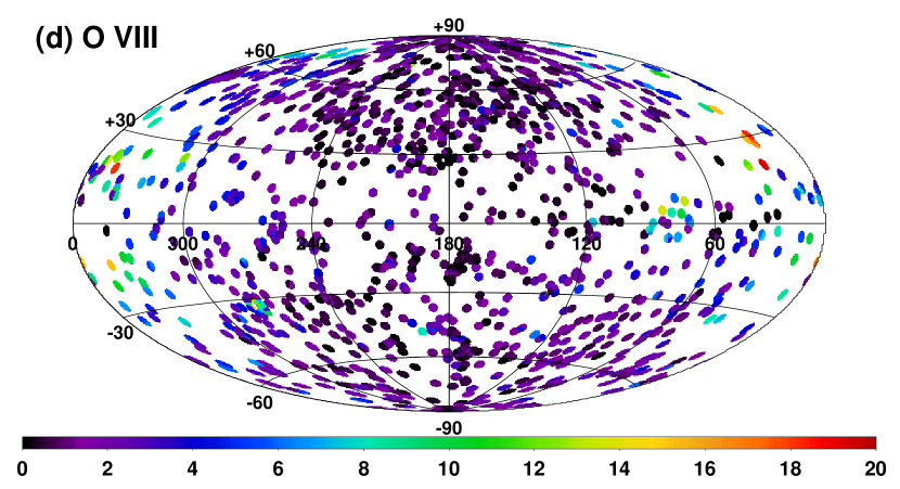
Figure 2.— Continued

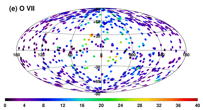
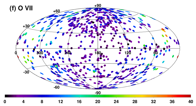
Figure 2.— Continued

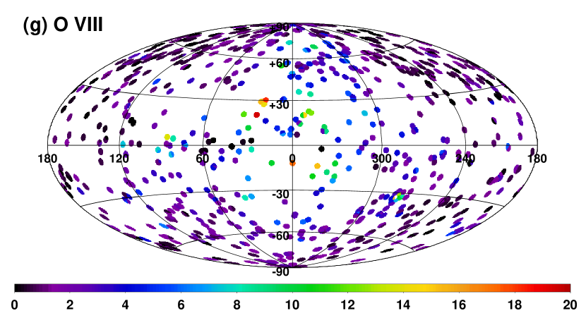
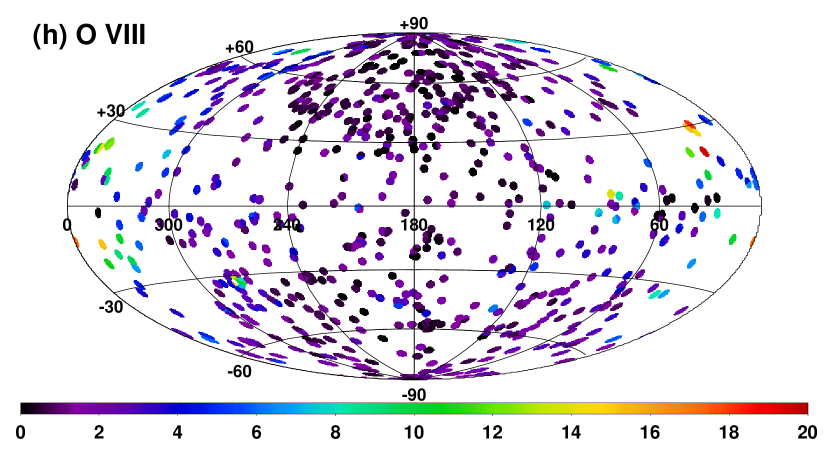
Figure 2.— Continued

Figure 2 shows all-sky maps of the O VII and O VIII intensities, both without (panels (a) through (d)) and with (panels (e) through (h)) proton flux filtering. For each line, we show projections centered on the Galactic Center and on the Galactic Anticenter. Each colored circle in the maps represents an SXRB line intensity measurement. Note that these circles are larger than the XMM-Newton field of view ($\mathrm{radius}=14\arcmin$). See Section 3.8 for a discussion of the sky coverage of our survey. We will discuss the variation in the lines’ intensities over the sky in more detail in Section 4.3, but we note here that the diffuse oxygen emission tends to be brighter toward the Galactic Center ($l<90\arcdeg$ or $l>270\arcdeg$) than toward the Galactic Anticenter.

Figure 6 shows histograms of the O VII and O VIII intensities, both without (solid black lines) and with (gray area) the proton flux filtering. Table 3 contains the ranges and quartiles of the intensities. The quartiles (including the medians) of the oxygen intensities are generally significantly higher than those in Paper I (see Table 3 of that paper). This is because this paper includes the region around the Galactic Center, where the intensities are generally higher (see Figure 2). The quartiles of the O VII intensities obtained without the proton flux filtering are systematically higher than the corresponding quartiles obtained with the proton flux filtering. For O VIII, there are no significant differences in the intensity quartiles with and without the proton flux filtering. We will discuss the effects of proton flux filtering in more detail in Section 3.7.

Figure 6.— Histograms of the (a) O VII and (b) O VIII intensities. The solid black lines show the histograms of intensities obtained without the solar wind proton flux filtering described in Section 2.4, and the gray areas show the histograms of intensities obtained with this filtering.

Table 3Ranges and Quartiles of the Oxygen Intensities

Line	Proton flux	Range	Lower quartile	Median	Upper quartile
	filtering?	(L.U.)	(L.U.)	(L.U.)	(L.U.)
O VII	N	0.00–50.76	3.92 (3.78,4.15)	6.00 (5.90,6.14)	8.74 (8.54,8.97)
O VII	Y	0.00–48.81	3.61 (3.48,3.74)	5.60 (5.36,5.80)	7.95 (7.64,8.29)
O VIII	N	0.00–36.24	0.62 (0.59,0.66)	1.30 (1.24,1.36)	2.36 (2.28,2.45)
O VIII	Y	0.00–24.45	0.56 (0.52,0.61)	1.24 (1.17,1.32)	2.29 (2.19,2.39)

Note. — The numbers in parentheses are the 90% confidence intervals, calculated by bootstrapping.

We will conclude this subsection by looking at the oxygen intensities from the 103 observations identified as being contaminated by geocoronal SWCX emission by Carter et al. (2011, Table A.1). Of these observations, 61 are in our final sample. Of the other 42, 20 were rejected at an early stage of the processing for a variety of reasons (e.g., the target source being too bright), and 22 failed the $F_{\mathrm{total}}^{2-5}/F_{\mathrm{exgal}}^{2-5}\leq 2.7$ requirement. For the remaining 61 observations, the median O VII and O VIII intensities (obtained without proton flux filtering) are 9.83 and 2.19 L.U., respectively, with interquartile ranges of 7.60–13.63 and 1.07–3.18 L.U., respectively. Comparing these values with the medians and quartiles in Table 3, we see that, unsurprisingly, the SWCX-contaminated observations identified by Carter et al. (2011) yield systematically higher oxygen intensities than our survey as a whole.

3.4. Directions with Multiple Observations

Tables 1 and 2 include many directions that have been observed multiple times with XMM-Newton (within a few arcmin). The times between observations of a given direction may range from $\sim$1 day to several years. Multiple observations in the same direction are useful for constraining models of SWCX, as only the SWCX component of the SXRB is expected to vary on such a small timescale.

As XMM-Newton observations of the same target rarely have identical pointing directions, we searched the 1868 good observations in Table 1 for sets of observations whose pointing directions are within 0.1° of each other (cf. the XMM-Newton field of view is $\approx$0.5° across). We found 217 such sets.

Table 4Oxygen Line Intensities from Directions with Multiple Observations

			Paper I			Without proton flux filtering			With proton flux filtering
Dataset	$N_{\mathrm{obs}}$	Obs. ID	Dataset	$l$	$b$	$I_{\mathrm{O\,VII}}$	$I_{\mathrm{O\,VIII}}$		$I_{\mathrm{O\,VII}}$	$I_{\mathrm{O\,VIII}}$
				(deg)	(deg)	(L.U.)	(L.U.)		(L.U.)	(L.U.)
(1)	(2)	(3)	(4)	(5)	(6)	(7)	(8)		(9)	(10)
1	2	0050940401	$\cdots$	0.015	$-12.011$	$35.17^{+1.55}_{-2.29}\pm 2.52$	$15.68^{+1.16}_{-1.35}\pm 6.78$		$35.17^{+1.55}_{-2.29}\pm 2.52$	$15.68^{+1.16}_{-1.35}\pm 6.78$
		0203040401	$\cdots$	359.985	$-11.990$	$33.54\pm 1.79\pm 0.53$	$13.35\pm 1.08\pm 5.71$		$\cdots$	$\cdots$
2	2	0018741701	$\cdots$	3.967	$-59.448$	$11.29\pm 2.03\pm 1.31$	$5.49\pm 1.23\pm 0.55$		$\cdots$	$\cdots$
		0404910801	$\cdots$	3.966	$-59.441$	$6.27^{+1.87}_{-0.91}\pm 1.22$	$0.70^{+0.88}_{-0.57}\pm 1.09$		$\cdots$	$\cdots$
3	2	0057560301	$\cdots$	5.457	$+56.766$	$13.99\pm 0.63\pm 1.11$	$4.71\pm 0.39\pm 2.67$		$13.69^{+0.72}_{-0.76}\pm 0.28$	$5.07\pm 0.46\pm 2.36$
		0148520101	$\cdots$	5.456	$+56.770$	$12.42^{+0.78}_{-0.82}\pm 1.51$	$4.47^{+0.47}_{-0.55}\pm 2.52$		$12.42^{+0.78}_{-0.82}\pm 1.51$	$4.47^{+0.47}_{-0.55}\pm 2.52$
4	2	0400460301	$\cdots$	6.230	$-38.240$	$6.14^{+1.08}_{-0.92}\pm 0.72$	$2.76^{+0.72}_{-0.57}\pm 0.34$		$7.39^{+1.39}_{-1.36}\pm 0.82$	$2.14^{+0.83}_{-0.82}\pm 0.66$
		0400460401	$\cdots$	6.229	$-38.240$	$6.29^{+1.48}_{-1.53}\pm 0.50$	$1.70^{+0.74}_{-0.73}\pm 0.38$		$6.29^{+1.48}_{-1.53}\pm 0.50$	$1.70^{+0.74}_{-0.73}\pm 0.38$
5	3	0401660101	$\cdots$	6.604	$+7.775$	$7.03^{+1.16}_{-0.78}\pm 0.80$	$4.21^{+0.61}_{-0.44}\pm 0.72$		$\cdots$	$\cdots$
		0085582001	$\cdots$	6.588	$+7.785$	$3.84^{+1.64}_{-1.28}\pm 1.78$	$6.01^{+1.28}_{-1.18}\pm 1.17$		$3.84^{+1.64}_{-1.28}\pm 1.78$	$6.01^{+1.28}_{-1.18}\pm 1.17$
		0085581401	$\cdots$	6.588	$+7.786$	$5.15^{+0.82}_{-1.55}\pm 0.99$	$3.97^{+0.99}_{-0.95}\pm 0.97$		$5.15^{+0.82}_{-1.55}\pm 0.99$	$3.97^{+0.99}_{-0.95}\pm 0.97$

Note. — This table is available in its entirety in a machine-readable form in the online journal. A portion is shown here for guidance regarding its form and content.

Table 4 contain the oxygen intensity measurements for directions that have been observed multiple times with XMM-Newton. The sets of observations are ordered by Galactic longitude, $l$. Each set of observations is identified by a unique number (1–217), which is in Column 1, while Column 2 contains the number of observations in each set. Column 3 contains the XMM-Newton observation IDs. Column 4 contains the data set number from Paper I that each observation belonged to, if appropriate (these data sets were numbered from 1 through 69; see Table 5 in Paper I). Note that data set 49 from Paper I is not included in Table 4, because one of the two members of this data set (obs. 0203362201) no longer passes the $F_{\mathrm{total}}^{2-5}/F_{\mathrm{exgal}}^{2-5}$ test, and so is not included in this paper (see Section 3.5, below). Columns 5 and 6 contain the pointing direction in Galactic coordinates. Columns 7 and 8 contain the O VII and O VIII intensities, respectively, measured without the solar wind proton flux filtering described in Section 2.4. As in Tables 1 and 2, the statistical and systematic errors are shown separately. Columns 9 and 10 contain the corresponding measurements obtained with solar wind proton flux filtering. If this filtering rendered an observation unusable, these fields are left blank.

For each of the 217 directions in Table 4, we can place upper limits on the cosmic O VII and O VIII X-ray emission (i.e., the emission that arises beyond the solar system, rather than the emission that is due to SWCX). These upper limits are $\min(I_{\mathrm{O\,VII}})$ and $\min(I_{\mathrm{O\,VIII}})$, which are defined as the minimum O VII and O VIII intensities, respectively, measured in a given direction. These quantities are upper limits on the cosmic oxygen intensities because SWCX may also have contributed photons to the $\min(I)$ measurements. See the top row of Figure 7 for histograms of $\min(I)$. Then, with $\min(I)$ thus defined, $I-\min(I)$ places a lower limit on the SWCX line intensity for a given observation (again, it is a lower limit because SWCX may have contributed photons to the $\min(I)$ measurement).

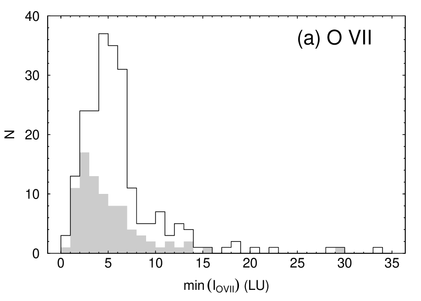
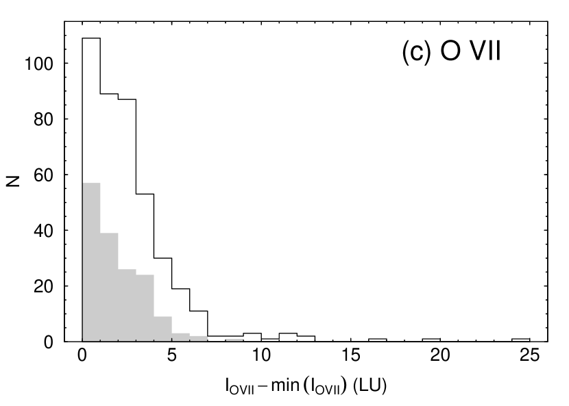
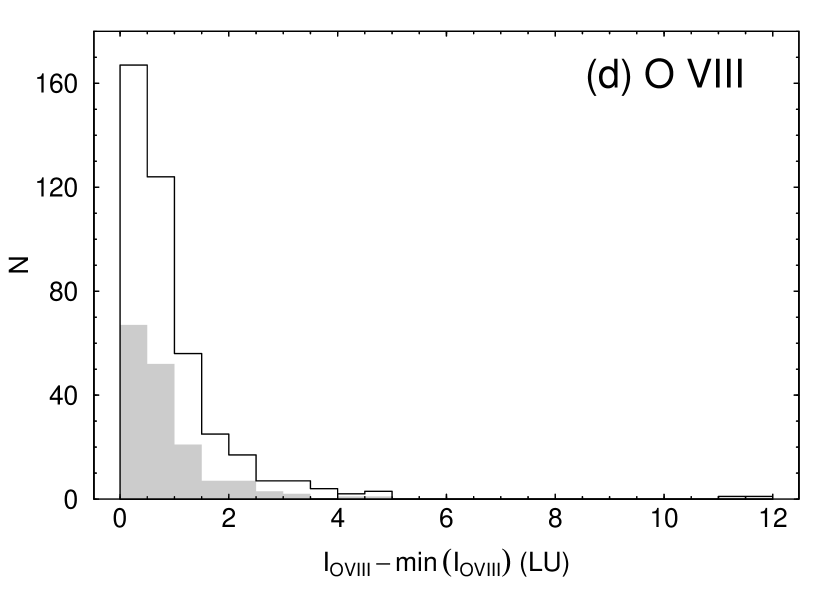
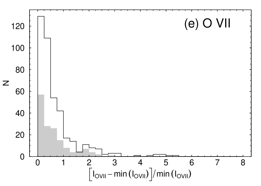
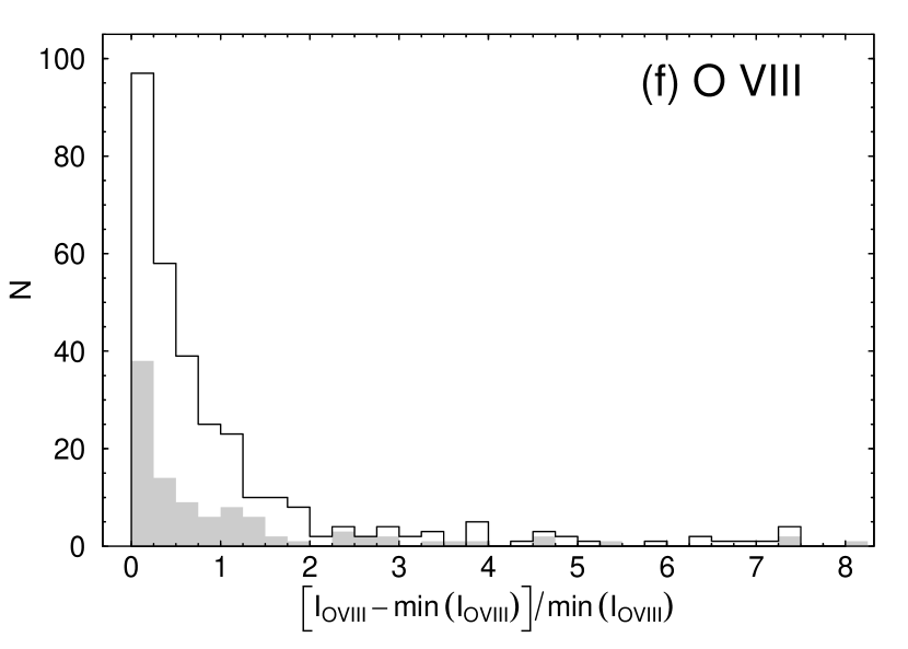
Figure 7.— Top row: Histograms of $\min(I)$ for (a) O VII and (b) O VIII, where $\min(I)$ is the minimum measured intensity in a given direction, and hence the upper limit on the intensity originating in the ISM. Middle row: Histograms of $I-\min(I)$ for (c) O VII and (d) O VIII; here, $\min(I)$ is the minimum measured intensity in the same direction as the $I$ measurement, and hence $I-\min(I)$ is the lower limit on the SWCX X-ray intensity. Bottom row: Histograms of $[I-\min(I)]/\min(I)$ for (e) O VII and (f) O VIII. These histograms were constructed from the data in Table 4. The solid black lines show the results obtained without the solar wind proton flux filtering described in Section 2.4, and the gray areas show the results obtained with this filtering. For each of the 217 sets of observations in Table 4 there is, by definition, an observation with $I-\min(I)=0$; these observations are omitted from Panels (c)–(f). In Panel (e), three observations for which the corresponding values of $\min(I_{\mathrm{O\,VII}})$ are 0 are omitted from both histograms. In Panel (f), nine observations with $[I_{\mathrm{O\,VIII}}-\min(I_{\mathrm{O\,VIII}})]/\min(I_{\mathrm{O\,VIII}})>8$ are omitted from both histograms, while 90 (49) observations for which the corresponding values of $\min(I_{\mathrm{O\,VIII}})$ are 0 are omitted from the histogram showing the results obtained without (with) proton flux filtering.

To show the magnitude of the variability in the oxygen SWCX emission, in the middle row of Figure 7 we plot histograms of $I_{\mathrm{O\,VII}}-\min(I_{\mathrm{O\,VII}})$ and $I_{\mathrm{O\,VIII}}-\min(I_{\mathrm{O\,VIII}})$, obtained with and without the solar wind proton flux filtering described in Section 2.4. For each set of observations, the observation with $I-\min(I)=0$ has been omitted. Similarly to what we found in Paper I, the measured intensity enhancements are typically $\lesssim$5 L.U. for O VII (cf. $\lesssim$4 L.U. stated in Paper I), and $\lesssim$2 L.U. for O VIII (same as stated in Paper I). More quantitatively, the 90th percentile of $I_{\mathrm{O\,VII}}-\min(I_{\mathrm{O\,VII}})$ (excluding the faintest observation from each set) is 5.2 L.U. without proton flux filtering and 3.9 L.U. with. For $I_{\mathrm{O\,VIII}}-\min(I_{\mathrm{O\,VIII}})$, the 90th percentile of $I_{\mathrm{O\,VIII}}-\min(I_{\mathrm{O\,VIII}})$ is 2.0 L.U. without proton flux filtering and 1.9 L.U. with.

The measured O VII enhancements are generally smaller than the corresponding unenhanced intensity, i.e., $I_{\mathrm{O\,VII}}-\min(I_{\mathrm{O\,VII}})$ is typically smaller than $\min(I_{\mathrm{O\,VII}})$; see Figure 7(e) (note that, although we use the term “unenhanced” intensity, $\min(I)$ may still include some photons due to SWCX). The median value of $[I_{\mathrm{O\,VII}}-\min(I_{\mathrm{O\,VII}})]/\min(I_{\mathrm{O\,VII}})$ is 0.39 (0.45) without (with) proton flux filtering, and only 19% (22%) of observations have $[I_{\mathrm{O\,VII}}-\min(I_{\mathrm{O\,VII}})]/\min(I_{\mathrm{O\,VII}})>1$ (the observations that yield the $\min(I_{\mathrm{O\,VII}})$ measurement have been omitted from these values). In contrast, for O VIII, the intensity enhancements are often somewhat brighter than the typical unenhanced intensity; see Figure 7(f). The median value of $[I_{\mathrm{O\,VIII}}-\min(I_{\mathrm{O\,VIII}})]/\min(I_{\mathrm{O\,VIII}})$ is 0.82 (1.39) without (with) proton flux filtering, and 46% (57%) of observations have $[I_{\mathrm{O\,VIII}}-\min(I_{\mathrm{O\,VIII}})]/\min(I_{\mathrm{O\,VIII}})>1$. These results imply that O VIII is typically brighter relative to O VII in the SWCX enhancements than in the baseline SXRB emission.

Some of the observations in Table 4 exhibit particularly bright oxygen intensity enhancements due to SWCX. Nine observations have $I_{\mathrm{O\,VII}}-\min(I_{\mathrm{O\,VII}})>10~{}\mbox{L.U.}$; for three of these observations, the enhancement exceeds 15 L.U.. There are two observations with $I_{\mathrm{O\,VIII}}-\min(I_{\mathrm{O\,VIII}})>5~{}\mbox{L.U.}$ (in fact, these enhancements both exceed 10 L.U.). The observations with $I_{\mathrm{O\,VII}}-\min(I_{\mathrm{O\,VII}})>10~{}\mbox{L.U.}$ or $I_{\mathrm{O\,VIII}}-\min(I_{\mathrm{O\,VIII}})>5~{}\mbox{L.U.}$ are presented in Table 5, along with the observations that yielded the $\min(I)$ in each case. Three of the bright SWCX enhancements in Table 4 were also reported in Paper I. The enhancements measured in Paper I are also shown in the table – the new measurements are consistent with the Paper I measurements. Note that in Paper I we also reported an O VIII enhancement of $\approx$8 L.U. in obs. 0203362201 relative to obs. 0302352201. This enhancement is not included in Table 4 because, as noted above, obs. 0203362201 is not included in this paper (see also Section 3.5, below).

Table 5Directions with the Brightest SWCX Emission

Dataset	Line	Faintest			Brightest		Difference	Paper I
		Obs. ID	$I$		Obs. ID	$I$		Difference
			(L.U.)			(L.U.)	(L.U.)	(L.U.)
12	O VII	0402080801	$5.25^{+1.88}_{-1.48}$		0096010101	$15.28^{+0.97}_{-0.97}$	$10.03^{+1.77}_{-2.12}$	$\cdots$
34	O VII	0206860101	$6.76^{+0.99}_{-1.01}$		0206860201	$19.55^{+2.27}_{-1.54}$	$12.79^{+2.48}_{-1.83}$	$\cdots$
38	O VII	0550061301	$6.45^{+1.89}_{-1.39}$		0041741101	$23.07^{+4.80}_{-4.79}$	$16.62^{+5.00}_{-5.15}$	$\cdots$
40	O VII	0406421401	$5.54^{+1.48}_{-0.85}$		0406420401	$17.14^{+1.71}_{-1.62}$	$11.60^{+1.91}_{-2.20}$	$\cdots$
42	O VII	0400360301	$4.85^{+1.82}_{-1.71}$		0400360801	$17.08^{+1.52}_{-1.45}$	$12.23^{+2.29}_{-2.32}$	$\cdots$
58	O VII	0305920301	$5.80^{+1.42}_{-1.41}$		0305920601	$16.83^{+1.70}_{-1.73}$	$11.03^{+2.21}_{-2.24}$	$\cdots$
83	O VII	0400560301	$3.83^{+0.84}_{-0.63}$		0059140901	$15.45^{+1.42}_{-1.48}$	$11.62^{+1.56}_{-1.70}$	$10.72^{+0.99}_{-0.96}$
90	O VII	0112520901	$4.95^{+1.58}_{-1.71}$		0112520601	$29.28^{+1.83}_{-2.03}$	$24.33^{+2.50}_{-2.57}$	$26.15^{+1.52}_{-1.41}$
107	O VII	0143150301	$3.89^{+1.25}_{-1.61}$		0143150601	$23.26^{+1.25}_{-1.38}$	$19.37^{+2.04}_{-1.86}$	$18.21^{+0.99}_{-1.13}$
38	O VIII	0041740301	$3.62^{+1.87}_{-1.81}$		0041741101	$15.28^{+1.81}_{-1.80}$	$11.66^{+2.56}_{-2.59}$	$\cdots$
138	O VIII	0206090101	$0.02^{+0.88}_{-0.79}$		0206090201	$11.48^{+1.71}_{-1.70}$	$11.46^{+1.89}_{-1.91}$	$\cdots$

As noted in Paper I, the bright O VII enhancements in Table 4 (i.e., those at the bright end of the $I_{\mathrm{O\,VII}}-\min(I_{\mathrm{O\,VII}})$ distribution) are of interest because they are much larger than most measurements of O VII SWCX enhancements ($\lesssim$7 L.U.; Snowden et al. 2004; Fujimoto et al. 2007; Henley & Shelton 2008; Gupta et al. 2009; see also Figure 7(c)). However, since Paper I, bright O VII enhancements of 14–21 and 36 L.U. have also been reported by Carter et al. (2011) and Ezoe et al. (2011), respectively. Note that these enhancements were found by looking at line intensity variations within XMM-Newton or Suzaku observations, rather than between observations, as we have done. Note also that Koutroumpa et al. (2007) reported O VII enhancements of up to 10 L.U., but we found the observations in question to be badly contaminated by soft protons (see Paper I).

Similarly to the brightest O VII enhancements, the brightest O VIII enhancements (reported in Table 4) are much larger than those that are typically measured ($\lesssim$2 L.U.; Henley & Shelton 2008; Gupta et al. 2009; see also Figure 7(d)), although O VIII enhancements of 6.5 and 5.0 L.U. were reported by Snowden et al. (2004) and Fujimoto et al. (2007), respectively. More recently, O VIII enhancements of 26 and 12 L.U. have been reported by Carter et al. (2010) and Ezoe et al. (2011), respectively, in both cases associated with coronal mass ejections.

3.5. Differences from Paper I

The main differences in our current methodology from that in Paper I are summarized as follows:

1. We used a more recent version of the SAS software (11.0.1 versus 7.0.0), which incorporates the XMM-ESAS software (Section 2). The version of mos_back included in SAS version 11.0.1 can automatically detect anomalous CCDs. For some of the observations that were in Paper I, mos_back detected anomalous CCDs that we had failed to identify in Paper I (Section 2.5).

2. For the automated source removal, we used data from the XMM-Newton Serendipitous Source Catalogue, instead of carrying out source detection ourselves on each observation. We also used larger circles to exclude such sources (50″ versus $\approx$30″–40″; Section 2.3).

3. In the spectral analysis, we used an unbroken power-law to model the residual soft-proton contamination, as opposed to a broken power-law in Paper I. Unlike Paper I, we placed constraints on this power-law’s spectral index (Section 3.1).

4. We used a lower normalization for the EPL in our spectral model (7.9 versus 10.5 photons $\mbox{cm}^{-2}$ $\mbox{s}^{-1}$ $\mbox{sr}^{-1}$ $\mbox{keV}^{-1}$; Section 3.1). In addition, we estimated the size of systematic errors associated with our assuming this normalization, and with our assuming that the non-oxygen line emission can be modeled with an APEC model (Section 3.2).

5. We used $\chi^{2}_{\mathrm{min}}+2.30$ (Lampton et al., 1976; Avni, 1976) to calculate the statistical errors on the oxygen intensities (although not explicitly stated, we used $\chi^{2}_{\mathrm{min}}+1.0$ in Paper I, which is only valid for the error on a single interesting parameter; Lampton et al. 1976). These larger statistical errors, combined with the systematic errors mentioned above, result in confidence intervals that are typically $\sim$2 times wider than those in Paper I.

Because of the improvement in anomalous-CCD detection and the changes in the automated source removal, there are some differences in the solid angles from which the SXRB spectra were extracted (columns 6 and 8 in Tables 1 and 2). In addition, because of differences between the OMNIWeb data used in this paper (downloaded on 2011 March 01) and that used in Paper I (downloaded on 2009 February 12), there are, in a few cases, significant differences in the amount of good time that remains after the proton flux filtering has been applied (columns 5 and 7 in Table 2). For example, in obs. 0205590301, the post-filtering good time has decreased from $\approx$41 ks per camera in Paper I to $\approx$9 ks. This is because the observed solar wind proton flux was close to the threshold of $2\times 10^{8}$ $\mbox{cm}^{-2}$ $\mbox{s}^{-1}$ during this observation. In the OMNIWeb data used in Paper I, the observed solar wind proton flux was generally below this threshold, whereas in the revised proton flux data used in this paper, the observed flux was generally above this threshold. Finally, note that for obs. 0203900101 we used two exposures per camera in Paper I. However, upon reinspecting this observation, we have concluded that the two shorter exposures are likely contaminated by soft protons. We have therefore rejected these two exposures, and just use the longer exposures (one per camera) in this paper.

Despite these differences, the new oxygen intensity measurements are generally not significantly different from those in Paper I. Here, we discuss the few observations for which this is not the case.

Table 6Observations from Paper I that are Missing from the Current Paper

Obs. ID	Reason
Without Proton Flux Filtering
0010620101	$F_{\mathrm{total}}^{2-5}/F_{\mathrm{exgal}}^{2-5}>2.7$
0065820101	$F_{\mathrm{total}}^{2-5}/F_{\mathrm{exgal}}^{2-5}>2.7$
0099030101	$F_{\mathrm{total}}^{2-5}/F_{\mathrm{exgal}}^{2-5}>2.7$
0109270701	$F_{\mathrm{total}}^{2-5}/F_{\mathrm{exgal}}^{2-5}>2.7$
0111490401	Diffraction spikes
0128531501	$F_{\mathrm{total}}^{2-5}/F_{\mathrm{exgal}}^{2-5}>2.7$
0134540101	Diffraction spikes
0201951701	Insufficient good time
0203362201	$F_{\mathrm{total}}^{2-5}/F_{\mathrm{exgal}}^{2-5}>2.7$
0203610201	$F_{\mathrm{total}}^{2-5}/F_{\mathrm{exgal}}^{2-5}>2.7$
0206060201	$F_{\mathrm{total}}^{2-5}/F_{\mathrm{exgal}}^{2-5}>2.7$
0206360101	$F_{\mathrm{total}}^{2-5}/F_{\mathrm{exgal}}^{2-5}>2.7$
0302260201	$F_{\mathrm{total}}^{2-5}/F_{\mathrm{exgal}}^{2-5}>2.7$
0305290201	$F_{\mathrm{total}}^{2-5}/F_{\mathrm{exgal}}^{2-5}>2.7$
0405730401	$F_{\mathrm{total}}^{2-5}/F_{\mathrm{exgal}}^{2-5}>2.7$
0411980601	$F_{\mathrm{total}}^{2-5}/F_{\mathrm{exgal}}^{2-5}>2.7$
With Proton Flux Filtering
0083000101	$F_{\mathrm{total}}^{2-5}/F_{\mathrm{exgal}}^{2-5}>2.7$
0099030101	$F_{\mathrm{total}}^{2-5}/F_{\mathrm{exgal}}^{2-5}>2.7$
0109270701	$F_{\mathrm{total}}^{2-5}/F_{\mathrm{exgal}}^{2-5}>2.7$
0110950201	Insufficient good time
0111100101	$F_{\mathrm{total}}^{2-5}/F_{\mathrm{exgal}}^{2-5}>2.7$
0134540101	Diffraction spikes
0141980601	Insufficient good time
0141980701	Insufficient good time
0148560501	Insufficient good time
0150320201	$F_{\mathrm{total}}^{2-5}/F_{\mathrm{exgal}}^{2-5}>2.7$
0158560301	Insufficient good time
0162160401	Insufficient good time
0200430401	Insufficient good time
0200810301	Insufficient good time
0201040101	Insufficient good time
0201940201	Insufficient good time
0203360701	Insufficient good time
0203361701	Insufficient good time
0203610201	$F_{\mathrm{total}}^{2-5}/F_{\mathrm{exgal}}^{2-5}>2.7$
0203840101	Insufficient good time
0206360101	$F_{\mathrm{total}}^{2-5}/F_{\mathrm{exgal}}^{2-5}>2.7$
0305290201	$F_{\mathrm{total}}^{2-5}/F_{\mathrm{exgal}}^{2-5}>2.7$

The current catalog excludes 16 (22) observations that were included in the Paper I results obtained without (with) proton flux filtering. These observations are shown in Table 6, along with the reason for their exclusion. The most common reasons for exclusion are either that the observation now exceeds our $F_{\mathrm{total}}^{2-5}/F_{\mathrm{exgal}}^{2-5}$ threshold for excluding soft-proton-contaminated observations (see Section 3.3), or that the observation no longer has sufficient good time after being reprocessed (see Sections 2.1 and 2.4). In two cases (obs. 0111490401 and 0134540101), we found upon reinspection that there are diffraction spikes from the target sources (VY Ari and HR 1099, respectively) visible in the soft band (0.2–0.9 keV) images. As photons in these diffraction spikes would contaminate our SXRB measurements, we decided to err on the side of caution and reject these observations.

Table 7Observations with Oxygen Intensities Significantly Different from Those in Paper I

	$I_{\mathrm{O\,VII}}$
	(L.U.)
Obs. ID	Paper I	This paper
0108062101	$5.96^{+0.19}_{-0.43}$	$4.61^{+0.49}_{-0.48}$
0147511801	$8.04^{+0.41}_{-0.23}$	$6.58\pm 0.60$
0301600101	$3.69^{+0.42}_{-0.20}$	$2.39^{+0.52}_{-0.51}$

There are only three observations for which either the O VII or O VIII intensity measurements differs by more than $2\sigma$ from the Paper I value. In all three cases, it is the O VII intensity measured without proton flux filtering that is different: the intensities measured in this paper are lower than the Paper I values (see Table 7).

For obs. 0147511801 and 0301600101, the difference in O VII intensity from Paper I seems to be mainly due to our using a smaller normalization for the EPL in this paper. Having a smaller normalization for the EPL results in a larger normalization for the soft-proton model. These two model components have different spectra: the soft-proton model increases monotonically with decreasing energy, while the EPL, being subject to Galactic absorption and the response of the X-ray telescope, decreases with decreasing energy below $\sim$1 keV. As a result, the net effect of decreasing the normalization of the EPL (and thus increasing that of the soft-proton model) is to increase the combined number of counts from these two components in the vicinity of the oxygen lines. This in turn leads to a decrease in the number of counts attributed to the oxygen lines, and hence a decrease in the oxygen intensity. While this effect should, in principle, affect all observations, clearly in the vast majority of cases the effect is negligible compared with the combined statistical and systematic error.

For obs. 0108062101, the above explanation may partly explain the difference in O VII intensity. In addition, the new version of mos_back identified the MOS1.5 chip as being anomalous in this observation, whereas we failed to identify it as such in Paper I. Including an anomalous chip for this observation in Paper I may have led to an inaccurate estimate of the particle background, and hence to an inaccurate measurement of the O VII intensity.

3.6. Contamination from Bright Sources and Soft Protons

In Paper I we examined the possibilities that contamination from the wings of the PSF of bright sources and/or contamination from soft protons were biasing our intensity measurements. We came to the conclusion that neither was a significant source of bias. Using the same methods as in Paper I, we come to the same conclusion here.

To examine possible contamination from bright sources, we considered the observations in our sample for which we had excised the target source by hand ($\sim$30% of our sample). For each observation, we incrementally increased the source exclusion radius (typically in five 1′ increments), and remeasured the oxygen intensities each time. If photons in the wings of the PSF were biasing our measurements, we would expect the measured intensity to decrease with increasing source exclusion radius. For each observation, we used $\chi^{2}$ to test whether the intensities measured with larger source exclusion radii were consistent with the original intensity measurement.

We found that for $\approx$6% of the observations, the O VII and/or O VIII intensities measured with larger source exclusion radii were not consistent with the original measurements at the 5% level. However, upon inspecting the intensities as a function of source exclusion radius, we found that in most cases the variation was non-monotonic, or that the intensities increased with source exclusion radius. Neither of these forms of variation is consistent with there being contamination from the target source. For only five observations were there indications of contamination from the target source. For these observations, we simply increased the source exclusion radius to the point where the intensities stopped varying with source exclusion radius (an increase of 1′ or 2′). Having corrected these five observations, we think that our intensity measurements are not seriously contaminated by emission from bright sources.

We also investigated the possibility of contamination from fainter sources, i.e., the sources removed by the automated source removal (Section 2.3) rather than by hand. We reprocessed 100 of our observations, chosen at random, with the source exclusion radius used in the automated source removal increased by 50% from 50″ to 75″. The intensities obtained using this larger source exclusion radius were not significantly different from our original measurements, nor was there any systematic shift in the intensities toward larger or smaller values. We therefore conclude that our intensity measurements are not seriously contaminated by emission from fainter, automatically removed sources.

To examine the possibility that soft-proton contamination is biasing our results, we looked for any correlation between $I-\min(I)$ and $F_{\mathrm{total}}^{2-5}/F_{\mathrm{exgal}}^{2-5}$ (the latter being a measure of the amount of soft-proton contamination). For a given direction, any variation in intensity should be solely due to SWCX, and so, in the absence of any bias, there should be no correlation between $I-\min(I)$ and $F_{\mathrm{total}}^{2-5}/F_{\mathrm{exgal}}^{2-5}$. For O VII and O VIII, the correlation coefficients (specifically, Kendall’s $\tau$; e.g., Press et al. 1992) are $-0.08$ $(-0.13,-0.04)$ and $-0.02$ $(-0.07,+0.03)$, respectively (the values in parentheses are the 90% bootstrap confidence intervals). Although the correlation coefficient for $I_{\mathrm{O\,VII}}-\min(I_{\mathrm{O\,VII}})$ against $F_{\mathrm{total}}^{2-5}/F_{\mathrm{exgal}}^{2-5}$ is different from zero at a statistically significant level, it is still small in magnitude ($|\tau|\leq 0.1$). When we use other measures of the soft-proton contamination (the normalization of the power-law model, or its spectral index), we again find correlation coefficients that are small in magnitude ($|\tau|\leq 0.1$), and that are typically consistent with zero. Hence, soft-proton contamination is unlikely to be seriously biasing our intensity measurements.

3.7. Effect of Proton Flux Filtering

Here we discuss the effects of excluding the portions of the XMM-Newton data taken when the solar wind proton flux exceeded $2\times 10^{8}$ $\mbox{cm}^{-2}$ $\mbox{s}^{-1}$. This filtering was carried out in an attempt to reduce the contamination due to SWCX emission, and is described in Section 2.4. As noted in Section 3.3, the quartiles of the O VII intensities obtained without this filtering are systematically higher than the corresponding quartiles obtained with the filtering, while for O VIII, there are no significant differences in the intensity quartiles with and without the proton flux filtering. However, this does not mean that the proton flux filtering leads to systematically lower O VII intensities being extracted from the SXRB spectra. When we look at the 356 observations for which proton flux filtering had some effect, but did not render the observation unusable (denoted by a “Y” in Column 14 of Table 2), we find that the median difference in the O VII intensity without and with proton flux filtering is $-0.02~{}\mbox{L.U.}$ (90% bootstrap confidence interval: $-0.10$ to 0.03 L.U.). For O VIII the corresponding difference is 0.00 L.U. ($-0.01$ to 0.03 L.U.). Thus, as we found in Paper I, proton flux filtering does not lead to systematically lower oxygen intensities being extracted from the SXRB spectra.

In contrast, proton flux filtering does preferentially remove the observations that yield the largest O VII intensities (i.e., during such observations the solar wind proton flux tended to exceed $2\times 10^{8}$ $\mbox{cm}^{-2}$ $\mbox{s}^{-1}$). Of the 336 observations in Table 1 with $I_{\mathrm{O\,VII}}>10~{}\mbox{L.U.}$, 135 (40%) yield usable spectra after the proton flux filtering, compared with 856 out of 1532 (56%) of the observations with $I_{\mathrm{O\,VII}}\leq 10~{}\mbox{L.U.}$. For $I_{\mathrm{O\,VII}}>15~{}\mbox{L.U.}$, the fraction is 45 out of 118 observations (38%), compared with 946 out of 1750 (54%) for observations with $I_{\mathrm{O\,VII}}\leq 15~{}\mbox{L.U.}$. This tendency of proton flux filtering to preferentially remove the observations that yield larger O VII intensities explains why there is a significant downward shift in the quartiles of the O VII intensities when proton flux filtering is included (Table 3). However, it should be noted that this tendency is less pronounced than we found in Paper I: in Paper I, only 5 out of 31 observations (16%) with $I_{\mathrm{O\,VII}}>10~{}\mbox{L.U.}$, and 1 out of 9 observations (11%) with $I_{\mathrm{O\,VII}}>15~{}\mbox{L.U.}$ yielded usable spectra after the proton flux filtering. This difference may be due to the fact that the oxygen intensities in the region covered by Paper I ($l=120\arcdeg$–240°) are generally lower than those toward the Galactic Center (see Figure 2), and so a bright O VII line in Paper I was more likely to be due to SWCX, and thus more likely to be associated with a large solar wind proton flux. Despite the fact that a larger fraction of the observations with larger O VII intensities was rejected by the proton flux filtering, in Paper I we did not see a significant downward shift in the O VII intensity quartiles when proton flux filtering was included. Presumably this is because the observations with the largest O VII intensities were a small subset of the Paper I sample.

For O VIII, observations with large and small intensities yield usable spectra after the proton flux filtering at similar rates: 81 out of 161 observations (50%) with $I_{\mathrm{O\,VIII}}>5~{}\mbox{L.U.}$, compared with 910 out of 1707 observations (53%) with $I_{\mathrm{O\,VIII}}\leq 5~{}\mbox{L.U.}$. In contrast, in Paper I, only 2 out 9 observations (22%) with $I_{\mathrm{O\,VIII}}>5~{}\mbox{L.U.}$ yielded usable spectra after the proton flux filtering. The fact that observations with large and small O VIII intensities yield usable spectra after the proton flux filtering at similar rates explains the similarity of the O VIII intensity quartiles in Table 3 with and without proton flux filtering.

3.8. Survey Sky Coverage

Figure 8.— All-sky maps in Galactic coordinates showing how our oxygen intensity measurements are distributed on the sky. The large numbers show the number of oxygen intensity measurements in each of 12 equal-area regions of the sky. The small numbers underneath show the percentage of observations in our survey (S), and percentage of the original set of 5698 archival observations (A) that fall within each region (in some cases the percentages do not sum to 100 due to rounding). If the observations were uniformly distributed, each region would have 8.3% of the observations. Panel (a) shows the number intensity measurements obtained without the solar wind proton flux filtering described in Section 2.4, while panel (b) shows the numbers of intensity measurements obtained with this filtering.

In general our measurements are well distributed over the sky, albeit with some large scale variation in the sky coverage (see the maps in Figure 2, and also Figure 8, which gives the number of oxygen intensity measurements in 12 equal-area regions of the sky). There appear to be fewer observations at low Galactic latitudes ($|b|<30\arcdeg$) than at higher latitudes. We see from Figure 8 that low latitudes away from the Galactic Center ($l=60\arcdeg$–300° and $|b|<30\arcdeg$) are relatively undersampled in our final sample, with 23% of the observations lying in this third of the sky. This is largely due to the relatively lower coverage of this region of the sky in the XMM-Newton archive – 25% of the archival observations are toward this third of the sky. Higher latitudes away from the Galactic Center are relatively oversampled in our final sample – 53% of the observations in our final sample are in the third of the sky with $l=60\arcdeg$–300° and $|b|\geq 30\arcdeg$. This is partly because this region of the sky is oversampled in the archive, with 40% of the archival observations lying in this third of the sky. It is not clear why a larger fraction of the observations in this region of the sky make it to our final sample.

There also appear to be fewer observations toward the inner Galaxy ($l<60\arcdeg$ or $l>300\arcdeg$) than away from the inner Galaxy. Higher latitudes toward the inner Galaxy ($l<60\arcdeg$ or $l>300\arcdeg$, $|b|\geq 30\arcdeg$) may appear undersampled in Figure 2 in comparison to the relative oversampling of the adjacent high-latitude regions.

The region immediately around the Galactic Center ($l<60\arcdeg$ or $l>300\arcdeg$, $|b|<30\arcdeg$) is undersampled in our final sample – only 7% of our final set of observations lie in this sixth of the sky, compared with 20% of the archival observations. This is for a number of reasons. First, observations in this region of the sky are rejected at a higher rate by the light curve filtering described in Section 2.1, for reasons that are unclear. Second, observations in this region of the sky are rejected at a higher rate due to the presence of bright point sources, bright diffuse emission, or bright arcs in the field of view (see Section 2.1). Finally, observations in this region of the sky are rejected at a higher rate due to $F_{\mathrm{total}}^{2-5}/F_{\mathrm{exgal}}^{2-5}$ exceeding 2.7 (this threshold was introduced in Section 3.3, and is intended for the identification and rejection of observations with excessive soft-proton contamination). Approximately 3/4 of the observations in this region of the sky that were rejected in this way are toward very low latitudes ($|b|<3\arcdeg$), and thus their SXRB spectra likely exhibit the hard X-ray emission from the Galactic Ridge (e.g., Worrall et al., 1982; Revnivtsev et al., 2006). This additional hard emission would tend to increase $F_{\mathrm{total}}^{2-5}$ relative to $F_{\mathrm{exgal}}^{2-5}$. While such observations are not necessarily badly contaminated by soft protons, we erred on the side of caution and rejected all observations with $F_{\mathrm{total}}^{2-5}/F_{\mathrm{exgal}}^{2-5}>2.7$. Note also that our spectral model (Section 3.1) is designed for the analysis of spectra in which counts above $\sim$2 keV are from either the EPL or from residual soft-proton contamination. Re-analyzing the spectra with a model that is better suited to modeling the Galactic Ridge emission is beyond the scope of this survey.

4. DISCUSSION

4.1. Implications for Solar Wind Charge Exchange

Several factors affect the intensity of the SWCX emission in a given observation of the SXRB. The geocoronal SWCX intensity is expected to depend on the solar wind proton flux near the Earth, and on where the sightline passes through the magnetosheath (e.g., Robertson & Cravens, 2003a, b; Robertson et al., 2006). The heliospheric SWCX intensity is expected to depend on the phase of the solar cycle, the ecliptic latitude, and the location of the Earth in its orbit (e.g., Robertson & Cravens, 2003a; Koutroumpa et al., 2006). Variations in the solar wind ion composition, or the passage of a coronal mass ejection across the line of sight (e.g., Koutroumpa et al., 2007; Henley & Shelton, 2008; Carter et al., 2010) can also affect the SWCX intensity.

A detailed study of all the above factors is beyond the scope of this catalog paper. However, we will point out a few interesting features of our data, and discuss them in the context of simple SWCX models. First, we will consider the heliospheric SWCX emission, and its variation with ecliptic latitude and phase of the solar cycle. Then, in Section 4.1.2, we will consider the geocoronal SWCX emission, and compare the observed variations in intensity with those expected from a simple model of the emission.

4.1.1 Heliospheric SWCX Emission

Model Expectations

To determine how the heliospheric SWCX emission is expected to vary with ecliptic latitude and with phase of the solar cycle, we refer to the heliospheric SWCX model of Koutroumpa et al. (2006). Sightlines toward low ecliptic latitudes sample the slow solar wind (and hence approximately the same density of solar wind O⁺⁷ and O⁺⁸ ions) throughout the solar cycle. During solar minimum, the photoionization of neutral H and He is less efficient, leading to greater densities of these atoms. Hence, the oxygen intensities at low ecliptic latitudes are expected to be higher during solar minimum than at solar maximum (Koutroumpa et al., 2006). In contrast, sightlines toward high ecliptic latitudes only experience the slow solar wind (in which O⁺⁷ and O⁺⁸ are relatively abundant) during solar maximum; they experience the fast solar wind (in which O⁺⁷ and O⁺⁸ are less abundant) during solar minimum. Thus, we expect the X-ray intensities at high ecliptic latitudes to be higher during solar maximum. Furthermore, during solar maximum the intensities are not expected to be strongly dependent on ecliptic latitude, whereas during solar minimum the intensities are expected to be higher at low ecliptic latitudes (see Figures 1 and 11–13 in Koutroumpa et al. 2006).

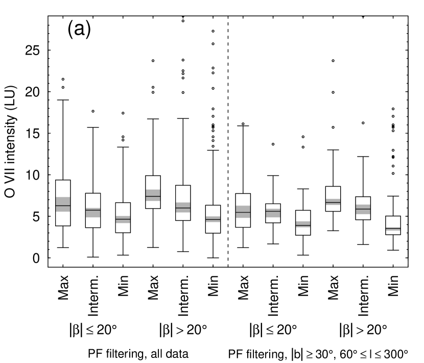
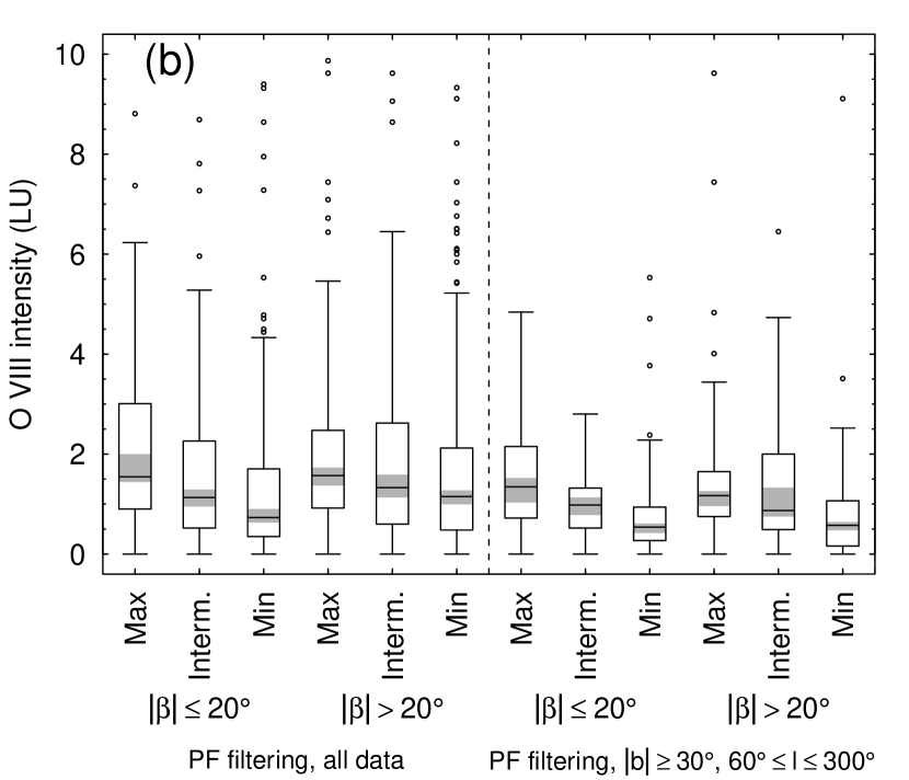
Figure 9.— Boxplots showing the intensity of (a) O VII and (b) O VIII for different ecliptic latitudes ($|\beta|\leq 20\arcdeg$ versus $|\beta|>20\arcdeg$) and for different phases in the solar cycle (see text for details). Each box indicates the median and the lower and upper quartiles, and the whiskers extend to the most extreme data point that is no more than twice the interquartile range from the box. Outliers are plotted individually with open circles. The gray bands indicate the 90% confidence intervals on the medians, calculated by bootstrap resampling. The boxes in the left-hand region of each panel show the results for measurements obtained with the proton flux (PF) filtering described in Section 2.4, with observations identified as SWCX-contaminated by Carter et al. (2011) excluded. The boxes in the right-hand regions show the same data, but with observations toward low Galactic latitudes ($|b|<30\arcdeg$) or toward the inner Galaxy ($l>60\arcdeg$ or $l<300\arcdeg$) excluded.

Comparison with Observations

In order to test these ideas, we present the distributions of the O VII and O VIII intensities (from the proton-flux-filtered measurements, having excluded the observations identified as SWCX-contaminated by Carter et al. 2011). The boxplots presented in Figure 9 are categorized by ecliptic latitude and by phase of the solar cycle. For example, the first box in each panel shows the intensity distribution for observations toward low ecliptic latitudes made during solar maximum (“Max”). Here, we define solar maximum as being before 00:00UT on 2003 Feb 01 ($\mbox{MJD}=52,671$), and solar minimum (“Min”) as being after 00:00UT on 2005 Jun 01 ($\mbox{MJD}=53,522$), with an intermediate phase (“Interm.”) between these times. The left-hand regions of the plots show the results for all of the measurements, while in the right-hand regions we have excluded observations toward low Galactic latitudes or toward the inner Galaxy (to reduce the confounding effects of the variation in intensity with Galactic latitude and longitude; see Section 4.3, below).

Although the distributions of the intensities are rather broad, there is a clear systematic decrease in the intensities from solar maximum to solar minimum. While this is expected at high ecliptic latitudes, it is the opposite of what is expected at low ecliptic latitudes (Koutroumpa et al. 2006; see Model Expectations, above). As we have used the proton-flux-filtered data, the unexpected trend at low ecliptic latitudes is unlikely to be due to systematic differences in the geocoronal SWCX intensity with solar cycle. A possible explanation is that, during solar maximum, observations at all latitudes are more likely to be affected by SWCX emission from a coronal mass ejection moving across the line of sight than during solar minimum.

We searched for systematic differences between the intensities toward high and low ecliptic latitudes, by checking whether or not the confidence intervals on the median intensities overlapped. We considered only the data plotted in right-hand regions of Figures 9(a) and 9(b), to reduce the possibility of the variation with Galactic coordinates affecting the results. The O VII intensities measured during solar minimum tend to be slightly higher toward low ecliptic latitudes. Although the difference is not large, this trend is at least qualitatively as expected (Koutroumpa et al. 2006; see Model Expectations, above). During solar maximum, the O VII intensities tend to be higher toward high ecliptic latitudes, which is not as expected (see Model Expectations, above). In contrast, for the O VIII measurements in the right-hand region of Figure 9(b), the median intensities measured toward high and low ecliptic latitudes are consistent with each other, for all three phases of the solar cycle (maximum, intermediate, and minimum).

4.1.2 Geocoronal SWCX Emission

We now consider the geocoronal SWCX emission. In Paper I we showed that the solar wind proton flux alone is not a good indicator of the degree of SWCX contamination in an SXRB spectrum: for several directions with multiple XMM-Newton observations, we found that the oxygen intensity decreased with increasing proton flux. We also found that there was no clear tendency for sightlines that pass close to or through the sub-solar region of the magnetosheath (that is, the region near the Earth-Sun line) to yield systematically higher oxygen intensities, contrary to expectations (Robertson & Cravens, 2003b).

Our new, larger dataset leads us to the same conclusions. However, rather than re-creating Figures 13 and 15 from Paper I with our new data, here we will look at the geocoronal SWCX in a different way, using a model that is similar to that described in Robertson & Cravens (2003b).

Geocoronal SWCX Model

The geocoronal SWCX intensity is given by

$$I_{\mathrm{geo}}=\frac{1}{4\pi}\int\alpha n_{\mathrm{sw}}\bar{u}n_{\mathrm{H}}dl,$$ (3)

where $\alpha$ is the product of the relevant charge exchange cross-section, line yield, ion fraction, and elemental abundance, $n_{\mathrm{sw}}$ is the solar wind proton density, $\bar{u}$ is the mean ion-neutral collision speed (denoted by $\langle g\rangle$ in Robertson & Cravens 2003b), and $n_{\mathrm{H}}$ is the hydrogen density in the Earth’s exosphere. The integral is carried out along the line of sight. The mean ion-neutral collision speed is given by

$$\bar{u}\approx\left(u_{\mathrm{sw}}^{2}+v_{\mathrm{th}}^{2}\right)^{1/2}=\left(u_{\mathrm{sw}}^{2}+3kT/m\right)^{1/2},$$ (4)

where $u_{\mathrm{sw}}$ is the bulk solar wind speed, and $v_{\mathrm{th}}$ is the thermal speed of an ion of mass $m$ in solar wind gas of temperature $T$.

If we assume that $\alpha$ is approximately constant along each line of sight, and approximately the same for each observation, then the difference in the geocoronal SWCX intensity between two observations of the same direction would be proportional to the difference in $\int n_{\mathrm{sw}}\bar{u}n_{\mathrm{H}}dl$ between the two observations. If we also assume for now that the heliospheric SWCX intensity is approximately constant in a given direction, we would expect

$$I-\min(I)\approx\frac{\alpha}{4\pi}\Delta\left\{\int n_{\mathrm{sw}}\bar{u}n_{\mathrm{H}}dl\right\},$$ (5)

where $\min(I)$ is as defined in Section 3.4, and the $\Delta$ indicates the difference in the integral between the observations that yielded $I$ and $\min(I)$.

For comparison with the observed values of $I-\min(I)$, we estimated the right-hand side of Equation (5) for each observation in Table 4. In particular, we calculated the time-averaged value of $\int n_{\mathrm{sw}}\bar{u}n_{\mathrm{H}}dl$ during each observation, including only the good times from our data processing, and taking into account XMM-Newton’s changing position and the variation in the incident solar wind. For the exospheric hydrogen density, we assumed $n_{\mathrm{H}}(r)=(25~{}\mbox{cm}^{-3})(10R_{\mathrm{E}}/r)^{3}$, where $r$ is the distance from the center of the Earth, and $R_{\mathrm{E}}$ is the radius of the Earth (Cravens et al., 2001). For the solar wind density, speed, and temperature in the magnetosheath, we used the magnetosphere model of Spreiter et al. (1966, Figures 10 and 11), assuming that the distance from the Earth’s center to the magnetopause along the Earth-Sun line is $10R_{\mathrm{E}}$. For the pre-bowshock solar wind density, speed, and temperature, we used data from OMNIWeb. We assumed that changes in the incident solar wind occurred instantaneously across the domain of the Spreiter et al. (1966) model. As the time-resolution of the solar wind data is 1 h, and the solar wind takes $\lesssim 30R_{\mathrm{E}}/(400~{}\mbox{km}\ \mbox{s}^{-1})=8$ min to cross the model domain, this is a reasonable approximation. We calculated $\alpha$ for O VII ($3.8\times 10^{-19}~{}\mbox{cm}^{2}$) and O VIII ($2.2\times 10^{-19}~{}\mbox{cm}^{2}$) using the slow solar wind values from Table 1 of Koutroumpa et al. (2006), assuming a line yield of 1.

Comparison with Observations

Figure 10 shows $I_{\mathrm{O\,VII}}-\min(I_{\mathrm{O\,VII}})$ and $I_{\mathrm{O\,VIII}}-\min(I_{\mathrm{O\,VIII}})$ against $\Delta\left\{\int n_{\mathrm{sw}}\bar{u}n_{\mathrm{H}}dl\right\}$. As we wish to look at the influence of the solar wind on the geocoronal SWCX, we use the results obtained without proton flux filtering, and do not exclude the observations identified as SWCX-contaminated by Carter et al. (2011). To reduce the effect that the variation of the heliospheric SWCX with solar cycle phase has on $I-\min(I)$, and to allow us to concentrate on variations in the geocoronal SWCX, we present various solar cycle phase-based subsets of the data in Figure 10. The top panels show the results for all the observations in Table 4. The other panels show the results for different phases of the solar cycle (as defined earlier). Note that, in the (say) solar maximum panels, $\min(I)$ means the minimum intensity measured in a given direction during solar maximum, which is not necessarily the absolute minimum intensity measured in that direction. Figure 10 also shows the relation expected from Equation (5).

Figure 10.— Plots of $I-\min(I)$ against the difference in the time-averaged value of $\int n_{\mathrm{sw}}\bar{u}n_{\mathrm{H}}dl$ between the observations that yielded $I$ and $\min(I)$. The left and right hand sets of plots show O VII and O VIII, respectively. The top panels show the results for all the observations in Table 4 (without proton flux filtering). The second through fourth panels show the results for different phases of the solar cycle (see text for details). For each set of observations of a given direction, there is, by definition, a data point at the origin; such points have been omitted. For clarity, only the outermost data points’ error bars are shown. The solid lines show the relation expected from Equation (5).

For O VII, $I_{\mathrm{O\,VII}}-\min(I_{\mathrm{O\,VII}})$ is positively correlated with $\Delta\left\{\int n_{\mathrm{sw}}\bar{u}n_{\mathrm{H}}dl\right\}$, as expected. However, the relation is clearly not as expected from Equation (5). Some observations exhibit O VII intensity enhancements much larger than those expected from Equation (5). In particular, some observations exhibit intensity enhancements of up to $\sim$5 L.U. while $\Delta\left\{\int n_{\mathrm{sw}}\bar{u}n_{\mathrm{H}}dl\right\}\approx 0$. In contrast, $I_{\mathrm{O\,VIII}}-\min(I_{\mathrm{O\,VIII}})$ is not significantly correlated with $\Delta\left\{\int n_{\mathrm{sw}}\bar{u}n_{\mathrm{H}}dl\right\}$.

Although we have gone beyond a simple examination of the effect of solar wind proton flux on oxygen intensity, our geocoronal SWCX model is still inadequate to describe the observed variations in the oxygen intensities. There are various possible reasons for this. First, despite our dividing up the data by solar cycle phase, it is possible that the heliospheric SWCX is varying significantly between some our observations. Second, some observations may be affected by coronal mass ejections traveling across the line of sight. Third, changes in the solar wind composition would cause the observations to deviate from the relation in Equation (5), as we assumed that $\alpha$, and hence the oxygen abundance and the ion fractions, are constant between observations. Fourth, our model does not take into account the variation in the size of the magnetosheath with the incident ram pressure (increasing the ram pressure would tend to move the magnetosheath closer to the Earth, resulting in denser regions of the exosphere being sampled). If we wish to be able to accurately remove the SWCX contamination from SXRB spectra, a SWCX model that includes these various effects is needed. Our $I-\min(I)$ measurements will provide useful constraints on such a model.

4.2. The Oxygen Lines and the 3/4 keV Soft X-ray Background

In this subsection we consider the contribution of the oxygen lines to the 3/4 keV SXRB. We will compare our measurements of the fraction of the 3/4 keV emission due to the oxygen lines with a previous measurement from a higher-resolution SXRB spectrum (McCammon et al., 2002). In addition, we will compare the observed fraction due to oxygen with model predictions, and discuss the implications for the expected sources of the SXRB emission.

4.2.1 The 3/4 keV SXRB Intensity

The ROSAT All-Sky Survey (RASS) was conducted in multiple bands, of which the R4 band ($\approx$0.44–1.01 keV) is the most sensitive to the oxygen lines (Snowden et al., 1997). We will take the RASS measurements in this band in the directions of the XMM-Newton observations as our measure of the 3/4 keV SXRB intensity, to which we will compare our measured O VII and O VIII intensities. We used the sxrbg tool to extract the observed ROSAT count-rates, $\mathrm{R}4_{\mathrm{obs}}$, for each XMM-Newton observation direction. Note that the RASS was carried out in 1990 and 1991 (Snowden et al., 1995b), during a solar maximum.

The EPL’s contributions to the RASS R4 count-rates, $\mathrm{R}4_{\mathrm{EPL}}$, must be removed. To this end, we assumed an intrinsic EPL spectrum equal to $10.5(E/1~{}\mbox{keV})^{-1.46}~{}\mbox{photons}\ \mbox{cm}^{-2}\ \mbox{s}^{-1}\ \mbox{sr}^{-1}\ \mbox{keV}^{-1}$ (Chen et al., 1997) and an absorbing column density from the LAB H I survey (Kalberla et al., 2005). The absorbed spectrum for each XMM-Newton observation direction was folded through the ROSAT response to yield our estimates of the EPL’s contribution to the R4 count-rate. We then subtracted this from the observed count-rate, yielding the non-EPL portion of the R4 count-rate, $\mathrm{R}4_{\mathrm{obs}}-\mathrm{R}4_{\mathrm{EPL}}$. This consists of SWCX emission, emission from hot Galactic gas, and possibly emission from the warm-hot intergalactic medium (WHIM; e.g., Cen & Ostriker 1999).

For comparison with $\mathrm{R}4_{\mathrm{obs}}-\mathrm{R}4_{\mathrm{EPL}}$, we calculated the R4 count-rates expected from our oxygen line measurements, $\mathrm{R}4_{\mathrm{oxygen}}$, by folding $\delta$ functions with the measured intensities through the ROSAT response.

4.2.2 The Fraction of the 3/4 keV SXRB Due to Oxygen

Figure 11 shows $\mathrm{R}4_{\mathrm{oxygen}}$ plotted against $\mathrm{R}4_{\mathrm{obs}}-\mathrm{R}4_{\mathrm{EPL}}$. In order to use values of $\mathrm{R}4_{\mathrm{oxygen}}$ that are as close as possible to the interstellar values, we use only results from directions with multiple XMM-Newton observations, using the minimum O VII and O VIII intensities measured in each such direction. From here on, when calculating $\min(I)$ for a given direction, we select the smallest intensity measured in that direction, whether it was measured with proton flux filtering or not. For example, for data set 4 in Table 4, the smallest O VII intensity was obtained from obs. 0400460301 without proton flux filtering, while for data set 19, the smallest O VII intensity was obtained from obs. 0106660401 with proton flux filtering. Because we are using the faintest (and hence least SWCX-contaminated) observation from each direction, here we do not exclude the observations identified as SWCX-contaminated by Carter et al. (2011).

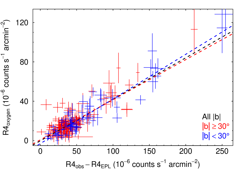
Figure 11.— R4 count-rate expected from our measured oxygen intensities against the non-EPL portion of the observed R4 count-rate, $\mathrm{R}4_{\mathrm{obs}}-\mathrm{R}4_{\mathrm{EPL}}$. We show only the results obtained using $\min(I_{\mathrm{O\,VII}})$ and $\min(I_{\mathrm{O\,VIII}})$ from directions with multiple XMM-Newton observations (see text for details). The data points are colored according to the Galactic latitude of the observation direction. The black, red, and blue dashed lines show the best-fit straight lines for all directions that have been observed multiple times, for directions with $|b|\geq 30\arcdeg$, and for directions with $|b|<30\arcdeg$, respectively.

Table 8Straight-Line Fit Results for $\mathrm{R}4_{\mathrm{oxygen}}$ against $\mathrm{R}4_{\mathrm{obs}}-\mathrm{R}4_{\mathrm{EPL}}$

Dataset	Gradient	Intercept
$\min(I)$
All $|b|$	$0.422\pm 0.024$	$-0.3\pm 1.1$
$|b|\geq 30\arcdeg$	$0.408\pm 0.039$	$+0.7\pm 1.6$
$|b|<30\arcdeg$	$0.454\pm 0.032$	$-3.1\pm 2.0$
All data, without proton flux filtering
All $|b|$	$0.485\pm 0.011$	$+1.2\pm 0.5$
$|b|\geq 30\arcdeg$	$0.509\pm 0.016$	$+1.4\pm 0.7$
$|b|<30\arcdeg$	$0.477\pm 0.014$	$-0.4\pm 0.8$
All data, with proton flux filtering
All $|b|$	$0.483\pm 0.012$	$+0.2\pm 0.6$
$|b|\geq 30\arcdeg$	$0.503\pm 0.017$	$+0.2\pm 0.7$
$|b|<30\arcdeg$	$0.479\pm 0.020$	$-1.1\pm 1.1$

Note. — Each value is the median $\pm$ the median absolute deviation of the relevant marginalized posterior probability distribution.

Clearly $\mathrm{R}4_{\mathrm{oxygen}}$ is well correlated with $\mathrm{R}4_{\mathrm{obs}}-\mathrm{R}4_{\mathrm{EPL}}$. We fitted straight lines to the data, using the method described in Section 8 of Hogg et al. (2010) for data with errors on the $x$ and $y$ values and intrinsic scatter. We used a Metropolis-Hastings Markov Chain Monte Carlo method (e.g., Press et al., 2007, Section 15.8) to sample the parameter space. We defined the “best-fit” line using the medians of the gradient and the intercept from the marginalized posterior probability distributions, with uncertainties given by the median absolute deviations of these distributions. The best-fit lines for all directions that have been observed multiple times, and for directions with $|b|\geq 30\arcdeg$ and with $|b|<30\arcdeg$, are plotted in Figure 11 in different colors, and the best-fit values are shown in Table 8.

Although not shown in plots (which would be rather crowded), we also fit straight lines to the larger datasets composed of all measurements, except for those from observations identified as SWCX-contaminated by Carter et al. (2011). We carried out two versions of these fits, one using the measurements obtained without proton flux filtering, and the other using measurements obtained with this filtering. Table 8 also contains the best-fit values from these fits.

The gradients in Table 8 imply that $\sim$40–50% of the non-EPL portion of the R4 count-rate is due to the oxygen K$\alpha$ lines. This fraction is lower when we use the $\min(I)$ oxygen intensities than when we use all of the oxygen intensities. This is unsurprising, as when we use the $\min(I)$ measurements we discard the measurements that would yield larger values of $\mathrm{R}4_{\mathrm{oxygen}}/(\mathrm{R}4_{\mathrm{obs}}-\mathrm{R}4_{\mathrm{EPL}})$. For all the fits, the intercepts are generally consistent with zero, implying that the fraction of the non-EPL R4 count-rate due to oxygen is independent of $\mathrm{R}4_{\mathrm{oxygen}}$ and $\mathrm{R}4_{\mathrm{obs}}-\mathrm{R}4_{\mathrm{EPL}}$. This implies that the spectrum of the non-EPL 3/4 keV emission does not vary systematically with its brightness. Finally, we note that the fraction of the non-EPL R4 count-rate due to oxygen is similar for low and high Galactic latitudes.

For comparison, McCammon et al. (2002) obtained a high-spectral-resolution microcalorimeter spectrum of the SXRB, and found that 52% of the R4 emission at high Galactic latitudes not due to AGN is due to the oxygen K$\alpha$ lines, which they observed at their laboratory wavelengths. The gradients in Table 8 obtained for all observations with $|b|\geq 30\arcdeg$ (with or without proton flux filtering) are in excellent agreement with this fraction. In contrast, the gradient obtained from the $\min(I)$ measurements with $|b|\geq 30\arcdeg$ is significantly smaller than the McCammon et al. (2002) fraction. These results most likely mean that the brightness of the SWCX oxygen emission in McCammon et al.’s spectrum is similar to that in a typical XMM-Newton spectrum, whereas the XMM-Newton spectra that yielded the $\min(I)$ measurements typically contain less SWCX emission than McCammon et al.’s spectrum.

4.2.3 Implications for Sources of SXRB Emission

Here we will compare the observed fraction of the non-EPL 3/4 keV SXRB due to the oxygen lines with the fractions expected from different sources. We will show that the observed values are lower than those expected from collisional ionization equilibrium (CIE) plasma in the halo, or from SWCX. Hence, it is possible that the true SWCX emission is harder than the model SWCX spectrum we have used, that the halo is out of equilibrium, and/or that oxygen is depleted in the halo.

For this comparison, it will be helpful to plot the observed fractions against $N_{\mathrm{H}}$, as the fraction expected from hot plasma in the halo varies with $N_{\mathrm{H}}$ (see below). We do this in Figure 12. The XMM-Newton observations are color-coded according to solar cycle phase, using the definitions introduced in Section 4.1.1, above (as noted earlier, the RASS was carried out during a solar maximum). As in Figure 11, we just show the results obtained using $\min(I_{\mathrm{O\,VII}})$ and $\min(I_{\mathrm{O\,VIII}})$ from directions with multiple XMM-Newton observations.

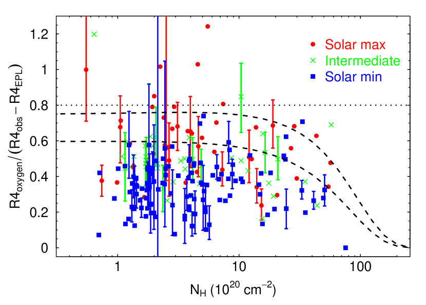
Figure 12.— Fraction of the non-EPL portion of the ROSAT R4 count-rate that is due to the oxygen K$\alpha$ lines, as a function of the H I column density, $N_{\mathrm{H}}$ (Kalberla et al., 2005). We just show the results obtained using $\min(I_{\mathrm{O\,VII}})$ and $\min(I_{\mathrm{O\,VIII}})$ from directions with multiple XMM-Newton observations (see text for details). For clarity, only a subset of the data points’ error bars are plotted. The data are color-coded according to the phases of the solar cycle during which the XMM-Newton observations were carried out (see Section 4.1.1). The upper and lower dashed curves show the expected R4 fraction for a single-temperature CIE halo plasma of temperature $2\times 10^{6}$ and $3\times 10^{6}~{}\mbox{K}$, respectively. The horizontal dotted line shows the approximate R4 fraction expected for SWCX emission.

Fractions of R4 Emission Due to Oxygen Expected from Halo Plasma and from SWCX

The dashed curves in Figure 12 show how $\mathrm{R}4_{\mathrm{oxygen}}/(\mathrm{R}4_{\mathrm{obs}}-\mathrm{R}4_{\mathrm{EPL}})$ would vary with $N_{\mathrm{H}}$ if the non-EPL 3/4 keV emission were dominated by emission from a 2 or $3\times 10^{6}~{}\mbox{K}$ plasma in CIE in the Galactic halo. Note that these model values decrease toward large $N_{\mathrm{H}}$. This is because the photoelectric absorption cross-section increases with decreasing photon energy, and so as $N_{\mathrm{H}}$ increases, the lower-energy emission in the R4 band (including the oxygen lines) is attenuated more than the higher-energy emission.

Even though we are using the $\min(I)$ measurements, SWCX may still be contributing to the 3/4 keV SXRB emission. To estimate the fraction of the R4 count-rate from a typical SWCX spectrum due to the oxygen K$\alpha$ lines, we use the spectrum shown in Figure 2 of Koutroumpa et al. (2009b). The line intensities for both solar minimum and solar maximum shown in this plot imply that $\approx$80% of the SWCX R4 count-rate is due to the oxygen K$\alpha$ lines (horizontal dotted line in Figure 12), which is slightly larger than the fraction expected from CIE plasma in the halo for $N_{\mathrm{H}}\lesssim\mathrm{few}\times 10^{21}~{}\mbox{cm}^{-2}$. We obtain similar fractions if we use the SWCX spectrum shown in Figure 1 of Koutroumpa et al. (2009c), or if we calculate the relative intensities of SWCX lines in the R4 band using cross-sections for C V, C VI, N V, N VII, O VII, O VIII lines from Table 8.2 of Bodewits (2007) and for Ne IX and Mg XI lines from Table 1 of Koutroumpa et al. (2006), with ion abundances also from Table 1 of Koutroumpa et al. (2006).

The observed values of $\mathrm{R}4_{\mathrm{oxygen}}/(\mathrm{R}4_{\mathrm{obs}}-\mathrm{R}4_{\mathrm{EPL}})$ are generally much lower than those expected from a $\sim$$(\mbox{2--3})\times 10^{6}~{}\mbox{K}$ CIE plasma in the halo, or from SWCX emission. Hence, a combination of these two emission mechanisms seems to be unable to explain the observed values of $\mathrm{R}4_{\mathrm{oxygen}}/(\mathrm{R}4_{\mathrm{obs}}-\mathrm{R}4_{\mathrm{EPL}})$. In the remainder of this subsection we will explore possible explanations for the low observed values of $\mathrm{R}4_{\mathrm{oxygen}}/(\mathrm{R}4_{\mathrm{obs}}-\mathrm{R}4_{\mathrm{EPL}})$.

Is the SWCX Emission Fainter in the XMM-Newton Data than in the ROSAT Data?

Here, we consider the possibility that the SWCX emission (specifically, the oxygen emission) is typically fainter in the XMM-Newton observations than it was during the RASS; i.e., the values of $\mathrm{R}4_{\mathrm{oxygen}}$ derived from the XMM-Newton data may be smaller than the values we would have obtained had we been able to measure $\mathrm{R}4_{\mathrm{oxygen}}$ at the same time as $\mathrm{R}4_{\mathrm{obs}}-\mathrm{R}4_{\mathrm{EPL}}$. Such an occurrence would have the effect of lowering the $\mathrm{R}4_{\mathrm{oxygen}}/(\mathrm{R}4_{\mathrm{obs}}-\mathrm{R}4_{\mathrm{EPL}})$ ratio. This explanation for the low observed ratios is plausible because the XMM-Newton observations that yield low values of $\mathrm{R}4_{\mathrm{oxygen}}/(\mathrm{R}4_{\mathrm{obs}}-\mathrm{R}4_{\mathrm{EPL}})$ were typically taken during solar minimum, while the RASS was carried out during solar maximum, and, as we showed in Section 4.1.1, the oxygen intensities are typically fainter during solar minimum than during solar maximum (see Figure 9). However, it should be noted that a few XMM-Newton observations taken during solar maximum (i.e., the equivalent phase as the RASS) also yield low values of $\mathrm{R}4_{\mathrm{oxygen}}/(\mathrm{R}4_{\mathrm{obs}}-\mathrm{R}4_{\mathrm{EPL}})$. Furthermore, when we examine this explanation more quantitatively, we find that it is unable to reproduce the observed values of $\mathrm{R}4_{\mathrm{oxygen}}/(\mathrm{R}4_{\mathrm{obs}}-\mathrm{R}4_{\mathrm{EPL}})$ for XMM-Newton observations taken during solar minimum, as we will now demonstrate.

We begin by defining $\mathrm{R}4_{\mathrm{SWCX}}$ and $\mathrm{R}4_{\mathrm{halo}}$ as the contributions to the RASS R4 count-rate from SWCX and the halo, respectively; i.e., $\mathrm{R}4_{\mathrm{obs}}-\mathrm{R}4_{\mathrm{EPL}}=\mathrm{R}4_{\mathrm{SWCX}}+\mathrm{R}4_{\mathrm{halo}}$ (we are assuming the contribution from the LB is negligible). Note that $\mathrm{R}4_{\mathrm{SWCX}}$ is the count-rate due to SWCX during solar maximum. If $\gamma_{\mathrm{SWCX}}$ and $\gamma_{\mathrm{halo}}$ are the expected fractions of $\mathrm{R}4_{\mathrm{SWCX}}$ and $\mathrm{R}4_{\mathrm{halo}}$, respectively, due to oxygen, and $\xi$ is the typical factor by which oxygen SWCX intensities are reduced in going from solar maximum (epoch of the RASS) to solar minimum (blue data points in Figure 12), then a typical value of $\mathrm{R}4_{\mathrm{oxygen}}$ for an XMM-Newton observation taken during solar minimum would be given by

$$\mathrm{R}4_{\mathrm{oxygen}}=\xi\gamma_{\mathrm{SWCX}}\mathrm{R}4_{\mathrm{SWCX}}+\gamma_{\mathrm{halo}}\mathrm{R}4_{\mathrm{halo}}.$$ (6)

Since $\gamma_{\mathrm{SWCX}}\approx 0.8$ and $\gamma_{\mathrm{halo}}\approx 0.7$ (see Figure 12),

$$\frac{\mathrm{R}4_{\mathrm{oxygen}}}{\mathrm{R}4_{\mathrm{obs}}-\mathrm{R}4_{\mathrm{EPL}}}\approx 0.8(1-f)\xi+0.7f,$$ (7)

where $f\equiv\mathrm{R}4_{\mathrm{halo}}/(\mathrm{R}4_{\mathrm{obs}}-\mathrm{R}4_{\mathrm{EPL}})$ is the typical fraction of the EPL-subtracted R4 count-rate that is from the halo. For the R45 band, Table 2 in Kuntz & Snowden (2000) implies that 78% of the count-rate not due to the EPL or point sources is from the halo. An equivalent measurement for the R4 band is not available, but using the temperatures and normalizations of the relevant model components from Kuntz & Snowden (2000), we estimate that $f\approx 0.7$.

For the observations taken during solar minimum, $\mathrm{R}4_{\mathrm{oxygen}}/(\mathrm{R}4_{\mathrm{obs}}-\mathrm{R}4_{\mathrm{EPL}})$ is typically 0.24–0.44 (these are the lower and upper quartiles, respectively). For $f\approx 0.7$, we find that Equation (7) can only yield $\mathrm{R}4_{\mathrm{oxygen}}/(\mathrm{R}4_{\mathrm{obs}}-\mathrm{R}4_{\mathrm{EPL}})=0.24$–0.44 if $\xi<0$, which is unphysical. Hence, while the lower oxygen SWCX intensities during solar minimum may be partly responsible for the low observed values of $\mathrm{R}4_{\mathrm{oxygen}}/(\mathrm{R}4_{\mathrm{obs}}-\mathrm{R}4_{\mathrm{EPL}})$, they do not fully explain the observations. Also, as noted above, a few XMM-Newton observations taken during solar maximum also yield low values of $\mathrm{R}4_{\mathrm{oxygen}}/(\mathrm{R}4_{\mathrm{obs}}-\mathrm{R}4_{\mathrm{EPL}})$.

Is the Halo Much Hotter than $\mathit{\sim}$$\mathit{3\times 10^{6}~{}\mbox{K}}$?

For a CIE plasma with $T\gtrsim 2\times 10^{6}~{}\mbox{K}$, $\mathrm{R}4_{\mathrm{oxygen}}/(\mathrm{R}4_{\mathrm{obs}}-\mathrm{R}4_{\mathrm{EPL}})$ is expected to decrease with increasing temperature (e.g., compare the curves for $T=2$ and $3\times 10^{6}~{}\mbox{K}$ in Figure 12). This is because, as the temperature increases, the harder emission in the R4 band brightens relative to the oxygen emission. However, the low observed values of $\mathrm{R}4_{\mathrm{oxygen}}/(\mathrm{R}4_{\mathrm{obs}}-\mathrm{R}4_{\mathrm{EPL}})$ are unlikely to mean that the halo temperature is much greater than $3\times 10^{6}~{}\mbox{K}$. Such a high temperature would exceed the Galaxy’s virial temperature (e.g., Bregman, 2009), and the hot halo gas would escape from the Galaxy’s potential well.

It should also be noted that some observations that have yielded typical halo temperatures elsewhere yield low values of $\mathrm{R}4_{\mathrm{oxygen}}/(\mathrm{R}4_{\mathrm{obs}}-\mathrm{R}4_{\mathrm{EPL}})$ here. For example, 22 out of the 26 XMM-Newton observations studied by Henley et al. (2010) yielded halo temperatures between $1.5\times 10^{6}$ and $2.5\times 10^{6}~{}\mbox{K}$, assuming CIE. Of these 22 observations, 14 yield $\mathrm{R}4_{\mathrm{oxygen}}/(\mathrm{R}4_{\mathrm{obs}}-\mathrm{R}4_{\mathrm{EPL}})<0.5$.

We have excluded differences in the SWCX oxygen intensities between the RASS data and the XMM-Newton data, and a very high halo temperature as possible explanations for the low observed values of $\mathrm{R}4_{\mathrm{oxygen}}/(\mathrm{R}4_{\mathrm{obs}}-\mathrm{R}4_{\mathrm{EPL}})$. In the following paragraphs, we consider three further explanations that we cannot exclude. Currently, we cannot discriminate between these proposed explanations.

Is the SWCX Emission Harder than Expected?

It is possible that the true SWCX spectrum is harder than the model SWCX spectra we have used, which would mean that $\gamma_{\mathrm{SWCX}}\approx 0.8$ is an overestimate. This could arise from inaccuracies in the assumed charge exchange cross-sections or ion fractions. If there were relatively more flux from lines with energies greater than those of the oxygen K$\alpha$ lines, it would help explain the low observed values of $\mathrm{R}4_{\mathrm{oxygen}}/(\mathrm{R}4_{\mathrm{obs}}-\mathrm{R}4_{\mathrm{EPL}})$.

Is the Halo out of Equilibrium?

It is also possible that the true halo spectrum is harder than that expected from a $\sim$$(\mbox{2--3})\times 10^{6}~{}\mbox{K}$ CIE plasma. We ruled out above the possibility that the halo temperature is much greater than $3\times 10^{6}~{}\mbox{K}$. Instead, these results may imply that the halo is overionized and recombining (Breitschwerdt & Schmutzler, 1994, 1999). The emission from an overionized, recombining plasma may include relatively bright recombination continuum emission at higher energies than the oxygen lines. Hence, the fraction of the EPL-subtracted R4 emission due to oxygen may be lower than that expected from a few-million-degree CIE plasma, as observed. If this is true, it would have important implications for spectral analyses of the halo, as it suggests that CIE halo models with best-fit temperatures of $\sim$$(\mbox{2--3})\times 10^{6}~{}\mbox{K}$ (e.g., Galeazzi et al., 2007; Lei et al., 2009; Yoshino et al., 2009; Gupta et al., 2009; Henley et al., 2010) may not accurately model the higher-energy emission from the halo.

Is Oxygen Depleted in the Halo?

When calculating the values of $\mathrm{R}4_{\mathrm{oxygen}}/(\mathrm{R}4_{\mathrm{obs}}-\mathrm{R}4_{\mathrm{EPL}})$ expected from a hot halo plasma (Figure 12), we assumed solar abundances (Anders & Grevesse, 1989). However, it is possible that oxygen is depleted in the halo. Yoshino et al. (2009) found evidence from a subset of their Suzaku observations that neon and iron are enhanced in the halo relative to oxygen. If oxygen were depleted in the halo, $\mathrm{R}4_{\mathrm{oxygen}}/(\mathrm{R}4_{\mathrm{obs}}-\mathrm{R}4_{\mathrm{EPL}})$ would be lower than expected for a solar-abundance plasma, which is what we observe. If oxygen is underabundant in the halo then, similarly to above, models that assume solar abundances (e.g., Galeazzi et al., 2007; Lei et al., 2009; Gupta et al., 2009; Henley et al., 2010) may not accurately model the halo’s higher-energy emission.

4.3. Spatial Variation of the Oxygen Intensities

Figure 13.— Kendall’s $\tau$ correlation coefficients for $I_{\mathrm{O\,VII}}$ (left) and $I_{\mathrm{O\,VIII}}$ (right) against $l$ for directions with $0\arcdeg\leq l<180\arcdeg$ or against $360\arcdeg-l$ for directions with $180\arcdeg\leq l<360\arcdeg$, for different regions of the sky. The upper pair of plots shows the results for intensities obtained with proton flux filtering (observations identified as SWCX-contaminated by Carter et al. (2011) are excluded, as are observations toward the Eridanus enhancement and the Magellanic Clouds). The lower pair of plots show the results for directions with multiple XMM-Newton observations, using the minimum intensity measured in each direction (again, observations toward the Eridanus enhancement and the Magellanic Clouds are excluded). The uncertainties indicate the 90% confidence interval on $\tau$ obtained by bootstrap resampling. The results are generally shown in boldface; the one case for which the confidence interval encompasses zero is shown in italics.

The variation of the oxygen intensities with Galactic longitude and latitude can provide information on the general geometry of the halo. This, in turn, provides information on the mechanism responsible for heating the hot halo gas. For example, if the heating of the halo is dominated by SN-driven outflows from the disk (e.g., Shapiro & Field, 1976; Bregman, 1980; Joung & Mac Low, 2006; Henley et al., 2010), and the SN rate per unit area of the disk is fairly uniform in the vicinity of the Sun, then we would expect an approximately plane-parallel geometry for the halo, with the same intrinsic halo brightness for all longitudes. If the SN rate increases toward the Galactic Center, we would expect the halo brightness to increase toward the inner Galaxy. An increase in the halo brightness toward the inner Galaxy may also indicate that a halo of accreted extragalactic material centered on the Galactic Center (e.g., Crain et al., 2010) is contributing to the halo emission.

In practice it is difficult to determine the true halo geometry from our intensity measurements, because of the unknown amount of SWCX emission contributing to each measurement. However, we can gain some insight by looking for correlations between the observed intensities and Galactic longitude and latitude. As we do not expect the SWCX intensity to be correlated with Galactic longitude and latitude, any observed correlations most likely reflect variations in the observed halo intensity, which may be due to variations in the intrinsic intensity or in $N_{\mathrm{H}}$.

In Sections 4.3.1 and 4.3.2 we will examine the variation of the observed intensities with Galactic longitude and latitude, respectively. Then, in Section 4.3.3, we will compare the observed variation with Galactic latitude with the variation expected from simple models of the intrinsic halo emission, in an attempt to constrain the variation of the intrinsic halo intensity with latitude.

4.3.1 Variation with Galactic Longitude

Figure 13 show the correlation coefficients (Kendall’s $\tau$; e.g., Press et al. 1992) for the observed intensities against $l$ for directions with $0\arcdeg\leq l<180\arcdeg$ or against $360\arcdeg-l$ for directions with $180\arcdeg\leq l<360\arcdeg$, for different regions of the sky. In the top panels, we use the intensities obtained with proton flux filtering, and exclude observations identified as SWCX-contaminated by Carter et al. (2011), as well as observations toward the Eridanus enhancement (e.g., Burrows et al., 1993; Snowden et al., 1995a) and the Magellanic Clouds. We calculate the 90% confidence intervals on the correlation coefficients by bootstrap resampling. In the upper pair of plots, all of the correlation coefficients are significantly different from zero; they are shown in boldface print.

There is a clear tendency for the observed O VII and O VIII intensities to increase from the outer Galaxy ($l=180\arcdeg$) to the inner Galaxy ($l=0\arcdeg$ or 360°); see also Figure 2. This trend is seen at all latitudes. However, we discount the trend seen at high latitudes in the northern Galactic hemisphere, as it is likely due to the presence of the Scorpius-Centaurus (Sco-Cen) superbubble (Egger & Aschenbach, 1995) toward the inner Galaxy, and so does not tell us anything about the halo. Similarly, the trends at low latitudes reflect variations in the disk, rather than the halo. However, the trends seen toward high southern latitudes most likely reflect real variation in the observed Galactic halo intensity, a conclusion that is supported by the fact that the trends are generally still apparent when we use only $\min(I_{\mathrm{O\,VII}})$ or $\min(I_{\mathrm{O\,VIII}})$ (the lower pair of panels in Figure 13; in only one case is the correlation coefficient consistent with zero, and this is shown in italics in the figure). As $N_{\mathrm{H}}$ is not correlated with $l$ in this region of the sky, these results imply that the intrinsic halo intensity increases from the outer to the inner Galaxy. As noted above, this increase may indicate an increase in the SN rate toward the inner Galaxy or the presence of a halo of accreted extragalactic material centered on the Galactic Center.

             

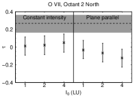
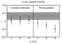
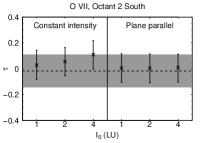
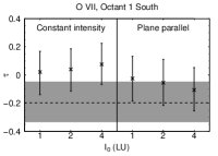
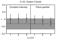
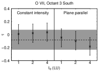
Figure 14.— Central upper panel: Kendall’s $\tau$ correlation coefficients for $I_{\mathrm{O\,VII}}$ (obtained with proton flux filtering) against $|b|$, for different regions of the sky. We consider only sightlines with $|b|\geq 30\arcdeg$, and exclude observations identified as SWCX-contaminated by Carter et al. (2011), or that are toward the Eridanus enhancement or the Magellanic Clouds. The uncertainties indicate the 90% confidence interval on $\tau$ obtained by bootstrap resampling; if this interval does not (does) encompass zero, the results are shown in boldface (italics). Surrounding panels: Comparisons of the observed correlation coefficients with those expected from different halo models, for six different regions of the sky. In each panel, the horizontal dashed line shows the observed value of $\tau$, with the gray band indicating the 90% bootstrap confidence interval. The errorbars indicate the 90% confidence intervals on the values of $\tau$ predicted by different halo models. The left half of each panel shows the predictions for models in which the intrinsic halo intensity is the same in all directions, while the right half of each panel shows the predictions for plane parallel halo models, in which the intrinsic halo intensity varies as $\mathrm{cosec}\,|b|$. For each model, we show predictions for different model normalizations, $I_{0}$, indicated on the $x$-axis. See the text for the details of how these model predictions were generated. Note that we do not show results for the 1st and 4th northern octants ($0\arcdeg\leq l<90\arcdeg$ and $270\arcdeg\leq l<360\arcdeg$, respectively), because of the presence of the Sco-Cen superbubble in this region of the sky.

             

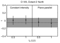
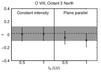
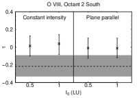
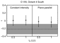
Figure 15.— As Figure 14, but for O VIII. Note that the values of $I_{0}$ used to model the correlation coefficients here are different from those used in Figure 14.

4.3.2 Variation with Galactic Latitude

The central upper panels in Figure 14 (O VII) and Figure 15 (O VIII) show the correlation coefficients for the observed intensities against $|b|$, for different regions of the sky with $|b|\geq 30\arcdeg$. As in the upper panels of Figure 13, we use the intensities obtained with proton flux filtering, and exclude observations identified as SWCX-contaminated by Carter et al. (2011), as well as observations toward the Eridanus enhancement and the Magellanic Clouds. As in Figure 13, the correlations that are significantly different from zero are in boldface print, and those that are consistent with zero are in italics.

The correlations between intensity and $|b|$ vary significantly across the sky. However, some general trends do emerge. In the 1st and 4th northern octants ($0\arcdeg\leq l<90\arcdeg$ and $270\arcdeg\leq l<360\arcdeg$, respectively), the O VIII intensities are generally anticorrelated with $|b|$ (i.e., the observed intensities tend to decrease toward the northern Galactic pole), while the O VII intensities are not significantly correlated with $|b|$. However, as this region of the sky is dominated by emission from the Sco-Cen superbubble, these trends do not tell us anything about the halo. In the 2nd and 3rd northern octants, the O VII intensities are positively correlated with $|b|$, while the O VIII intensities are not significantly correlated with $|b|$. In the southern hemisphere, the intensities are either anticorrelated with $|b|$ (i.e., they tend to decrease toward the southern Galactic pole), or are not significantly correlated with $|b|$. In general, the O VII and O VIII lines behave differently (i.e., in most southern octants, only one of O VII or O VIII is significantly anticorrelated with $|b|$).

4.3.3 Modeling the Variation with Galactic Latitude

In an attempt to constrain the geometry of the intrinsic halo emission, here we compare the observed correlation coefficients with the correlation coefficients that we would expect to observe from each of two different halo models. We use the correlation coefficients, instead of fitting halo models directly to the observed intensities, because the uncertainty in the contribution from SWCX to each intensity measurement prevents us from using standard least-squares fitting techniques.

In brief, we simulated many datasets in which each simulated intensity is the sum of the absorbed model halo emission intensity, a SWCX intensity (which is randomly chosen from the observed $I-\min(I)$ distribution in order to mimic the unpredictability of time-variable SWCX emission), and a measurement error. See below for details. We then calculate the correlation coefficient between the model intensities and Galactic latitude for each simulated dataset, expecting that the random time-variable SWCX emission will “blur” the correlation coefficient expected from the underlying halo emission. Having done this procedure for many simulated datasets, we obtain a distribution of simulated correlation coefficients, which we then compare with the observed correlation coefficient (in particular, the distribution obtained by bootstrap resampling the observations, which indicates the uncertainty on the observed correlation coefficient). Essentially, we are asking which halo model(s) can reproduce the observed correlation coefficients, in the presence of the “blurring” effect of the time-variable SWCX emission. Our method is described in more detail below.

Modeling the Correlation Coefficients for Different Halo Models

For a given region of the sky, and for a given halo model, we generated 1000 sets of simulated intensity measurements for each line (O VII and O VIII). Within each of these sets, the latitudes and column densities of the simulated observations matched those of the actual observations in that region of sky (we restricted ourselves to the observations that yielded oxygen measurements after being subjected to the proton flux filtering; Table 2). As noted above, each simulated intensity measurement was the sum of the absorbed model halo emission, a randomly chosen intensity due to the time-variable SWCX emission, and a randomly chosen positive or negative intensity that mimics the measurement error. We examined two halo models: a plane-parallel model, in which the intrinsic halo intensity is given by $I_{0}\mathrm{cosec}\,|b|$, and a constant-intensity model, in which the intrinsic halo intensity, $I_{0}$, is independent of $b$. For each model we tested different values of $I_{0}$ – the smaller the value of $I_{0}$, the more likely it is that any potentially observable correlation due to the halo is obscured by the SWCX emission or the measurement error. We assumed that the intensity of the time-variable SWCX emission followed the distribution given by our $I-\min(I)$ measurements from the proton-flux-filtered data (gray histograms in Figures 6(c) and 6(d)). Note that our model considers only the time-variable SWCX emission. We are implicitly assuming that any non-variable SWCX emission does not vary strongly with Galactic latitude, and hence does not affect the correlation coefficient between intensity and latitude.

Therefore, for the plane-parallel model, the $j$th simulated O VII or O VIII intensity (for $j=1$ to 1000) corresponding to the $i$th actual observation (where $i=1$ to $N$, $N$ being the number of observations in the region of the sky being studied) is given by

$$I_{\mathrm{sim},ij}=I_{0}\mathrm{cosec}\,|b_{i}|\mathrm{e}^{-\sigma{N_{\mathrm{H}}}_{i}}+I_{\mathrm{SWCX},ij}+\epsilon_{ij},$$ (8)

and for the constant-intensity model it is given by

$$I_{\mathrm{sim},ij}=I_{0}\mathrm{e}^{-\sigma{N_{\mathrm{H}}}_{i}}+I_{\mathrm{SWCX},ij}+\epsilon_{ij}.$$ (9)

Here, $b_{i}$ is the Galactic latitude of the $i$th actual observation, ${N_{\mathrm{H}}}_{i}$ is the column density in the direction of this observation (Kalberla et al., 2005), $\sigma$ is the photoelectric absorption cross-section appropriate for the emission line energy in question (Bałucińska-Church & McCammon, 1992; Yan et al., 1998), $I_{\mathrm{SWCX},ij}$ is the simulated SWCX intensity for this simulated observation, and $\epsilon_{ij}$ represents the measurement error. As noted above, the values of $I_{\mathrm{SWCX},ij}$ were drawn randomly from a distribution that follows the observed $I-\min(I)$ distribution for the line in question (gray histograms in Figures 7(c) and 7(d) for O VII and O VIII, respectively). The values of $\epsilon_{ij}$ were drawn randomly from a zero-mean normal distribution with standard deviations of 1.7 and 1.2 L.U. for O VII and O VIII, respectively (these are the 75th percentiles of the observed statistical + systematic measurement errors).

We created such datasets for each octant of the sky, except for the 1st and 4th northern octants. We omitted these regions because of the presence of the Sco-Cen superbubble. As we are interested in the halo, we considered only high Galactic latitudes ($|b|\geq 30\arcdeg$).

For each simulated dataset, we calculated the correlation coefficient for the intensity against $|b|$. For each choice of oxygen emission line, halo model, and sky octant, the set of calculated correlation coefficients forms a distribution. These distributions of simulated correlation coefficients for O VII are summarized by the errorbars in Figure 14 – the results for the constant-intensity and plane-parallel halo models are shown in the left and right halves of each panel, respectively, for different values of model $I_{0}$, as indicated on the $x$-axes. Each errorbar indicates the 5th and 95th percentile of a given distribution of simulated correlation coefficients, while the crosses indicate the medians. The corresponding results for O VIII are shown in Figure 15. Note that the values of $I_{0}$ used to model the O VII and O VIII correlation coefficients differ – larger values of $I_{0}$ tend to overpredict the O VIII intensities. For O VIII, we find that we generally cannot distinguish between the models. This is likely because the differences in the intensities predicted by the various models are small compared to the uncertainties due to the SWCX emission and the measurement error. Finally, note that, because the variation of $N_{\mathrm{H}}$ with $b$ is not the same in all octants, the same model may produce different correlation coefficients in different octants.

Comparison with Observations

For each octant of the sky in Figures 14 and 15 for which we have calculated model predictions, we have overplotted the observed correlation coefficient as a horizontal dashed line, with a horizontal gray band indicating the 90% confidence interval. Here, we visually compare the above-described model predictions with the observed correlation coefficients.

No single model compares well with the observed correlation coefficients in all octants for both O VII and O VIII. Both halo models are generally in agreement with the observed O VII correlation coefficients in the four southern octants, although in the 1st southern quadrant, the plane-parallel model may be favored over the constant-intensity model, and in the 2nd southern octant, the plane-parallel model with $I_{0}=4~{}\mbox{L.U.}$ tends to systematically overpredict the intensities at lower latitudes (not plotted). However, only the constant-intensity model is in good agreement with the observed correlation coefficient in the 3rd northern octant, and neither model agrees with the observed correlation coefficient in the 2nd northern octant.

For O VIII, both halo models are generally in agreement with the observed correlation coefficients. The exception is the 2nd southern quadrant, in which neither model agrees well with the observed correlation coefficient.

The most important result from this analysis is that no single halo model seems to be able to account for the observed variation in intensity with Galactic latitude in all directions. Some octants seem to favor the plane-parallel geometry, others seem to favor a constant-intensity model, while in others neither model is in good agreement with the data. Determining the true halo intensity, and hence the true halo geometry, however, will require a better method for disentangling the halo and SWCX contributions to the observed emission.

5. SUMMARY

We have presented a new catalog of SXRB O VII and O VIII intensities, extracted from 1880 archival XMM-Newton observations. This catalog covers the full range of Galactic longitudes, and supersedes our previous catalog (Paper I), which covered $l=120\arcdeg$–240°. Our new analysis has some improvements over our previous analysis, including the use of more recent software and calibration data, the use of data from the XMM-Newton Serendipitous Source Catalogue for point source removal, and the estimation of the systematic errors on the oxygen intensities (see Section 3.5 for more details on the differences from Paper I).

As in Paper I, we attempted to reduce the affects of SWCX contamination by excluding the portions of the XMM-Newton observations for which the contemporaneous solar wind proton flux exceeded $2\times 10^{8}~{}\mbox{cm}^{-2}\ \mbox{s}^{-1}$. Of the 1880 XMM-Newton observations for which we have results, 1868 yielded oxygen intensities without the proton flux filtering, and 1003 yielded results with this filtering. In practice, the proton flux filtering tended to render unusable those observations that yielded particularly bright oxygen intensities (i.e., the solar wind proton flux tended to exceed our threshold of $2\times 10^{8}~{}\mbox{cm}^{-2}\ \mbox{s}^{-1}$ during such observations). As a result, the set of filtered observations generally yields lower oxygen intensities than the set of unfiltered observations. However, among the set of observations for which the proton flux filtering did remove at least some XMM-Newton data, but not so much that the observation became unusable, we found that the filtered observations did not yield systematically lower oxygen intensities than the unfiltered observations (see Section 3.7).

Our main results were presented in Section 3.3. We found a large range of intensities: 0.0–50.8 and 0.0–36.2 L.U. for O VII and O VIII, respectively, for intensities obtained without proton flux filtering (0.0–48.8 and 0.0–24.5 L.U., respectively, for intensities obtained with this filtering). However, the typical O VII and O VIII intensities are $\sim$2–11 and $\lesssim$3 L.U., respectively. Note that we excluded bright diffuse objects such as SN remnants or galaxy clusters during our processing, so the brightest intensities that we measured should not be contaminated by emission from such objects. The medians and quartiles of the oxygen intensities are generally significantly higher than those in Paper I, as the current paper includes observations toward the inner Galaxy, which typically yield higher intensities. We also found that the observations identified by Carter et al. (2011) as being contaminated by SWCX emission tended to yield larger-than-typical oxygen intensities.

Our dataset includes measurements for 217 sightlines that have been observed more than once with XMM-Newton (see Section 3.4). For a given direction, the differences in the measured oxygen intensities between observations can be attributed to the time-variable SWCX emission. Typically, the variations in the O VII and O VIII intensities are $\lesssim$5 and $\lesssim$2 L.U., respectively. However, some observations exhibit bright intensity enhancements, the brightest being an O VII enhancement of 24 L.U. over another observation in the same direction (note that this bright enhancement was also reported in Paper I).

We discussed various aspects of our results in Section 4. Some important results are as follows:

1. The oxygen intensities generally decrease from solar maximum to solar minimum, at high and low ecliptic latitudes. While this is as expected for high ecliptic latitudes from heliospheric SWCX models, it is not as expected for low ecliptic latitudes (Koutroumpa et al., 2006). We also found that the O VII intensities during solar maximum are higher toward high ecliptic latitudes, while those during solar minimum are higher toward low ecliptic latitudes (the differences are small but statistically significant). The O VIII intensities, however, do not exhibit clear variation with ecliptic latitude (see Section 4.1.1).

2. The observed variations in oxygen intensity are in poor agreement with the predictions of a geocoronal SWCX model similar to that described in Robertson & Cravens (2003b). This model takes into account the time-variable density of the solar wind in and beyond the magnetosheath, using the Spreiter et al. (1966) magnetosphere model and solar wind data from OMNIWeb. For each XMM-Newton observation, the expected geocoronal SWCX emissivity is integrated along the line of sight, taking into account the position and orientation of XMM-Newton. In Section 4.1.2 we discussed various possible reasons for the discrepancy between the model predictions and the observations.

3. Approximately $\sim$40–50% of the 3/4 keV SXRB (specifically, the ROSAT R4 count-rate) that is not due to the extragalactic background is due to the oxygen K$\alpha$ lines (see Section 4.2.2). This value is similar to the fraction derived from a high-resolution microcalorimeter spectrum of the SXRB (McCammon et al., 2002). The fraction is independent of the oxygen K$\alpha$ intensity and the non-EPL 3/4 keV surface brightness, implying that the spectrum of the non-EPL 3/4 keV emission does not vary systematically with its brightness.

4. The above fraction is less than the fraction expected if the non-EPL 3/4 keV SXRB were dominated by a combination of unabsorbed SWCX emission and absorbed emission from a $\sim$$(\mbox{2--3})\times 10^{6}~{}\mbox{K}$ CIE plasma in the halo. We ruled out the possibilities that the SWCX emission was brighter during the RASS than during the XMM-Newton observations, or that the halo is much hotter than $3\times 10^{6}~{}\mbox{K}$. Instead, these results may indicate that the true SWCX emission is harder than expected, or that the halo is out of equilibrium and overionized, or that oxygen is depleted in the halo (see Section 4.2.3). With our current measurements, we are unable to distinguish between these possibilities. However, we noted that it is possible that solar-abundance CIE models of the halo with $T\sim\mbox{(2--3)}\times 10^{6}~{}\mbox{K}$ underestimate the halo emission at energies greater than those of the oxygen K$\alpha$ lines.

5. The oxygen intensities tend to increase from the outer to the inner Galaxy, which may indicate either that the SN rate increases toward the inner Galaxy (if the hot halo gas is mainly due to Galactic fountains) or the presence of a halo of accreted material centered on the Galactic Center (see Section 4.3.1).

6. No clear overall picture emerges when we look at the variation of the intensities with Galactic latitude: some regions of the sky exhibit a statistically significant positive correlation between intensity and latitude, some regions exhibit a statistically significant anticorrelation, and some regions exhibit no significant correlation or anticorrelation (see Section 4.3.2). We compared the observed correlation coefficients with those expected from two models of the intrinsic halo emission (a constant-intensity model (intrinsic intensity independent of $b$), and a plane-parallel model) and found that no one halo model appears to be able to explain the observations in all octants. Indeed, in some octants, neither model is in good agreement with the observations (see Section 4.3.3).

Our catalog of oxygen intensities will provide useful constraints on models of the heliospheric and geocoronal SWCX emission – as noted above, the variation in the oxygen intensities measured from different observations of the same direction can be attributed to the time-variable SWCX emission. Then, equipped with suitable models of the SWCX emission, one can subtract the estimated SWCX intensity for each observation, revealing the O VII and O VIII intensities due to the hot gas in our Galaxy. From these intensities, the temperature and distribution on the sky of this hot gas can be inferred.

An alternative method for constraining the halo oxygen emission, which we are currently investigating, is to use Bayesian analysis. The observed $I-\min(I)$ distributions (Figure 6) can be used to specify the prior probability distribution for the SWCX intensity in an arbitrary XMM-Newton spectrum. Using this prior, one can then, in principle, calculate the posterior probability distribution for the halo emission intensity.

Finally, it should be noted that the XMM-Newton SXRB spectra that we have extracted contain more information than just the diffuse oxygen line intensities. For example, by fitting appropriate models to the spectra one can constrain the temperature and emission measure of the halo, and use these results to test physical models for the hot halo gas (as in Henley et al. 2010)

References

- Anders & Grevesse (1989) Anders, E., & Grevesse, N. 1989, Geochim. Cosmochim. Acta, 53, 197
- Avni (1976) Avni, Y. 1976, ApJ, 210, 642
- Bałucińska-Church & McCammon (1992) Bałucińska-Church, M., & McCammon, D. 1992, ApJ, 400, 699
- Bodewits (2007) Bodewits, D. 2007, PhD thesis, University of Groningen
- Brandt & Hasinger (2005) Brandt, W. N., & Hasinger, G. 2005, ARA&A, 43, 827
- Bregman (1980) Bregman, J. N. 1980, ApJ, 236, 577
- Bregman (2009) Bregman, J. N. 2009, in The Role of Disk-Halo Interaction in Galaxy Evolution: Outflow vs. Infall? (arXiv:0907.3494v1)
- Breitschwerdt & Schmutzler (1994) Breitschwerdt, D., & Schmutzler, T. 1994, Nature, 371, 774
- Breitschwerdt & Schmutzler (1999) Breitschwerdt, D., & Schmutzler, T. 1999, A&A, 347, 650
- Burrows & Mendenhall (1991) Burrows, D. N., & Mendenhall, J. A. 1991, Nature, 351, 629
- Burrows et al. (1993) Burrows, D. N., Singh, K. P., Nousek, J. A., Garmire, G. P., & Good, J. 1993, ApJ, 406, 97
- Carter & Sembay (2008) Carter, J. A., & Sembay, S. 2008, A&A, 489, 837
- Carter et al. (2010) Carter, J. A., Sembay, S., & Read, A. M. 2010, MNRAS, 402, 867
- Carter et al. (2011) Carter, J. A., Sembay, S., & Read, A. M. 2011, A&A, 527, A115
- Cen & Ostriker (1999) Cen, R., & Ostriker, J. P. 1999, ApJ, 514, 1
- Chen et al. (1997) Chen, L.-W., Fabian, A. C., & Gendreau, K. C. 1997, MNRAS, 285, 449
- Cox & Reynolds (1987) Cox, D. P., & Reynolds, R. J. 1987, ARA&A, 25, 303
- Crain et al. (2010) Crain, R. A., McCarthy, I. G., Frenk, C. S., Theuns, T., & Schaye, J. 2010, MNRAS, 407, 1403
- Cravens (2000) Cravens, T. E. 2000, ApJ, 532, L153
- Cravens (2002) Cravens, T. E. 2002, Science, 296, 1042
- Cravens et al. (2001) Cravens, T. E., Robertson, I. P., & Snowden, S. L. 2001, JGR, 106 (A11), 24883
- Egger & Aschenbach (1995) Egger, R. J., & Aschenbach, B. 1995, A&A, 294, L25
- Ezoe et al. (2010) Ezoe, Y., Ebisawa, K., Yamasaki, N. Y., et al. 2010, PASJ, 62, 981
- Ezoe et al. (2011) Ezoe, Y., Miyoshi, Y., Yoshitake, H., et al. 2011, PASJ, 63, S691
- Fujimoto et al. (2007) Fujimoto, R., Mitsuda, K., McCammon, D., et al. 2007, PASJ, 59, S133
- Galeazzi et al. (2007) Galeazzi, M., Gupta, A., Covey, K., & Ursino, E. 2007, ApJ, 658, 1081
- Garmire et al. (1992) Garmire, G. P., Nousek, J. A., Apparao, K. M. V., et al. 1992, ApJ, 399, 694
- Geyer (2010) Geyer, C. J. 2010, mcmc: Markov Chain Monte Carlo, R package version 0.8 (http://CRAN.R-project.org/package=mcmc)
- Gupta et al. (2009) Gupta, A., Galeazzi, M., Koutroumpa, D., Smith, R., & Lallement, R. 2009, ApJ, 707, 644
- Henley & Shelton (2008) Henley, D. B., & Shelton, R. L. 2008, ApJ, 676, 335
- Henley & Shelton (2010) Henley, D. B., & Shelton, R. L. 2010, ApJS, 187, 388 (Paper I)
- Henley et al. (2010) Henley, D. B., Shelton, R. L., Kwak, K., Joung, M. R., & Mac Low, M.-M. 2010, ApJ, 723, 935
- Hogg et al. (2010) Hogg, D. W., Bovy, J., & Lang, D. 2010, arXiv:1008.4686
- Jansen et al. (2001) Jansen, F., Lumb, D., Altieri, B., et al. 2001, A&A, 365, L1
- Joung & Mac Low (2006) Joung, M. K. R., & Mac Low, M.-M. 2006, ApJ, 653, 1266
- Kalberla et al. (2005) Kalberla, P. M. W., Burton, W. B., Hartmann, D., et al. 2005, A&A, 440, 775
- Koutroumpa et al. (2007) Koutroumpa, D., Acero, F., Lallement, R., Ballet, J., & Kharchenko, V. 2007, A&A, 475, 901
- Koutroumpa et al. (2009a) Koutroumpa, D., Collier, M. R., Kuntz, K. D., Lallement, R., & Snowden, S. L. 2009a, ApJ, 697, 1214
- Koutroumpa et al. (2009b) Koutroumpa, D., Lallement, R., & Kharchenko, V. 2009b, in AIP Conf. Proc. 1156, The Local Bubble and Beyond II, ed. K. D. Kuntz, R. K. Smith, & S. L. Snowden (Melville, NY: AIP), 62
- Koutroumpa et al. (2009c) Koutroumpa, D., Lallement, R., Kharchenko, V., & Dalgarno, A. 2009c, SSRv, 143, 217
- Koutroumpa et al. (2006) Koutroumpa, D., Lallement, R., Kharchenko, V., et al. 2006, A&A, 460, 289
- Koutroumpa et al. (2011) Koutroumpa, D., Smith, R. K., Edgar, R. J., et al. 2011, ApJ, 726, 91
- Kuntz & Snowden (2000) Kuntz, K. D., & Snowden, S. L. 2000, ApJ, 543, 195
- Kuntz & Snowden (2008) Kuntz, K. D., & Snowden, S. L. 2008, A&A, 478, 575
- Lampton et al. (1976) Lampton, M., Margon, B., & Bowyer, S. 1976, ApJ, 208, 177
- Lei et al. (2009) Lei, S., Shelton, R. L., & Henley, D. B. 2009, ApJ, 699, 1891
- Marshall & Clark (1984) Marshall, F. J., & Clark, G. W. 1984, ApJ, 287, 633
- McCammon et al. (1983) McCammon, D., Burrows, D. N., Sanders, W. T., & Kraushaar, W. L. 1983, ApJ, 269, 107
- McCammon & Sanders (1990) McCammon, D., & Sanders, W. T. 1990, ARA&A, 28, 657
- McCammon et al. (2002) McCammon, D., Almy, R., Apodaca, E., et al. 2002, ApJ, 576, 188
- Mewe et al. (1995) Mewe, R., Kaastra, J. S., & Liedahl, D. A. 1995, Legacy, 6, 16
- Moretti et al. (2003) Moretti, A., Campana, S., Lazzati, D., & Tagliaferri, G. 2003, ApJ, 588, 696
- Pietz et al. (1998) Pietz, J., Kerp, J., Kalberla, P. M. W., et al. 1998, A&A, 332, 55
- Press et al. (1992) Press, W. H., Teukolsky, S. A., Vetterling, W. T., & Flannery, B. P. 1992, Numerical Recipes in C – The Art of Scientific Computing, 2nd edn. (Cambridge: Cambridge University Press)
- Press et al. (2007) Press, W. H., Teukolsky, S. A., Vetterling, W. T., & Flannery, B. P. 2007, Numerical Recipes – The Art of Scientific Computing, 3rd edn. (Cambridge: Cambridge University Press)
- R Development Core Team (2008) R Development Core Team. 2008, R: A Language and Environment for Statistical Computing, R Foundation for Statistical Computing, Vienna, Austria
- Raymond & Smith (1977) Raymond, J. C., & Smith, B. W. 1977, ApJS, 35, 419
- Revnivtsev et al. (2006) Revnivtsev, M., Sazonov, S., Gilfanov, M., Churazov, E., & Sunyaev, R. 2006, A&A, 452, 169
- Robertson et al. (2006) Robertson, I. P., Collier, M. R., Cravens, T. E., & Fok, M.-C. 2006, JGR, 111, A12105
- Robertson & Cravens (2003a) Robertson, I. P., & Cravens, T. E. 2003a, JGR, 108 (A10), 8031
- Robertson & Cravens (2003b) Robertson, I. P., & Cravens, T. E. 2003b, GeoRL, 30(8), 1439
- Sanders et al. (1977) Sanders, W. T., Kraushaar, W. L., Nousek, J. A., & Fried, P. M. 1977, ApJ, 217, L87
- Shapiro & Field (1976) Shapiro, P. R., & Field, G. B. 1976, ApJ, 205, 762
- Smith et al. (2001) Smith, R. K., Brickhouse, N. S., Liedahl, D. A., & Raymond, J. C. 2001, ApJ, 556, L91
- Smith et al. (2007) Smith, R. K., Bautz, M. W., Edgar, R. J., et al. 2007, PASJ, 59, S141
- Snowden et al. (1995a) Snowden, S. L., Burrows, D. N., Sanders, W. T., Aschenbach, B., & Pfeffermann, E. 1995a, ApJ, 439, 399
- Snowden et al. (2004) Snowden, S. L., Collier, M. R., & Kuntz, K. D. 2004, ApJ, 610, 1182
- Snowden et al. (1990) Snowden, S. L., Cox, D. P., McCammon, D., & Sanders, W. T. 1990, ApJ, 354, 211
- Snowden et al. (1998) Snowden, S. L., Egger, R., Finkbeiner, D. P., Freyberg, M. J., & Plucinsky, P. P. 1998, ApJ, 493, 715
- Snowden et al. (2000) Snowden, S. L., Freyberg, M. J., Kuntz, K. D., & Sanders, W. T. 2000, ApJS, 128, 171
- Snowden & Kuntz (2007) Snowden, S. L., & Kuntz, K. D. 2007, Cookbook for Analysis Procedures for XMM-Newton EPIC MOS Observations of Extended Objects and the Diffuse Background, version 2.0 (ftp://legacy.gsfc.nasa.gov/xmm/software/xmm-esas/old/xmm-esas-v2/xmm-esas.pdf)
- Snowden & Kuntz (2011) Snowden, S. L., & Kuntz, K. D. 2011, Cookbook for Analysis Procedures for XMM-Newton EPIC MOS Observations of Extended Objects and the Diffuse Background, version 4.3 (ftp://legacy.gsfc.nasa.gov/xmm/software/xmm-esas/xmm-esas.pdf)
- Snowden et al. (1991) Snowden, S. L., Mebold, U., Hirth, W., Herbstmeier, U., & Schmitt, J. H. M. M. 1991, Science, 252, 1529
- Snowden et al. (1995b) Snowden, S. L., Freyberg, M. J., Plucinsky, P. P., et al. 1995b, ApJ, 454, 643
- Snowden et al. (1997) Snowden, S. L., Egger, R., Freyberg, M. J., et al. 1997, ApJ, 485, 125
- Spreiter et al. (1966) Spreiter, J. R., Summers, A. L., & Alksne, A. Y. 1966, Planet. Space Sci., 14, 223
- Strüder et al. (2001) Strüder, L., Briel, U., Dennerl, K., et al. 2001, A&A, 365, L18
- Turner et al. (2001) Turner, M. J. L., Abbey, A., Arnaud, M., et al. 2001, A&A, 365, L27
- Wang (1998) Wang, Q. D. 1998, in Lecture Notes in Physics 506, The Local Bubble and Beyond, ed. D. Breitschwerdt, M. J. Freyberg, & J. Trümper (New York: Springer), 503
- Wargelin et al. (2008) Wargelin, B. J., Beiersdorfer, P., & Brown, G. V. 2008, Can. J. Phys., 86, 151
- Wargelin et al. (2004) Wargelin, B. J., Markevitch, M., Juda, M., et al. 2004, ApJ, 607, 596
- Watson et al. (2009) Watson, M. G., Schröder, A. C., Fyfe, D., et al. 2009, A&A, 493, 339
- Welsh & Shelton (2009) Welsh, B. Y., & Shelton, R. L. 2009, Ap&SS, 323, 1
- Worrall et al. (1982) Worrall, D. M., Marshall, F. E., Boldt, E. A., & Swank, J. H. 1982, ApJ, 255, 111
- Yan et al. (1998) Yan, M., Sadeghpour, H. R., & Dalgarno, A. 1998, ApJ, 496, 1044
- Yoshino et al. (2009) Yoshino, T., Mitsuda, K., Yamasaki, N. Y., et al. 2009, PASJ, 61, 805