Investigating the reliability of coronal emission measure distribution diagnostics using 3D radiative MHD simulations

Abstract

Determining the temperature distribution of coronal plasmas can provide stringent constraints on coronal heating. Current observations with the Extreme ultraviolet Imaging Spectrograph onboard Hinode and the Atmospheric Imaging Assembly onboard the Solar Dynamics Observatory provide diagnostics of the emission measure distribution (EMD) of the coronal plasma.

Here we test the reliability of temperature diagnostics using 3D radiative MHD simulations. We produce synthetic observables from the models, and apply the Monte Carlo Markov chain EMD diagnostic. By comparing the derived EMDs with the “true” distributions from the model we assess the limitations of the diagnostics, as a function of the plasma parameters and of the signal-to-noise of the data.

We find that EMDs derived from EIS synthetic data reproduce some general characteristics of the true distributions, but usually show differences from the true EMDs that are much larger than the estimated uncertainties suggest, especially when structures with significantly different density overlap along the line-of-sight. When using AIA synthetic data the derived EMDs reproduce the true EMDs much less accurately, especially for broad EMDs. The differences between the two instruments are due to the: (1) smaller number of constraints provided by AIA data, (2) broad temperature response function of the AIA channels which provide looser constraints to the temperature distribution.

Our results suggest that EMDs derived from current observatories may often show significant discrepancies from the true EMDs, rendering their interpretation fraught with uncertainty. These inherent limitations to the method should be carefully considered when using these distributions to constrain coronal heating.

1. Introduction

The heating mechanism that is responsible for the million degree solar corona remains unknown, though several candidates exist. It is one of the most important open issues in astrophysics. Constraining the properties of this heating mechanism is a difficult task, but usually performed through spectral and imaging observations of the solar corona, which provide diagnostics of the plasma temperature distribution. The latter has important implications for the energy balance of the corona (see e.g., Klimchuk 2006; Reale 2010 and references therein).

The thermal distribution of the plasma - or emission measure distribution, EMD (in section 2 we define the relationship between EMD and the differential emission measure, DEM, which is also often used to describe the plasma thermal distribution) - is crucial to test heating models. For instance, the EMD in coronal loops, strongly depends on the spatial and temporal properties of the energy release (e.g., Klimchuk & Cargill, 2001; Cargill & Klimchuk, 2004; Testa et al., 2005). The presence of a high temperature ($T\gtrsim 5$MK) component, e.g., in the EMD of an active region, is a good tracer of the properties of the heating (e.g., Patsourakos & Klimchuk, 2006), and it has recently been addressed by several studies (e.g., Patsourakos & Klimchuk, 2006; Reale et al., 2009b, a; Ko et al., 2009; Schmelz et al., 2009a; Testa et al., 2011; Testa & Reale, 2012). Also, the thermal distribution in the cross-field direction can help discern between a monolithic, single strand, loop (isothermal at a given location along the loop; e.g., Aschwanden et al. 2000; Aschwanden & Nightingale 2005; Aschwanden & Boerner 2011; Del Zanna 2003; Landi et al. 2002, 2006; Landi & Feldman 2008), and a loop structure composed of several strands (multi-thermal plasma; e.g., Schmelz et al. 2001, 2005; Warren & Brooks 2009; Brooks et al. 2009).

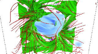
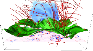
Figure 1.— Three-dimensional snapshot of one of the 3D rMHD models (model H): top view (left panel) and side view (right panel). Some selected magnetic field lines are shown in red to give an indication of the magnetic field topology in the corona. The isosurfaces of Fe xii and Ca xvii emission are shown in green and blue respectively. We also show at the photospheric layer (z=0 Mm) the strength of the vertical magnetic field in blue-red color scale.

Ample efforts have been devoted to the accurate determination of the thermal structuring of coronal plasma to derive robust observational constraints on the coronal heating mechanism(s). The plasma temperature distribution of the quiet corona and of active regions has been investigated through imaging data and spectroscopic observations (e.g., Brosius et al., 1996; Landi & Landini, 1998; Aschwanden et al., 2000; Testa et al., 2002; Del Zanna & Mason, 2003; Reale et al., 2007; Landi et al., 2009; Shestov et al., 2010; Sylwester et al., 2010). Several recent studies have focused on EUV spectra obtained with the Hinode Extreme Ultraviolet Imaging Spectrometer (EIS; Culhane et al. 2007) which provides good temperature diagnostic capability, together with higher spatial resolution and temporal cadence than previously available (e.g., Watanabe et al., 2007; Warren et al., 2008; Patsourakos & Klimchuk, 2009; Brooks et al., 2009; Warren & Brooks, 2009; Testa et al., 2011; Tripathi et al., 2011). Imaging observations obtained by the SDO Atmospheric Imaging Assembly (AIA; Lemen et al. 2012) in narrow EUV bands have also been used for studying the plasma temperature distribution, especially in active region loops (e.g., Schmelz et al., 2010; Aschwanden & Boerner, 2011; Aschwanden et al., 2011; Schmelz et al., 2011), also in conjunction with EIS data (e.g., Brooks et al., 2011; Warren et al., 2011; Testa & Reale, 2012).

The optically thin nature of the coronal EUV and X-ray emission implies that the emission observed in the resolution element (instrument pixel) is generally produced by several independent structures along the LOS. Most plasma diagnostics rely on some homogeneity assumptions (e.g., constant plasma density along the LOS) whereas these overlapping structures can in principle have very different plasma parameters. This poses significant challenges for interpreting the meaning of the derived plasma parameters (which are by necessity weighted averages of the distributions along the LOS) in terms of the actual physical conditions of the plasma. Further assumptions typically made for specific diagnostics (e.g., on the functional form and smoothness of the EMD) also have a potentially significant impact on the accuracy of the diagnostics. Several efforts have been carried out to test the accuracy of the plasma temperature diagnostics. For instance, the notorious challenges in determining the emission measure distribution and its confidence limits have been addressed in several studies (e.g., Craig & Brown, 1976; Judge et al., 1997; McIntosh, 2000; Judge, 2010; Landi & Klimchuk, 2010; Landi et al., 2012; Hannah & Kontar, 2012). The main limitation of these previous efforts lies in the necessarily simplified test cases adopted.

In this paper we use advanced 3D radiative MHD simulations of the solar atmosphere with the Bifrost code (Gudiksen et al., 2011) to carry out detailed tests of coronal plasma temperature diagnostics. We focus on the plasma temperature diagnostics using current spectral (Hinode/EIS) and imaging (SDO/AIA) data. We synthesize EIS and AIA data from 3D radiative MHD (rMHD) simulations and analyze them like real data, and use the comparison of the thermal distributions inferred from the synthetic data with the “true” distributions, which in the case of the simulations are known, to carefully assess the accuracy of the diagnostics. These 3D simulations provide us with the opportunity to improve upon previous work by exploring more realistic configurations, with significant superposition of different structures along the LOS, allowing a statistical approach to determine the accuracy and limitations of the plasma diagnostics, for a variety of spatial and thermal structuring of the plasma. The three dimensional nature of the simulations also allows us to explore a variety of realistic viewing angles, reproducing typical distributions of structuring ranging from on disk to limb observations.

In Section 2 we describe the analysis methods, we include a short description of the Bifrost code, and discuss the characteristics of the 3D rMHD models and of the corresponding synthetic observables used in this work. The analysis of the synthetic data and the results of the determination of the plasma temperature distribution are presented and discussed in Section 3. We summarize our findings and draw our conclusions in Section 4.

2. Analysis Methods

In this work we investigate how accurately the thermal distribution of the plasma can be inferred from coronal observations that are currently available. The observed intensities of a set of spectral emission lines constrain the plasma temperature distribution, as they depend on the abundance $A_{Z}$ of the emitting element, the plasma emissivity of the spectral feature $G_{\lambda}(T,n_{e})$ as a function of temperature $T$ and electron density $n_{e}$, and the differential emission measure distribution $DEM(T)$:

$$I_{\lambda}=A_{Z}\int_{T}G_{\lambda}(T,n_{e})DEM(T)\,dT$$ (1)

where $DEM(T)=n_{e}^{2}\,dV/dT$ $[{\rm cm}^{-3}{\rm K}^{-1}]$. Analogously, in the case of imaging observations in broad/narrow passbands the observed intensity in a channel will depend on the temperature response function, $R_{\rm chan}(T)$:

$$I_{\rm chan}=\int_{T}R_{\rm chan}(T)DEM(T)\,dT.$$ (2)

Throughout the paper, instead of the DEM(T) we will discuss the emission measure distribution $EM(T)$  which is obtained by integrating the differential emission measure distribution $DEM(T)$ in each temperature bin; here we use a temperature grid with constant binning in logarithmic scale ($\Delta\log T=0.05$).

Figure 2.— Histogram of the electron density (left panel) and temperature (right panel) for the two used snapshots (for the voxels with $\log T\geq 5.3$). The simulation “C” modeling the smaller region with emerging flux (solid line) is characterized by lower coronal temperature than the larger simulation “H” (dashed lines), and it has a broader distribution of densities (where the tail at $\log n_{e}\gtrsim 10$ corresponds to dense plasma in the emerging flux region).

Several methods have been developed to reconstruct emission measure distributions from a set of observed intensities in lines, or passbands in the case of imaging observations (see e.g., review by Phillips et al. 2008, and the discussion and references in Hannah & Kontar 2012). Here we test the Monte Carlo Markov chain (MCMC, hereafter) forward modeling method (Kashyap & Drake, 1998), which is widely used and considered to provide robust results (see e.g., Landi et al. 2012; Hannah & Kontar 2012; see also http://www.lmsal.com/$\sim$boerner/demtest/ for a recent comparative analysis of results from different methods, applied to AIA). With respect to several other methods, the MCMC method has the advantages of not imposing a pre-determined functional form for the solution, and, most importantly, of estimating the uncertainties associated with the resulting emission measure distribution (see e.g., Kashyap & Drake, 1998; Testa et al., 2011, for additional details). We use the Package for Interactive Analysis of Line Emission (PINTofALE, Kashyap & Drake 2000) which is available as part of SolarSoft. Though no pre-determined functional form is imposed, the MCMC method does apply some smoothness criteria which are locally variable and based on the properties of the temperature responses/emissivities for the used data, instead of being arbitrarily determined a priori.

Table 1EIS lines synthesized from 3D models and used for reconstructing the emission measure distribution.

$\lambda$[Å]	Ion	$\log(T_{\rm max}[{\rm K}])$	Notes
268.991	Mg vi	5.65	sb
185.213	Fe viii	5.70
278.404	Mg vii	5.80
275.361	Si vii	5.80
188.497	Fe ix	5.90
184.537	Fe x	6.05
188.216	Fe xi	6.15
195.119	Fe xii	6.20	sb
274.204	Fe xiv	6.30
284.163	Fe xv	6.35
262.976	Fe xvi	6.45
208.604	Ca xvi	6.70
192.853	Ca xvii	6.75	bl
254.347	Fe xvii	6.75

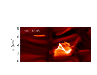
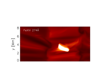
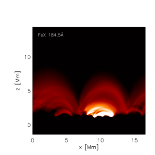
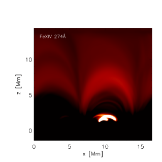
Figure 3.— Synthetic top-view (top row) and side-view (bottom row) Fe x (184.5Å) and Fe xiv (274.2Å) images from the small cooler snapshot, at the intrinsic resolution of the simulation.

For a given simulation snapshot, which provides the electron density $n_{\rm e}$ and temperature values for each grid point (voxel) in a three dimensional box (see section 2.1 for a description of the characteristics of the simulations we analyzed), and a selected LOS we proceed as follows:

• Using the $n_{\rm e}$ and T values, and the emissivities from CHIANTI (Dere et al., 1997, 2009) we synthesize intensities of a set of EIS lines and in the 6 AIA coronal channels, using the optically thin approximation and statistical ionization equilibrium;

• by integrating through the box along the LOS, and degrading the spatial resolution to the instrument resolution, we obtain synthetic coronal images in the different lines/passbands;

• we consider two cases: with or without photon (Poisson) noise; i.e., in the latter case we randomize the intensities according to the photon counting statistics. The noise level and the uncertainties associated with the intensities are calculated by assuming signal-to-noise ratios typical of actual observations;

• we use the intensities and uncertainties, in each pixel, as input for the MCMC routine to calculate the $EM(T)$ solution, pixel by pixel;

• we analyze the results, using several parameters to assess the ability of the method to reproduce the input intensities and the “true” $EM(T)$, which in these test cases are known.

In the following subsection, section 2.1, we describe in detail the choices and assumptions made, and the characteristics of the selected simulations and of the resulting synthetic data.

2.1. 3D Models and Synthetic Observables

The model considered spans from the upper layer of the convection zone up to the low corona, and self-consistently produces a chromosphere and hot corona, through Joule dissipation of electrical currents. In order to investigate the robustness of the $EM(T)$ reconstruction method for a wide range of plasma conditions, we selected snapshots from two simulations that are characterized by significantly different parameters (strength and spatial distribution of the seed magnetic field, and dimensions of the box), which leads to significantly different distributions of temperature and density throughout the box.

We analyze one of the snapshots from the simulation that was previously used to investigate the relative contribution of different lines to the emission in the AIA passbands (Martínez-Sykora et al., 2011). This simulation covers a volume ($x,y,z$, where $z$ is the vertical direction) of $16\times 8\times 16$ Mm³ ($512\times 256\times 365$ grid points; with $\Delta x=\Delta y\sim 32$km, and $\Delta z$ non-uniform and smaller where gradients are large with values $\Delta z\approx 28$km up to a height of 4Mm and increasing to $\approx 150$km at the top of the computational box), and is highly dynamic yielding coronal temperatures that increase with time. We used an intermediate snapshot ($t=1200$s), where the distribution of temperature peaks around $\log(T[K])\sim 6.25$, and $\log T_{\rm max}\sim 6.4$. As we discussed in Martínez-Sykora et al. (2011), the plasma conditions of this simulation represent a good comparison for quiet Sun/coronal hole conditions, with some small emerging flux regions, e.g., small bright points. In the following we use the label C to refer to this cooler and smaller snapshot.

The other snapshot we consider (H, hereafter), is from a simulation modeling a larger region ($24\times 24\times 16$ Mm³; $768\times 768\times 768$ grid points; $\Delta x=\Delta y\sim 31$km, $\Delta z\approx 14$km up to a height of 4Mm and increasing to $\approx 80$km at the top of the computational box; see Figure 1), with a magnetic field configuration consisting of two small regions of opposite polarities similar to a small active region (Carlsson et al., in preparation). The distribution of coronal temperatures is also similar to typical active region values, with a peak around $\log(T[K])\sim 6.6$, and $\log T_{\rm max}\sim 6.7$.

Figure 2 shows the distributions of electron density and temperature throughout the simulation box, for the two selected snapshots, including only plasma with $\log T$ higher than 5.3. These distributions show that simulation “C”, modeling the smaller region with emerging flux, is characterized by lower coronal temperature than the larger simulation “H”, and it has a broader distribution of densities.

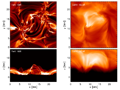
Figure 4.— Synthetic top-view (top row) and side-view (bottom row) Fe xii (195.1Å) and Ca xvii (192.8Å) images, at the intrinsic resolution of the simulation, from the larger and hotter snapshot (H) of the numerical simulation containing a plage-like region, representative of the core of a small active region.

Intensities of a selection of EIS lines and AIA passbands were computed for each voxel of the 3D simulation box $V_{xyz}$, using the plasma electron density and temperature values and using the density and temperature dependent contribution functions $G(T,n_{e})$ from CHIANTI (Dere et al., 1997, 2009), assuming coronal abundances (Feldman, 1992), and the ionization fractions of chianti.ioneq. For AIA we compute synthetic intensities in the coronal passbands (94Å, 131Å, 171Å, 193Å, 211Å, 335Å), by calculating the spectra (line by line, taking into account the temperature and density dependence of the contribution function for each line, and adding the continuum emission) and folding them through the effective area of each channel (Boerner et al., 2012). In the case of EIS we selected a set of lines that provide a good coverage of the temperature range $\log T\sim 5.6-6.7$, but using a relatively limited number of lines, representative of a typical EIS observation: we selected 14 lines, which are listed in Table 1.

Images are then derived for each snapshot, and for two different LOS, by integrating the emission through the simulated box along the LOS: along the horizontal direction $y$ for the “side view”, and along the vertical direction $z$ in the case of the “top view”, analogously to the case presented in Martínez-Sykora et al. (2011). Figures 3 and 4 show examples of such images, at the intrinsic resolution of the simulations. In addition, we degrade the spatial resolution to the instrumental spatial resolution: 0.6 arcsec/pixel for the AIA synthetic data, and 1 arcsec/pixel for EIS.

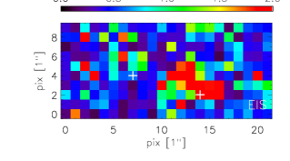
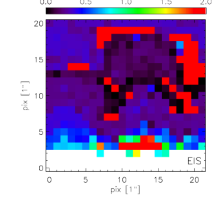
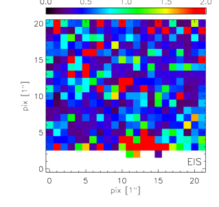
Figure 5.— Maps showing the $\chi^{2}_{0}$ for the EMD derived using the EIS lines listed in Table 1, for snapshot C, for the two LOS, “xy” (top), and “xz” (bottom). The right column shows the case where Poisson noise has been included. The crosses mark two pixels with significantly different $\chi^{2}_{0}$ that will be analyzed in more detail later in the paper (see Figure 8). Pixels where the EMD is not calculated - because less than 5 lines/channels have non-negligible intensity - are plotted in white color.

In order to compute the uncertainties of the simulated intensities we assume a signal-to-noise ratio (S/N) typical of well exposed active region observations (e.g., Reale et al., 2011). For the bright channels of AIA (171Å, 193Å, 211Å) we use the DN pix^-1 assuming typical exposure times in a single image ($t_{\rm exp}\sim 2$s). For the other channels (94Å, 131Å, 335Å) which typically have significantly fainter emission we use the S/N calculated assuming the exposure of 10 summed images (corresponding to $t_{\rm exp}\sim 30$s) . In the case of EIS, we calculate the S/N by scaling the images so that the Fe xii 195Å line, which is usually one of the brightest emission lines in EIS observations, has 500 counts, as in typical observations, and computed the uncertainties from photon counting statistics. We first considered the case without Poisson noise, and then included the Poisson noise by randomizing the intensity values assuming the photon counting statistics of typical AIA and EIS observations as described above.

In appendix A we present a comparison of the synthetic intensities derived from the simulations, as described above, with measured intensities from recent SDO/AIA observations. This comparison shows that the simulations here considered yield emission values of similar order of magnitude of real observations, and therefore provide a sensible test case for the coronal diagnostics.

3. Results

Following the procedure described in detail in section 2, we analyzed the synthetic data to diagnose the plasma temperature distributions, pixel by pixel, using the MCMC reconstruction method. We will first discuss the results obtained using the EIS synthetic data, and then describe the results obtained with the AIA intensities.

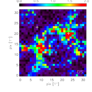
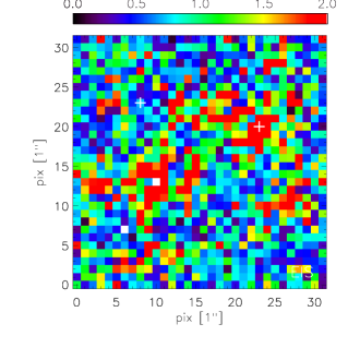
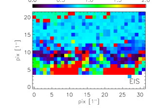
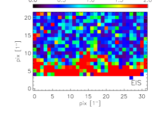
Figure 6.— $\chi^{2}_{0}$ maps analogous to Figure 5 but for snapshot H.

When analyzing real data, the only measure of the goodness of the inferred emission measure distribution consists in the agreement between the measured intensities and the emissions predicted using the best fit EMD. Therefore, as a first step, we show the maps of $\chi^{2}_{0}$ ( $=\Sigma_{j}[(I_{j,pred}-I_{j,obs})/\sigma_{j}]^{2}/df$, where $I_{j,obs}$ and $\sigma_{j}$ are the synthetic intensity and associated error for the line/channel j, $I_{j,pred}$ is the intensity predicted by the best fit EMD and $df$ are the degrees of freedom), for both snapshots and both LOS, using the EIS synthetic intensities (snapshots C and H in Figure 5, and 6, respectively). We show both the case without Poisson noise (left), and including Poisson noise (right). In both cases the errors on the intensities, $\sigma_{j}$, are calculated as the Poisson error on the counts values. For both snapshots the $\chi^{2}_{0}$ maps indicate that the inferred EMD on average reproduce the “measured” fluxes adequately. The case without noise is characterized by $\chi^{2}_{0}$ lower than 1 over large areas, while areas with large $\chi^{2}_{0}$ present clear structuring, which is still present in the case including the effect of noise.

For the top view case, the poorer results in those areas appear to be related to the plasma electron density. To investigate this effect, we use the diagnostic based on the Fe xii line ratio 186.88Å/195.12Å, which is one of the most useful density diagnostics accessible with EIS spectra (e.g., Young et al., 2009), and included in many EIS observing programs.

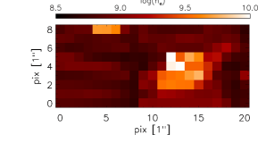
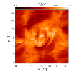
Figure 7.— Maps of electron density derived from synthetic data for the two snapshots (C, top, H, bottom), for the top view, using the Fe xii diagnostics (186Å/195Å) available with EIS observations (see e.g., Young et al. 2009).

In Figure 7 we show the top view map of electron density obtained from the ratio of the synthetic Fe xii intensities, computed from the two snapshots. By comparing these density maps to the $\chi^{2}_{0}$ plots (top row, Figures 5 and 6), it is clear that the high density regions, such as for instance the emerging flux region of snapshot C or footpoint (“moss”) regions of snapshot H, generally correspond to high $\chi^{2}_{0}$ areas.

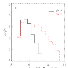
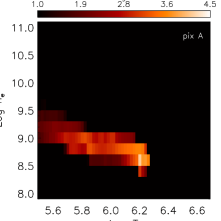
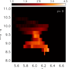
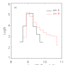
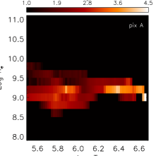
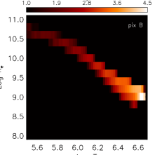
Figure 8.— Distribution of electron density, from the simulations, in the voxels contributing to two pixels with different $\chi^{2}_{0}$ (pixel A with $\chi^{2}_{0}<1$; pixel B with $\chi^{2}_{0}\gtrsim 2$) in the top view for each snapshot (simulation C in the top row and simulation H in the bottom row) to illustrate the effect of the mixing of plasma volumes characterized by significantly different plasma parameters. The selected pixels are marked in the plots showing the $\chi^{2}_{0}$ maps (Figure 5 and  6 for C and H respectively). Histograms of densities in the two pixels are shown in the left panel; 2D histograms, as a function of both temperature and densities are also shown (middle: pixel A; right: pixel B).

As an example, in Figure 8 we show the electron density distribution from the simulations, within two pixels with significantly different $\chi^{2}_{0}$ (with pixel A showing lower $\chi^{2}_{0}$ than B), in the top view case for each of the two snapshots. The selected pixels are marked in Figure 5 and  6 (top row panels). We find that the plasma in pixel B ($\chi^{2}_{0}\gtrsim 2$) has a distribution of density along the LOS much broader than the plasma in pixel A. This leads to a worse determination of the emission measure and worse match of the observed fluxes: even if the selected lines, similar to typical analyses of real data, are mostly insensitive to electron density, their small density dependency significantly affects the diagnostics of emission measure distributions when there is significant mixing of plasmas with different electron densities within the LOS. The same effect of density mixing is causing the large $\chi^{2}_{0}$ regions at the loop footpoints in the side views of both snapshots (bottom panels of Figure 5 and 6).

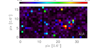
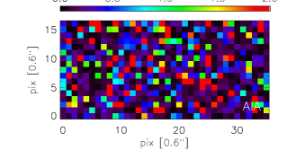
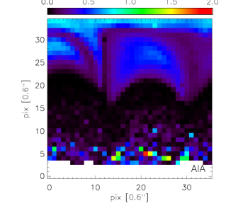
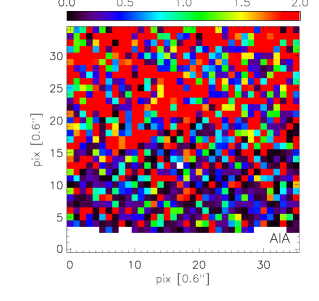
Figure 9.— Maps showing the $\chi^{2}_{0}$ for the reconstruction of the EMD using the AIA intensities, for snapshot C. As in Figure 5, we show the results for the two LOS, “xy” (top), and “xz” (bottom), and also the case including the Poisson noise (right column).

For the side view we note that for snapshot H, in the higher atmosphere, where the temperature distribution in each pixel is essentially isothermal at high temperatures (see also appendix B), the case including the noise tends to have slightly lower $\chi^{2}_{0}$ values (Figure 6). We interpret this effect as due to the extremely narrow (isothermal) distribution: the MCMC method applies some physically based, locally variable, smoothness criteria based on the properties of the temperature responses/emissivities for the used data (see also discussion in Kashyap & Drake 1998; Testa et al. 2011), and therefore it does not perfectly recover purely isothermal distributions; the effect of the noise mimics slight departures from isothermal distributions and therefore the MCMC methods finds better matches to the intensities. A similar effect is also observed for small regions of snapshot C (e.g., the high $\chi^{2}_{0}$ strip at z=19 pix and x from pixel 7 to 14).

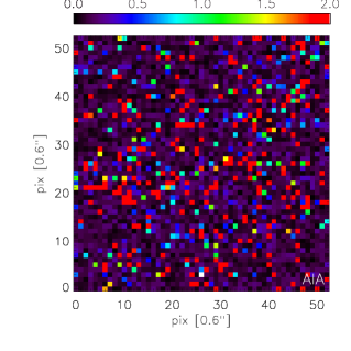
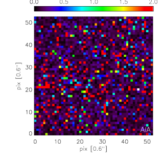
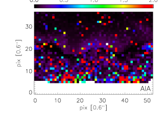
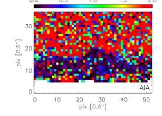
Figure 10.— $\chi^{2}_{0}$ maps analogous to Figure 9, for snapshot H.

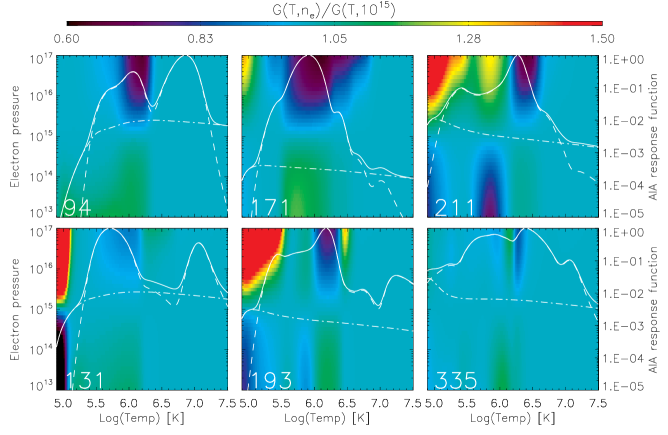
Figure 11.— Dependence of AIA temperature responses on plasma pressure ($n_{e}\times T$ [cm^-3 K]). In the pressure-temperature space, we plot maps of the ratio of the AIA response to the response calculated for a pressure of $10^{15}$ cm^-3 K, which is the pressure assumed for the standard AIA temperature responses available in SolarSoft. From left to right: top - 94Å, 131Å, 171Å; bottom - 193Å, 211Å, 335Å passbands. We overplot the default AIA temperature responses (white lines; in units of $[$DN$~{}s^{-1}$ pix^-1 cm${}^{5}]$, and normalized to their peak), also showing the contribution of the lines (dashed lines) and the continuum emission (dot-dashed lines).

We now consider the $\chi^{2}_{0}$ maps obtained for the analysis of the AIA synthetic intensities; Figures 9 and 10 show the maps for snapshot C and H respectively (analogous to the EIS results of Figures 5, and 6). For snapshot C the top view shows a few pixels with higher $\chi^{2}_{0}$ in the region corresponding to the dense emerging flux region, similarly to the EIS case. For snapshot H there is no clear correspondence between the $\chi^{2}_{0}$ value and the regions with high density mixing. This can be explained by looking at the density sensitivity of the AIA bands, which we have already discussed in Martínez-Sykora et al. (2011) and summarize in Figure 11. The plots in Figure 11 show that most channels have limited density sensitivity, which becomes negligible at high temperature. Therefore we expect less of a density effect for snapshot H where high temperature plasma ($\log T>6.5$; see also appendix B) largely contributes to the observed intensities. In the side view case, the intensities are reproduced quite well in the cases that do not include Poisson noise, whereas the cases including noise show large areas of high $\chi^{2}_{0}$ values, especially at large heights. The larger effect of the noise for AIA is due to the fact that for the side view, the AIA intensities are rather low (see also Figure 26) in some channels, especially in 131Å for both snapshots and 94Å for snapshot C. These channels are more sensitive to the cool plasma (though, for snapshot H the 94Å intensity is largely due to the Fe xviii emission from the high temperature plasma) which has very small or zero contribution higher up in the atmosphere, where the plasma is close to isothermal (as we will show in detail in section 3.1). The low statistics in few channels makes the fit sensitive to the noise. As a result, the fits become worse when including the effect of Poisson noise. We have investigated the results for significantly larger S/N ratio for side view case of snapshot H. We re-run the case including noise, but assuming exposure times that correspond to 50 images for all AIA channels. We find that for very large S/N values the $\chi^{2}_{0}$ values for the intensities tend to get large, because of the very small errors associated with the intensities (down to the level of $\sim 0.1\%$ for the brightest channels). We find that in order to get reasonable $\chi^{2}_{0}$ values the MCMC procedure needs to be run with a significantly larger number of simulations to reproduce the intensities to that level of accuracy. However, as we will discuss later in section 3.2, results show that the effect of the noise is not the main factor that determines the ability of the MCMC method to reconstruct EMDs from AIA data.

For snapshot H, for both LOS, for the case without noise the $\chi^{2}_{0}$ values are generally worse than the corresponding C snapshot (Figure 10). We interpret this as an effect of the broader temperature distributions (especially in the top view) extending to rather high temperatures ($\log T[K]\gtrsim 6.6$; see also following Figures 16 and 17, and appendix B and section 3.1). In this temperature regime AIA provides less reliable temperature diagnostics than at lower temperatures ($\log T[K]\sim 6-6.3$) where several AIA channels have high sensitivity and their relative shapes in temperature response provide better constraints to the plasma temperature distributions.

We note that the uncertainties we assume here are generally significantly smaller than the errors typically associated to intensity measurements in real data for the EMD reconstruction. Those errors are typically larger than the uncertainties associated with photon counting statistics because they also take into account uncertainties in atomic data which are difficult to quantify. In the test presented in this paper, there are no uncertainties to be associated with the atomic data, since we use the same atomic data to synthesize the intensities and to infer from them the EMD. Nevertheless, the small errors we assume can in part explain the sometimes large values of $\chi^{2}_{0}$ we obtained here.

The results discussed so far provide us with a measure of how well the temperature distributions inferred using the MCMC method are able to reproduce the “measured” intensities. We now discuss in detail the comparison of the derived EMD with the true emission measure distributions. We looked at different parameters to assess the robustness and limits of the reconstruction method in recovering the plasma temperature distributions: (1) the temperature at which the EMD peaks ($T(EMD_{max})$) within the temperature range $\log T[K]=[5.5-6.7]$, (2) the EM values integrated in broad temperature bins, and (3) the full EMD (i.e., at the fine temperature resolution). The temperature of the EMD peak is not necessarily a good indicator to evaluate the goodness of the MCMC solution, especially for broader and more structured EMDs. We therefore present the analysis of $T(EMD_{max})$ in appendix A, summarizing here only the main results, while in the main text we will focus on the other two comparisons (sections 3.1 and 3.2).

The results presented in appendix A show that the MCMC method performs well in recovering the $T(EMD_{max})$ when the EMD is close to isothermal. For broad EMDs the method tends to generally underestimate $T(EMD_{max})$, due to several factors, including poor constraints beyond the $\log T[K]=[5.5-6.7]$ range, and limited capability of the method to recover sharp features.

3.1. Emission measure maps

One of the approaches we use to determine the accuracy of the EMD diagnostics is by looking at the maps of emission measure in different temperature ranges.

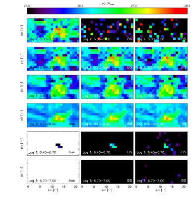
Figure 12.— Emission measure maps for the top view of snapshot C, from the model (left panels) and from EIS synthetic data (without noise or including noise, in the middle and right panels respectively), integrated in six temperature bins: $\log T[K]:$ 5.0-5.5, 5.5-5.8, 5.8-6.1, 6.1-6.4, 6.4-6.7, 6.7-7. White corresponds to values of EM equal to zero.

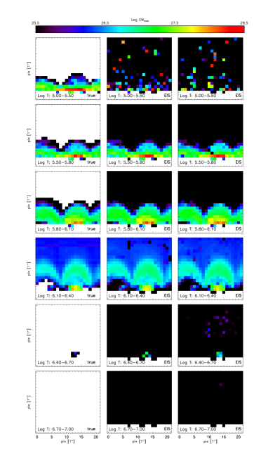
Figure 13.— Comparison of emission measure maps obtained from the analysis of EIS synthetic data of snapshot C, analogous to Figure 12 but for the side view.

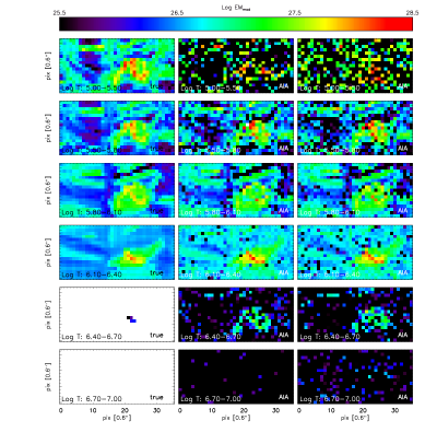
Figure 14.— Comparison of emission measure maps obtained from the analysis of the top view AIA synthetic data of snapshot C, analogous to Figure 12.

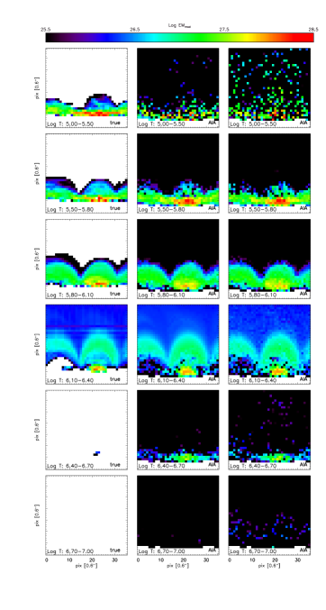
Figure 15.— Comparison of emission measure maps obtained from the analysis of the side view AIA synthetic data of snapshot C, analogous to Figure 12.

In Figure 12 and 13 we show, for top and side view of snapshot C respectively, the maps of the true emission measure (left column), in six relatively broad temperature bins, spanning the temperature range $\log T[K]=5-7$. Figures 16 and 17 show the analogous plots for snapshot H. Figures 14 and 15 (for snapshot C), and Figures 18 and 19 (for snapshot H) also show the EM maps derived at the AIA spatial resolution, for direct comparison with the corresponding maps derived by the analysis of the synthetic data. These plots show, for the top view, how the plasma is characterized by rather broad temperature distributions in most locations, especially in locations associated with the emerging flux region for snapshot C, and with the loop footpoints (“moss”) for snapshot H (see Figures 3 and 4). The simulated corona in snapshot C lacks significant plasma volumes at temperatures above $\log T[K]=6.4$, while for snapshot H the coronal plasma reaches temperature even higher than $\log T[K]=6.7$ in a hot loop-like feature, which emits brightly in e.g., Ca xvii (Figure 4). The side view shows loop-like features in the lower corona of both snapshots, with rather broad temperature distribution. Higher up in the corona the plasma is characterized by narrow temperature distributions peaking around $\log T[K]\sim 6.2$ in snapshot C, and $\log T[K]\sim 6.6$ in snapshot H.

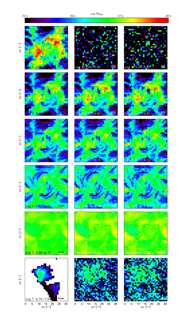
Figure 16.— Emission measure maps for the top view of snapshot H, from the model (left panels) and from EIS synthetic data (without noise or including noise, in the middle and right panels respectively), integrated in six temperature bins: $\log T[K]:$ 5.0-5.5, 5.5-5.8, 5.8-6.1, 6.1-6.4, 6.4-6.7, 6.7-7. Figure analogous to Figure 12, but for snapshot H.

Figure 17.— Comparison of emission measure maps obtained from the analysis of the side view EIS synthetic data of snapshot H, analogous to Figure 16.

The corresponding maps for the EMD derived from the analysis of EIS and AIA synthetic data are shown next to the true maps for all the cases, without or including noise (in center and right column respectively of Figures 12-15, and 16-19).

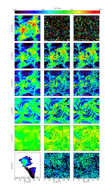
Figure 18.— Comparison of emission measure maps obtained from the analysis of the top view AIA synthetic data of snapshot H, analogous to Figure 16.

For EIS, the general features of the emission measure distribution in the central temperature bins (i.e., between $\log T[K]\sim 5.5$ and $\sim 6.4$ for snapshot C and in the range $\log T[K]\sim 5.5$-$6.7$ for snapshot H), are recovered quite well, also when including the effect of the noise. In the top view case, for both snapshots, in the temperature bin at the low end of the constrained range ($\log T[K]\sim 5.5-5.8$) the EM are overestimated in several pixels because of the same effects discussed in appendix B, because of the lack of constraints at lower temperatures. The noisy results at the low and high temperature end are expected considering the poor constraints provided by the selected EIS lines at those temperatures.

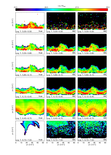
Figure 19.— Comparison of emission measure maps obtained from the analysis of the side view AIA synthetic data of snapshot H, analogous to Figure 16.

With AIA, though some structures such as the side view loops are still apparent in the reconstructed EM maps to a lesser extent, the EM maps derived from the analysis of the synthetic data are not reproducing the true maps very accurately, especially for the top view case. For instance for the top view case of snapshot C (14) the maps derived from AIA present significant EM, especially in the emerging flux region, in the bin temperature $\log T[K]\sim 6.4-6.7$, where the real EM is zero almost everywhere.

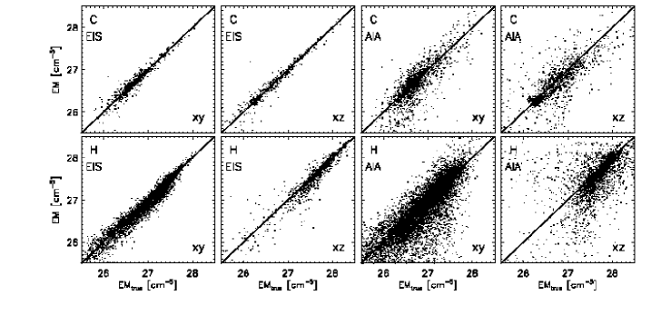
Figure 20.— Scatter plots of EM derived from EIS (first two columns) and AIA (right columns) synthetic data from the two snapshots (cool simulation “C” in the top row, and hot simulation “H” in the bottom row), vs. the corresponding true EM values. For each of the panels, we plot the values for the central four temperature bins ($\log T[K]:$ [5.5-5.8],[5.8-6.1],[6.1-6.4],[6.4-6.7]), and excluded the EM values for the two temperature bins at the extremes of the range ($\log T[K]:$ [5.0-5.5],[6.7-7.0]).

In Figure 20 we show, for all the cases including the effect of the noise, the scatter plots of the derived vs. true EM, for the central four temperature bins, i.e., $\log T[K]:$ 5.5-5.8, 5.8-6.1, 6.1-6.4, 6.4-6.7. These plots show that, when integrating in broad temperature ranges ($\Delta\log T=0.3$), the EM derived from EIS reproduce rather well the true EM, while the EM derived from AIA have significantly larger scatter for the whole range of EM values. We note that these bins are significantly wider than typically used by observers when deriving EMDs.

3.2. Full emission measure distributions

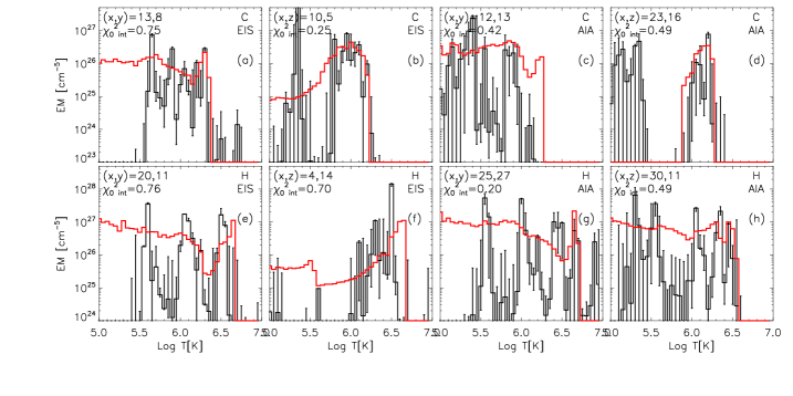
Figure 21.— Sample of comparisons of true (red curves) and derived EMD (including noise), for one pixel for each case. The results from EIS synthetic data are shown in the left two columns, and the ones from AIA in the right two columns. The results for snapshot C are shown in the top row, while the bottom four panels show the results for snapshot H.

In the previous section we have addressed a comparison of the general properties of the EMDs derived from synthetic EIS and AIA data with the input emission measure distributions from 3D rMHD simulations. In this section we will assess how well the derived EMDs reproduce the true EMDs in their details, on the finest temperature scale, and explore to what level of detail the MCMC EMD reconstruction method is reliable.

In Figure 29 we have already shown the full EMDs for a selection of pixels chosen to explain the systematic discrepancies in $T(EMD_{max})$. That set of plots already shows that, while as discussed above some general features of the EMD are recovered by the MCMC method, when comparing the EMDs on the fine temperature scale (i.e., here we used $\Delta\log T[K]=0.05$ which is the typical intrinsic resolution of atomic data, and also the typical resolution used by observers), the derived EMD can significantly depart from the true distributions.

In Figure 21 we show the comparison of the true and derived EMD for a pixel selected for each case (for every snapshot and LOS, for the cases including noise), to show examples where, even if the intensities are reproduced within the errors ($\chi^{2}\lesssim 1$), the derived and true EMD present significant discrepancies.

First we note that in most of the examples of Figures 29 and  21, there are several temperature bins within the $\log T=[5.5-6.7]$ range where the true EMD is not compatible with the derived EMD within the uncertainties. In general we find that the EMDs resulting from the analysis of EIS synthetic data reproduce the general properties of the EMDs - such as bulk of the emission and general shape - significantly better than the corresponding AIA EMDs, as also shown in the previous section 3.1. However, even in the temperature range $\log T[K]\sim[5.5-6.7]$ where the emission measure distribution should be well constrained by the selected spectral lines, the best fit EMD can be very noisy and present peaks and valleys which are not present in the true EMD.

We note that, as discussed by Kashyap & Drake (1998) and Testa et al. (2011), the uncertainties associated with the EMD solution are correlated in the different temperature bins, and therefore, what are shown as error bars in the single temperature bins cannot strictly be interpreted as error bars for the EMD value in that bin, and instead they describe the range containing 68% of the sets of solutions. Nevertheless, since they are typically used as error bars we investigate here also the limitations of this assumption.

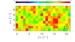
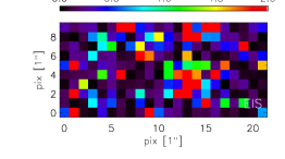
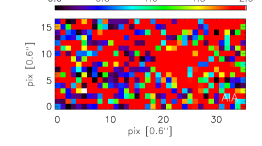
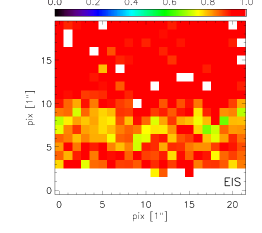
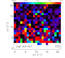
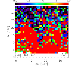
Figure 22.— Left: Maps of the “goodness of fit” for the EMD for the EIS case both top view (top row) and side view (bottom row) for snapshot C. The value in each pixel represents the average over all temperature bins between $\log T=5.5$ and 6.7, of the fraction of the solutions falling in the range between the best fit EMD and the true EMD which is used as a measure of the probability that the true EMD is part of the same distribution of the EMD solutions. A value close to 1 implies that for most temperature bins the true EMD is far from the bulk of the distribution. We use the full temperature resolution ($\Delta\log T[K]=0.05$). Middle: Maps of $\chi^{2}(EMD)$ (see text for definition), parametrizing the ability of the MCMC method to recover the full EMD in each temperature bin from EIS data (including noise). We used $\Delta\log T[K]=0.2$. Right: Maps of $\chi^{2}(EMD)$ for the EMD derived from AIA data (including noise), and assuming $\Delta\log T[K]=0.3$.

In order to assess the ability of the MCMC method to recover the full EMD for all the different cases studied, we use two different ways to parametrize the “goodness of the fit”. First, we use the full information of the set of EMD solution produced by the MCMC routine for each pixel. For a given pixel, and a given temperature bin (we use here the full temperature resolution, i.e., $\Delta\log T[K]=0.05$), we can calculate the fraction of solutions included in the range between the true EMD value and the best fit value. This can be interpreted as a probability for the EMD value to be part of the distribution of Monte Carlo solutions. Since it is not trivial to combine the results of the different temperature bins, we compute an average of these fraction over all temperature bins between $\log T=5.5$ and 6.7. If the average is close to 1, this implies that for most temperature bins the true EMD is far from the bulk of the distribution. We show the maps of the values obtained from the EIS EMDs in this fashion in the left panels of Figure 22 (for snapshot C) and 23 (for snapshot H). The corresponding maps for the AIA EMDs are not shown but are qualitatively very similar to the EIS cases shown here. For the top view cases the maps present similar structuring to the $\chi^{2}_{0}$ maps shown in Figures 5 and 6, with the worst match of EMD found in the regions with large superpositions of plasma structures with different densities and temperatures. For the side view, while lower in the atmosphere the values are similar to the top view case, they become $\sim 1$ everywhere at larger heights. The reason for this is that at larger heights the true EMD are close to isothermal, dropping to zero everywhere outside the peak region. For all the temperature bins where the true EMD is zero, the derived EMDs are non-zero causing large discrepancies in most of the temperature bins.

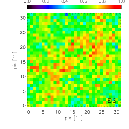
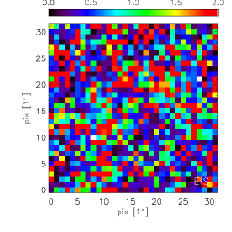
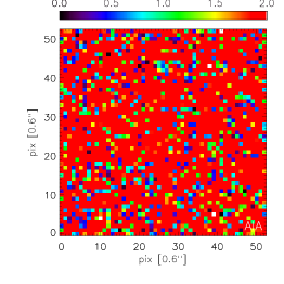
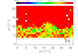
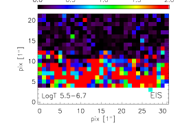
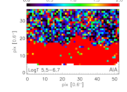
Figure 23.— Plots analogous to plots in Figure 22 but for snapshot H.

Another way to calculate a measure of how well the derived EMDs match the true EMDs is to calculate a $\chi^{2}_{0}(EMD)$ for the EMD, which we define as $=\Sigma_{j}[(EMD_{j,MCMC}-EMD_{j,true})/\sigma(EMD)_{j}]^{2}/df$, where $EMD_{j,true}$ and $EMD_{j,MCMC}$ are respectively the values of the true and derived EMD for the temperature bin $j$, $\sigma(EMD)_{j}$ is the uncertainty of the EMD in the T bin $j$ defined by the range including 68% of the solutions, as described above, and $df$ are the degrees of freedom (as defined at the beginning of section 3). We find that when calculating the so defined $\chi^{2}_{0}(EMD)$ using the fine temperature grid ($\Delta\log T=0.05$) the $\chi^{2}_{0}(EMD)$ values are very large ($\gg 10$) for both the EIS and AIA cases. Therefore we decrease the temperature resolution until the $\chi^{2}_{0}(EMD)$ values become on average more reasonable. We find that this threshold is $\Delta\log T\sim 0.2$ for EIS, and we show the corresponding maps of $\chi^{2}_{0}(EMD)$ in the middle panels of Figure 22 and 23. These maps show the usual pattern of the features with large superposition of different structures, where the agreement is worse, but for the other regions the integration over large temperature bins yields a better match of the derived and true EMDs, by smoothing out the large variability on small temperature scale shown in Figures 29 and  21. We note that for the side view cases, high in the corona, the uncertainties of these EMD on the coarser temperature grid appear even overestimated, since the $\chi^{2}_{0}(EMD)$ drops to very low values. This is consistent with the findings of Landi et al. (2012) who explored the ability of the MCMC methods to diagnose isothermal EMD. Landi et al. (2012) find indeed that for isothermal plasma a bin width of $\Delta\log T\sim 0.05$ is sufficient to diagnose the temperature distribution from spectral data. For AIA, even with $\Delta\log T\sim 0.3$ the $\chi^{2}_{0}(EMD)$ values (maps are shown in the right panels of Figure 22 and 23) are large for the top view cases, in agreement with the results discussed in above section 3.1. The side view cases show that with AIA the temperature binsize $\Delta\log T\sim 0.3$ is adequate to diagnose isothermal plasmas, as shown by the low $\chi^{2}_{0}(EMD)$ values at high $z$ values, but is still insufficient to guarantee a good match of the true EMD where the distributions are significantly multi-thermal. The EMDs derived AIA are a much less accurate reproduction of the true EMDs compared to EIS. This points to a significant problem in relying on AIA data exclusively, to diagnose the plasma temperature distribution. This can be explained by considering two main factors: (1) the smaller number of constraints - AIA data provide a considerably more limited number of constraints (at best 6) compared to EIS; (2) imaging data have significantly more limited temperature diagnostics than spectral data, because of their broader temperature sensitivity (even for the narrow AIA passbands) compared to the resolved spectral lines. In this respect, though outside the scope of this paper, we note that narrow band coronal imagers also have the additional disadvantage with respect to broad band instruments of being critically sensitive to the uncertainties in the atomic data (see, e.g., Testa et al., 2012). We note that the EMDs derived from AIA present significant discrepancies with the true EMDs even in the case that does not include noise, or in the test case with very high S/N discussed at the beginning of this section when we discussed the fit to the observed intensities. We therefore conclude that the limitations in diagnosing EMDs with AIA data are mainly due to the intrinsic characteristics of the (broad) AIA temperature responses, and that the noise is not the main cause of the discrepancies between true and derived EMDs.

While our results imply that in general the MCMC method does not reproduce the true EMDs at the highest temperature resolution, it is preferable for several reasons to run the method at high resolution ($\Delta\log T\sim 0.05$) and then rebin the solution a posteriori. As discussed above (and shown in Figure 22 and 23), the high resolution allows one to find nearly isothermal solutions. Also, we have run for a few pixels the MCMC on the EIS synthetic data using different values of $\Delta\log T$ and found that adopting a too large bin size leads to less stable solutions, due to the rebinning of the temperature response function and consequent loss of temperature information. For instance if the temperature bins become significantly large compared to the peaks in the temperature response functions the rebinned responses often end up with peaks which are much less prominent, and significantly displaced in temperature.

4. Discussion and conclusions

We have presented the results of a test of the limitations of plasma temperature diagnostics that are currently available from spectral and imaging observations of the solar corona. Determining the plasma emission measure distribution is fraught with difficulties, both because of the intrinsic nature of the mathematical inversion problem, which is ill-posed, and because of the limitations of the available data. While imaging instruments provide only moderate temperature diagnostics (compared with spectrographs that can resolve spectral lines), they typically provide significantly better spatial coverage and resolution, and temporal cadence.

Here we used advanced 3D radiative MHD simulations of the solar atmosphere (Hansteen et al., 2007; Gudiksen et al., 2011) as realistic test cases, from which we produced synthetic observables, and applied a Monte Carlo Markov chain forward modeling technique to derive the emission measure distributions (EMD). We then compared the results of EMD reconstruction from imaging (AIA) and spectral (EIS) synthetic data (based on the coronal properties in the models) with the input “true” EMD to establish the limitations of the temperature diagnostic power of the available instruments, and how these results depend on the characteristics of the underlying thermal distributions. We also investigated the effect of the photon counting noise, by running the analysis with or without randomization accounting for Poisson noise.

These 3D simulations provide us with the opportunity to improve upon previous work by exploring more realistic configurations, with significant superposition of different structures along the LOS, allowing a statistical approach to determine the accuracy and limitations of the plasma diagnostics, for a variety of spatial and thermal structuring of the plasma. The three dimensional nature of the simulations also allows us to explore a variety of realistic viewing angles, reproducing typical distributions of structuring ranging from on disk to limb observations.

We assess the robustness of the EMD reconstruction method by using several parameters. We explored the ability of the method in: (a) reproducing the “measured” intensities; (b) determining the temperature of the peak of the emission measure distribution; (c) deriving the emission measure values in broad temperature bins; (d) reproducing the true emission distribution in its details.

The analysis of the spectral EIS synthetic data show that the measured intensities are reproduced generally well by the inferred EMD, even when including the effect of noise, with the exception of regions with mixing of regions with significantly different densities along the LOS. The temperature of the peak of the EMD is reproduced reasonably well for the side view, in larger areas where the EMD is close to isothermal. For the top view, where the EMD are broad and in particular where there are large amounts of dense material and large superposition of different structures (emerging flux region, moss), the temperature of the peak EMD appears to be systematically underestimated. The maps of emission measure, when integrated in broad temperature bins, are similar to the true distributions, in the well constrained range ($\log(T[K])\sim[5.6-6.4]$); the low and high temperature ends of the considered range are rather noisy and present spurious components. However, when considering the direct comparison of the derived EMD curves with the true distributions, at the full temperature resolution, we find that the detailed properties of the true EMD on the smallest temperature scale are not accurately reproduced. The best fit EMD can present peaks which are not displayed by the true EMD, or vice versa, narrow peaks might be missed by the reconstruction method. The worst cases show how the uncertainties do not generally account for these discrepancies, and are therefore likely underestimated by the method. We explore the temperature resolution at which the discrepancies between true and derived EMD become smaller, and we find that for EIS the $\Delta\log T$ needs to be $\gtrsim 0.2$. We therefore conclude that the temperature diagnostic provided by spectral data with enough observational constrains and good temperature coverage, are on average reliable to derive the general characteristics of the emission measure distribution, such as the emission measure in broad temperature bins, but that the results are not robust enough as far as the fine details of the EMD, such as the presence of narrow peaks, are concerned, and that features on scales below $\gtrsim 0.2$ in $\log T$ cannot be trusted.

The results obtained from the analysis of the AIA synthetic data are more unsatisfactory. The synthetic intensities for the side view LOS are low in some channels, making the results more sensitive to the effect of the noise. The maps of temperature at which the EMDs peak show that, as for the EIS case, the temperatures are not very well reproduced, and appear systematically underestimated, especially in the top view case. Also the maps of emission measure integrated in broad temperature bins are a poor match for the true distributions, especially for the top view case. Finally, the direct comparison of derived and true EMD curves at the full temperature resolution indicates discrepancies well beyond the errors, implying that the EMD are not at all well constrained by the AIA data, often not even in their general characteristics. Even degrading the temperature resolution to $\Delta\log T=0.3$ the derived EMD do not match accurately the true EMD, especially where the temperature distributions are broad. We therefore conclude that the limited number of constraints and the broad temperature sensitivity of the AIA passbands, which often present multiple peaks, critically hamper the capability of diagnosing the plasma temperature distribution on the basis of AIA imaging observations exclusively. The addition of simultaneous Hinode/XRT data, which provide complementary imaging observations in X-ray broadbands, might improve considerably the ability to reconstruct EMDs from AIA data, by providing additional constraints, especially at the high temperature end ($\log T\sim 6.5-7$), where AIA provides limited information. We plan to explore this issue in a follow-up paper. In this paper we have not addressed the use of EIS and AIA together because, as discussed here above and in other papers (see e.g., Warren et al. 2011; Testa et al. 2011), the spectral data, when available, provide much better constraints to the temperature distribution of the plasma, compared with imaging data, and the imaging data provide only limited additional constraints. However, imaging data provide a much better temporal and spatial coverage of the coronal plasma, so we focused on investigating the usefulness of imaging data for thermal diagnostics, when spectral data are not available, as in the large majority of solar observations.

The approach adopted here, using 3D simulations, has provided us with the opportunity to improve upon previous work by exploring more realistic configurations, with significant superposition of different structures along the LOS, allowing a statistical approach to determine the accuracy and limitations of the plasma diagnostics, for a variety of spatial and thermal structuring of the plasma. These results provide a stringent and accurate assessment of the limitations of the temperature diagnostics, indicating the extent of the sensitivity of EMD measurements to the structuring along the LOS, and to characteristics inherent to the instrumentation. However, we emphasize that the exercise we carried out focuses on the use of the MCMC reconstruction method, and therefore it only assesses the robustness of this particular method, which is however largely adopted and trusted for studies of emission measure distributions of solar and stellar coronal plasmas. We note that these results actually present an optimistic view, because they do not account for several effects that further complicate real observations, such as for instance uncertainties in both instrument calibration and atomic data, influence of blends in fitting the spectral data, and distribution of element abundances. Finally, the 3D simulations adopted here model limited coronal volumes, therefore likely underestimating the effects of superposition along the LOS.

Appendix A Comparison of synthetic intensities with actual observations

In this appendix we present a comparison of the synthetic intensities derived from the simulations, as described in section 2.1, with measured intensities from recent SDO/AIA observations. We considered AIA observations taken on 2012 January 6, around 23UT (the 193Å full disk image is shown in Figure 24), and selected a few small regions (100 pixels $\times$ 100 pixels, corresponding to $\sim 60$ arcsec $\times$ 60 arcsec) sampling a variety of coronal features, ranging from quiet Sun to active regions, and including areas both on-disk and above limb.

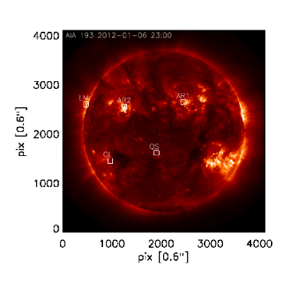
Figure 24.— SDO/AIA 193Å channel full disk observation taken on 2012 January 6 around 23UT, where we selected a subset of small regions ($100\times 100$ pixels) of different coronal features: quiet Sun (QS), cool fan loops (CL), limb (LM), and active region plasma (AR1, AR2). In Figure 25 we show the distributions of the 6 AIA EUV coronal channels intensities for these selected regions, to be compared with the distributions of the synthetic intensities derived from the simulations (shown in Figure 26).

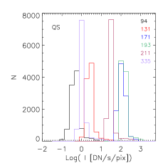
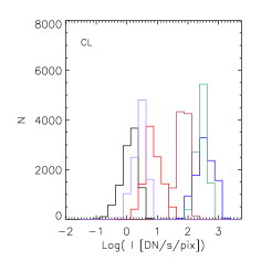
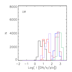
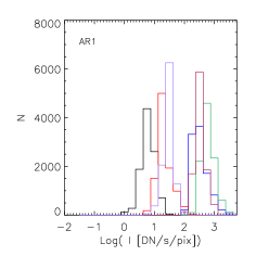
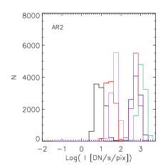
Figure 25.— Histograms showing the distributions of the observed intensities (in DN s^-1 pix^-1) in the AIA channels (shown in different colors, as labeled in the top left panel, QS), for the regions indicated in Figure 24: quiet Sun (QS), cool fan loops (CL), limb (LM), and active region plasma (AR1, AR2).

In Figure 25 we show the distribution of the observed intensities (in units of DN s^-1 pix^-1) in the six selected AIA EUV bands, for the different regions shown and labeled in Figure 24. These plots clearly show that: (a) average absolute intensities change by more than an order of magnitude from region to region; (b) the distribution in each channel, in each of the regions is rather narrow; (c) the distributions of intensities in the 94Å, 131Å, and 335Å channels typically peak at values about two orders of magnitude lower than the intensities in the other three bright channels; (d) the intensities in the 211Å, and 335Å channels typically have relative lower values in cooler regions (quiet Sun and cool fan loops; regions QS and CL).

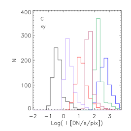
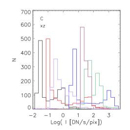
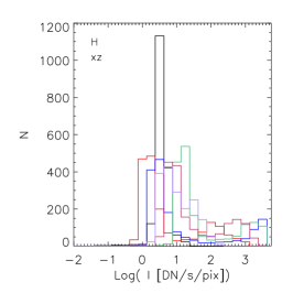
Figure 26.— Histograms showing the distributions of the AIA intensities synthesized from the two snapshots (left panels: smaller cooler snapshot, C; right panels: larger hotter snapshot, H), and for the two different views (“xy” in the top panels and “xz” in the bottom panels).

In Figure 26 we show the distribution of the synthetic intensities in the AIA passbands, for the two lines of sight for each of the two snapshots. The smaller, cooler snapshot (C) is characterized by intensities similar to the values observed in cool fan loops (region CL) and quiet Sun (region QS), whereas the larger and hotter snapshot (H) produces intensities more similar to the observed values of active region plasma (regions AR1 and AR2). We note that, as expected, the top view (“xy”) provides a more realistic comparison for real coronal observations, while for the side view (“xz”) the distributions have tails at low intensity values, which are not observed in the AIA selected data. This is because the small box size does not accurately capture the enormous line-of-sight at the limb in the optically thin corona. However, for the side view of snapshot C the inversion of the peaks of the 335Å and 131Å channels with respect to the top view (i.e., for the side view the 131Å distribution peaks at lower intensity values than the 335Å) reproduces what is observed in actual data at the limb (region LM) compared with quiet on disk regions (QS, CL). We also note that the distributions for snapshot H appear generally broader than the observed distributions. For snapshot C the distribution of each passband peaks around a different value, whereas the observed distributions typically show a common peak for the weaker channels and a separate common peak for the stronger channels. Finally, the intensities in the 94Å channel are systematically lower than the observed values, but this is expected on the basis of recent studies arguing for incompleteness of atomic databases, especially in the 94Å passband (e.g., Testa et al., 2012). By and large, these qualitative comparisons indicate that the simulations produce emission values of similar order of magnitude of real observations, and therefore represent a reasonable test case for the coronal diagnostics.

Appendix B Emission measure peak temperature

See complete preprint version at http://folk.uio.no/bdp/papers/3dEMD_ptesta.pdf

References

- Aschwanden & Boerner (2011) Aschwanden, M. J., & Boerner, P. 2011, ApJ, 732, 81
- Aschwanden et al. (2011) Aschwanden, M. J., Boerner, P., Schrijver, C. J., & Malanushenko, A. 2011, Sol. Phys., 384
- Aschwanden & Nightingale (2005) Aschwanden, M. J., & Nightingale, R. W. 2005, ApJ, 633, 499
- Aschwanden et al. (2000) Aschwanden, M. J., Nightingale, R. W., & Alexander, D. 2000, ApJ, 541, 1059
- Boerner et al. (2012) Boerner, P., Edwards, C., Lemen, J., et al. 2012, Sol. Phys., 275, 41
- Brooks et al. (2009) Brooks, D. H., Warren, H. P., Williams, D. R., & Watanabe, T. 2009, ApJ, 705, 1522
- Brooks et al. (2011) Brooks, D. H., Warren, H. P., & Young, P. R. 2011, ApJ, 730, 85
- Brosius et al. (1996) Brosius, J. W., Davila, J. M., Thomas, R. J., & Monsignori-Fossi, B. C. 1996, ApJS, 106, 143
- Cargill & Klimchuk (2004) Cargill, P. J., & Klimchuk, J. A. 2004, ApJ, 605, 911
- Craig & Brown (1976) Craig, I. J. D., & Brown, J. C. 1976, A&A, 49, 239
- Culhane et al. (2007) Culhane, J. L., Harra, L. K., James, A. M., et al. 2007, Sol. Phys., 243, 19
- Del Zanna (2003) Del Zanna, G. 2003, A&A, 406, L5
- Del Zanna & Mason (2003) Del Zanna, G., & Mason, H. E. 2003, A&A, 406, 1089
- Dere et al. (1997) Dere, K. P., Landi, E., Mason, H. E., Monsignori Fossi, B. C., & Young, P. R. 1997, A&AS, 125, 149
- Dere et al. (2009) Dere, K. P., Landi, E., Young, P. R., Del Zanna, G., Landini, M., & Mason, H. E. 2009, A&A, 498, 915
- Feldman (1992) Feldman, U. 1992, Phys. Scr, 46, 202
- Gudiksen et al. (2011) Gudiksen, B. V., Carlsson, M., Hansteen, V. H., Hayek, W., Leenaarts, J., & Martínez-Sykora, J. 2011, A&A, 531, A154
- Hannah & Kontar (2012) Hannah, I. G., & Kontar, E. P. 2012, A&A, 539, A146
- Hansteen et al. (2007) Hansteen, V. H., Carlsson, M., & Gudiksen, B. 2007, in Astronomical Society of the Pacific Conference Series, Vol. 368, The Physics of Chromospheric Plasmas, ed. P. Heinzel, I. Dorotovič, & R. J. Rutten, 107
- Judge (2010) Judge, P. G. 2010, ApJ, 708, 1238
- Judge et al. (1997) Judge, P. G., Hubeny, V., & Brown, J. C. 1997, ApJ, 475, 275
- Kashyap & Drake (1998) Kashyap, V., & Drake, J. J. 1998, ApJ, 503, 450
- Kashyap & Drake (2000) —. 2000, Bulletin of the Astronomical Society of India, 28, 475
- Klimchuk (2006) Klimchuk, J. A. 2006, Sol. Phys., 234, 41
- Klimchuk & Cargill (2001) Klimchuk, J. A., & Cargill, P. J. 2001, ApJ, 553, 440
- Ko et al. (2009) Ko, Y., Doschek, G. A., Warren, H. P., & Young, P. R. 2009, ApJ, 697, 1956
- Landi et al. (2006) Landi, E., Del Zanna, G., Young, P. R., Dere, K. P., Mason, H. E., & Landini, M. 2006, ApJS, 162, 261
- Landi & Feldman (2008) Landi, E., & Feldman, U. 2008, ApJ, 672, 674
- Landi et al. (2002) Landi, E., Feldman, U., & Dere, K. P. 2002, ApJS, 139, 281
- Landi & Klimchuk (2010) Landi, E., & Klimchuk, J. A. 2010, ApJ, 723, 320
- Landi & Landini (1998) Landi, E., & Landini, M. 1998, A&A, 340, 265
- Landi et al. (2009) Landi, E., Miralles, M. P., Curdt, W., & Hara, H. 2009, ApJ, 695, 221
- Landi et al. (2012) Landi, E., Reale, F., & Testa, P. 2012, A&A, 538, A111
- Lemen et al. (2012) Lemen, J. R., Title, A. M., Akin, D. J., et al. 2012, Sol. Phys., 275, 17
- Martínez-Sykora et al. (2011) Martínez-Sykora, J., De Pontieu, B., Testa, P., & Hansteen, V. 2011, ApJ, 743, 23
- McIntosh (2000) McIntosh, S. W. 2000, ApJ, 533, 1043
- Patsourakos & Klimchuk (2006) Patsourakos, S., & Klimchuk, J. A. 2006, ApJ, 647, 1452
- Patsourakos & Klimchuk (2009) —. 2009, ApJ, 696, 760
- Phillips et al. (2008) Phillips, K. J. H., Feldman, U., & Landi, E. 2008, Ultraviolet and X-ray Spectroscopy of the Solar Atmosphere (Cambridge University Press)
- Reale (2010) Reale, F. 2010, Living Reviews in Solar Physics, 7, 5
- Reale et al. (2011) Reale, F., Guarrasi, M., Testa, P., DeLuca, E. E., Peres, G., & Golub, L. 2011, ApJ, 736, L16
- Reale et al. (2009a) Reale, F., McTiernan, J. M., & Testa, P. 2009a, ApJ, 704, L58
- Reale et al. (2007) Reale, F., Parenti, S., Reeves, K. K., et al. 2007, Science, 318, 1582
- Reale et al. (2009b) Reale, F., Testa, P., Klimchuk, J. A., & Parenti, S. 2009b, ApJ, 698, 756
- Schmelz et al. (2011) Schmelz, J. T., Jenkins, B. S., Worley, B. T., Anderson, D. J., Pathak, S., & Kimble, J. A. 2011, ApJ, 731, 49
- Schmelz et al. (2010) Schmelz, J. T., Kimble, J. A., Jenkins, B. S., Worley, B. T., Anderson, D. J., Pathak, S., & Saar, S. H. 2010, ApJ, 725, L34
- Schmelz et al. (2005) Schmelz, J. T., Nasraoui, K., Roames, J. K., Lippner, L. A., & Garst, J. W. 2005, ApJ, 634, L197
- Schmelz et al. (2009a) Schmelz, J. T., Saar, S. H., DeLuca, E. E., Golub, L., Kashyap, V. L., Weber, M. A., & Klimchuk, J. A. 2009a, ApJ, 693, L131
- Schmelz et al. (2009b) Schmelz, J. T., Saar, S. H., Weber, M. A., Deluca, E. E., & Golub, L. 2009b, in Astronomical Society of the Pacific Conference Series, Vol. 415, The Second Hinode Science Meeting: Beyond Discovery-Toward Understanding, ed. B. Lites, M. Cheung, T. Magara, J. Mariska, & K. Reeves, 299
- Schmelz et al. (2001) Schmelz, J. T., Scopes, R. T., Cirtain, J. W., Winter, H. D., & Allen, J. D. 2001, ApJ, 556, 896
- Shestov et al. (2010) Shestov, S. V., Kuzin, S. V., Urnov, A. M., Ul’Yanov, A. S., & Bogachev, S. A. 2010, Astronomy Letters, 36, 44
- Sylwester et al. (2010) Sylwester, B., Sylwester, J., & Phillips, K. J. H. 2010, A&A, 514, A82+
- Testa et al. (2012) Testa, P., Drake, J. J., & Landi, E. 2012, ApJ, 745, 111
- Testa et al. (2005) Testa, P., Peres, G., & Reale, F. 2005, ApJ, 622, 695
- Testa et al. (2002) Testa, P., Peres, G., Reale, F., & Orlando, S. 2002, ApJ, 580, 1159
- Testa et al. (2011) Testa, P., Reale, F., Landi, E., DeLuca, E. E., & Kashyap, V. 2011, ApJ, 728, 30
- Testa & Reale (2012) Testa, P., & Reale, F. 2012, ApJ, 750, L10
- Tripathi et al. (2011) Tripathi, D., Klimchuk, J. A., & Mason, H. E. 2011, ApJ, 740, 111
- Warren & Brooks (2009) Warren, H. P., & Brooks, D. H. 2009, ApJ, 700, 762
- Warren et al. (2011) Warren, H. P., Brooks, D. H., & Winebarger, A. R. 2011, ApJ, 734, 90
- Warren et al. (2008) Warren, H. P., Ugarte-Urra, I., Doschek, G. A., Brooks, D. H., & Williams, D. R. 2008, ApJ, 686, L131
- Watanabe et al. (2007) Watanabe, T., Hara, H., Culhane, L., Harra, L. K., Doschek, G. A., Mariska, J. T., & Young, P. R. 2007, PASJ, 59, 669
- Young et al. (2009) Young, P. R., Watanabe, T., Hara, H., & Mariska, J. T. 2009, A&A, 495, 587