minerva and minepy: a C engine for the MINE suite and its R, Python and MATLAB wrappers

Abstract

1 Summary:

We introduce a novel implementation in ANSI C of the MINE family of algorithms for computing maximal information-based measures of dependence between two variables in large datasets, with the aim of a low memory footprint and ease of integration within bioinformatics pipelines. We provide the libraries minerva (with the R interface) and minepy for Python, MATLAB, Octave and C++. The C solution reduces the large memory requirement of the original Java implementation, has good upscaling properties, and offers a native parallelization for the R interface. Low memory requirements are demonstrated on the MINE benchmarks as well as on large ($n$=1340) microarray and Illumina GAII RNA-seq transcriptomics datasets.

2 Availability and Implementation:

Source code and binaries are freely available for download under GPL3 licence at http://minepy.sourceforge.net for minepy and through the CRAN repository http://cran.r-project.org for the R package minerva. All software is multiplatform (MS Windows, Linux and OSX).

3 Contact:

furlan@fbk.eufurlan@fbk.eu

4 Supplementary information:

Supplementary information is available at the website http://mpba.fbk.eu/minepy-minerva

5 Introduction

The Maximal Information-based Nonparametric Exploration (MINE) family of statistics, including the Maximal Information Coefficient (MIC) measure, was recently introduced in (Reshef et al., 2011), aimed at fast exploration of two-variable relationships in many-dimensional data sets. MINE consists of the algorithms for computing four measures of dependence — MIC, Maximum Asymmetry Score (MAS), Maximum Edge Value (MEV), Minimum Cell Number (MCN) — between two variables, having the generality and equitability property. Generality is the ability of capturing variable relationships of different nature, while equitability is the property of penalizing similar levels of noise in the same way, regardless of the nature of the relation between the variables. The MINE suite received immediate appraisal as a real breaktrough in the data mining of complex biological data (Speed, 2011; Nat. Biotech., 2012) as well as criticisms. Many groups worldwide have already proposed its use for explorative data analysis in computational biology, from networks dynamics to virus ranking (Weiss et al., 2012; Das et al., 2012; Anderson et al., 2012; Karpinets et al., 2012; Faust and Raes, 2012). Together with the algorithm description, the MINE authors provided a Java implementation (MINE.jar), two wrappers (R and Python), and four reference datasets (Reshef et al., 2011). However, applicability and scalability of MINE.jar on large datasets is currently limited due to memory requirements and lack of programming interfaces. Further, a native parallelization, currently unavailable, would be of significant benefit. These issues are hurdles for a systematic application of MINE algorithms to high-throughput omics data — for example, as a substitute of Pearson correlation in network studies. Inspired by these considerations, we propose an ANSI C implementation of the MINE algorithms, and the interfaces for R (minerva), and for C++, Python and MATLAB/Octave (minepy).

6 The MINE C engine and its wrappers

The novel engine (libmine) is written in ANSI C as a clean-room implementation of the algorithms originally described in (Reshef et al., 2011), as the Java source code is not distributed. Libmine provides three structures describing the data, the parameter configuration and the maximum normalized mutual information scores. The core function mine_compute_score() takes a dataset structure and a configuration one as input, returning a score structure as output, from which four functions compute the MINE statistics. The minepy Python module works with Python $\geq 2.6$, with NumPy $\geq 1.3.0$ as the sole requirement: the interface consists of the class minepy.MINE whose methods match the C functions. The R package minerva is built as an R wrapper (R $\geq 2.14$) to the C engine: the main function mine takes the dataset and the parameter configuration as inputs and returns the four MINE statistics. Minerva allows native parallelization: based on the R package parallel, the number of cores can be passed as parameter to mine, whenever multi-core hardware is available. The curated version of the CDC15 Spellman yeast dataset (Spellman et al., 1998) used in (Reshef et al., 2011) is included as example. Documentation (on-line and PDF) for minepy is available at the minepy website, also as on-line help in R for minerva.

Performance comparison

The suite was tested for consistency with MINE.jar v1.0.1 on the Spellman and microbiome datasets from http://www.exploredata.net. For the Spellman dataset (4381 transcripts and 23 timepoints), MIC values were computed for all features pairs with MINE.jar and minepy (both with $\alpha$=0.67). Identical results were found up to five significance digits: see Fig. S3 and details in Supplementary Information (SI). For the microbiome data, for the 77 top ranked association pairs listed in Tab S13 of (Reshef et al., 2011), we obtained 44 identical results and a difference less than 0.01 for other 29 values (details in SI).

Figure 1: Comparison of MINE.jar v1.0.1 and the novel interfaces (minerva, minepy, Matlab/Octave and C++) computing the four MINE statistics, the Pearson correlation coefficient and the non linearity index for all pairs of features of the Spellman dataset. For increasing number of features: (top) Resident set size (RSS), i.e., the non-swapped physical memory (in megabytes); (bottom) elapsed real (wall clock) time used by the process, in seconds. MINE.jar can complete the task only up to 2000 features, even having reserved 8GB RAM to Java. In parentheses, the dataset ASCII file size in kilobytes (KB).

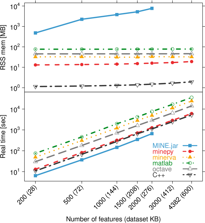
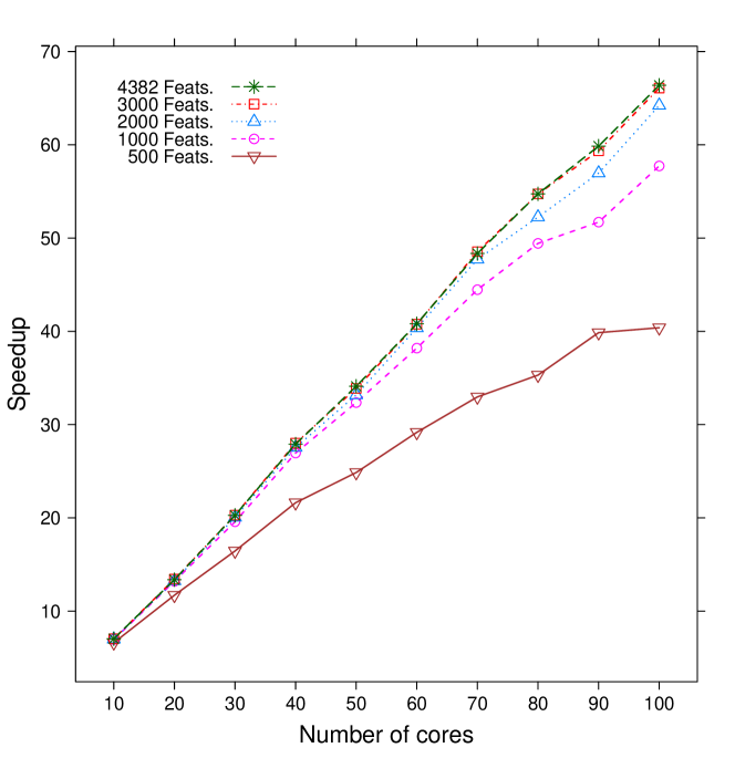
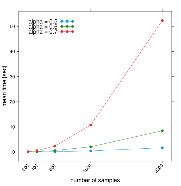
To compare performance for RAM and CPU usage between MINE.jar and the four wrappers, MINE statistics were computed on all features pairs of the Spellman dataset, for increasing feature set sizes (details in SI, Sec 2.2, 2A). Minerva and minepy completed all tasks with limited RAM requirements: about 19 MB were needed for all 4382 variables (600kB dataset size) by minepy, and 2 MB by the C++ interface. We were unable to run MINE.jar with more than 2000 variables, for which Java used 7.5 GB and minepy 16 MB, respectively (Fig. 1, Tab. S2). Minepy computing times are about twice those of the Java solution (Tab. S3), but the speedup is close to 70 for minerva on 100 cores via MPI on a Linux cluster, with the default $\alpha$=0.6 (Fig. S6). Finer grids ($\alpha$=0.7) require much higher computing time as sample size increases (Fig. S7).

We additionally tested the suite on two recent high-throughput transcriptomics datasets, of Affymetrix HumanExon 1.0ST human brain tissues and Illumina Genome Analyzer II sequenced human non-small cell lung cancer (Tab. 6). Details on datasets and experiments are reported in SI.

Performance of minerva and minepy (1-vs.-all) on microarray and RNA-seq datasets listed by GEO accession number. $n$: number of samples. $p$: number of features. CPU: Elapsed time used by the process (in seconds). RAM: resident set size (in kilobytes), for minerva (R) and minepy (P). GEO CPU RAM Acc. no. $n$ $p$ R P R P GSE25219¹ 1,340 17,565 41,880 34,359 533,008 1,509,692 GSE34914² 16 20,422 42 3 35,716 31,956 ¹ Kang et al. (2011)  ² Kalari et al. (2012)

APPENDIX

Appendix A Implementation Details

The core implementation of minepy and minerva is built from scratch in ANSI C starting from the pseudocode provided in Reshef et al. (2011) Supplementary On-line Material (SOM), as no original Java source code is available. The level of detail of the pseudocode leaves a few ambiguities and in this section we list and comment the most crucial choices we adopted for the algorithm steps whenever no explicit description was provided. Obviously, our choices are not necessarily the same as in the original Java version. The occurring differences can be ground for small numerical discrepancies as well as for difference in performance.

1. In SOM, Algorithm 5, the characteristic matrix $M$ is computed in the loop starting at line 7 for $xy\leq B$. This is in contrast with the definition of the MINE measures (see SOM, Sec. 2) where the corresponding bound is $xy<B$ for all the four statistics. We adopted the same bound as in the pseudocode, i.e. $xy\leq B$.

2. The MINE statistic MCN is defined as follows in SOM, Sec. 2:

   $$\textrm{MCN}(D,\epsilon)=\min_{xy<B}\{\log(xy)\colon M(D)_{x,y}\geq(1-\epsilon)\textrm{MIC}(D)\}$$

   As for MINE.jar (inferred from Table S1), we set $\epsilon=0$ and $\log$ to be in base 2. Finally, as specified in Point 1 above, we use the bound $xy\leq B$ as in the SOM pseudocode rather than the $xy<B$ as in the definition. This led to implement the formula:

   $$\textrm{MCN}(D,0)=\min_{xy\leq B}\{\log_{2}(xy)\colon M(D)_{x,y}=\textrm{MIC}(D)\}\,$$

   being $\textrm{MIC}(D)$ the maximum value of the matrix $M(D)$.

3. In EquipartitionYAxis() (SOM, Algorithm 3, lines 4 and 10), two ratios are assigned to the variable desiredRowSize, namely $\frac{n}{y}$ and $\frac{(n-i+1)}{(y-\textrm{currRow}+1)}$. We choose to consider the ratios as real numbers; a possible alternative is to cast desiredRowSize to an integer. The two alternatives can give rise to different $Q$ maps, and thus to slightly different numerical values of the MINE statistics.

4. In some cases, the function EquipartitionYAxis() can return a map $Q$ whose number of clumps $\hat{y}$ is smaller than $y$, e.g. when in $D$ there are enough points whose second coordinates coincide. This can lead to underestimate the normalized mutual information matrix $M_{x,y}$ (SOM, Algorithm 5, line 9), where $M_{x,y}$ is obtained by dividing the mutual information $I_{x,y}$ for $\min\{\log x,\log y\}$. To prevent this issue, we normalize instead by the factor $\min\{\log x,\log\hat{y}\}$.

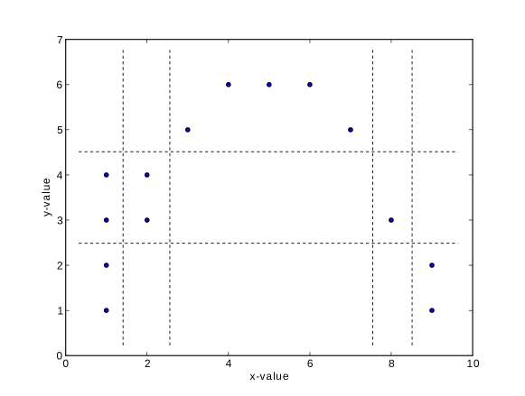
5. The function GetClumpsPartition($D,Q$) is discussed (Reshef et al. (2011), SOM page 12), but its pseudocode is not explicitely available. Our implementation is defined here in Alg. 1. The function returns the map $P$ defining the clumps for the set $D$, with the constraint of keeping in the same clump points with the same $x$-value. An example of $P$ partition produced by GetClumpsPartition on a simple set $D$ is given in Fig. 2.

6. We also explicitly provide the pseudocode for the GetSuperclumpsPartition() function (discussed in Reshef et al. (2011), SOM page 13) in Alg. 2. This function limits the number of clumps when their number $k$ is larger than a given bound $\hat{k}$. The function calls the GetClumpsPartition and, for $k>\hat{k}$ it builds an auxiliary set $D_{\tilde{P}}$ as an input for the EquipartitionYAxis function discussed above (Points 3-4).

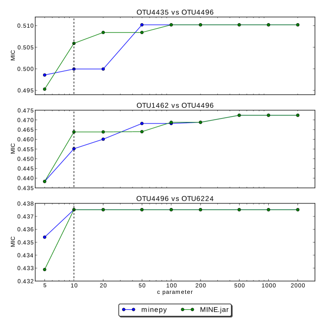
7. We observed that the GetSuperclumpsPartition() implemented in MINE.jar may fail to respect the $\hat{k}$ constraints on the maximum number of clumps and a map $P$ with $\hat{k}+1$ superclumps is actually returned. As an example, the MINE.jar applied in debug mode (d=4 option) with the same parameters ($\alpha=0.551$, $c=10$) used in Reshef et al. (2011) to the pair of variables (OTU4435,OTU4496) of the Microbioma dataset, returns $cx+1$ clumps, instead of stopping at the bound $\hat{k}=cx$ for $x=12,7,6,5,4\ldots$

8. The possibly different implementations of the GetSuperclumpsPartition() function described in Points 6-7 can lead to minor numerical differences in the MIC statistics, as documented in Section 2.1. To confirm this effect, we verified that by reducing the number of calls to the GetSuperclumpsPartition() algorithm, we can also decrease the difference between MIC computed by minepy and by MINE.jar, and they asymptotically converge to the same value. This effect is displayed in Fig. 3, where it is obtained by increasing the value of $c$ in the MIC computation.

9. In our implementation, we use double-precision floating-point numbers (double in C) in the computation of entropy and mutual information values. The internal implementation of the same quantities in MINE.jar is unknown.

10. In order to speed up the computation of the MINE statistics, we introduced two improvements (with respect to the pseudo-code), in OptimizeXAxis(), defined in Algorithm 2 in Reshef et al. (2011) SOM):

    1. Given a $(P,Q)$ grid, we precalculate the matrix of number of samples in each cell of the grid, to speed up the computation of entropy values $H(Q)$, $H(\langle c_{0},c_{s},c_{t}\rangle)$, $H(\langle c_{0},c_{s},c_{t}\rangle,Q)$ and $H(\langle c_{s},c_{t}\rangle,Q)$

    2. We precalculate the entropy matrix $H(\langle c_{s},c_{t}\rangle,Q),\forall s,t$ to speed up the computation of $F(s,t,l)$ (see Algorithm 2, lines 10–17 in Reshef et al. (2011) SOM).

    These improvements do not affect the final results of mutual information matrix and of MINE statistics.

Algorithm 1 GetClumpsPartition($D,Q$)

0:  $D=\{(a_{i},b_{i}),i=1,\dots,n\}$ is a set of $n$ ordered pairs sorted in increasing order by their first component $a_{i}$

0:  $Q$ is the map of row assignments returned by EquipartitionYAxis

0:  Returns a map $P:D\rightarrow\{1,\dots,k\}$ providing the column assignment of the point $(a,b)$

1:  $\tilde{Q}\leftarrow Q$

2:  $i\leftarrow 1$

3:  $c\leftarrow-1$

4:  repeat

5:      $s\leftarrow 0$

6:      $\textit{flag}\leftarrow\textbf{false}{}$

7:      for $j=i+1$ to $n$ do

8:           if $a_{i}=a_{j}$ then

9:               $s\leftarrow s+1$

10:               if $\tilde{Q}((a_{i},b_{i}))\neq\tilde{Q}((a_{j},b_{j}))$ then

11:                    $\textit{flag}\leftarrow\textbf{true}{}$

12:      if $s\neq 0$ and flag then

13:           for $j=0$ to $s$ do

14:               $\tilde{Q}((a_{i+j},b_{i+j}))\leftarrow c$

15:               $c\leftarrow c-1$

16:      $i\leftarrow i+s+1$

17:  until $i>n$

18:  $i\leftarrow 1$

19:  $P((a_{1},b_{1}))\leftarrow i$

20:  for $j=2$ to $n$ do

21:      if $\tilde{Q}((a_{j},b_{j}))\neq\tilde{Q}((a_{j-1},b_{j-1}))$ then

22:           $i\leftarrow i+1$

23:      $P((a_{j},b_{j}))\leftarrow i$

24:  return  $P$

Algorithm 2 GetSuperclumpsPartition($D,Q,\hat{k}$)

0:  $D=\{(a_{i},b_{i}),i=1,\dots,n\}$ is a set of $n$ ordered pairs sorted in increasing order by their first component $a_{i}$

0:  $Q$ is the map of row assignments returned by EquipartitionYAxis

0:  $\hat{k}$ is the maximum number of clumps

0:  Returns a map $P:D\rightarrow\{1,\dots,k\}$ providing the column assignment of the point $(a,b)$

1:  $\tilde{P}\leftarrow$ GetClumpsPartition($D,Q$)

2:  $k\leftarrow$ number of clumps of $\tilde{P}$

3:  if $k>\hat{k}$ then

4:      $D_{\tilde{P}}\leftarrow\{(0,\tilde{P}((a_{i},b_{i}))):(a_{i},b_{i})\in D\}$

5:      $\hat{P}\leftarrow$ EquipartitionYAxis($D_{\tilde{P}},\hat{k}$)

6:      $P((a_{i},b_{i}))\leftarrow\hat{P}((0,\tilde{P}((a_{i},b_{i}))))$ for every $(a_{i},b_{i})$

7:      return  $P$

8:  else

9:      return  $\tilde{P}$

D Q P (1,1) 1 1 (1,2) 1 1 (1,3) 2 1 (1,4) 2 1 (2,3) 2 2 (2,4) 2 2 (3,5) 3 3 (4,6) 3 3 (5,6) 3 3 (6,6) 3 3 (7,5) 3 3 (8,3) 2 4 (9,2) 1 5 (9,1) 1 5

Figure 2: Example of application of the GetClumpsPartition function on the set D: first we apply the EquipartitionYAxis(D,y) function with $y=3$ and then the GetClumpsPartition(D,Q), obtaining the map $P$. Left: the dataset $D$ and the grid cells. Right: mapping of points in $D$ for $Q$ ($y$-axis partition) and $P$ ($x$-axis partition).

Figure 3: Microbioma dataset. Comparison between MINE.jar and minepy for increasing values of the $c$ parameter for the first three feature pairs of Tab. 1. The parameter $c=10$ actually used in the experiment is indicated by dashed vertical lines, for which MIC differences are found between minepy and MINE.jar (top and middle panels). For larger $c$ values the two implementations converge to the same MIC statistic.

Appendix B Comparison with MINE.jar

B.1 Consistency

1A

Minepy was compared with the original MINE.jar implementation on a “one vs all” MINE association study on the Spellman dataset. In this task, MINE statistics were computed for variable #1 (time) vs. all the other 4381 variables, with grid parameter $\alpha$$=$0.67 and $c$$=$15, as in Reshef et al. (2011). MIC values for the two implementations are compared in Fig. 4: all values coincide up to five digit precision, i.e. the precision of MINE.jar output. Specifications of hardware and software configurations for this and the other experiments described in this document are summarized in Sec. D.

Figure 4: A comparison of MIC values for minepy (x axis) and the original MINE.jar (y axis) on the Spellman dataset (time vs. all the other 4381 variables). Parameters are $\alpha$=0.67 and $c$$=$15 for both implementations.

1B

The MINE analysis was run for all feature pairs with minepy on the microbiome dataset (6696 features) with $\alpha=0.551$ and $c=10$, as chosen in Reshef et al. (2011). MIC values were compared with the 77 top ranked associations from Tab S13, Supp. Mat. in Reshef et al. (2011). MIC values are identical in 44 cases, for 73 the difference is less than 0.01. The median of all differences is 0, the 3rd quartile is 0.003, and the largest observed difference is 0.014; all comparisons are listed in Tab. 1.

OTUX	OTUY	J	P	OTUX	OTUY	J	P
OTU4435	OTU4496	0.506	0.500	OTU453	OTU4496	0.282	0.284
OTU1462	OTU4496	0.464	0.455	OTU1347	OTU5937	0.300	0.290
OTU4496	OTU6224	0.438	0.438	OTU2728	OTU5937	0.276	0.276
OTU155	OTU4496	0.425	0.425	OTU2970	OTU6256	0.289	0.289
OTU4496	OTU5417	0.414	0.414	OTU1629	OTU3991	0.292	0.292
OTU675	OTU5937	0.414	0.412	OTU4865	OTU5937	0.321	0.321
OTU2728	OTU4496	0.408	0.408	OTU3991	OTU4273	0.266	0.266
OTU5417	OTU5937	0.408	0.410	OTU2350	OTU6256	0.272	0.272
OTU4273	OTU4496	0.374	0.372	OTU2941	OTU6256	0.280	0.280
OTU675	OTU6256	0.362	0.357	OTU5420	OTU5937	0.432	0.431
OTU1629	OTU6256	0.374	0.374	OTU4496	OTU4501	0.259	0.259
OTU2970	OTU4496	0.358	0.357	OTU1285	OTU4496	0.256	0.256
OTU4273	OTU5937	0.366	0.366	OTU5407	OTU5420	0.272	0.275
OTU710	OTU4496	0.354	0.354	OTU3991	OTU4435	0.251	0.251
OTU4257	OTU6256	0.346	0.355	OTU5826	OTU6256	0.251	0.252
OTU4257	OTU4496	0.339	0.325	OTU1285	OTU5937	0.296	0.286
OTU1193	OTU4496	0.336	0.342	OTU4496	OTU5826	0.255	0.255
OTU2642	OTU2728	0.385	0.383	OTU4865	OTU6256	0.249	0.249
OTU1373	OTU4496	0.322	0.322	OTU6256	OTU6484	0.247	0.247
OTU4273	OTU6256	0.329	0.335	OTU4496	OTU6484	0.247	0.247
OTU1462	OTU3991	0.326	0.326	OTU1629	OTU5937	0.266	0.267
OTU2941	OTU4496	0.332	0.332	OTU4865	OTU5407	0.245	0.245
OTU2728	OTU5490	0.353	0.353	OTU4496	OTU4865	0.252	0.252
OTU4496	OTU5420	0.312	0.318	OTU2399	OTU2728	0.244	0.244
OTU1629	OTU4496	0.305	0.305	OTU2399	OTU5420	0.250	0.250
OTU5937	OTU6224	0.301	0.293	OTU2516	OTU4496	0.253	0.253
OTU2350	OTU4496	0.302	0.302	OTU5117	OTU6256	0.243	0.243
OTU1347	OTU6256	0.329	0.320	OTU5826	OTU5937	0.264	0.264
OTU675	OTU4496	0.296	0.294	OTU4435	OTU5937	0.244	0.245
OTU4496	OTU5117	0.291	0.291	OTU2728	OTU5407	0.239	0.242
OTU1285	OTU6256	0.287	0.287	OTU2036	OTU6256	0.236	0.236
OTU1347	OTU4496	0.291	0.286	OTU774	OTU1347	0.236	0.236
OTU4496	OTU5370	0.291	0.290	OTU2970	OTU3991	0.236	0.232
OTU3994	OTU5937	0.285	0.277	OTU3991	OTU5370	0.235	0.235
OTU3994	OTU4496	0.294	0.294	OTU155	OTU6256	0.251	0.251
OTU4257	OTU5937	0.379	0.369	OTU4501	OTU6256	0.232	0.224
OTU710	OTU5937	0.296	0.290	OTU453	OTU3991	0.241	0.235
OTU1373	OTU5937	0.281	0.281	OTU1548	OTU4496	0.234	0.234
OTU1548	OTU6256	0.277	0.277

Table 1: Side by side comparison (J: MINE.jar; P: minepy) for the 77 top ranked MIC (OTUX,OTUY) pairs from Tab. S13 of Reshef et al. (2011) SOM.

B.2 Performance

2A.

We compared the computing performance of the C MINE wrappers (minepy, minerva, the MATLAB/Octave and the C++ interfaces) with MINE.jar on the CDC15 Spellman dataset. A MINE analysis (four MINE statistics, Pearson and non-linearity) was run on all feature pairs for all the 23 time points and increasing feature set sizes. Results are for memory and elapsed computing times are summarized in Fig. 1 (main paper) and here reported in Tab. 2 and Tab. 3 respectively.

In terms of computing time, MINE.jar has a good performance (See Fig. 1, bottom panel), but it requires a much larger amount of memory. With the default parameters, which correspond to reserving 3GB to the process, we were unable to complete tasks for 1,500 or more features with MINE.jar (OutOfMemoryError exception). On the 12 GB RAM system used in this experiment, we then reserved 8 GB by using the -Xmx option (suggested on MINE website, FAQ section). With this configuration, MINE.jar used 5.1 GB and 7.5 GB RAM for 1500 and 2000 variables respectively, then stopped at about 2.7 $\times 10^{6}$ comparisons without completing the task.

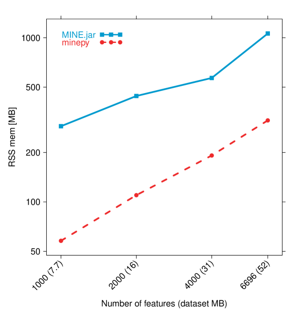
In comparison, memory requirement for our MINE implementations grows much slower on the Spellman dataset. Indeed, the C++ interface has the lowest memory footprint (less than 2 MB for 4382 variables). For the Python, R, MATLAB and Octave interfaces, memory is mostly used by the environments. On the much more numerous Microbiome dataset (675 samples), memory usage of minepy is consistently smaller than MINE.jar for a MINE analysis on variable 1 vs all variables, as shown in Tab. 4 and Fig. 5.

Num	Dataset	MINE.jar	minepy	minerva	matlab	octave	C++
Feat	(kB)
200	28	480.62	13.05	32.38	76.75	45.41	1.14
500	72	2,242.00	13.61	32.68	76.82	45.46	1.21
1,000	144	3,798.57	14.31	31.20	76.90	45.55	1.30
1,500	208	5,218.90	15.15	31.35	77.24	45.64	1.39
2,000	276	7,670.30	15.98	33.17	77.47	45.73	1.49
3,000	412	–	17.04	32.48	78.12	45.90	1.67
4,382	600	–	19.10	32.38	78.10	46.14	1.94

Table 2: Memory usage, evaluated as resident set size (MB), i.e. the non-swapped physical memory used by the task, for MINE.jar, minepy, minerva, MATLAB, Octave, C++.

Num	Dataset	MINE.jar	minepy	minerva	matlab	octave	C++
Feat	(kB)
200	28	6	13	49	75	30	11
500	72	37	82	311	461	180	68
1,000	144	146	320	1,224	1,976	718	280
1,500	208	349	718	2,825	4,161	1,621	653
2,000	276	664	1,275	4,936	7,617	2,869	1,119
3,000	412	–	2,885	11,185	16,689	6,467	2,457
4,382	600	–	6,115	24,307	35,810	14,147	5,199

Table 3: Computing time comparisons (secs) for MINE.jar, minepy, minerva, MATLAB, Octave and C++ interfaces, on the Spellman dataset (all pairs); as elapsed real (wall clock) time used by the process.

Num	Dataset	MINE.jar	minepy
Feat	Dim (MB)
1,000	8	295,984	59,332
2,000	16	452,356	112,536
4,000	31	582,480	196,352
6,696	52	1,086,504	321,184

Table 4: Comparison of memory usage (kB) for MINE.jar and minepy computing the four MINE statistics, the Pearson correlation coefficient and the non linearity index for variable 1 versus all of the Microbiome dataset. Memory is evaluated as resident set size (RSS), i.e. the non-swapped physical memory used by the task, for increasing number of features.

Figure 5: Comparison of memory usage of MINE.jar and minepy computing the four MINE statistics, the Pearson correlation coefficient and the non linearity index for variable 1 versus all of the Microbiome dataset. In parentheses, the dataset ASCII file size in megabytes (MB).

We also evaluated on the same data the effect of enabling parallelization in minerva. This can be managed natively in R by using functionalities of the parallel package R Core Team (2012). An example of how to enable multicore computation is:

> # load the minerva package
> library(minerva)
> # load the Spellman dataset (available in minerva)
> data(Spellman)
> # run MINE on variable ‘‘time’’ vs all, with 8 cores
> res <- mine(x=Spellman, master=1, alpha=0.67, C=15, n.cores=8)

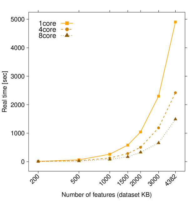
In the experiment we computed the MINE statistics with 1, 4, or 8 cores for all pairs of features of the Spellman dataset, obtaining the plot in Fig. 6. For 4382 features, computing time is reduced from about 5000 secs with one core to 1500 with 8 cores.

Figure 6: Elapsed time used by the process (in seconds) versus increasing number of features (log scale) to compute the MINE statistics for all pairs of features of the CDC15 Spellman yeast dataset.

2B.

To evaluate scalability, an experiment of MPI parallelization of minerva was performed with the Rmpi package on the high-performance Linux computing cluster FBK-KORE. Up to 100 cores (described in Subsection D.2) were employed in the tests, managed by the Sun Grid Engine (SGE) batch-queuing system. The MINE analysis (four MINE statistics) was applied to 5 instances of the Spellman dataset, in “all vs all” mode and 10 different configurations with increasing number of cores up to 100. Speedup was defined as: $\textrm{Speedup}(p)=T_{1}/T_{p}$, where $T_{p}$ is the time cost of the algorithm on $p$ processes. As in 2A, computing time was considered as wall clock time.

The speedup is higher for larger datasets, with the curve for 4382 features almost overlapping that for 3000 (saturation effect). A speedup of about 70 was achieved with 100 cores for 4382 features. Results are displayed in Fig. 7.

Figure 7: Speedup plot for increasing number of cores from 10 to 100. The MINE statistics were computed for all pairs and increasing feature set sizes on the CDC15 Spellman yeast dataset ($\alpha$=0.6).

2C.

The scaling properties of MINE as a function of the sample size $n$ and the $\alpha$ parameter are important in practical applications. As introduced in Reshef et al. (2011), $\alpha$ defines the maximum grid size $B$ according to the relation $B(n)=n^{\alpha}$. Finer grids correspond obviously to higher computational costs. We empirically evaluated how computing time grows for varying $\alpha$ and $n$ by considering a MINE analysis for two variables on datasets of increasing size, here simulated by two uniformly distributed random vectors of increasing length. The R interface minerva was applied on a standard laptop system (sw and hw details in Sec. D.3).

Fig. 8 displays the mean elapsed time for 100 replicates for 5 different sample sizes. The results confirm how critical is the choice of $\alpha$ on computing time: the standard $\alpha=0.6$ proposed in Reshef et al. (2011) requires less than 15% of the time needed for $\alpha=0.7$.

Due to the linearity in computing MINE statistics on $p$ pairs of variables, Fig. 8 can be used to derive a rough estimate of the total time required to perform a MINE computation on a given dataset.

Figure 8: Average of elapsed time on 100 repetitions of MINE analysis with the minerva package on two uniformly distributed random variables for an increasing number of samples and $\alpha=0.5,0.6,\textrm{and }0.7$.

Appendix C Transcriptomic datasets

In this section, we describe the high-throughput transcriptomic datasets used for the additional experiments reported in Tab. 1 of the main paper. In both experiments, we set $c=15$ and $\alpha=0.6$; hardware and software configurations are specified in Subsection D.4.

3A

Human brain transcriptome dataset (GSE25219). This exon array dataset Kang et al. (2011) was obtained from 1340 samples, collected from multiple regions of 57 postmortem human brains, spanning from embryonic development to late adulthood, 31 males and 26 females of different ethnicities. The samples were spotted on a Affymetrix Human Exon 1.0 ST Array, and core and unique probe sets were summarized, representing 17,565 mainly protein-coding genes, into gene-level information (transcript gene version). Note that at the same accession number GSE25219 an exon version of the data is also provided, but we used the gene version for Tab. 1 of the main paper. For replicability, the dataset formatted for the MINE analysis is available at http://sourceforge.net/projects/minepy/files/data/GSE25219.csv.

3B

Non-small cell lung cancer RNA-seq dataset (GSE34914). The data were generated by an RNA-sequencing study of non-small cell lung cancer (NSCLC) Kalari et al. (2012). The cohort includes 8 lung adenocarcinomas with mutant KRAS in lung tumors and 8 lung adenocarcarcinomas without KRAS mutation. One tumor sample without KRAS mutation was run twice for QC evaluation. The samples were sequenced on an Illumina Genome Analyzer II. The raw read counts from BWA alignment are available for 22,316 genes, but we filtered out 1,894 features having variance smaller than $10^{-5}$. For replicability, the dataset formatted for the MINE analysis is available at http://sourceforge.net/projects/minepy/files/data/GSE34914.csv.

Appendix D Hardware/Software configurations

D.1 Experiments: 1A, 2A

• 8 cores Intel^® Xeon^® E5540 2.53 GHz 64 bit workstation (“krk”), with 12 GB RAM

• Linux 2.6.18

• Red Hat 4.1.2

• GCC 4.1.2

• Java^™ 1.7.0

• Python 2.7.3 and NumPy 1.6.2

• R 2.15.1

• MATLAB^® 7.6.0.324 (R2008a)

• GNU Octave 3.0.5

• MINE.jar 1.0.1

• minepy 0.3.5

• minerva 1.1

D.2 Experiments: 1B, 2B

These experiments were run on a high-performance computing Linux cluster (“FBK-KORE”), with more than 700 cores and 200 TB disk space. A queue was reserved for the experiments, in which each computing node was equipped with:

• quad-core Intel^® Xeon^® E5420 2.5 GHz, reserving 2 GB RAM

• Red Hat 4.4.6-4

• GCC 4.4.6

• Open MPI 1.5.4

• Rmpi 0.6-1

• Python 2.7.3 and NumPy 1.6.1

• R 2.15.1

• minepy 0.3.5

• minerva 1.1

D.3 Experiment: 2C

• Intel^® Core^™ 2 Duo 3.06 GHz laptop (“Dna”) with 4GB RAM

• Mac OS X Lion 10.7.4

• GCC 4.2.1 (Based on Apple Inc. build 5658) (LLVM build 2336.9.00)

• R 2.15.1

• minerva 1.1

D.4 Experiments: 3A, 3B

• 24 core Intel^® Xeon^® E5649 CPU 2.53GHz workstation (“mlbio”) with 47 GB RAM

• Linux 2.6.32

• Red Hat 4.4.6

• GCC 4.4.6

• Java 1.7.0

• Python 2.6.6 and Numpy 1.6.0

• R 2.15.1

• MINE.jar 1.0.1

• minepy 0.3.5

• minerva 1.1

Appendix E Examples

We provide in this section examples of usage of interfaces based on the libmine C library. All datasets considered in this section are available at http://sourceforge.net/projects/minepy/files/data, and at the MINE website http://www.exploredata.net. All examples are based on minepy 0.3.5 and minerva 1.1.

E.1 Spellman dataset

In this example we will first compute the MINE statistics on the Spellman dataset, analyzing the association between variable “time” and each of the other variables, printing the MIC value of “time” vs “YAL001C”. We use the same parameter configuration as in Reshef et al. (2011): $\alpha=0.67$ and $c=15$. The dataset is available at
http://sourceforge.net/projects/minepy/files/data/Spellman.csv or within the minerva package for R users.

E.1.1 Python API (included in minepy)

Download and install the latest minepy module from the project page (http://minepy.sourceforge.net).

>>> # import the numpy module
>>> import numpy as np
>>> # import the minepy module
>>> from minepy import MINE
>>> # load the Spellman dataset
>>> spellman = np.genfromtxt(’Spellman.csv’, delimiter=’,’)[:, 1:]
>>> # initialize results values with an empty list
>>> res = []
>>> for i in range(1, len(spellman)):
...     # build the mine object
...     mine = MINE(alpha=0.67, c=15)
...     # compute the MINE statistics
...     mine.score(spellman[0], spellman[i])
...     res.append(mine)
...
>>> # print MIC of ’time’ vs ’YAL001C’
>>> res[0].mic()
0.6321377231641834

E.1.2 mine Application (included in minepy)

Download and install the latest mine application from the minepy homepage (http://minepy.sourceforge.net).

$ mine Spellman.csv -a 0.67 -c 15 -m 1 -o Spellman_MINE.txt

The MINE statistics will be stored in the Spellman_MINE.txt file.

E.1.3 R API (minerva)

Download and install the latest minerva package from CRAN
(http://cran.r-project.org/web/packages/minerva/index.html).

> # load the minerva package
> library(minerva)
> # load the Spellman dataset
> data(Spellman)
> # compute the MINE statistics
> res <- mine(x=Spellman, master=1, alpha=0.67, C=15)
> # print ’time’ vs ’YAL001C’
> res[["MIC"]]["YAL001C",]
[1] 0.6321377

E.1.4 MATLAB/Octave API (included in minepy library)

Download and install the MATLAB interface from the latest minepy package (http://minepy.sourceforge.net).

>> % load the Spellman dataset
>> spellman = csvread(’Spellman.csv’, 0, 1);
>> n = length(spellman);
>> % preallocate and initialize to zero the results array
>> res(1:n-1) = struct(’mic’,0,’mas’,0,’mev’,0,’mcn’,0);
>> % compute the MINE statistics
>> for i = 2:n
res(i-1) = mine(spellman(1,:),spellman(i,:), 0.67, 15);
end
>> % print ’time’ vs ’YAL001C’
>> res(1)

ans =

    mic: 0.6321
    mas: 0.2537
    mev: 0.6321
    mcn: 3

E.2 Microbiome dataset

In this example we will compute the MINE statistics (“all vs all” study) on the Microbiome dataset by using the mine Application. We use the parameter configuration $\alpha=0.551$ and $c=10$. The dataset is available at
http://sourceforge.net/projects/minepy/files/data/Microbiome.csv.

Note that in this experiment the computational time may be very high on a standard workstation. First download and install the latest minepy package from http://minepy.sourceforge.net. To launch the analysis:

$ mine Microbiome.csv -a 0.551 -c 10 -o Microbiome_MINE.txt

To compute the MINE statistics between variable #100 versus all the others we can use the “master variable” option (-m):

$ mine Microbiome.csv -a 0.551 -c 10 -m 100 -o Microbiome_MINE.txt

The MINE statistics between variables #100 and #200 can be also directly computed by using the “pair” option (-p):

$ mine Microbiome.csv -a 0.551 -c 10 -p 100 200 -o Microbiome_MINE.txt

Output statistics for the examples above will be stored in the Microbiome_MINE.txt file.

E.3 Baseball dataset

In this example we will compute the MINE statistics (“all vs all” mode) on the Baseball dataset with the mine Application with $\alpha=0.7$ and $c=15$. The dataset is available at
http://sourceforge.net/projects/minepy/files/data/MLB2008.csv. Note that in this experiment the computational time may be very high on a standard workstation. First download and install the latest minepy package from http://minepy.sourceforge.net. To launch the analysis:

$ mine MLB2008.csv -a 0.7 -c 15 -o MLB2008_MINE.txt

The statistics will be stored in the MLB2008_MINE.txt file.

E.4 C++ example

In this example we will compute the MINE statistics between $x=\{0,0.001,\dots,1\}$ and $y=\sin(10\pi x)+x$. Download and untar the latest minepy module from the project page (http://minepy.sourceforge.net). This example is located in minepy-X.Y.Z/examples/cpp_example.cpp (where X.Y.Z is the current version of minepy).

#include <cstdlib>
#include <cmath>
#include <iostream>
#include "cppmine.h"

using namespace std;

int
main (int argc, char **argv)
{
  double PI;
  int i, n;
  double *x, *y;
  MINE *mine;

  PI = 3.14159265;

  /* build the MINE object with exceptions management */
  try {
    mine = new MINE(0.6, 15);
  }
  catch (char *s) {
      cout << "WARNING: " << s << "\n";Ψ
      cout << "MINE will be set with the default parameters," << "\n";
      cout << "alpha=0.6 and c=15" << "\n";
      mine = new MINE(0.6, 15);
  }

  /* build the problem */
  n = 1001;
  x = new double [n];
  y = new double [n];
  for (i=0; i<n; i++)
    {
      /* build x = [0, 0.001, ..., 1] */
      x[i] = (double) i / (double) (n-1);

      /* build y = sin(10 * pi * x) + x */
      y[i] = sin(10 * PI * x[i]) + x[i];
    }

  /* compute score */
  mine->compute_score(x, y, n);

  /* print mine statistics */
  cout << "MIC: " << mine->get_mic() << "\n";
  cout << "MAS: " << mine->get_mas() << "\n";
  cout << "MEV: " << mine->get_mev() << "\n";
  cout << "MCN: " << mine->get_mcn() << "\n";

  /* delete the mine object */
  delete mine;

  /* free the problem */
  delete [] x;
  delete [] y;

  return 0;
}

On a standard Linux machine, open a terminal, go into the example folder (examples/) and compile the code:

$ g++ -O3 -Wall -Wno-write-strings cpp_example.cpp \
../minepy/libmine/cppmine.cpp ../minepy/libmine/core.c \
 ../minepy/libmine/mine.c -I../minepy/libmine/

Run the example by typing:

$ ./a.out
MIC: 0.999999
MAS: 0.728144
MEV: 0.999999
MCN: 4.584963

E.5 Other examples

Short examples are available in the on line documentation about the APIs and the mine application at: http://minepy.sourceforge.net/docs. For example, for v0.3.5, the examples can be found at:

• : http://minepy.sourceforge.net/docs/0.3.5/python.html

• : http://minepy.sourceforge.net/docs/0.3.5/c.html

• : http://minepy.sourceforge.net/docs/0.3.5/cpp.html

• : http://minepy.sourceforge.net/docs/0.3.5/matlab.html

• : http://minepy.sourceforge.net/docs/0.3.5/application.html

For minerva, the most updated documentation and examples are available at

• : http://cran.r-project.org/web/packages/minerva/minerva.pdf

References

- Anderson et al. (2012) Anderson, T., Laegreid, W., Cerutti, F., Osorio, F., Nelson, E., Christopher-Hennings, J., and Goldberg, T. (2012). Ranking viruses: measures of positional importance within networks define core viruses for rational polyvalent vaccine development. Bioinformatics, 28(12), 1624–1632.
- Das et al. (2012) Das, J., Mohammed, J., and Yu, H. (2012). Genome-scale analysis of interaction dynamics reveals organization of biological networks. Bioinformatics, 28(14), 1873–1878.
- Faust and Raes (2012) Faust, K. and Raes, J. (2012). Microbial interactions: from networks to models. Nature Rev Microbiol, 10, 538–550.
- Kalari et al. (2012) Kalari, K., Rossell, D., Necela, B., Asmann, Y., Nair, A., Baheti, S., Kachergus, J., Younkin, C., Baker, T., Carr, J., Tang, X., Walsh, M., Chai, H., Sun, Z., Hart, S., Leontovich, A., Hossain, A., Kocher, J.-P., Perez, E., Reisman, D., Fields, A., and Thompson, E. (2012). Deep Sequence Analysis of Non-Small Cell Lung Cancer: Integrated Analysis of Gene Expression, Alternative Splicing, and Single Nucleotide Variations in Lung Adenocarcinomas with and without Oncogenic KRAS Mutations. Front Oncol, 2, 12.
- Kang et al. (2011) Kang, H., Kawasawa, Y., Cheng, F., Zhu, Y., Xu, X., Li, M., Sousa, A., Pletikos, M., Meyer, K., Sedmak, G., Guennel, T., Shin, Y., Johnson, M., Krsnik, Z., Mayer, S., Fertuzinhos, S., Umlauf, S., Lisgo, S., Vortmeyer, A., Weinberger, D., Mane, S., Hyde, T., Huttner, A., Reimers, M., Kleinman, J., and Sestan, N. (2011). Spatio-temporal transcriptome of the human brain. Nature, 478(7370), 483–489.
- Karpinets et al. (2012) Karpinets, T., Park, B., and Uberbacher, E. (2012). Analyzing large biological datasets with association networks. Nucleic Acids Research, 40(17), e131.
- Nat. Biotech. (2012) Nat. Biotech. (2012). Finding correlations in big data. Nat Biotech, 30(4), 334–335.
- R Core Team (2012) R Core Team (2012). R: A Language and Environment for Statistical Computing. R Foundation for Statistical Computing, Vienna, Austria. ISBN 3-900051-07-0.
- Reshef et al. (2011) Reshef, D., Reshef, Y., Finucane, H., Grossman, S., McVean, G., Turnbaugh, P., Lander, E., Mitzenmacher, M., and Sabeti, P. (2011). Detecting novel associations in large datasets. Science, 6062(334), 1518–1524.
- Speed (2011) Speed, T. (2011). A Correlation for the 21st Century. Science, 6062(334), 1502–1503.
- Spellman et al. (1998) Spellman, P., Sherlock, G., Zhang, M., Iyer, V., Anders, K., Eisen, M., Brown, P., Botstein, D., and Futcher, B. (1998). Comprehensive identification of cell cycle-regulated genes of the yeast Saccharomyces cerevisiae by microarray hybridization. Mol Biol Cell, 9(12), 3273–3297.
- Weiss et al. (2012) Weiss, J., Karma, A., W.R., M., Deng, M., Rau, C., Rees, C., Wang, J., Wisniewski, N., Eskin, E., Horvath, S., Qu, Z., Wang, Y., and Lusis, A. (2012). ”Good enough solutions” and the genetics of complex diseases. Circ Res, 111(4), 493–504.