Robust Distributed Maximum Likelihood Estimation with Dependent Quantized Data

Abstract

In this paper, we consider distributed maximum likelihood estimation (MLE) with dependent quantized data under the assumption that the structure of the joint probability density function (pdf) is known, but it contains unknown deterministic parameters. The parameters may include different vector parameters corresponding to marginal pdfs and parameters that describe dependence of observations across sensors. Since MLE with a single quantizer is sensitive to the choice of thresholds due to the uncertainty of pdf, we concentrate on MLE with multiple groups of quantizers (which can be determined by the use of prior information or some heuristic approaches) to fend off against the risk of a poor/outlier quantizer. The asymptotic efficiency of the MLE scheme with multiple quantizers is proved under some regularity conditions and the asymptotic variance is derived to be the inverse of a weighted linear combination of Fisher information matrices based on multiple different quantizers which can be used to show the robustness of our approach. As an illustrative example, we consider an estimation problem with a bivariate non-Gaussian pdf that has applications in distributed constant false alarm rate (CFAR) detection systems. Simulations show the robustness of the proposed MLE scheme especially when the number of quantized measurements is small.

, ,

1 Introduction

Wireless sensor networks have attracted much attention with a lot of research taking place over the past several years. Many advances have been made in distributed detection, estimation, tracking and control (see e.g., [16] and references therein). Distributed estimation and quantization problems have been considered in a number of previous studies. The parameters to be estimated are modeled as random and deterministic in different situations. For random parameters, there exist various prior studies under the assumption of known joint pdf of parameters and sensor measurements (see, e.g., [9]). We concentrate on deterministic parameters in this paper. For deterministic parameters, several universal distributed estimation schemes have been proposed [19] in the presence of unknown, additive sensor noises that are bounded and identically distributed. The work in [11] addressed design and implementation issues under the assumption of a scalar parameter to be estimated and using scalar quantizers. The work in [4] proposed vector quantization design for distributed estimation under the assumption of additive observation noise model.

System identification based on quantized measurements is a challenging problem even for very simple models and has been researched for a wide range of applications (see, e.g., [17]). A method for recursive identification of the nonlinear Wiener model was developed in [18] and the corresponding convergence properties were analyzed. In [5], Godoy et al. developed an MLE approach and used a scenario-based form of the expectation maximization algorithm to parameter estimation for general MIMO FIR linear systems with quantized outputs. The problem of set membership system identification with quantized measurements was considered in [2]. In [6], the results from statistical quantization theory were surveyed and applied to both moment calculations and the likelihood function of the measured signal. The system identification of ARMA models using intermittent and quantized output observations was proposed in [8]. The formal conditions for the asymptotic normality of the MLE to the reliability of a complex system based on a combination of full system and subsystem tests were proposed in [12].

In previous works, the MLE with quantized data is extensively used to estimate the deterministic parameters. In this paper, robust distributed MLE with dependent quantized data is considered. Our work differs from previous studies in several aspects. Previous results concentrate on the problem of how to design the quantization schemes for estimating a deterministic parameter where each sensor makes one noisy observation. The observations are usually assumed independent across sensors, and they discuss the relationship between MLE performance and the number of sensors. Here, we focus on the problem of how to design estimation schemes for the unknown parameter vector associated with the joint pdf of the observations where the number of sensors is fixed. The emphasis here is on system robustness. These observations may be dependent across sensors. The unknown parameters may include different vector parameters corresponding to marginal pdfs and parameters that describe dependence of observations across sensors. Actually, the dependence between sensors is very important in multisensor fusion systems, for example, see the recent work on distributed location estimation with dependent sensor observations [13].

In this paper, we investigate the performance of MLE with multiple quantizers, since MLE with a single quantizer is sensitive to the choice of thresholds due to the uncertainty of pdf (see, e.g., [3]). Our main contribution is that we analytically derive the asymptotic efficiency and robustness of a practical MLE with multiple quantizers in the context of dependent quantized measurements at the sensors, unknown parameter vector and without the knowledge of measurement models. The difficulties include the fact that due to dependence between measurements across sensors, the unknown high dimensional vector parameter estimation problem cannot be decoupled to scalar parameter estimation problems; and the quantized samples are not identically distributed due to the use of multiple different quantizers. Therefore, we have to deal with unknown vector parameter and unidentically distributed samples simultaneously. The asymptotic variance is derived to be the inverse of a weighted linear combination of Fisher information matrices based on $J$ different quantizers which can be used to verify the robustness of our approach. A typical estimation problem with a bivariate non-Gaussian pdf with application to the distributed CFAR detection systems is considered. Simulations show that the new MLE scheme is robust and much better than that based on the worst quantization scheme from among the groups of quantizers. Moreover, when the number of quantized measurements is small, a surprising result is that the robust MLE has a significant and dominated advantage over the MLE with a single quantizer. It is also shown that the performance of the robust MLE is not the average performance of multiple quantizers. The rest of the paper is organized as follows. Problem formulation is given in Section 2. In Section 3, the robust MLE scheme is proposed and the asymptotic results are derived. In Section 4, numerical examples are given and discussed. In Section 5, conclusions are made.

2 Problem formulation

The basic $L$-sensor distributed estimation system is considered (see Figure 1). Each sensor has $k_{i}$-dimensional observation population $Y_{i}$, $i=1,\ldots,L$. Suppose that the joint observation population $Y\triangleq(Y_{1}^{\prime},\ldots,Y_{L}^{\prime})^{\prime}$ has a given family of joint pdf:

$$\{p(y_{1},\ldots,y_{L}|\theta)\}_{\theta\in\Theta\subseteq\mathbb{R}^{k}}$$ (1)

where ^′ denotes the transpose and $\theta$ is the unknown $k$-dimensional deterministic parameter vector which may include marginal parameters and dependence parameters. Here, we do not assume independence across sensors, knowledge of measurement models and Gaussianity of the joint pdf. Let $N$ independently and identically distributed (i.i.d.) sensor observation samples and joint observation samples be

$$\vec{Y}_{i} = (Y_{i1},\ldots,Y_{iN}),~{}i=1,\ldots,L;$$ (2)

$$\vec{Y} = (\vec{Y}_{1}^{\prime},\ldots,\vec{Y}_{L}^{\prime})^{\prime}.$$ (3)

Figure 1: Distributed MLE fusion system with quantized data

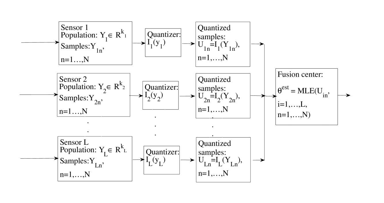
Suppose the sensors and the fusion center wish to jointly estimate the unknown parameter vector $\theta$ based on the spatially distributed observations. If there is sufficient communication bandwidth and power, the fusion center can obtain asymptotically efficient estimates with the complete observation samples based on MLE procedure under some regularity conditions on the joint pdf.

In many practical situations, however, to reduce the communication requirement from sensors to the fusion center due to limited communication bandwidth and power, the $i$-th sensor quantizes the observation vector to 1 bit (it is straightforward to extend to multiple bits) by a measurable indicator quantization function:

$$I_{i}(y_{i}):~{}y_{i}\in\mathbb{R}^{k_{i}}\rightarrow\{0,1\},$$ (4)

for $i=1,\ldots,L$. Here, the quantization region of each quantizer $I_{i}(y_{i})$ may be continuous or union of discontinuous regions. Moreover, we denote by

$$I(y)\triangleq(I_{1}(y_{1}),\ldots,I_{L}(y_{L}))^{\prime}\in\mathbb{R}^{L}.$$ (5)

Once the binary quantized samples $I_{i}(Y_{in})$ are generated at sensor $i$, $i=1,\ldots,L$, they are transmitted to the fusion center, for $n=1,\ldots,N$. The fusion center is then required to estimate the true parameter vector $\theta^{*}$ based on the received quantized data. By the definition of observation samples and quantizers, we define

$$\vec{U} \triangleq (\vec{U}_{1}^{\prime},\ldots,\vec{U}_{N}^{\prime})^{\prime},$$ (6)

$$\vec{U}_{n} \triangleq (U_{1n},\ldots,U_{Ln})^{\prime},~{}n=1,\ldots,N,$$ (7)

$$U_{in} \triangleq I_{i}(Y_{in}),~{}n=1,\ldots,N.$$ (8)

If we take $\vec{U}_{n}$ as the joint quantized observation sample and denote the quantized observation population by $U\triangleq I(Y)$ $=(I_{1}(Y_{1}),$ $\ldots$, $I_{L}(Y_{L}))^{\prime}$, we know that $U$ has a discrete/categorical distribution. Based on the pdf of $Y$ and quantizers $I(y)$, the probability mass function (pmf) of the quantized observation population $U$ is

$$f_{U}(u_{1},u_{2},\ldots,u_{L}|\theta)$$ (9)

$$= {\int_{\Xi_{(u_{1},u_{2},\ldots,u_{L})}}p(y_{1},y_{2},\ldots,y_{L}|\theta)}dy_{1}dy_{2}\ldots dy_{L},~{}~{}$$

where

$$(u_{1},u_{2},\ldots,u_{L}) \in \mathcal{S}_{u}=\{(u_{1},u_{2},\ldots,u_{L})\in\mathbb{R}^{L}:$$ (10)

$$u_{i}=0/1,i=1,\ldots,L\},$$

$${\Xi_{(u_{1},u_{2},\ldots,u_{L})}} = \{(y_{1},y_{2},\ldots,y_{L}):$$ (11)

$$I_{1}(y_{1})=u_{1},I_{2}(y_{2})=u_{2},$$

$$\ldots,I_{L}(y_{L})=u_{L}\}.$$

Thus, the quantized observation population $U$ has a family of joint pmf $\{f_{U}(u_{1},u_{2},\ldots,u_{L}|\theta)\}_{\theta\in\Theta\subseteq\mathbb{R}^{k}}$ which yields the following log likelihood function of samples $\vec{U}$ by (6)-(11):

$$l(\theta|\vec{U}) \triangleq \log{\prod_{n=1}^{N}f_{U}(U_{1n},U_{2n},\ldots,U_{Ln}|\theta)}$$ (12)

$$= \sum_{n=1}^{N}\log f_{U}(U_{1n},U_{2n},\ldots,U_{Ln}|\theta)$$ (13)

$$= \sum_{j=1}^{2^{L}}n_{j}\log{f_{U}(\vec{u}_{j}|\theta)}$$ (14)

where $n_{j}=\#\{(U_{1n},U_{2n},\ldots,U_{Ln})=\vec{u}_{j}\in S_{u},n=1,\ldots,N\}$, $\sum_{j=1}^{2^{L}}n_{j}=N$; $\#\{\cdot\}$ is the cardinality of the set. The parameter vector $\theta$ is estimated by maximizing the log likelihood function (14). Let $\hat{\theta}$ denote the MLE of $\theta$.

Based on the classical asymptotic properties of MLE (see, e.g., textbooks [1, 14]), we have the following lemma.

Lemma 1.

Assume that $p(y_{1},y_{2},\ldots,y_{L}|\theta)$ and sensor quantizers $I_{1}(y_{1})$, $\ldots$, $I_{L}(y_{L})$ generate the quantized samples and $f_{U}(u_{1},u_{2},\ldots,u_{L}|\theta)$ satisfies the regularity conditions (A1)–(A6) given on page 516 of [1] with respect to the vector parameter $\theta$; the Fisher information matrix is nonsingular. Then,

$$\sqrt{N}(\hat{\theta}-\theta^{*})\longrightarrow\mathcal{N}(0,\mathcal{I}^{-1}(\theta^{*},I(y)))$$ (15)

where $\mathcal{I}^{-1}(\theta^{*},I(y))$ is the Cramér-Rao lower bound for one quantized sample which depends on the quantizer $I(y)$. That is, $\hat{\theta}$ is a consistent and asymptotically efficient estimator of $\theta^{*}$.

From Lemma 1, a natural problem that arises is how should quantizers $I(y)$ be designed such that the asymptotic variance $\mathcal{I}^{-1}(\theta^{*}$, $I(y))$ of MLE with quantized data is as small as possible. The true parameter $\theta^{*}$, however, is not known, i.e. the pdf is not known. Most of the existing work on the design of optimal quantizers depends on the availability of the pdf or signal models. When both of them are not known, an optimal quantizer cannot be derived or the optimal quantizer depends on unknown parameters which can not be implemented (see, e.g., [3]). Since MLE with a single quantizer is sensitive to the choice of thresholds due to the uncertainty of pdf, we employ multiple groups of quantizers (which can be determined by the use of prior information or some heuristic approach) at each sensor to fend off against the risk of a single poor/outlier quantizer. To the best of our knowledge, the asymptotic efficiency and robustness of MLE scheme with multiple quantizers are not derived analytically in the context of dependent quantized measurements at the sensors, unknown parameter vector and without the knowledge of measurement models.

3 Robust maximum likelihood estimation with quantized data

The word “robust” has many and sometimes inconsistent connotations. In the theory of robust estimation, robustness generally means the ability to resist against outliers or the departure from a uncertain model with nominal values and bounds of uncertainty. In this paper, for our purpose, it means the ability to resist against outliers. In this section, we will employ multiple groups of quantizers which can be determined by the use of prior information or some heuristic approach at each sensor to fend off against the risk of a single poor/outlier quantizer. The asymptotic efficiency of the MLE scheme with multiple quantizers is derived analytically. It enables us to verify and discuss the robustness of our approach.

The MLE scheme with multiple groups of quantizers is given as follows.

1. Choose $J$ groups of different quantizers $I^{(j)}(y)\triangleq(I_{1}^{(j)}(y_{1}),\ldots,I_{L}^{(j)}(y_{L}))^{\prime}\in\mathbb{R}^{L}$, $j=1,\ldots,J,$ where $I_{i}^{(j)}(y_{i}):y_{i}\in\mathbb{R}^{k_{i}}\rightarrow\{0,1\},~{}i=1,\ldots,L.$

2. Observe $N_{j}$ joint observation samples $\{(Y_{1n_{j}},\ldots$, $Y_{Ln_{j}})\}_{n_{j}=1}^{N_{j}}$ which are quantized by the $j$-th group of quantizers for $j=1\ldots,J$. We denote by $N\triangleq\sum_{j=1}^{J}N_{j}$. The quantized observation samples $\{(I_{1}^{(j)}(Y_{1n_{j}}),\ldots,$ $I_{L}^{(j)}(Y_{Ln_{j}}))\}_{n_{j}=1}^{N_{j}}$ are denoted by $\{(U_{1n_{j}}^{(j)},$ $\ldots,$ $U_{Ln_{j}}^{(j)})\}_{n_{j}=1}^{N_{j}}$. Moreover, we denote by $\vec{U}^{(j)}\triangleq\{(U_{1n_{j}}^{(j)},$ $\ldots,$ $U_{Ln_{j}}^{(j)})\}_{n_{j}=1}^{N_{j}}$. The population of the quantized sample $(U_{1n_{j}}^{(j)},$ $\ldots,$ $U_{Ln_{j}}^{(j)})$ is denoted by $U^{(j)}$ whose pmf is

   $$f_{U}^{(j)}(u_{1},u_{2},\ldots,u_{L}|\theta),j=1,\ldots,J,$$ (16)

   which can be similarly obtained by (9) and is determined by $I^{(j)}(y)$ and $p(y_{1},y_{2},\ldots,y_{L}|\theta)$.

3. Estimate the parameter $\theta$ with the $N$ quantized samples which are generated by $J$ groups of quantizers by maximizing the log likelihood function:

   $$l(\theta|\vec{U}^{(1)},\ldots,\vec{U}^{(J)})$$ (17)

   $$= \log{\prod_{j=1}^{J}\prod_{n_{j}=1}^{N_{j}}f_{U}^{(j)}(U_{1n_{j}}^{(j)},U_{2n_{j}}^{(j)},\ldots,U_{Ln_{j}}^{(j)}|\theta)}$$

   $$= \sum_{j=1}^{J}l(\theta|\vec{U}^{(j)}),$$ (18)

   where $l(\theta|\vec{U}^{(j)})$ is the log likelihood function of the $j$-th group of quantized data $\vec{U}^{(j)}$. Let $\hat{\theta}_{R}$ denote the solution of MLE with $J$ quantizers.

Obviously, the $N$ quantized samples are unidentically distributed due to the use of $J$ different quantizers. One may question whether the new estimator based on the different quantizers is still asymptotically efficient? What is the asymptotic variance of the new estimator? Why is it robust compared to using one group of quantizers? Actually, these questions can be analytically answered by the following Theorem.

Theorem 1.

There are $J$ groups of different sensor quantizers $I^{(j)}(y)$, $j=1,\ldots,J$. Assume that $p(y_{1},y_{2},\ldots,y_{L}|\theta)$ and quantizers $I^{(j)}(y)$ generate the quantized samples and the quantized pmf $f_{U}^{(j)}(u_{1},u_{2},\ldots$, $u_{L}|\theta)$ defined by (16) satisfies the regularity conditions (A1)–(A6) given on page 516 of [1] with respect to the vector parameter $\theta$ ; the Fisher information matrix is nonsingular. Then,

$$\sqrt{N}(\hat{\theta}_{R}-\theta^{*})\longrightarrow\mathcal{N}(0,\mathcal{I}^{-1}(\theta^{*};I^{(1)}(y),\ldots,I^{(J)}(y))$$ (19)

where $N=\sum_{j=1}^{J}N_{j},N_{j}\rightarrow\infty$, $\omega_{j}=\lim_{N_{j}\rightarrow\infty}\frac{N_{j}}{N},j=1,\ldots,J$,

$$\mathcal{I}^{-1}(\theta^{*};I^{(1)}(y),\ldots,I^{(J)}(y))$$ (20)

$$\triangleq \left(\sum_{j=1}^{J}\omega_{j}\mathcal{I}(\theta^{*};I^{(j)}(y))\right)^{-1},$$

$\left(\sum_{j=1}^{J}\omega_{j}\mathcal{I}(\theta^{*};I^{(j)}(y))\right)^{-1}$ is the Cramér-Rao lower bound, where $\mathcal{I}(\theta^{*};I^{(j)}(y))$ is the Fisher information matrix for one quantized sample of $U^{(j)}$. That is, $\hat{\theta}_{R}$ is a consistent and asymptotically efficient estimator of $\theta^{*}$.

Proof: The regularity of $p(y_{1},y_{2},\ldots,y_{L}|\theta)$ and quantizers $I^{(j)}(y)$ ensures that the quantized samples and the corresponding pmf $f_{U}^{(j)}(u_{1},u_{2},\ldots,u_{L}|\theta)$ defined by (16) satisfy the regularity conditions (A1)–(A4) (from [1] page 516), and it is easy to prove that $\hat{\theta}_{R}$ is a consistent estimator of $\theta^{*}$, i.e., $\hat{\theta}_{R}\rightarrow\theta^{*},$ in probability. The proof is similar to that of Theorem 10.1.6 in [1]. However, $N$ quantized samples are independent but unidentically distributed due to the use of $J$ different quantizers. Thus, to prove the asymptotic normality, we will use the Lyapunov central limit theorem by checking the Lyapunov condition (see, e.g., [14]). Simultaneously, the Cramér-Wold device (see, e.g., [14]) will be used to deal with the high dimensional estimated parameters.

First, we expand the first derivative of the log likelihood function (17) around the true value $\theta^{*}$,

$$\frac{\partial l(\theta|\vec{U}^{(1)},\ldots,\vec{U}^{(J)})}{\partial\theta}$$ (21)

$$= \left.\frac{\partial l(\theta|\vec{U}^{(1)},\ldots,\vec{U}^{(J)})}{\partial\theta}\right|_{\theta^{*}}$$

$$+\left.\frac{\partial^{2}l(\theta|\vec{U}^{(1)},\ldots,\vec{U}^{(J)})}{\partial\theta^{2}}\right|_{\theta^{*}}(\theta-\theta^{*})$$

$$+\frac{1}{2}D^{3}(\theta-\theta^{*};\theta_{0})(\theta-\theta^{*}),$$

where

$$D^{3}(\theta-\theta^{*};\theta_{0})$$ (25)

$$= \left(\begin{array}[]{c}(\theta-\theta^{*})^{\prime}\{\left.\frac{\partial^{2}}{\partial\theta^{2}}\left(\frac{\partial l(\theta|\vec{U}^{(1)},\ldots,\vec{U}^{(J)})}{\partial\theta_{1}}\right)\right|_{\theta_{0}}\}\\ \vdots\\ (\theta-\theta^{*})^{\prime}\{\left.\frac{\partial^{2}}{\partial\theta^{2}}\left(\frac{\partial l(\theta|\vec{U}^{(1)},\ldots,\vec{U}^{(J)})}{\partial\theta_{k}}\right)\right|_{\theta_{0}}\}\\ \end{array}\right)$$

$\theta_{0}$ is between $\theta$ and $\theta^{*}$. Substituting $\hat{\theta}_{R}$ for $\theta$ and realizing that the left-hand of (21) is 0 to obtain

0 $$= \left.\frac{\partial l(\theta|\vec{U}^{(1)},\ldots,\vec{U}^{(J)})}{\partial\theta}\right|_{\hat{\theta}_{R}}$$ (26)

$$= \left.\frac{\partial l(\theta|\vec{U}^{(1)},\ldots,\vec{U}^{(J)})}{\partial\theta}\right|_{\theta^{*}}$$

$$+\left.\frac{\partial^{2}l(\theta|\vec{U}^{(1)},\ldots,\vec{U}^{(J)})}{\partial\theta^{2}}\right|_{\theta^{*}}(\hat{\theta}_{R}-\theta^{*})$$

$$+\frac{1}{2}D^{3}(\hat{\theta}_{R}-\theta^{*};\theta_{0})(\hat{\theta}_{R}-\theta^{*}).$$

Thus,

$$\sqrt{N}(\hat{\theta}_{R}-\theta^{*}) = -\left[\frac{1}{N}\left.\frac{\partial^{2}l(\theta|\vec{U}^{(1)},\ldots,\vec{U}^{(J)})}{\partial\theta^{2}}\right|_{\theta^{*}}\right.$$ (27)

$$+\left.\frac{1}{2N}D^{3}(\hat{\theta}_{R}-\theta^{*};\theta_{0})\right]^{-1}$$

$$\cdot\frac{1}{\sqrt{N}}\left.\frac{\partial l(\theta|\vec{U}^{(1)},\ldots,\vec{U}^{(J)})}{\partial\theta}\right|_{\theta^{*}}.$$

Then, we check the Lyapunov condition. Denote by $S_{N}^{2}\triangleq\sum_{j=1}^{J}N_{j}\mathcal{I}(\theta^{*},I^{(j)})$, $(S_{N}^{\tau})^{2}\triangleq\sum_{j=1}^{J}N_{j}$ $\tau^{\prime}\mathcal{I}(\theta^{*},I^{(j)})\tau$ for an arbitrary $\tau\neq 0$ ($\tau=0$ is a trivial case), and

$$\mathcal{M}_{j}\triangleq E\left[\left|\tau^{\prime}\frac{\frac{\partial}{\partial\theta}{f_{U}^{(j)}(U_{1n_{j}},U_{2n_{j}},\ldots,U_{Ln_{j}}|\theta)}}{f_{U}^{(j)}(U_{1n_{j}},U_{2n_{j}},\ldots,U_{Ln_{j}}|\theta)}\right|^{3}\right]$$ (28)

which exists, since condition (A3) is satisfied and $U^{(j)}$ is a categorical distribution. Moreover, by condition (A5) and (28),

$$\lim_{N\rightarrow\infty}\frac{1}{(S_{N}^{\tau})^{3}}\sum_{j=1}^{J}\sum_{n_{j}=1}^{N_{j}}$$

$$E\left[\left|\tau^{\prime}\frac{\partial}{\partial\theta}\log{f_{U}^{(j)}(U_{1n_{j}},U_{2n_{j}},\ldots,U_{Ln_{j}}|\theta)}\right.\right.$$

$$-\left.\left.E[\tau^{\prime}\frac{\partial}{\partial\theta}\log{f_{U}^{(j)}(U_{1n_{j}},U_{2n_{j}},\ldots,U_{Ln_{j}}|\theta)}]\right|^{3}\right]$$

$$= \lim_{N\rightarrow\infty}\frac{1}{(S_{N}^{\tau})^{3}}\sum_{j=1}^{J}\sum_{n_{j}=1}^{N_{j}}$$

$$E\left[\left|\tau^{\prime}\frac{\partial}{\partial\theta}\log{f_{U}^{(j)}(U_{1n_{j}},U_{2n_{j}},\ldots,U_{Ln_{j}}|\theta)}-0\right|^{3}\right]$$

$$\leq \lim_{N\rightarrow\infty}\frac{1}{(S_{N}^{\tau})^{3}}\sum_{j=1}^{J}\sum_{n_{j}=1}^{N_{j}}\mathcal{M}_{j}$$

$$\leq \lim_{N\rightarrow\infty}\frac{1}{(S_{N}^{\tau})^{3}}N\max\{\mathcal{M}_{1},\ldots,\mathcal{M}_{J}\}$$

$$\leq \lim_{N\rightarrow\infty}\frac{N\max\{\mathcal{M}_{1},\ldots,\mathcal{M}_{J}\}}{(N\min\{\tau^{\prime}\mathcal{I}(\theta^{*},I^{(1)})\tau,\ldots,\tau^{\prime}\mathcal{I}(\theta^{*},I^{(J)})\tau\})^{\frac{3}{2}}}$$

$$\leq \lim_{N\rightarrow\infty}\frac{1}{\sqrt{N}}\frac{\max\{\mathcal{M}_{1},\ldots,\mathcal{M}_{J}\}}{\min\{\tau^{\prime}\mathcal{I}(\theta^{*},I^{(1)})\tau,\ldots,\tau^{\prime}\mathcal{I}(\theta^{*},I^{(J)})\tau\}}$$

$$= 0.$$

That is, the Lyapunov condition is satisfied. Thus, by the Lyapunov central limit theorem (see, e.g., [14]), for all $\tau$,

$$\frac{1}{\sqrt{N}}\tau^{\prime}\left.\frac{\partial l(\theta|\vec{U}^{(1)},\ldots,\vec{U}^{(J)})}{\partial\theta}\right|_{\theta^{*}}\rightarrow\mathcal{N}(0,(S_{\omega}^{\tau})^{2})~{}~{}~{}$$

$$(\mbox{in distribution}),$$

where $(S_{\omega}^{\tau})^{2}\triangleq\sum_{j=1}^{J}\omega_{j}\tau^{\prime}\mathcal{I}(\theta^{*},I^{(j)})\tau$. Moreover, by the Cramér-Wold device (see, e.g., [14]), we have

$$\frac{1}{\sqrt{N}}\left.\frac{\partial l(\theta|\vec{U}^{(1)},\ldots,\vec{U}^{(J)})}{\partial\theta}\right|_{\theta^{*}}\rightarrow\mathcal{N}(0,S_{\omega}^{2})~{}~{}~{}$$ (29)

$$(\mbox{in distribution}),$$

where $S_{\omega}^{2}\triangleq\sum_{j=1}^{J}\omega_{j}\mathcal{I}(\theta^{*},I^{(j)})$. By application of the weak law of large number, we have

$$\frac{1}{N_{j}}\left.\frac{\partial^{2}l(\theta|\vec{U}^{(j)})}{\partial\theta^{2}}\right|_{\theta^{*}}\rightarrow-\mathcal{I}(\theta^{*};I^{(j)}(y)),j=1,\ldots,J,~{}~{}~{}$$ (30)

$$(\mbox{in probability})$$

where $l(\theta|\vec{U}^{(j)})$ is defined in (18). By Slutsky’s Theorem and Equation (30), we have

$$\frac{1}{N}\left.\frac{\partial^{2}l(\theta|\vec{U}^{(1)},\ldots,\vec{U}^{(J)})}{\partial\theta^{2}}\right|_{\theta^{*}}$$ (31)

$$= \sum_{j=1}^{J}\frac{N_{j}}{N}\frac{1}{N_{j}}\left.\frac{\partial^{2}l(\theta|\vec{U}^{(j)})}{\partial\theta^{2}}\right|_{\theta^{*}}$$

$$\rightarrow -\sum_{j=1}^{J}\omega_{j}\mathcal{I}(\theta^{*};I^{(j)}(y))=-S_{\omega}^{2}~{}(\mbox{in probability}).$$

Since condition (A6) given on page 516 of [1] guarantees that three times differentiation of the log likelihood function can be bounded by an integrable function for all $\theta$ in a small neighborhood of $\theta^{*}$ and note that $\theta_{0}$ is between $\hat{\theta}_{R}$ and $\theta^{*}$, $\hat{\theta}_{R}\rightarrow\theta^{*}$ (in probability), we have

$$\frac{1}{2N}D^{3}(\hat{\theta}_{R}-\theta^{*};\theta_{0})\rightarrow\textbf{0}~{}~{}~{}(\mbox{in probability})$$ (32)

Moreover, based on Equations (27) (29), (31), (32) and Slutsky’s Theorem, we have

$$\sqrt{N}(\hat{\theta}_{R}-\theta^{*})\longrightarrow\mathcal{N}(0,\mathcal{I}^{-1}(\theta^{*};I^{(1)}(y),\ldots,I^{(J)}(y))~{}~{}~{}$$ (33)

$$(\mbox{in distribution})$$

where $\mathcal{I}^{-1}(\theta^{*};I^{(1)}(y),\ldots,I^{(J)}(y))$ defined by (20) and is the Cramér-Rao lower bound. Therefore, $\hat{\theta}_{R}$ is a consistent and asymptotically efficient estimator of $\theta^{*}$.  $\Box$

Remark 1.

As we have shown that the asymptotic variance of multiple quantizers is the inverse of a weighted mean of Fisher information matrices based on $J$ different quantizers. Without loss of generality, assume that the weights are equal and the first quantizer is an outlier, i.e., the asymptotic variance of multiple quantizers is the inverse of the mean of Fisher information matrices based on $J$ different quantizers and the asymptotic variance ${I}(\theta^{*};I^{(1)}(y))^{-1}$ is much larger than the other $J-1$ asymptotic variances ${I}(\theta^{*};I^{(j)}(y))^{-1},j=2,\ldots,J$. Since ${I}(\theta^{*};I^{(j)}(y))^{-1},j=1,\ldots,J$ are positive definite matrices and $A\succeq B$ implies $A^{-1}\preceq B^{-1}$ for positive definite matrices, the Fisher information ${I}(\theta^{*};I^{(1)}(y))$ is much smaller than the other $J-1$ Fisher informations ${I}(\theta^{*};I^{(j)}(y)),j=2,\ldots,J$ respectively. Thus, the mean of Fisher informations with outlier $\frac{1}{J}\sum_{j=1}^{J}{I}(\theta^{*};I^{(j)}(y))$ and that without outlier $\frac{1}{J-1}\sum_{j=2}^{J}{I}(\theta^{*};I^{(j)}(y))$ are much larger than ${I}(\theta^{*};I^{(1)}(y))$ and are very close to each other with the same order of magnitude. Moreover, the corresponding asymptotic variances are much smaller than ${I}(\theta^{*};I^{(1)}(y))^{-1}$ and are very close to each other with the same order of magnitude by the continuity of matrix inverse. Therefore, the MLE scheme with multiple quantizers is a robust scheme.

As a simple numerical example, let us consider that there are 3 quantizers with asymptotic variances $\frac{1}{3}\times 10^{3}$, $\frac{1}{3},\frac{1}{3.3}$ respectively. Obviously, the first quantizer is an outlier. It can be calculated that the asymptotic variance of robust MLE when equally using 3 different quantizers is $\frac{1}{\frac{1}{3}(3\times 10^{-3}+3+3.3)}=0.4760$ which is much smaller than that of the outlier $\frac{1}{3}\times 10^{3}$ and has the same order of magnitude as $\frac{1}{\frac{1}{2}(3+3.3)}=0.3175$ and $\frac{1}{3},\frac{1}{3.3}$.

4 Numerical Examples

In distributed detection systems, the detection performance relies heavily on the knowledge of the joint pdf under hypotheses $H_{0}$ and $H_{1}$. Here, we consider the problem of estimating joint pdf under $H_{1}$ for distributed CFAR detection systems [15] that has great practical relevance. In these systems, the marginal distribution of measurements is usually assumed exponentially distributed or Gamma pdf. By noting that the exponential pdf is a special case of the Gamma pdf, we consider the marginals of a two-sensor system to follow a Gamma distribution as follows:

$$S_{i}: Y_{i}\sim Gamma(\theta_{i},4),~{}$$

$$p_{i}(y_{i}|\theta_{i})=\frac{y_{i}^{\theta_{i}-1}e^{-y_{i}/4}}{4^{\theta_{i}}\Gamma(\theta_{i})},\theta_{i}>0,i=1,2,$$

where $\theta_{1}$ and $\theta_{2}$ are the parameters to be estimated. It has been shown recently that the dependence between sensors is very important to the distributed detection performance (see e.g., [7]). To estimate the dependence between sensors, copula theory can be used to construct the structure of dependence. By Sklar’s Theorem in copula therory (see, e.g., [10]), the joint pdfs can be written as follows:

$$p(y_{1},y_{2}|\theta)=c(F_{1}(y_{1}|\theta_{1}),F_{2}(y_{2}|\theta_{2}))|\theta_{0})\prod_{i=1}^{2}p_{i}(y_{i}|\theta_{i}),$$

where $p_{i}(y_{i}|\theta_{i})$ and $F_{i}(y_{i}\theta_{i})$ are marginal pdf and cumulative distribution function respectively; $c(v_{1},v_{2}$ $|\theta_{0})$ is the copula density. For a specific numerical example, we consider the joint Clayton copula density as follows:

$$c(v_{1},v_{2}|\theta_{0})$$

$$= (1+\theta_{0})v_{1}^{-1-\theta_{0}}v_{2}^{-1-\theta_{0}}$$

$$(-1+v_{1}^{-\theta_{0}}+v_{2}^{-\theta_{0}})^{-2-1/\theta_{0}},\theta_{0}\in[-1,\infty)\backslash\{0\},$$

which is a frequently used copula model to describe dependence (see [10]). The parameter vector to be estimated is $\theta\triangleq[\theta_{0},\theta_{1},\theta_{2}]$ corresponding to the copula density and the two marginals. We compare the robust MLE with MLE based on a single quantizer. We assume that the prior information is that the thresholds are in $[10,25]$. Based on this information, we uniformly choose the following four groups of different quantizers.

$$I^{(1)}(y)=(I_{1}^{(1)}(y_{1}),I_{2}^{(1)}(y_{2}))=(I[y_{1}-25],I[y_{2}-25]),$$

$$I^{(2)}(y)=(I_{1}^{(2)}(y_{1}),I_{2}^{(2)}(y_{2}))=(I[y_{1}-20],I[y_{2}-20]),$$

$$I^{(3)}(y)=(I_{1}^{(3)}(y_{1}),I_{2}^{(3)}(y_{2}))=(I[y_{1}-15],I[y_{2}-15]),$$

$$I^{(4)}(y)=(I_{1}^{(4)}(y_{1}),I_{2}^{(4)}(y_{2}))=(I[y_{1}-10],I[y_{2}-10]),$$

where $I[x-c]=1$ if $x\geq c$; otherwise $I[x-c]=0$. For the robust MLE, we let $N_{1}=N_{2}=N_{3}=N_{4}=N/4$ where $N$ is the number of samples for MLE with fixed quantizer $I^{(j)}(y),j=1,2,3,4$ respectively.

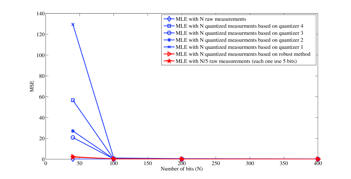
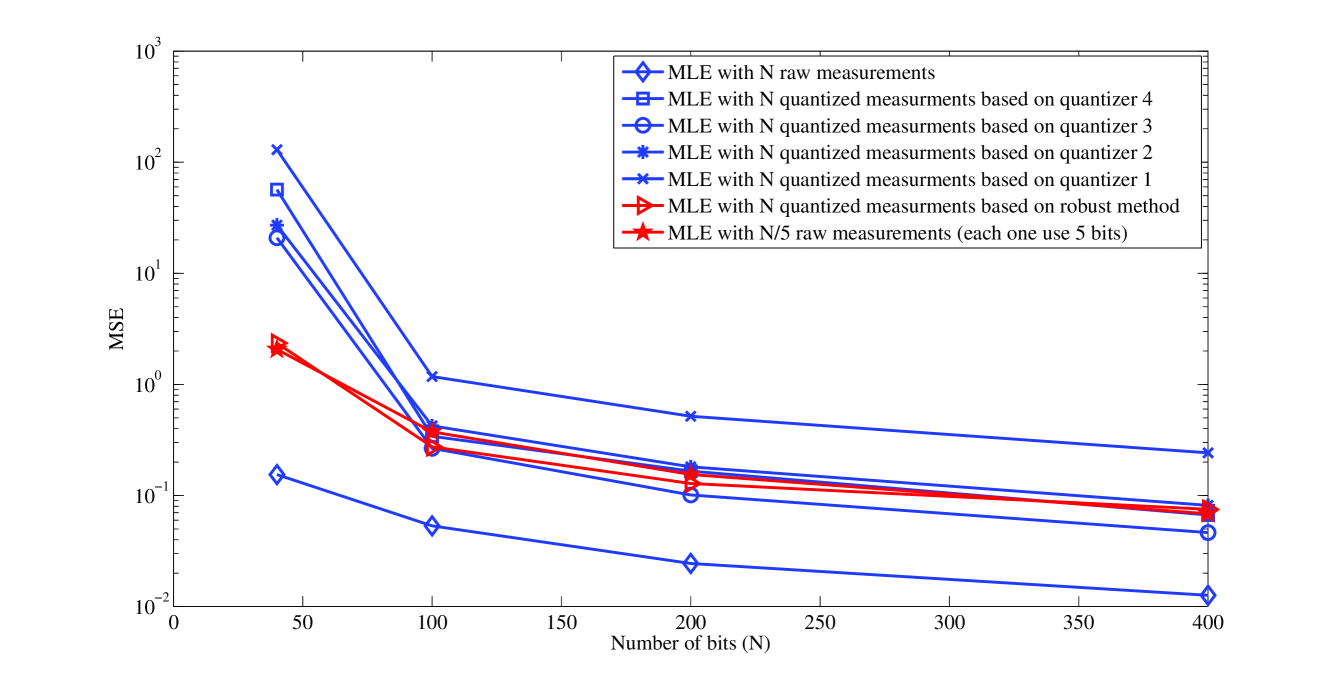
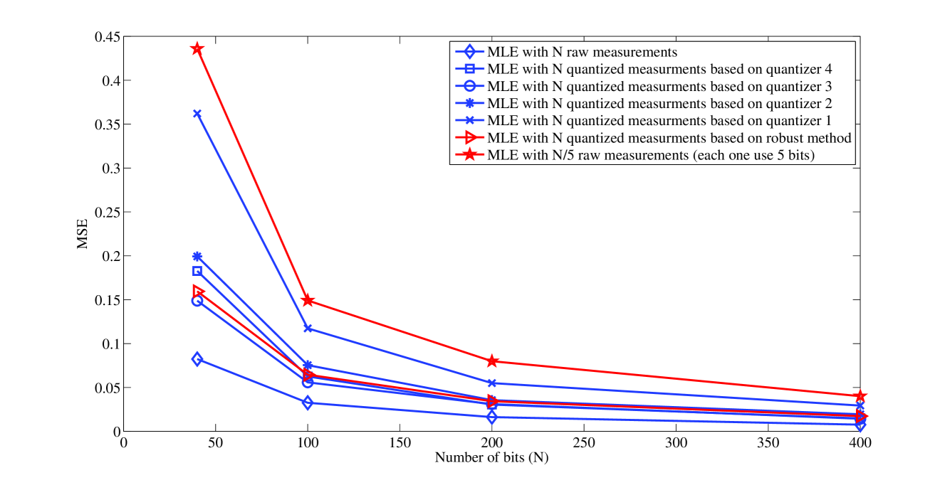
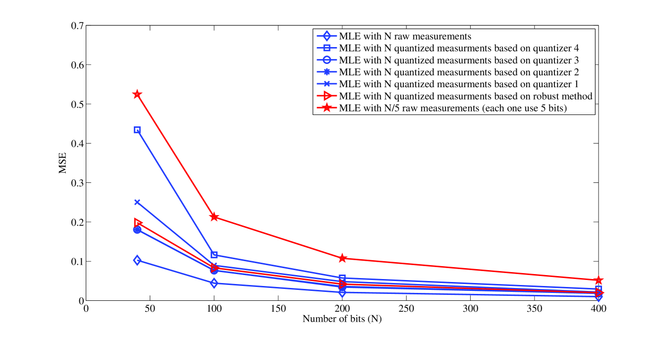
The robustness of the MLE with multiple quantizers is illustrated in Figs. 2–5. In Figs. 2–5, MSEs based on 1000 Monte Carlo (M.C.) runs as a function of the number of measurements $N=[40,100,200,400]$ for different estimation methods (MLE with single quantizer, robust MLE and MLE with raw measurements) are plotted for parameters $\theta_{0}=1.0759$, $\theta_{1}=4$ and $\theta_{2}=5$ respectively, where $\theta_{0}=1.0759$ corresponds to the dependence measure namely Spearman’s $\rho=0.5$. Figs 2–3 present the MSEs of $\theta_{0}$ in linear and logarithmic scales respectively. In Figs 4–5, we present the MSEs of $\theta_{1}$ and $\theta_{2}$ in linear scale respectively. In our work thus far, we have assumed that 1-bit quantized data is transmitted to the fusion center in simulations. We consider another system where finely quantized data (5-bit data corresponding to a subset of samples instead of 1-bit data corresponding to all the samples) is transmitted while maintaining the total number of bits equal to $N$. While evaluating the performance of the system with 5-bit data, we employ the results corresponding to raw data which, in fact, give more optimistic results. The MSEs based on 1000 M.C. runs of transmitting $N/5$ finely quantized 5-bit measurements are given in Figs 2–5 for $\theta_{0}$, $\theta_{1}$ and $\theta_{2}$ respectively.

From Figs 2–5, we have the following observations: (1). From Figs 2–5, MSEs based on 1000 M.C. runs for robust MLE are much smaller than those of the MLE based on the single quantizer that is the worst (outlier) in the group. This phenomenon is consistent with the results in Theorem 1 and Remark 1. Robust MLE is a conservative estimate, but it can avoid large errors in the worst case. The advantage of robustness (MSE of the worst MLE minus MSE of Robust MLE) is much larger than the loss due to conservative estimation to enhance robustness (MSE of Robust MLE minus MSE of the best one), especially in Figs 2, 3 and 4. (2). From Figs 2–3, a surprising result that is observed is that the Robust MLE based on 1000 M.C. runs has a significant advantage over MLE with a single quantizer, when the number of quantized measurements is small N=40. The reason is that, for small number of samples, the MLE with single quantizer is sensitive to the randomized samples so that it may be an outlier in each M.C. run resulting in poor performance. (3). By comparing our robust MLE with 1-bit quantized data with MLE that transmits a subset of finely quantized data in Figs 2–3, we observe that their performance of estimating $\theta_{0}$ is very close. However, for the performance of estimating $\theta_{1}$ and $\theta_{2}$, robust MLE is much better than the latter from Figures 4–5. Thus, robust MLE is a better estimation method in distributed dynamic systems with limited bandwidth.

5 Conclusion

In this paper, we have proposed an approach for robust distributed MLE with dependent quantized data under the assumption that the structure of the joint pdf is known, but it contains unknown deterministic parameters. We considered a practical estimation problem with a bivariate non-Gaussian pdf arising from the distributed constant false alarm rate (CFAR) detection systems. Simulation results show that the new MLE scheme is robust and much better than that based on the worst (outlier) quantization scheme from among the groups of quantizers. An important obersvation is that the robust MLE has a significant advantage over MLE with a single quantizer, when the number of quantized measurements is small.

Figure 2: MSEs of MLE of $\theta_{0}$ based on 1000 M.C. runs while using raw measurements, different quantizers and the robust MLE of $\theta_{0}$ for different number of measurements. Figure 2 is using linear scale.

Figure 3: Figure 2 using logarithmic scale.

Figure 4: MSEs of MLE of $\theta_{1}$ based on 1000 M.C. runs while using raw measurements, different quantizers and the robust MLE of $\theta_{1}$ for different number of measurements.

Figure 5: MSEs of MLE of $\theta_{2}$ based on 1000 M.C. runs while using raw measurements, different quantizers and the robust MLE of $\theta_{2}$ for different number of measurements.

References

- [1] George Casella and Roger L. Berger. Statistical Inference. Duxbury, New York, second edition, 2001.
- [2] Marco Casini, Andrea Garulli, and Antonio Vicino. Input design in worst-case system identification with quantized measurements. Automatica, 48:2997–3007, 2012.
- [3] Jun Fang and Hongbin Li. Distributed adaptive quantization for wireless sensor networks: From delta modulation to maximum likelihood. IEEE Transactions on Signal Processing, 56(10):5246–5257, 2008.
- [4] Jun Fang and Hongbin Li. Hyperplane-based vector quantization for distributed estimation in wireless sensor networks. IEEE Transactions on Information Theory, 55:5682–5699, 2009.
- [5] Boris I. Godoy, Graham C. Goodwin, Juan C. Aguero, Damian Marelli, and Torbjorn Wigren. On identification of fir systems having quantized output data. Automatica, 47:1905–1915, 2011.
- [6] Fredrik Gustafsson and Rickard Karlsson. Statistical results for system identification based on quantized observations. Automatica, 45:2794–2801, 2009.
- [7] Satish G. Iyengar, Pramod K. Varshney, and Thyagaraju Damarla. A parametric copula-based framework for hypothesis testing using heterogeneous data. IEEE Transactions on Signal Processing, 59(5):2308–2319, May 2011.
- [8] Dami n Marelli, Keyou You, and Minyue Fu. Identification of ARMA models using intermittent and quantized output observations. Automatica, 49:360–369, 2013.
- [9] V. Megalooikonomou and Y. Yesha. Quantizer design for distributed estimation with communication constraints and unknown observation statistics. IEEE Transactions on Communications, 48(2):181–184, February 2000.
- [10] R. B. Nelsen. An Introduction to Copulas. Springer-Verlag, New York, 1999.
- [11] A. Ribeiro and G. B. Giannakis. Bandwidth-constrained distributed estimation for wireless sensor networks–Part I: Gaussian case. IEEE Transactions on Signal Processing, 54(3):1131–1143, March 2005.
- [12] James C. Spall. Asymptotic normality and uncertainty bounds for reliability estimates from subsystem and full system tests. In American Control Conference, pages 56–61, Fairmont Queen Elizabeth, Montreal, Canada, June 2012.
- [13] Ashok Sundaresan and Pramod K. Varshney. Location estimation of a random signal source based on correlated sensor observations. IEEE Transactions on Signal Processing, 59(2):787–799, February 2011.
- [14] A. W. Van der Vaart. Asymptotic statistics. Cambridge University Press, New York, 2000.
- [15] Pramod K. Varshney. Distributed Detection and Data Fusion. New York: Springer-Verlag, 1997.
- [16] Venugopal V. Veeravalli and Pramod K. Varshney. Distributed inference in wireless sensor networks. Philosophical Transactions of the Royal Society A: Mathematical, Physical and Engineering Sciences, 370(1958):100–117, January 2012.
- [17] Le Yi Wang, G. George Yin, Ji-Feng Zhang, and Yanlong Zhao. System Identification with Quantized Observations. Birkhauser, 2010.
- [18] Torbjorn Wigren. Approximate gradients, convergence and positive realness in recursive identification of a class of non-linear systems. International Journal of Adaptive Control and Signal Processing, 9:325–354, 1995.
- [19] Jin-Jun Xiao, Alejandro Ribeiro, Zhi-Quan Luo, and Georgios B. Giannakis. Distributed compression-estimation using wireless sensor networks. IEEE Signal Processing Magazine, 23(4):27–41, July 2006.