Interstellar MHD Turbulence and Star Formation

Abstract

This chapter reviews the nature of turbulence in the Galactic interstellar medium (ISM) and its connections to the star formation (SF) process. The ISM is turbulent, magnetized, self-gravitating, and is subject to heating and cooling processes that control its thermodynamic behavior, causing it to behave approximately isobarically, in spite of spanning several orders of magnitude in density and temperature. The turbulence in the warm and hot ionized components of the ISM appears to be trans- or subsonic, and thus to behave nearly incompressibly. However, the neutral warm and cold components are highly compressible, as a consequence of both thermal instability (TI) in the atomic gas and of moderately-to-strongly supersonic motions in the roughly isothermal cold atomic and molecular components. Within this context, we discuss: i) the production and statistical distribution of turbulent density fluctuations in both isothermal and polytropic media; ii) the nature of the clumps produced by TI, noting that, contrary to classical ideas, they in general accrete mass from their environment in spite of exhibiting sharp discontinuities at their boundaries; iii) the density-magnetic field correlation (and, at low densities, lack thereof) in turbulent density fluctuations, as a consequence of the superposition of the different wave modes in the turbulent flow; iv) the evolution of the mass-to-magnetic flux ratio (MFR) in density fluctuations as they are built up by dynamic compressions; v) the formation of cold, dense clouds aided by TI, in both the hydrodynamic (HD) and the magnetohydrodynamic (MHD) cases; vi) the expectation that star-forming molecular clouds are likely to be undergoing global gravitational contraction, rather than being near equilibrium, as generally believed, and vii) the regulation of the star formation rate (SFR) in such gravitationally contracting clouds by stellar feedback which, rather than keeping the clouds from collapsing, evaporates and disperses them while they collapse.

1 Introduction

The interstellar medium (ISM) of our galaxy (the Milky Way, or simply, The Galaxy) is mixture of gas, dust, cosmic rays, and magnetic fields that occupy the volume in-between stars (e.g., Ferrière, 2001). The gasesous component, with a total mass $\sim 10^{10}M_{\odot}$, may be in either ionized, neutral atomic or neutral molecular forms, spanning a huge range of densities and temperatures, from the so-called hot ionized medium (HIM), with densities $n\sim 10^{-2}{\rm~{}cm}^{-3}$ and temperatures $T\sim 10^{6}$ K, through the warm ionized and neutral (atomic) media (WIM and WNM, respectively, both with $n\sim 0.3{\rm~{}cm}^{-3}$ and $T\sim 10^{4}$ K) and the cold neutral (atomic) medium (CNM, $n\sim 30{\rm~{}cm}^{-3}$, $T\sim 100$ K), to the giant molecular clouds (GMCs, $n\lower 2.15277pt\hbox{$\;\buildrel>\over{\sim}\;$}100{\rm~{}cm}^{-3}$ and $T\sim 10$–20 K). These span several tens of parsecs across, and, in turn, contain plenty of substructure, which is commonly classified into clouds ($n\sim 10^{3}{\rm~{}cm}^{-3}$, size scales $L$ of a few parsecs), clumps ($n\sim 10^{4}{\rm~{}cm}^{-3}$, $L\sim 1$ pc), and cores ($n\lower 2.15277pt\hbox{$\;\buildrel>\over{\sim}\;$}10^{5}{\rm~{}cm}^{-3}$, $L\sim 0.1$ pc). It is worth noting that the temperature of most molecular gas is remarkably uniform, $\sim 10$–30 K.

Moreover, the ISM is most certainly turbulent, as typical estimates of the Reynolds number ($R_{\rm e}$) within it are very large. For example, in the cold ISM, $R_{\rm e}\sim 10^{5}$–$10^{7}$ (Elmegreen & Scalo, 2004, §4.1). This is mostly due to the very large spatial scales involved in interstellar flows. Because the temperature of the ISM varies so much from one type of region to another, so does the sound speed, and therefore the turbulent velocity fluctuations are often moderately or even strongly supersonic (e.g., Heiles & Troland, 2003; Elmegreen & Scalo, 2004, and references therein). In these cases, the flow is significantly compressible, inducing large-amplitude (nonlinear) density fluctuations. The density enhancements thus formed constitute dense clouds and their substructure (e.g., Sasao, 1973; Elmegreen, 1993; Ballesteros-Paredes et al., 1999a).

In addition to being turbulent, the ISM is subject to a number of additional physical processes, such as gravitational forces exerted by the stellar and dark matter components as well as by its own self-gravity, magnetic fields, cooling by radiative microscopic processes, and radiative heating due both to nearby stellar sources as well as to diffuse background radiative fields. It is within this complex and dynamical medium that stars are formed by the gravitational collapse of certain gas parcels.

In this chapter, we focus on the interaction between turbulence, the effects of radiative heating and cooling, which effectively enhance the compressibility of the flow, the self-gravity of the gas, and magnetic fields. Their complex interactions have a direct effect on the star formation process. The plan of the chapter is as follows: in §2 we briefly recall the effects that the net heating and cooling have on the effective equation of state of the flow and, in the case of thermally unstable flows, on its tendency to spontaneously segregate in distinct phases. Next, in §3 we discuss a few basic notions about turbulence and the turbulent production of density fluctuations in both the hydrodynamic (HD) and magnetohydrodynamic cases, to then discuss, in §4, the evolution and properties of clouds and clumps formed by turbulence in multiphase media. In §5, we discuss the likely nature of turbulence in the diffuse (warm and hot) components of the ISM, as well as in the dense, cold atomic and molecular clouds, suggesting that in the latter, at least during the process of forming stars, the velocity field may be dominated by gravitational contraction. Next, in §6 we discuss the regulation of star-formation (SF) in gravitationally contracting molecular clouds (MCs), in particular whether it is accomplished by magnetic support, turbulence, or stellar feedback, and how. Finally, in §7 we conclude with a summary and some final remarks.

2 ISM Thermodynamics: Thermal Instability

The ISM extends essentially over the entire disk of the Galaxy and, when considering a certain dense subregion of it, such as a cloud or cloud complex, it is necessary to realize that any such subregion constitutes an open system, whose interactions with its environment need to be taken into account. A fundamental form of interaction with the surroundings, besides dynamical interactions, is through the exchange of heat, which occurs mostly through heating by the UV background radiation produced by distant massive stars, local heating when nearby stellar sources (OB star ionization heating and supernova explosions), cosmic ray heating, and cooling by thermal and line emission from dust and gas, respectively (see, e.g., Dalgarno & McCray, 1972; Wolfire et al., 1995).

Globally, and as a first approximation, the ISM is roughly isobaric, as illustrated in Fig. 1. As can be seen there, most types of regions, either dilute or dense, lie within an order of magnitude from a thermal pressure $P\sim 3000$ K${\rm~{}cm}^{-3}$. The largest deviations from this pressure uniformity are found in Hii regions, which are the ionized regions around massive stars due to their UV radiation output, and in molecular clouds, which, as we shall see in §5.5, are probably pressurized by gravitational compression.

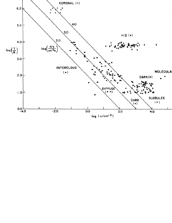
Figure 1: Thermal pressure in various types of interstellar regions. The points labeled coronal correspond essentially to what we refer to as the HIM in the text; intercloud regions refer to the WIM and WNM; diffuse, to CNM clouds, and dark, globule and molecular to molecular gas. From Myers (1978).

The peculiar thermodynamic behavior of the ISM is due to the functional forms of the radiative heating and cooling functions acting on it, which depend on the density, temperature, and chemical composition of the gas. The left panel of Fig. 2 shows the temperature dependence of the cooling function $\Lambda$ (Dalgarno & McCray, 1972). One well-known crucial consequence of this general form of the cooling is that the atomic medium is thermally unstable (Field, 1965) in the density range $1\lower 2.15277pt\hbox{$\;\buildrel<\over{\sim}\;$}n\lower 2.15277pt\hbox{$\;\buildrel<\over{\sim}\;$}10{\rm~{}cm}^{-3}$ (corresponding to $5000\lower 2.15277pt\hbox{$\;\buildrel>\over{\sim}\;$}T\lower 2.15277pt\hbox{$\;\buildrel>\over{\sim}\;$}30$ K), meaning that the medium tends to spontaneously segregate into two stable phases, one warm and diffuse, with $n\sim 0.3{\rm~{}cm}^{-3}$ and $T\sim 8000$ K, and the other cold and dense, with $n\sim 30{\rm~{}cm}^{-3}$ and $T\sim 80$ K, both at a pressure $P/k\sim 2500{~{}\rm K}{\rm~{}cm}^{-3}$ (Field et al., 1969; Wolfire et al., 1995, see also the reviews by Meerson 1996; Vázquez-Semadeni et al. 2003; Vázquez-Semadeni 2013), as illustrated in the right panel of Fig. 2. The cold gas is expected to form small clumps, since the fastest growing mode of the instability occurs at vanishingly small scales in the absence of thermal conductivity, or at scales $\sim 0.1$ pc for the estimated thermal conductivity of the ISM (see, e.g., Field, 1965; Audit & Hennebelle, 2005). Because the atomic gas in the ISM has two stable phases, it is often referred to as a thermally bistable medium.

It is important to note that, even if the medium is not thermally unstable, the balance between heating and cooling implies a certain functional dependence of $P_{\rm eq}(\rho)$, which is often approximated by a polytropic law of the form $P_{\rm eq}\propto\rho^{\gamma_{\rm e}}$ (e.g., Elmegreen, 1991; Vázquez-Semadeni et al., 1996), where ${\gamma_{\rm e}}$ is the effective polytropic exponent. In general, ${\gamma_{\rm e}}$ is not the ratio of specific heats for the gas in this case, but rather a free parameter that depends on the functional forms of $\Lambda$ and $\Gamma$. The isobaric mode of thermal instability (TI) corresponds to ${\gamma_{\rm e}}<0$. A flow is sometimes said to be softer as the parameter ${\gamma_{\rm e}}$ becomes smaller.

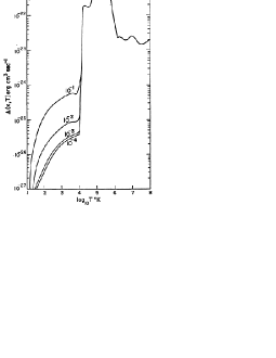
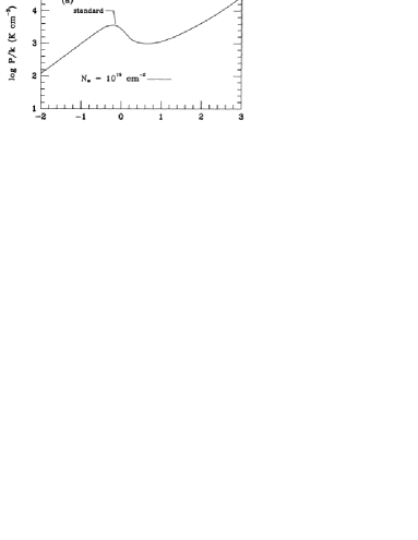
Figure 2: Left: Temperature dependence of the cooling function $\Lambda$. The labels indicate values of the ionization fraction (per number) of the gas. From Dalgarno & McCray (1972). Right: Thermal-equilibrium pressure $P_{\rm eq}$ as a function of number density for “standard” conditions of metallicity and background UV radiation for the atomic medium. The horizontal axis gives $\log_{10}(n/{\rm cm}^{3})$. From Wolfire et al. (1995).

3 Compressible Polytropic MHD Turbulence

3.1 Equations

In the previous section we have discussed thermal aspects of the ISM, whose main dynamical effect is the segregation of the medium into the cold and warm phases. Let us now discuss dynamics. As was mentioned in §1, the ISM is in general turbulent and magnetized, and therefore it is necessary to understand the interplay between turbulence, magnetic fields, and the effects of the net cooling ($n\Lambda-\Gamma$), which affects the compressibility of the gas (Vázquez-Semadeni et al., 1996).

The dynamics of the ISM are governed by the fluid equations, complemented by self-gravity, the heating and cooling terms in the energy equation, and the equation of magnetic flux conservation (e.g., Shu, 1992):

$$\frac{\partial\rho}{\partial t}+{\bf u}\cdot\nabla\rho = -\rho\nabla\cdot{\bf u},$$ (1)

$$\frac{\partial{\bf u}}{\partial t}+{\bf u}\cdot\nabla{\bf u} = -\frac{\nabla P}{\rho}-\nabla\varphi+\nu\left[\nabla^{2}{\bf u}+\frac{\nabla(\nabla\cdot{\bf u})}{3}\right]+\frac{1}{4\pi\rho}\bigl{(}\nabla\times{{\bf B}}\bigr{)}\times{{\bf B}},$$ (2)

$$\frac{\partial e}{\partial t}+{\bf u}\cdot\nabla e = -(\gamma-1)e\nabla\cdot{\bf u}+\Gamma-n\Lambda,$$ (3)

$$\frac{\partial{\vec{B}}}{\partial t}+\nabla\times(\vec{B}\times{\bf u}) = -\nabla\times(\eta\nabla\times{\bf B})+\nabla\times\left\{\frac{{\bf B}}{4\pi{\gamma_{\rm c}}\rho_{\rm n}\rho_{\rm i}}\times\left[{\bf B}\times\left(\nabla\times{\bf B}\right)\right]\right\},$$ (4)

$$\nabla^{2}\varphi = 4\pi G\rho,$$ (5)

where $\rho=\mu_{\rm m}m_{\rm H}n$ is the mass density, $\mu_{\rm m}$ is the mean particle mass, $m_{\rm H}$ is the hydrogen mass, ${\bf u}$ is the velocity vector, $e$ is the internal energy per unit mass, ${\bf B}$ is the magnetic field strength vector, $\varphi$ is the gravitational potential, $\nu$ is the kinematic viscosity, $\eta$ is the electrical resistivity, and ${\gamma_{\rm c}}$ is the collisional coupling constant between neutrals and ions in a partially ionized medium. Equation (1) represents mass conservation, and is also known as the continuity equation. Equation (2) is the momentum conservation, or Navier-Stokes equation per unit mass, with additional source terms representing the gravitational force $\nabla\varphi/\rho$ and the Lorentz force. In turn, the gravitational potential is given by Poisson’s equation, eq. (5). Equation (3) represents the conservation of internal energy, with $\Gamma$ being the heating function and $\Lambda$ the cooling function. The combination $n\Lambda-\Gamma$ is usually referred to as the net cooling, and the condition $n\Lambda=\Gamma$ is known as the thermal equilibrium condition. Finally, eq. (4) represents the conservation of magnetic flux (see below). Equations (1)–(5) are to be solved simultaneously, given some initial and boundary conditions.

A brief discussion of the various terms in the momentum and flux conservation equations is in order. In eq. (2), the second term on the left is known as the advective term, and represents the transport of $i$-momentum by the $j$ component of the velocity, where $i$ and $j$ represent any two components of the velocity. It is responsible for mixing. The pressure gradient term (first term on the right-hand side [RHS]) in general acts to counteract pressure, and therefore density, gradients across the flow. The term in the brackets on the RHS, the viscous term, being of a diffusive nature, tends to erase velocity gradients, thus tending to produce a uniform flow. Finally, the last term on the RHS is the Lorentz force.

On the other hand, eq. (4), assuming $\eta=0$ (i.e., zero electrical resistivity, or equivalently, infinite conductivity) and ${\gamma_{\rm c}}\rightarrow\infty$ (i.e., perfect coupling between neutrals and ions), implies that the magnetic flux $\Phi$ through a Lagrangian cross-sectional area $A$, given by

$$\Phi\equiv\int_{A}{\bf B}\cdot\hat{\vec{n}}~{}\mathrm{d}A,$$ (6)

remains constant in time as the area moves with the flow. This is the property known as flux freezing, and implies that the gas can slide freely along field lines, but drags the field lines with it when it moves perpendicularly to them. Note that this condition is often over-interpreted as to imply that the magnetic and the density fields must be correlated, but this is an erroneous notion. Only motions perpendicular to the magnetic field lines produce a correlation between the two fields, while motions parallel to the lines leave the magnetic field unaffected, while the density field can fluctuate freely. We discuss this at more length in §3.4.

The first term on the RHS of eq. (4) represents dissipation of the magnetic flux by electrical resistivity, and gives rise to the phenomenon of reconnection of field lines (see, e.g., the book by Shu 1992, and the review by Lazarian 2012). The second term on the RHS of eq. (4) represents ambipolar diffusion (AD), the deviation from the perfect flux-freezing condition that occurs for the neutral particles in the flow due to their slippage with respect to the ions in a partially ionized medium. We will further discuss the role of AD in the process of star formation (SF) in §§3.4 and 5.5.

3.2 Governing Non-Dimensional Parameters

Turbulence develops in a flow when the ratio of the advective term to the viscous term becomes very large. That is,

$$\frac{{\cal O}\left[{\bf u}\cdot\nabla{\bf u}\right]}{{\cal O}\left[\nu\left(\nabla^{2}{\bf u}+\frac{\nabla(\nabla\cdot{\bf u})}{3}\right)\right]}\sim\frac{U^{2}}{L}\left[\nu\frac{U}{L^{2}}\right]^{-1}\sim\frac{UL}{\nu}\equiv R_{\rm e}\gg 1,$$ (7)

where $R_{\rm e}$ is the Reynolds number, $U$ and $L$ are characteristic velocity and length scales for the flow, and ${\cal O}$ denotes “order of magnitude”. This condition implies that the mixing action of the advective term overwhelms the velocity-smoothing action of the viscous term.

On the other hand, noting that the advective and pressure gradient terms contribute comparably to the production of density fluctuations, we can write

$$1\sim\frac{{\cal O}\left({\bf u}\cdot\nabla{\bf u}\right)}{{\cal O}\left(\nabla P/\rho\right)}\sim\frac{U^{2}}{L}\left[\frac{\Delta P}{L\rho}\right]^{-1} \sim U^{2}\left(\frac{c_{\rm s}^{2}\Delta\rho}{\rho}\right)^{-1}\equiv M_{\rm s}^{2}\left(\frac{\Delta\rho}{\rho}\right)^{-1},$$ (8)

$$\Rightarrow\frac{\Delta\rho}{\rho} \sim M_{\rm s}^{2},$$ (9)

where $M_{\rm s}\equiv U/c_{\rm s}$ is the sonic Mach number, $\Delta\rho/\rho$ is the density jump, and we have made the approximation that $\Delta P/\Delta\rho\sim c_{\rm s}^{2}$, where $c_{\rm s}$ is the sound speed. Equation (9) then implies that strong compressibility requires $M_{\rm s}\gg 1$. Conversely, flows with $M_{\rm s}\ll 1$ behave incompressibly, even if they are gaseous. Such is the case, for example, of the Earth’s atmosphere. In the incompressible limit, $\rho=$ cst., and thus eq. (1) reduces to $\nabla\cdot{\bf u}=0$. Note, however, that the requirement $M_{\rm s}\gg 1$ for strong compressibility applies for flows that behave nearly isothermally, for which the approximation $\Delta P/\Delta\rho\sim c_{\rm s}^{2}$ is valid, while “softer” (cf. §2) flows have much larger density jumps at a given Mach number. For example, Vázquez-Semadeni et al. (1996) showed that polytropic flows of the form $P\propto\rho^{\gamma_{\rm e}}$ with ${\gamma_{\rm e}}\rightarrow 0$, have density jumps of the order $e^{M_{\rm s}^{2}}$.

A trivial, but often overlooked, fact is that, in order to produce a density enhancement in a certain region of the flow, the velocity at that point must have a negative divergence (i.e., a convergence), as can be seen by rewriting eq. (1) as

$$\frac{\mathrm{d}\rho}{\mathrm{d}t}=-\rho\nabla\cdot{\bf u},$$ (10)

where $\mathrm{d}/\mathrm{d}t\equiv\partial/\partial t+{\bf u}\cdot\nabla$ is the total, material, or Lagrangian derivative. However, it is quite common to encounter in the literature discussions of pre-existing density enhancements (“clumps”) in hydrostatic equilibrium. It should be kept in mind that these can only exist in multi-phase media, where a dilute, warm phase can have the same pressure as a denser, but colder, clump. But even in this case, the formation of that clump must have initially involved the convergence of the flow towards the cloud, and the hydrostatic situation is applicable in the limit of very long times after the formation of the clump, when the convergence of the flow has subsided.

Finally, two other important parameters determining the properties of a magnetized flow are the Alfvénic Mach number, $M_{\rm A}\equiv U/\upsilon_{\rm A}$ and the plasma beta, $\beta\equiv P_{\rm th}/P_{\rm mag}$ where $\upsilon_{\rm A}=B/\sqrt{4\pi\rho}$ is the Alfvén speed. Similarly to the non-magnetic case, large values of the Alfvénic Mach number are required in order to produce significant density fluctuations through compressions perpendicular to the magnetic field. However, it is important to note, as mentioned in §3.1, that compressions along the magnetic field lines are not opposed at all by magnetic forces. Note that, in the isothermal case, $\beta=2c_{\rm s}^{2}/\upsilon_{\rm A}^{2}$.

3.3 Production of Density Fluctuations. The Non-Magnetic Case

As mentioned in the previous sections, strongly supersonic motions, or the ability to cool rapidly, allow the production of large-amplitude density fluctuations in the flow. Note, however, that the nature of turbulent density fluctuations in a single-phase medium (such as, for example, a regular isothermal or adiabatic flow) is very different from that of the cloudlets formed by TI (cf. §2). In a single-phase turbulent medium, turbulent density fluctuations must be transient, because in this case a higher density generally implies a higher pressure, and therefore the fluctuations must re-expand (in roughly a sound-crossing time) after the compression that produced them has subsided.

Note that the above result includes the case with self-gravity, since in single-phase media, although hydrostatic equilibrium solutions do exist, they are generally unstable. Specifically, the singular isothermal sphere is known to be unstable (Shu, 1977), and non-singular configurations such as the Bonnor-Ebert (BE) spheres (Ebert, 1955; Bonnor, 1956) need to be truncated so that the central-to-peripheral density ratio is smaller than a critical value $\sim 14$ in order to be stable. Such stable configurations, however, need to be confined by some means to prevent their expansion. Generally, the confining agent is assumed to consist of a dilute, warm phase that provides pressure without adding additional weight. However, such a warm phase is not available in single-phase flows, and the only way to confine the BE sphere is to continuously extend it to infinity, in which case the central-to-peripheral density ratio also tends to infinity, and the configuration is unstable (Vázquez-Semadeni et al., 2005a).

Instead, in multiphase flows, abrupt density variations may exist between different phases even though they may be at roughly the same thermal pressure, and therefore, the dense clumps do not tend to re-expand. In the remainder of this section we discuss the probability distribution of the density fluctuations, the nature of the resulting clumps and their interfaces with their environment, the correlation between the magnetic and density fields, and the evolution of the mass-to-magnetic flux ratio as the clumps are assembled by turbulent compressions.

The Probability Distribution of Density Fluctuations. The Non-Magnetic Case

For astrophysical purposes it is important to determine the distribution of the density fluctuations, as they may constitute, or at least provide the seeds for, what we normally refer to as “clouds” in the ISM. In single-phase media, however, due to the transient nature of turbulent density fluctuations, this distribution refers to a time-stationary population of fluctuations, even though the fluctuations themselves will appear and disappear on timescales of the order of their crossing time at the speed of the velocity fluctuations that produce them.

The probability density function (PDF) of the density field in turbulent isothermal flows was initially investigated through numerical simulations. Vázquez-Semadeni (1994) found that, in the isothermal case, the PDF posesses a lognormal form. A theory for the emergence of this functional form was later proposed by Passot & Vázquez-Semadeni (1998), in which the production of density fluctuations was assumed to arise from a succession of random compressive or expansive waves, each one acting on the value of the density left by the previous one. The amplitude of each wave can then be described as a random variable, characterized by some probability distribution. Because the medium contains a unique distribution of (compressible) velocity fluctuations, and because the density jumps in isothermal flow depend only on Mach number but not on the local density, the density fluctuations belong all to a unique distribution as well, yet each one can be considered independent of the others if the global time scales considered are much longer than the autocorrelation time of the velocity divergence (Blaisdell et al., 1993). Finally, because the density jumps are multiplicative in the density (cf. eq. 9), then they are additive in $s\equiv\ln\rho$. Under these conditions, the Central Limit Theorem can be invoked for the increments in $s$, implying that $s$ will be normally distributed, independently of the distribution of the waves. In consequence, $\rho$ will have a lognormal PDF.

In addition, Passot & Vázquez-Semadeni (1998) also argued that the variance of the density fluctuations should scale linearly with $M_{\rm s}$, a suggestion that has been investigated further by other groups (Padoan et al., 1997; Federrath et al., 2008). In particular, using numerical simulations of compressible turbulence driven by either solenoidal (or “vortical”) or compressible (or “potential”) forces, the latter authors proposed that the variance of $s$ is given by

$$\sigma_{s}=\ln(1+bM_{\rm s}^{2}),$$ (11)

where $b$ is a constant whose value depends on the nature of the forcing, taking the extreme values of $b=1/3$ for purely solenoidal forcing, and $b=1$ for purely compressible forcing. The lognormal density PDF for the one-dimensional, isothermal simulations of Passot & Vázquez-Semadeni (1998), with its dependence on $M_{\rm s}$, is illustrated in the left panel of Fig. 3.

Figure 3: Left: Lognormal density PDFs for isothermal one-dimensional simulations at various Mach numbers, indicated by the labels. The independent variable is $s\equiv\ln\rho$. Right: Density PDFs for polytropic cases (i.e., with $P\propto\rho^{{\gamma_{\rm e}}}$), with effective polytropic exponent ${\gamma_{\rm e}}=0.3$ (top) and ${\gamma_{\rm e}}=1.7$ (bottom). From Passot & Vázquez-Semadeni (1998).

Figure 4: Plots of $s=\ln\rho$ of the density field in one-dimensional simulations of polytropic flows with a resolution of 6144 grid points by Passot & Vázquez-Semadeni (1998). Top: A simulation with ${\gamma_{\rm e}}=0.5$, exhibiting high-amplitude, narrow density peaks, due to the low sound speed at high density. Bottom: A simulation with ${\gamma_{\rm e}}=1.5$, exhibiting low-amplitude, extended density peaks and deep “voids” due to the high values of the sound speed at high densities, and low values at low densities.

Finally, Passot & Vázquez-Semadeni (1998, see also Padoan & Nordlund 1999) also investigated the case where the flow behaves as a polytrope (cf. §2) with arbitrary values of ${\gamma_{\rm e}}$, by noting that in this case the sound speed is not constant, but rather depends on the density as $c_{\rm s}\propto\rho^{({\gamma_{\rm e}}-1)/2}$, implying that the local Mach number of a fluid parcel now depends on the local density besides its dependence on the value of the flow velocity. Introducing this dependence of $M_{\rm s}$ on $\rho$ in the expression for the lognormal PDF, Passot & Vázquez-Semadeni (1998) concluded that the density PDF should develop a power-law tail, at high densities when ${\gamma_{\rm e}}<1$, and at low densities when ${\gamma_{\rm e}}>1$. This result was then confirmed by numerical simulations of polytropic turbulent flows (Fig. 3, right panel). Physically, the cause for the deviation of the PDF from the lognormal shape is that, for ${\gamma_{\rm e}}>1$, the sound speed increases with increasing density, and therefore, high-density regions can re-expand and disappear quickly, while “voids”, with a lower sound speed, last for long times. For ${\gamma_{\rm e}}<1$, the sound speed decreases for increasing density, and the behavior is reversed: large-amplitude density peaks have lower sound speeds and therefore last for longer times, while the voids have higher sound speeds and disappear quickly. The resulting topology of the density field is illustrated in the one-dimensional case in Fig. 4.

The Nature of Turbulent Clumps

The Ambiguity of Clump Boundaries and Masses

The clumps produced as turbulent density fluctuations are precisely that: fluctuations in a continuum. Besides, there is in general a mass and energy flux through any fixed boundary we choose to define around the local density maximum (Ballesteros-Paredes et al., 1999a). This is especially true in isothermal flows, where no transition from a diffuse phase to a dense one with the same pressure can occur, so that the only density discontinuities possible are those produced by shocks. In this case, the density fluctuations produced by turbulent compressions (a transient event of elevated ram pressure) must always be transients, and must eventually re-expand or collapse (see §3.3). In thermally bistable media, the “boundaries” are somewhat better defined, although there is still mass flux through them (see §4.2).

The elusiveness of the notion of clump boundaries implies that we must rethink some of our dearest notions about clumps. First of all, the mass of a cloud or clump is not well defined, and additionally must evolve in time. It is ill-defined because the clump boundary itself is. Several procedures exist for “extracting” clumps from observational maps or from numerical simulations. One of the most widely employed algorithms for locating clumps is Clumpfind (Williams et al., 1994), which works by locating local peaks in the field being examined and then following the field down its gradient until another clump profile is met, at which point an arbitrary boundary is defined between the two. However, this procedure, by construction, is uncapable of recognizing “hierarchical”, or “nested”, structures, where one coherent “parent” clump contains other equally coherent “child” ones. Moreover, not surprisingly, it has been shown that the clump sets obtained from application of this algorithm depend sensitively on the parameters chosen for the definition of the clumps (Pineda et al., 2009). Conversely, a technique that, by definition, is capable of detecting “parent” structures, is based on “structure trees”, or “dendrograms” (e.g., Houlahan & Scalo, 1992; Rosolowsky et al., 2008), which works by thresholding an image at successive intensity levels, and following the “parent”-“child” relationship between the structures identified at the different levels. Clearly, the two techiques applied to the same data produce very different sets of clumps and, in consequence, different clump mass distributions.

This variety of procedures for defining clumps illustrates the ambiguity inherent in defining a finite object that is actually part of a continuum, and implies that the very concept of the mass of a clump carries with it a certain level of inherent uncertainty.

Clump masses evolve in time

A turbulent density fluctuation is a local density enhancement produced by a velocity field that at some moment in time is locally convergent, as indicated by eq. (10). This process accumulates mass in a certain region of space (“the clump”), with the natural consequence that the mass of the clump must increase with time, at least initially, if the clump is defined, for example, as a connected object with density above a certain threshold. This definition corresponds, for example, to clumps defined as compact objects observed in a particular molecular tracer, since such tracers require the density to be above a certain threshold to be excited.

The growth of the clump’s density (and mass) lasts as long as the total pressure within the clump (which may include thermal, turbulent and magnetic components) is smaller than the ram pressure from the compression. However, in a single-phase medium, once the turbulent compression subsides, the clump, which is at higher density than its surroundings, and therefore also at a higher pressure, must therefore begin to re-expand, unless it manages to become gravitationally unstable and proceed to collapse (Vázquez-Semadeni et al., 2005a; Gómez et al., 2007, see also §3.3). Therefore, the mass above the clump-defining density threshold may begin to decrease again. (Again, see §4.2 for the case of clumps forming in multi-phase media.) As we shall see in §3.4, the fact that clumps’ masses evolve in time has direct implications for the amount of magnetic support that the clump may have against its self-gravity.

3.4 Production of Density Fluctuations. The Magnetic Case.

In the magnetized case, the problem of density fluctuation production becomes more complex, as the turbulent velocity field also produces magnetic field fluctuations. In this section, we discuss two problems of interest in relation to SF: The correlation of the density and magnetic fluctuations, and the effect of the magnetic field on the PDF of density fluctuations.

Density-Magnetic Field Correlation

This is a highly relevant issue in relation to SF, as the “standard” model of magnetically-regulated SF (hereafter SMSF; see, e.g., the reviews by Shu et al., 1987; Mouschovias, 1991) predicted that magnetic fields should provide support for the density fluctuations (“clumps”) against their self-gravity, preventing collapse, except for the material that, through AD, managed to lose its support (see the discussion in §5.5). Thus, the strength of the magnetic field induced in the turbulent density fluctuations is an important quantity to determine.

Under perfect field-freezing conditions, the simplest scenario of a fixed-mass clump threaded by an initially uniform magnetic field, and undergoing an isotropic gravitational contraction implies that the field should scale as $B\propto\rho^{2/3}$ (Mestel, 1966), since the density scales as $\rho\propto R^{-3}$, where $R$ is the radius of the clump, while the flux-freezing condition implies that $B\propto R^{-2}$. The assumption that the clump is instead oblate, or disk-like, with the magnetic field providing support in the radial direction and thermal pressure providing support in the direction perpendicular to its plane, gives the scaling $B\propto\rho^{-1/2}$ (Mouschovias, 1976, 1991)

In a turbulent flow, however, the situation becomes more complicated. “Clumps” are not fixed-mass entities, but rather part of a continuum that possesses random, chaotic motions. In principle, unless the magnetic energy is much larger than the turbulent kinetic energy, the compressive motions that form a clump can have any orientation with respect to the local magnetic field lines, and thus the resulting density enhancement may or may not be accompanied by a corresponding magnetic field enhancement (cf. §3.1). In particular, Passot & Vázquez-Semadeni (2003, hereafter, PV03) studied this problem analytically in the isothermal case, by decomposing the flow into nonlinear, so-called “simple” waves (e.g., Landau & Lifshitz, 1959), which are the nonlinear extensions of the well known linear MHD waves (e.g., Shu, 1992), having the same three well-known modes: fast, slow, and Alfvén (Mann, 1995). For illustrative purposes, note that compressions along the magnetic field lines are one instance of the slow mode, while compressions perpendicular to the field lines (i.e., magnetosonic waves) are an instance of the fast mode. As is well known, Alfvén waves are transverse waves propagating along field lines, and carry no density enhancement. However, they can exert pressure, and the dependence of this pressure on the density has been investigated by McKee & Zweibel (1995) and PV03.

For simplicity and insight, PV03 considered the so-called “1+2/3-dimensional” case, also known as “slab geometry”, meaning that all three components of vector quantities are considered, but their variation is studied with respect to only one spatial dimension. For the Alfvén waves, they performed a linear perturbation analysis of a circularly polarized wave. They concluded that each of the modes is characterized by a different scaling between the magnetic pressure ($\propto B^{2}$) and the density, as follows:

$$B^{2} \propto c_{1}-\beta\rho$$      slow, (12)

$$B^{2} \propto\rho^{2}$$      fast, (13)

$$B^{2} \propto\rho^{{\gamma_{\rm m}}}$$      Alfvén, (14)

where $c_{1}$ is a constant, and ${\gamma_{\rm m}}$ is a parameter that can take values in the range (1/2,2) depending on the Alfvénic Mach number (see also McKee & Zweibel, 1995). Note that eq. (12) implies that for $\rho>c_{1}/\beta$ the slow mode disappears (Mann, 1995), so that only the fast and Alfvén modes remain. Conversely, note that, at low density, the magnetic pressure due to the fast and Alfvén modes becomes negligible in comparison with that due to the slow mode, which approaches a constant. This implies that a log-log plot of $B$ vs. $\rho$ will exhibit an essentially constant value of $B$ at very small values of the density. In other words, at low values of the density, the domination of the slow mode implies that the magnetic field exhibits essentially no correlation with the density.

PV03 were able to test these results numerically by taking advantage of the slab geometry, which allowed to set up waves propagating at well-defined angles with respect to the mean magnetic field, and therefore being able to isolate, or nearly isolate, the three different wave modes. The left panel of Fig. 5 shows the distribution of points in the $B^{2}$-$s$ space for a simulation dominated by the slow mode, exhibiting the behavior outlined above, corresponding to eq. (12). In contrast, the right panel of Fig. 5 shows the distribution of points in the same space for a simulation dominated by the fast mode, exhibiting the behavior indicated by eq. (13).

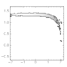
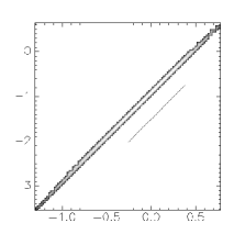
Figure 5: Two-dimensional histograms of the grid cells in numerical simulations in the $\ln B^{2}$ (vertical axis)-$\ln\rho$(horizontal axis) space. The gray scale indicates the density of points in this space. Left: A slab-geometry numerical simulation by PV03 dominated by the slow mode, exhibiting the behavior indicated by eq. (12). Right: Same as the left panel, but for a numerical simulation dominated by the fast mode, exhibiting the behavior indicated by eq. (13).

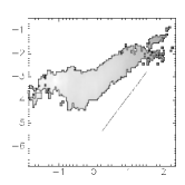
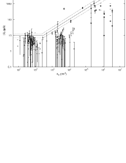
Figure 6: Left: Two-dimensional histogram of the grid cells in the $B^{2}$-$n$ space from a numerical simulation by PV03 in which both the slow and the fast modes are active. At low densities, the slow mode causes a density-independent magnetic field strength, while at higher densities, the fast mode produces a positive correlation. The straight-line segment has a slope of 2. Right: Magnetic field strength determinations by Zeeman splitting observations in molecular clouds, as compiled by Crutcher et al. (2010). The rising straight line segment has a slope $\approx 0.65$, implying $B^{2}\propto n^{1.3}$, in qualitative agreement with the numerical result.

The most important conclusion from eqs. (12)–(14) is that Now, in a turbulent flow in which all modes are active, the net, average scaling of the magnetic field with the density will arise from the combined effect of the various modes. Moreover, since at low densities the values of $B$ produced by the fast and Alfvén modes are also small, while the field strengths produced by the slow mode remain roughly constant, the field fluctuations will be dominated by the latter mode at low densities, and a roughly density-independent field strength is expected. Conversely, at high densities, the slow mode disappears, while the contribution from the fast and Alfvén modes will dominate, producing a field strength that increases with increasing density. Finally, because each mode produces a different dependence of the magnetic field strength with the density, we expect that the instantaneous value of the density at a certain location in physical space is not enough to determine the value of the magnetic field strength there. Instead, this value depends on the history of modes of the nonlinear waves that have passed through that location, naturally implying that, within a large cloud, a large scatter in the measured values of the magnetic field is expected. The expected net scaling of the field strength with the density is illustrated in the left panel of Fig. 6. These results are in qualitative agreement with detailed statistical analyses of the magnetic field distribution in the ISM (Crutcher et al., 2010), as illustrated in the right panel of Fig. 6.

Effect of the Magnetic Field on the Density PDF

According to the discussion in §3.3, the dependence of the pressure on density determines the shape of the density PDF, being a lognormal for the isothermal case, ${\gamma_{\rm e}}=1$. In the presence of a magnetic field, it would be natural to expect that the magnetic pressure, which in general does not need to behave as an isothermal polytrope, might cause deviations from the lognormal density PDF associated to isothermal turbulent flows.

However, the discussion above on the density-magnetic field correlation (or rather, lack thereof), implies that the magnetic pressure does not have a systematic effect on density fluctuations of a given amplitude, as the value of the magnetic field is not uniquely determined by the local value of the density. PV03 concluded that the effect of the magnetic pressure was more akin to a random forcing in the turbulent flow than to a systematic pressure gradient that opposes compression. As a consequence, the underlying density PDF determined by the functional form of the thermal pressure did not appear to be significantly affected by the presence of the magnetic field, except under very special geometrical setups in slab geometry, and that in fact are unlikely to persist in a more general three-dimensional setup. The persistence of the underlying PDF dictated by the thermodynamics in the presence of the magnetic field is in agreement with numerical studies of isothermal MHD turbulent flows that indeed have found approximately lognormal PDFs in isothermal flows (e.g., Padoan & Nordlund, 1999; Ostriker et al., 1999, 2001; Vázquez-Semadeni & García, 2001; Beresnyak et al., 2005), and bimodal density PDFs in thermally-bistable flows (Gazol et al., 2009), which we discuss in §4.1.

Evolution of the Mass-to-Magnetic Flux Ratio

The discussion in §3.3 implies that the mass deposited in a clump by turbulent compressions is a somewhat ill-defined quantity, depending on where and how one chooses to define the “boundaries” of the clump, and on the fact that its mass is time-dependent. This has important implications for the so-called mass-to-flux ratio (MFR) of the clump, and therefore, for the ability of the magnetic field to support the clump against its self-gravity.

As is well known (Mestel & Spitzer, 1956), a virial balance analysis implies that, for a cloud of mass $M$ threaded by a uniform field $B$, gravitational collapse can only occur if its MFR satisfies

$$\frac{M}{\Phi}>\left(\frac{M}{\Phi}\right)_{\rm crit}\equiv\left(\alpha\pi^{2}G\right)^{-1/2},$$ (15)

where $\alpha$ is a constant of order unity whose precise value depends on the shape and mass distribution in the cloud (see, e.g., Mestel & Spitzer, 1956; Nakano & Nakamura, 1978; Shu, 1992). Otherwise, the cloud is absolutely supported by the magnetic field, meaning that the support holds irrespective of the density of the cloud. In what follows, we shall denote the MFR, normalized to this critical value, by $\lambda$. Regions with $\lambda>1$ are called magnetically supercritical, while those with $\lambda<1$ are termed magnetically subcritical. Traditionally, it has been assumed that the mass of the cloud is well defined. However, our discussions above (§3.3) suggest that it may be convenient to revisit these notions.

When considering density enhancements (“cores”) formed by turbulent compressions within a cloud of size $L$, it is convenient to assume that the initial condition for the cloud is one with uniform density and magnetic field, and that the turbulence produces local fluctuations in the density and the magnetic field strength. A simple argument advanced by Vázquez-Semadeni et al. (2005a) then shows that the MFR of a core of size $\ell$ and MFR $\lambda_{\ell}$, must be within the range

$$\lambda_{0}\frac{\ell}{L}<\lambda_{\ell}<\lambda_{0},$$ (16)

where $\lambda_{0}$ is the MFR of the whole cloud. The lower limit applies for the case when the “core” is actually simply a subregion of the whole cloud of size $L$, with the same density and magnetic field strength. Since the density and field strength are the same, the mass of the core simply scales as $(\ell/L)^{3}$, while the magnetic flux scales as $(\ell/L)^{2}$. Therefore, the MFR of a subregion of size $\ell$ scales as $(\ell/L)$. Of course, this lower-limit extreme, corresponding to the case of a “core” of the same density and field strength as the whole cloud, is an idealization, since observationally such a structure cannot be distinguished from its parent cloud. Nevertheless, as soon as some compression has taken place, the core will be observationally distinguishable from the cloud (for example, by using a tracer that is only excited at the core’s density), and the measurement of the MFR in the core will be bounded from below by this limit.

On the other hand, the upper limit corresponds simply to the case where the entire cloud of size $L$ has been compressed isotropically to a size $\ell$, since in this case both the mass and the magnetic flux are conserved, and so is the MFR.

This reasoning has the implication that the MFR that is measured in a core within a cloud must be smaller than that measured for the whole cloud, as long as the condition of flux-freezing holds. Note that one could argue that this is only an observational artifact, and that the physically relevant mass is that associated to the whole flux tube the core belongs to, but this is only reflecting the ambiguity discussed above concerning the masses of clumps. In practice, the physically relevant mass for the computation of the MFR is the one responsible for the local gravitational potential well against which the magnetic field is providing the support, and this mass is precisely the mass of the core, not the mass along the entire flux tube, especially when phase transitions are involved.

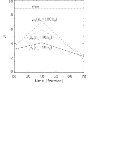
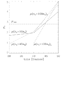
Figure 7: Evolution of the mass-to-flux ratio (MFR, denoted $\mu$ in these plots), normalized to the critical value, in cores formed in numerical simulations of continuously driven MHD isothermal turbulence by Vázquez-Semadeni et al. (2005a). The cores are defined as connected sets of grid cells with density above a density threshold $n_{\rm t}$, and are followed over time. Three values of $n_{\rm t}$ are used, illustrating how the value of the MFR depends and evolves as successively more internal regions of the density fluctuation are considered. Left: Evolution of $\lambda$ in a core that does not collapse. At all values of $n_{\rm t}$, the MFR first increases and then decreases again. Right: A core that does collapse. In this panel, two lines are shown at the largest value of $n_{\rm t}$, because the parent clump splits into two cores at this threshold. In both panels, the rate of variation of $\lambda$ is larger for larger values of $n_{\rm t}$, and $\lambda$ for the innermost region ($n_{\rm t}=100n_{0}$, where $n_{0}$ is the mean density of the simulation) is seen to start lower than that of the envelope, and to overtake it as the degree of mass concentration is increased, in this case as a consequence of numerical diffusion, which plays a role analogous to that of AD.

Note also that, as discussed in §3.3, the mass of the clump must be evolving in time. If the compression is occurring mostly along field lines (since in this direction the magnetic field presents no resistance to it), then the magnetic flux remains roughly constant, while the mass increases at first, and later it possibly decreases if the clump begins to re-expand. Otherwise, if the core becomes massive enough that it becomes gravitationally unstable and supercritical, it must begin to collapse gravitationally (Fig. 7). At this point, the rapid density enhancement at the core in turn enhances the action of AD (e.g., Shu et al., 1987; Mouschovias, 1991, see also §3.1), causing the magnetic flux to escape the core, so that the latter eventually acquires a larger value of $\lambda$ than its envelope. Thus, the prediction from this dynamic scenario of core formation is that cores in early stages of evolution should exhibit smaller values of the MFR than their envelopes, while cores at more advanced stages should exhibit larger values of the MFR than their envelopes. Evidence in this direction has begun to be collected observationally (Crutcher et al., 2009), as well as through synthetic observations of numerical simulations (Lunttila et al., 2009).

Before closing this section, an important remark is in order. Recent numerical and observational evidence (cf. Sec 5.5) suggests that the “turbulence” in star-forming molecular clouds may actually consist of a hierarchy of gravitational contraction motions, rather than of random, isotropic turbulence. In such a case, the physical processes discussed in this section are still applicable, noting that the converging flows that produce the clumps may be driven by larger-scale gravitational collapse rather than by random turbulent compressions, and the only part of the previous discussion that ceases to be applicable is the possibility that some cores may fail to collapse and instead re-expand. If the motions all have a gravitational origin, then essentially all cores must be on their way to collapse. It is worth pointing out that in this case, what drives the collapse of an apparently subcritical core is the collapse of its parent, supercritical structure.

4 Turbulence in the Multiphase ISM

In the previous sections we have separately discussed two different kinds of physical processes operating in the ISM: radiative heating and cooling, and compressible MHD turbulence in the special case of isothermality. However, since both operate simultaneously in the atomic ISM, it is important to understand how they interact with each other, especially because the mean density of the Galactic ISM at the Solar galactocentric radius, $\langle n\rangle\sim 1{\rm~{}cm}^{-3}$, falls precisely in the thermally unstable range. This problem has been investigated numerically by various groups (e.g., Hennebelle & Pérault, 1999, 2000; Walder & Folini, 2000; Koyama & Inutsuka, 2000, 2002; Vázquez-Semadeni et al., 2000a, 2003a, 2006, 2007, 2011; Hennebelle etal., 2008; Banerjee et al., 2009; Gazol et al., 2001, 2005, 2009; Kritsuk & Norman, 2002; Sánchez-Salcedo et al., 2002; Piontek & Ostriker, 2004, 2005; Audit & Hennebelle, 2005, 2010; Heitsch et al., 2005; Hennebelle & Audit, 2007), and in this section we review their main results.

4.1 Density PDF in the Multiphase ISM

A key parameter controlling the interaction between turbulence and net cooling is the ratio $\eta\equiv\tau_{\rm c}/\tau_{\rm t}$, where $\tau_{\rm c}\sim kT/(n\Lambda)$ is the cooling time, with $k$ being the Boltzmann constant, and $\tau_{\rm t}\sim L/U$ is the turbulent crossing time. The remaining symbols have been defined above. In the limit $\eta\gg 1$, the dynamical evolution of the turbulent compreesions occurs much more rapidly than they can cool, and therefore the compressions behave nearly adiabatically. Conversely, in the limit $\eta\ll 1$, the fluctuations cool down essentially instantaneously while the turbulent compression is evolving, and thus they tend to reach the thermal equilibrium pressure $P_{\rm eq}$ as soon as they are produced (Elmegreen, 1991; Passot et al., 1995; Sánchez-Salcedo et al., 2002; Vázquez-Semadeni et al., 2003a; Gazol et al., 2005). Because in a turbulent flow velocity fluctuations of a wide range of amplitudes and size scales are present, the resulting density fluctuations in general span the whole range between those limits, and the actual thermal pressure of a fluid parcel is not uniquely determined by its density, but rather depends on the details of the velocity fluctuation that produced it. This causes a scatter in the values of the pressure around the thermal-equilibrium value in the pressure-density diagram (Fig. 8, left panel), and also produces significant amounts of gas (up to nearly half of the total mass) with densities and temperatures in the classically forbidden thermally unstable range (Gazol et al., 2001; de Avillez & Breitschwerdt, 2005; Audit & Hennebelle, 2005; Mac Low et al., 2005), a result that has been encountered by various observational studies as well (e.g., Dickey et al., 1978; Heiles, 2001). In any case, the tendency of the gas to settle in the stable phases still shows up as a multimodality of the density PDF, which becomes less pronounced as the rms turbulent velocity increases (Fig. 8, right panel).

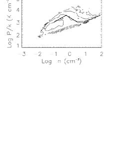
Figure 8: Left: Two-dimensional histogram of the grid cells in the pressure-density diagram for a two-dimensional simulation of turbulence in the thermally-bistable atomic medium, with rms velocity dispersion of $9~{}{\rm km~{}s}^{-1}$, a numerical box size of 100 pc, and the turbulent driving applied at a scale of 50 pc. Right: Density PDF in simulations like the one on the left panel, but with three different values of the rms velocity: $4.5~{}{\rm km~{}s}^{-1}$ (solid line), $9~{}{\rm km~{}s}^{-1}$ (dotted line), and $11.3~{}{\rm km~{}s}^{-1}$ (dashed line). The bimodality of the PDF is seen to to become less pronounced as the rms velocity increases, with a single power-law tail developing in the density range between the values where the peaks would be otherwise located. From Gazol et al. (2005).

4.2 The Formation of Dense, Cold Clouds and Clumps

The Non-Magnetic Case

A very important consequence of the interaction of turbulence (or, more generally, large-scale coherent motions of any kind) and TI is that the former may nonlinearly induce the latter. Indeed, Hennebelle & Pérault (1999, see also Koyama & Inutsuka 2000) showed that transonic (i.e., with $M_{\rm s}\sim 1$) compressions in the WNM can compress the medium and bring it sufficiently far from thermal equilibrium that it can then undergo a phase transition to the CNM (Fig. 9, left panel). This process amounts then to producing a cloud with a density up to $100\times$ larger than that of the WNM by means of only moderate, transonic compressions. This is in stark contrast with the process of producing density fluctuations by pure supersonic compressions in, say, an isothermal medium, in which such density contrasts would require Mach numbers $M_{\rm s}\sim 10$. It is worth noting that the turbulent velocity dispersion of $\sim 8$–11$~{}{\rm km~{}s}^{-1}$ in the warm Galactic ISM (Kulkarni & Heiles, 1987; Heiles & Troland, 2003) is, precisely, transonic.

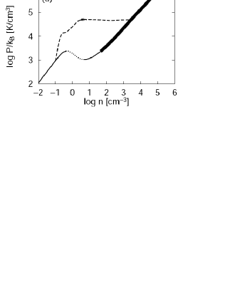
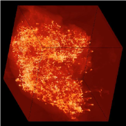
Figure 9: Left: Evolutionary path (dashed line) in the $P$ vs. $\rho$ diagram of a fluid parcel initially in the WNM after suffering a transonic compression that nonlinearly triggers TI. The solid and dotted lines show the locus of $P_{\rm eq}(\rho)$, the solid sections corresponding to linear stability and the dotted ones to linear instability. The solid section to the left of the dotted line corresponds to the WNM and the one at the right, to the CNM. The perturbed parcel evolves from left to right along the dashed line. From Koyama & Inutsuka (2000). Right: Projected (or column) density structure of the resulting GMC in a numerical simulation of its formation by colliding WNM streams, and its subsequent evolution. The numerical box has a size of 15 pc on a side, and the resolution is $1200^{3}$ grid cells. The “GMC” is seen to consist of the agglomeration of a huge number of small clumps, which have formed by fragmentation caused by the action of combined instabilities in the compressed gas. From Audit & Hennebelle (2010).

Moreover, the cold clouds formed by this mechanism have typical sizes given by the size scale of the compressive wave in the transverse direction to the compression, rather than having to be of the same size scale as the fastest growing mode of TI, which is very small ($\lower 2.15277pt\hbox{$\;\buildrel<\over{\sim}\;$}0.1$ pc; cf. §2). The initial stages of this process may produce thin CNM sheets (Vázquez-Semadeni et al., 2006), which are in fact observed (Heiles & Troland, 2003). However, such sheets are quickly destabilized, apparently by a combination of nonlinear thin shell (NTSI; Vishniac, 1994), Kelvin-Helmholtz and Rayleigh-Taylor instabilities (Heitsch et al., 2005), fragmenting and becoming turbulent. This causes the clouds to become a complex mixture of cold and warm gas, where the cold gas is distributed in an intrincate network of sheets, filaments and clumps, possibly permeated by a dilute, warm background. An example of this kind of structure is shown in the right panel of Fig. 9.

A noteworthy feature of the clouds and clumps formed by TI is that, contrary to the case of density fluctuations in single-phase media, they can have more clearly defined and long-lasting boundaries. This is because their boundaries may be defined by the locus of the interface between the cold and warm phases, which, once formed, tends to persist over long timescales compared to the dynamical time, because the two phases are essentially at the same pressure. Under quasi-hydrostatic conditions, these boundaries would have little or no mass flux across them (i.e., they are contact discontinuities; see, e.g., Shu, 1992). Any mass exchange that managed to happen would be due to evaporation or condensation, occurring when the thermal pressure differs from the saturation value between the phases (e.g., Zel’Dovich & Pikel’Ner, 1969; Penston & Brown, 1970; Nagashima et al., 2005; Inoue et al., 2006). The latter two papers have in fact proposed that such evaporation may contribute to the driving of interstellar turbulence, although the characteristic velocities they obtained ($\lower 2.15277pt\hbox{$\;\buildrel<\over{\sim}\;$}1~{}{\rm km~{}s}^{-1}$) appear to be too small for this to be the dominant mechanism for driving the large scale ISM turbulence, with characteristic speeds of $\sim 10~{}{\rm km~{}s}^{-1}$.

However, in the presence of large-scale ($>10$ pc) and large-amplitude ($\lower 2.15277pt\hbox{$\;\buildrel>\over{\sim}\;$}10$ km s^-1) motions, corresponding either to the supernova-driven global ISM turbulence, to larger-scale instabilities, such as the magneto-Jeans (e.g., Kim & Ostriker, 2001) or magneto-rotational (Balbus & Hawley, 1991) ones, or simply to the passage of spiral arms, the nonlinear triggering of TI implies that the fronts bounding the clouds and clumps are not contact discontinuities, but rather phase transition fronts – structures analogous to shocks, with large density, temperature and velocity jumps, but without the need for locally supersonic velocities. Across such fronts, a substantial mass flux occurs (Vázquez-Semadeni et al., 2006; Banerjee et al., 2009). This is mechanism is illustrated in Fig. 10, which clearly shows the rapid growth of a clump by accretion of diffuse material in a numerical simulation. This is in stark contrast with early ideas that the clumps grew by coagulation of tiny cloudlets on very long timescales ($\sim 100$ Myr; e.g., Kwan, 1979).

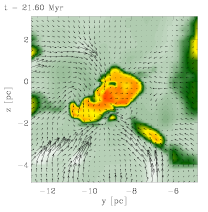
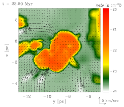
Figure 10: Density cuts through the plane $x=2.5$ pc in an adaptive-mesh refinement (AMR) numerical simulation of molecular cloud formation by Banerjee et al. (2009), illustrating the clump growth mechanism. The numerical box size is 256 pc, and the maximum resolution is 0.06 pc. The arrows show the projection of the velocity field on this plane. Left: The clump at time $t=21.6$ Myr. Right: The clump at $t=22.5$ Myr. Comparing the two times the growth of the clump is evident. The velocity field is seen to generally point towards the clump, indicating that material from the diffuse external medium is entering the clump, causing its growth.

It should be emphasized, however, that the density does not necessarily always present a sharp jump between the clump and its surroundings. As discussed in §4.1, the presence of turbulence in the diffuse medium also implies a certain degree of mixing, and the existence of a certain fraction of the mass that is traversing the unstable range. In Fig. 10 this can be observed as the greenish regions, especially near the right edge of the left panel.

We conclude then that, although in thermally bistable flows clump boundaries are in general better defined than in turbulent isothermal flows because of the density jumps induced by the thermal bistability, this does not imply that they are impenetrable boundaries that restrict the flow of the medium. Rather, the clumps are formed and then grow by accretion of diffuse material across these phase transition fronts.

Finally, it is important to note that, in the scenario of GMC formation described above, the compressions in the WNM tend to initially form thin sheets of CNM (Vázquez-Semadeni et al., 2006), in agreement with observations of CNM clouds (Heiles & Troland, 2003). These sheets, however, grow by accretion of diffuse gas, fragmenting and becoming turbulent due to the combined action of various instabilities (Vázquez-Semadeni et al., 2006; Heitsch et al., 2006), so that GMCs may actually consist of huge conglomerates of small clumps, as illustrated in the right panel of Fig. 9. This is consistent with the observed clumpy structure of GMCs (Blitz, 1993, sec. VII).

The Magnetic Case

In the presence of a magnetic field, the process of cloud formation by phase transitions to the cold phase requires further considerations. First, the orientation of the compressive motion relative to that of the magnetic field strongly influences the ability of the compression to trigger a transition to the dense phase. Hennebelle & Pérault (2000) investigated this problem by means of numerical simulations with slab (1+1/2D) geometry, finding that, for a certain value of the magnetic field strength, and a given sonic Mach number of the compression, there exists a maximal angle between the direction of compression and the direction of the magnetic field beyond which no phase transition is induced. They found this angle to typically lie between 20 to 40 degrees, for typical values of the warm neutral medium.

Hennebelle & Pérault (2000) also found that, when the formation of a cloud does occur, either the field is re-oriented along the compression (in the case of weak fields), or the flow is re-oriented along field lines (in the case of strongter fields), and the accumulation of gas to form the clump ends up being aligned with the magnetic field. In addition, Inoue & Inutsuka (2008) have found that compressions perpendicular to the magnetic field strongly inhibit the formation of dense, molecular-type clouds, and that, in this case, only diffuse HI clouds manage to form. As a consequence, the discussion of cloud formation can be made in terms of compressions parallel to the magnetic field without loss of generality. We will take up this problem again in §5.5, when we discuss the onset of gravitational collapse of the clouds.

5 The Nature of the Turbulence in the various ISM Components

5.1 Generalities

As discussed in the previous sections, the ionized and atomic components of the ISM consist of gas in a wide range of temperatures, from $T\sim 10^{6}$ K for the HIM, to $T\sim 40$ K for the CNM. In particular, Heiles & Troland (2003) report temperatures in the range $500<T<10^{4}$ K for the WNM, and in the range $10<T<200$ K for the CNM. The WIM is expected to have $T\sim 10^{4}$ K. This implies that the adiabatic sound speed, given by (e.g., Landau & Lifshitz, 1959)

$$c_{\rm s}=\sqrt{\frac{\gamma kT}{\mu_{\rm m}m_{\rm H}}}\approx 10.4~{}{\rm km~{}s}^{-1}\left(\frac{T}{10^{4}{\rm K}}\right)^{1/2},$$ (17)

will also exhibit large fluctuations in the medium. In the second equality, we have used $\mu_{\rm m}=1.27$. In the following sections we discuss the implications of these ranges for the various ISM components.

5.2 The Hot Ionized medium

At temperatures $T\sim 10^{6}$ K, the sound speed in the HIM is $\sim 100~{}{\rm km~{}s}^{-1}$, much larger than the velocity dispersion in the general ISM, $\sim 10~{}{\rm km~{}s}^{-1}$. Thus, except in the immediate vicinity of supernova explosions, where the velocities can reach thousands of$~{}{\rm km~{}s}^{-1}$, the HIM in general is expected to behave nearly incompressibly. Moreover, because the density is very low ($\lower 2.15277pt\hbox{$\;\buildrel<\over{\sim}\;$}10^{-2}{\rm~{}cm}^{-3}$), the cooling time ($\tau_{\rm c}\sim kT/n\Lambda$; cf. Sec. 4.1) is very long (a few tens of Myr), and the medium is then expected to behave roughly adiabatically, at least up to scales of a few hundred parsecs.

5.3 The Warm Ionized Medium

Collecting measurements of interstellar scintillation (fluctuations in amplitude and phase of radio waves caused by scattering in the ionized ISM) from a variety of observations, Armstrong et al. (1995) estimated the power spectrum of density fluctuations in the WIM, finding that it is consistent with a Kolmogorov (1941) spectrum, a result expected for weakly compressible flows (Bayly et al., 1992), on scales $10^{8}\lower 2.15277pt\hbox{$\;\buildrel<\over{\sim}\;$}L\lower 2.15277pt\hbox{$\;\buildrel<\over{\sim}\;$}10^{15}$ cm.

More recently, using data from the Wisconsin H$\alpha$ Mapper Observatory, Chepurnov & Lazarian (2010) have been able to extend the spectrum to scales $\sim 10^{19}$ cm, suggesting that the WIM behaves as an incompressible turbulent flow over size scales spanning more than 10 orders of magnitude. This suggestion is supported also by the results of Hill et al. (2008) who, by measuring the distribution of H$\alpha$ emission measures in the WIM, and comparing with numerical simulations of turbulence at various Mach numbers, concluded that the sonic Mach number of the WIM should be $\sim 1.4$–2.4. Although the WIM is ionized, and thus should be strongly coupled to the magnetic field, the turbulence then being magnetohydrodynamic (MHD), Kolmogorov scaling should still apply, according to the theory of incompressible MHD fluctuations (Goldreich & Sridhar, 1995). The likely sources of kinetic energy for these turbulent motions are stellar energy sources such as supernova explosions (see, e.g., Mac Low & Klessen, 2004).

5.4 The Atomic Medium

In contrast to the relatively simple and clear-cut situation for the ionized ISM, the turbulence in the neutral (atomic and molecular) gas is more complicated. According to the discussion in §5.1, the temperatures in the atomic gas may span a continuous range from a few tens to several thousand degrees. Additionally, Heiles & Troland (2003) report column density-weighted rms velocity dispersions $\sigma_{v}\sim 11~{}{\rm km~{}s}^{-1}$ for the WNM, and typical internal motions of $M_{\rm s}\sim 3$ for the CNM. It is thus clear that the WNM is transonic ($M_{\rm s}\sim 1$), while the CNM is moderately supersonic. This occurs because the atomic gas is thermally bistable, and because transonic compressions in the WNM can nonlinearly induce TI and thus a phase transition to the CNM (§4.1). Thus, the neutral atomic medium is expected to consist of a complex mixture of gas spanning over two orders of magnitude in density and temperature.

It is worth noting that early pressure-equilibrium models (e.g., Field et al., 1969; McKee & Ostriker, 1977) proposed that the unstable phases were virtually nonexistent in the ISM, but the observational and numerical results discussed in §4.1 suggest that a significant fraction of the atomic gas mass lies in the unstable range, transiting between the stable phases. Also, numerical simulations of such systems suggest that the velocity dispersion within the dense clumps is subsonic, but that the velocity dispersion of the clumps within the diffuse substrate is supersonic with respect to their internal sound speed (although subsonic with respect to the warm gas; Koyama & Inutsuka, 2002; Heitsch et al., 2005).

5.5 The Molecular Gas

Molecular Clouds: Supersonically Turbulent, or Collapsing?

The evidence

Molecular clouds (MCs) have long been known to be strongly self-gravitating (e.g., Goldreich & Kwan, 1974; Larson, 1981). In view of this, Goldreich & Kwan (1974) initially proposed that MCs should be in a state of gravitational collapse, and that the observed motions in MCs (as derived by the non-thermal linewidths of molecular lines) corresponded to this collapse. However, shortly thereafter, Zuckerman & Palmer (1974) argued against this possibility by noting that, if all the molecular gas in the Galaxy, with mean density $n\sim 100{\rm~{}cm}^{-3}$ and total mass $M_{\rm mol}\sim 10^{9}M_{\odot}$, were in free-fall, then a simple estimate of the total SF rate (SFR) in the Galaxy, given by SFR $\sim M_{\rm mol}/\tau_{\rm ff}\sim 200~{}M_{\odot}$ yr^-1, where $\tau_{\rm ff}=\sqrt{3\pi/32G\rho}$ is the free-fall time, would exceed the observed rate of $\sim 2~{}M_{\odot}$ yr^-1 (e.g., Chomiuk & Povich, 2011) by about two orders of magnitude. Moreover, Zuckerman & Evans (1974) argued that, if clouds were undergoing large-scale radial motions (a regime which they assumed would include the case of a global gravitational contraction), then the star formation activity, and the Hii regions associated with it, would tend to be concentrated at the center of the cloud. Under these conditions, the H₂CO absorption lines seen on the spectra of the Hii regions, produced by the surrounding, infalling gas, should be redshifted with respect to the CO lines produced by the cloud as a whole, an effect which Zuckerman & Evans (1974) showed does not occur. They also argued that such a “radial-motion” flow regime is inconsistent with the fact that clouds contain multiple Hii regions, clusters, and dense clumps. A related notion, which still persists today, is that, if a cloud is undergoing global collapse, the largest linewidths should occur near the collapse center, as the infall velocities should be at a maximum there, contrary to the observation that the largest velocity dispersions occur at the largest scales (Larson, 1981).

These objections prompted the suggestion (Zuckerman & Evans, 1974) that the non-thermal motions in MCs corresponded instead to small-scale (in comparison to the sizes of the clouds) random turbulent motions. The need for these motions to be confined to small scales arose from the need to solve the absence of a systematic shift between the H₂CO absorption lines of Hii regions and the CO lines from their parent molecular clouds noted by those authors. But such a small-scale nature also had the advantage that the turbulent (ram) pressure could provide an approximately isotropic pressure that could counteract the self-gravity of the clouds at large, thus providing a suitable mechanism for keeping the clouds from collapsing and maintaining them in near virial equilibrium (Larson, 1981). On the other hand, because turbulence is known to be a dissipative phenomenon (e.g., Landau & Lifshitz, 1959), research then focused on finding suitable sources for driving the turbulence and avoiding rapid dissipation. The main driving source was considered to be energy injection from stars (e.g., Norman & Silk, 1980; McKee, 1989; Li & Nakamura, 2006; Nakamura & Li, 2007; Krumholz et al., 2006; Carroll et al., 2009, 2010; Wang et al., 2010, see also the reviews by Mac Low & Klessen 2004 and Vázquez-Semadeni 2010), and reduction of dissipation was proposed to be accomplished by having the turbulence being MHD, and consisting mostly of Alfvén waves, which were thought not to dissipate as rapidly (e.g., Shu et al., 1987), and which could provide an isotropic pressure (McKee & Zweibel, 1995).

However, in the last decade several results have challenged the turbulent pressure-support scenario: 1) Turbulence is known to be characterized by having the largest velocity differences occurring at the largest scales, and MCs are no exception, exhibiting scaling relations between velocity dispersion and size which suggest that the largest velocity differences occur at the largest scales (Larson, 1981; Heyer & Brunt, 2004; Brunt et al., 2009, Fig. 11, left and middle panels). This is inconsistent with the small-scale requirement for turbulent support. 2) It was shown by several groups that MHD turbulence dissipates just as rapidly as hydrodynamic turbulence (Mac Low et al., 1998; Stone et al., 1998; Padoan & Nordlund, 1999), dismissing the notion of reduced dissipation in “Alfvén-wave turbulence”, and thus making the presence of strong driving sources for the turbulence an absolute necessity. 3) Clouds with very different contributions from various turbulence-driving mechanisms, including those with little or no SF activity, such as the so-called Maddalena’s cloud (Maddalena & Thaddeus, 1985), show similar turbulence characteristics (Williams et al., 1994; Schneider et al., 2011), suggesting that stellar energy injection may not be the main source of turbulence in MCs.

Figure 11: Left and middle panels: Second eigenimages obtained by Principal Component Analysis of spectroscopic data of the star-forming region NGC 1333, showing the main contribution to the linewidth of molecular emission in this region (Brunt et al., 2009). The middle image shows the region enclosed in the rectangle in the left image. Black and white colors represent oppositely-signed components of the velocity. Brunt et al. (2009) describe the pattern as a “dipole”, in which large-scale patches of alternating velocity direction are observed. This is seen in both the large-scale (left) and the small-scale (middle) images. Right panel: Image of the projected density field of a 3D numerical simulation with cooling, self-gravity, and magnetic fields, representing the formation of a dense atomic cloud by the collision of WNM streams in the direction perpendicular to the plane of the figure. The time shown is 20 Myr after the start of the simulation. The black dots denote “sink” particles, which replace local collapsing zones in the simulation. The whole cloud is also collapsing, although its collapse is not completed yet by the end of the simulation, at $t=31$ Myr. From Vázquez-Semadeni et al. (2011).

Moreover, simulations of dense cloud formation in the nonmagnetic case have shown that, once a large cold CNM cloud forms out of a collision of WNM streams, it quickly acquires a large enough mass that it can begin to collapse gravitationally in spite of it being turbulent (Vázquez-Semadeni et al., 2007, 2010; Heitsch & Hartmann, 2008; Heitsch et al., 2008a). This happens because, as the atomic gas transitions from the warm to the cold phase, its density increases by roughly two orders of magnitude, while the temperature drops by the same factor. Thus, the Jeans mass in the gas, proportional to the product $n^{-1/2}T^{3/2}$, drops by a factor $\sim 10^{4}$, implying that the cold cloud assembled by the compression can rapidly exceed its Jeans mass.

In turn, the gravitational contraction very effectively enhances the column density of the gas, promoting the formation of molecular hydrogen (H₂) (Hartmann et al., 2001; Bergin et al., 2004; Heitsch & Hartmann, 2008), and so it appears that the formation of a molecular cloud may involve some previous gravitational contraction (see also McKee, 1989). In addition, according to the discussion in Secs. 4.2 and 5.4, the CNM clouds formed by converging WNM flows should be born turbulent and clumpy. This turbulent nature of the clouds further promotes the formation of molecular hydrogen (Glover & Mac Low, 2007). The simulations (Vázquez-Semadeni et al., 2007, 2010; Heitsch & Hartmann, 2008) show that the nonlinear, turbulent density fluctuations can locally complete their collapse before the global collapse of the cloud is completed (Fig. 11, right panel), both because their densities are large enough that their free-fall time is significantly shorter than that of the whole cloud (Heitsch & Hartmann, 2008; Pon et al., 2011), and because clouds in general have flattened or filamentary shapes (e.g., Bally et al., 1989; de Geus et al., 1990; Heiles & Troland, 2003; Molinari et al., 2010; André et al., 2010). Interestingly, the free-fall time for these geometries may be much larger than the standard free-fall time, $\tau_{\rm ff}=\sqrt{3\pi/32G\rho}$, which is applicable to a spherically symmetric structure (Toalá et al., 2012; Pon et al., 2012). Thus, an approximately spherical clump of the same volume density within a flattened or elongated structure can collapse much earlier than the non-spherical cloud in which it is immersed.

In addition, the turbulent velocities initially induced in the clouds by the converging flows in the simulations are observed to be relatively small (only moderately supersonic [$M_{\rm s}\sim 3$] with respect to the dense gas). Strongly supersonic ($M_{\rm s}\sim 10$) velocities like those observed in real molecular clouds only develop later in the simulations, due to the ensuing gravitational contraction (Vázquez-Semadeni et al., 2007). This is in agreement with the fact that CNM clouds are observed to typically have moderately supersonic ($M_{\rm s}\sim 3$) velocity dispersions (Heiles & Troland, 2003), while GMCs are observed to have much larger turbulent rms Mach numbers, $M_{\rm s}\sim 10$–20 (Wilson et al., 1970). Finally, Banerjee et al. (2009) noted that, in their numerical simulations, the clumps with highest internal velocity dispersions were those that had already formed collapsed objects (“sink” particles), even though energy feedback from the sinks was not included. This again suggested that the largest velocities develop by the action of self-gravity.

Do observations rule out global gravitational contraction in star-forming molecular clouds?

It is very important to note that the possibility of MCs being in gravitational collapse is not in contradiction with any observed properties of MCs. First, as noted by Ballesteros-Paredes et al. (2011a), the magnitudes of the virial and free-fall velocities for a self-gravitating object are observationally indistinguishable. Thus, the interpretation of cloud energetics in terms of virial equilibrium is completely interchangeable by an interpretation of collapse.

Also, one important argument against the possibility of gravitational collapse of MCs is the argument by Zuckerman & Palmer (1974) that it would lead to exceedingly large SFRs. We discuss the possible resolution of this conundrum in §6.2. Another frequent argument against the global gravitational contraction scenario is that such a regime should produce readily observable signatures, such as the systematic shift between the CO lines from the clouds and the absorption lines seen towards Hii regions proposed by Zuckerman & Evans (1974), as discussed at the beginning of this section. However, it should be noted that the argument by ZE74 against large-scale motions in the clouds would also apply to turbulent motions as we presently understand them, since turbulent flows in general have the largest velocity differences across the largest velocity separations, as discussed above in relation to the left and middle panels of Fig. 11. The only kind of turbulence that would not be invalidated by ZE74’s argument would be microscopic turbulence, in which the largest turbulent scale should be much smaller than the size of the cloud, but, as already discussed above, this is clearly not the case in molecular clouds, as illustrated by the left and middle panels of Fig. 11.

Moreover, the above arguments against global collapse in clouds are based on the assumptions that the cloud has a roughly spherical symmetry, and that the collapse is monolithic, meaning that there is a single, dominant flow, aimed at a major, localized collapse center. Actually, numerical simulations of cloud formation and evolution show that this is not the case. As mentioned above, the clouds are far from having a spherical symmetry, and instead tend to have flattened or filamentary shapes. In addition, the clouds are born turbulent, and therefore they contain nonlinear density fluctuations, which have shorter free-fall times than the average in the cloud, and thus collapse earlier. Thus, multiple collapse centers arise in the cloud before the global collapse is completed, and, as a consequence, there is no single, evident, dominant collapse center, possibly resolving the concerns of Zuckerman & Evans (1974). Essentially, the cloud fragments gravitationally, with the local collapse centers accreting from filaments that in turn accrete from the bulk of the cloud (Gómez & Vázquez-Semadeni, in prep.), in agreement with the structure of clumps and their surrounding filaments (Myers, 2009; André et al., 2010; Palmeirim et al., 2013). Towards the end of the evolution, the locally collapsing regions formed earlier tend to merge to form a massive region then acquires large densities and velocities, typical of massive-star forming regions (Vázquez-Semadeni et al., 2009). This flow regime has been termed hierarchical, chaotic gravitational fragmentation (Vázquez-Semadeni et al., 2009; Ballesteros-Paredes et al., 2011a).

Note, however, that all of the above arguments in favor of gravitational contraction motions in MCs probably apply mostly to clouds in the early-to-intermediate stages of their evolution; that is, from their formation to their strongly star-forming stages. Nevertheless, after strong stellar feedback has disrupted the clouds, it is likely that shreds may remain that may remain in a relatively quiescent stage, perhaps supported by the magnetic field, without forming stars, and perhaps even being on their way to dispersal (Elmegreen, 2007; Vázquez-Semadeni et al., 2011).

All of the above evidence suggests that the observed supersonic nonthermal motions in MCs may evolve from being dominated by random turbulence in the early evolutionary stages of the (mostly atomic) clouds, to being infall-dominated at more advanced (mostly molecular) stages, characterized by large densities, velocities, and star formation rates. Note, however, that the turbulent component may be maintained or even somewhat amplified by the collapse (Vázquez-Semadeni et al., 1998; Robertson & Goldreich, 2012).

In this scenario of hierarchical gravitational fragmentation, the main role of the truly turbulent (i.e., fully random) motions is to provide the nonlinear density fluctuation seeds that will collapse locally once the global contraction has caused their density to increase sufficiently for them to become locally gravitationally unstable (Clark & Bonnell, 2005). Evidence for such multi-scale collapse has recently begun to be observationally detected (Galván-Madrid et al., 2009; Schneider et al., 2010).

The Molecular Gas. Results Including the Magnetic Field

According to the discussion in §4.2, the formation of a cold, dense atomic cloud can be accomplished by the compression of warm material along magnetic field lines, which nonlinearly triggers a phase transition to the cold phase. However, as discussed in the previous section, the formation of a molecular cloud probably requires the gravitational contraction of the atomic cloud previously formed by the compression. Thus, in the presence of the magnetic field, this requires an understanding of the role of magnetic support; that is, of the evolution of the mass-to-flux ratio (MFR).

As is well known, and was reviewed in §3.4, there exists a critical value of the MFR below which the magnetic field is able to support the cloud against its own self-gravity. Along the direction of the field lines, the criticality condition in terms of the mass column density $\Sigma=\rho L$ and the field strength $B_{0}$ for a cylindrical geometry is (Nakano & Nakamura, 1978),

$$\left(\Sigma/B_{0}\right)_{\rm crit}=(4\pi^{2}G)^{-1/2}\approx 0.16~{}G^{-1/2},$$ (18)

where $\rho$ is the mass density and $L$ is the cylinder length. This condition gives the accumulation length, in terms of fiducial values representative of the ISM in the solar neighborhood, as (Hartmann et al., 2001)

$$L_{\rm c}\approx 470\left(\frac{B_{0}}{5\lambda{\rm G}}\right)\left(\frac{n}{1{\rm~{}cm}^{-3}}\right)^{-1}~{}{\rm pc},$$ (19)

where we have assumed $\mu_{\rm m}=1.27$. In principle, if the Galactic field is primarily azimuthal, then the Galactic ISM at large is magnetically supercritical in general, because field lines circle around the entire Galactic disk, and thus sufficiently long distances are always available along them. Thus, the MFR of a system is not a uniquely defined, absolute parameter, but rather depends on where the boundaries of the system are drawn. Also, recall that the critical value of the MFR depends on the local geometry of the system being considered. For instance, a system with spherical symmetry has a critical value of $(\Sigma/B_{0})_{\rm crit}=(6\pi^{2}G)^{-1/2}\approx 0.13~{}G^{-1/2}$ (e.g. Shu, 1992), somewhat smaller than that given by eq. (18).

Now consider a cloud or clump that is formed by the accumulation of gas along field lines in general. In the rest of this discussion, we will generically refer to the resulting density enhancement as a “cloud”, referring to either a cloud, a clump, or a core. Although redistribution of matter along field lines does not in principle affect the total MFR along the full “length” of a flux tube, this length is a rather meaningless notion, since the flux tube may extend out to arbitrarily long distances. What is more meaningful is the MFR of the dense gas that makes up the cloud, since the cloud is denser than its surroundings, and thus it is the main source of the self-gravity that the field has to oppose. In fact, for the formation of a cloud out of flow collisions in the WNM, the density of the cloud is $\sim 100$ times larger than that of the WNM (Field et al., 1969; Wolfire et al., 1995), and so the self-gravity of the latter is negligible. Thus, in this problem, natural boundaries for the cloud are provided by the locus of the phase transition front between the dense and the diffuse gas, allowing a clear working definition of the MFR.

However, contrary to the very common assumption of a constant cloud mass, the formation of clouds by converging gas streams implies that the mass of the cloud is a (generally increasing) function of time (cf. §3.3), a conclusion that has recently been reached observationally as well (Fukui et al., 2009). This means that, within the volume of the cloud, the MFR is also an increasing quantity, since the flux remains constant if the flow is along field lines, while the mass increases (see also Shu et al., 2007). If the cloud starts from essentially zero mass, this in turn implies that the MFR of a cloud is expected to start out strongly subcritical (when the cloud is only beginning to appear), and to evolve towards larger values at later times. Rewriting eq. (19) for the column density, we see that the cloud becomes supercritical when (Vázquez-Semadeni et al., 2011)

$$N_{\rm cr}\approx 1.5\times 10^{21}\left(\frac{B_{0}}{5\mu{\rm G}}\right){\rm~{}cm}^{-2},$$ (20)

where $N\equiv\Sigma/\mu_{\rm m}m_{H}$ is the number column density, and is to be measured along the field lines. The critical column density for magnetic criticality given by eq. (20) turns out to be very similar, at least for solar neighbourhood conditions, to the critical column density of hydrogen atoms necessary for cold atomic gas to become molecular, $N_{\rm H}\sim 1$–2$\times 10^{21}{\rm~{}cm}^{-2}$ (e.g., Franco & Cox, 1986; van Dishoeck & Black, 1988; van Dishoeck & Blake, 1998; Hartmann et al., 2001; Glover & Mac Low, 2007, 2007b; Glover et al., 2010).

Moreover, the critical column density given by eq. (20) is also very similar to that required for rendering cold gas gravitationally unstable, which is estimated to be

$$N_{\rm grav}\approx 0.7\times 10^{21}\left(\frac{P/k}{3000~{}K{\rm~{}cm}^{-3}}\right)^{1/2}{\rm~{}cm}^{-2}$$ (21)

(Franco & Cox, 1986; Hartmann et al., 2001). Thus, the evolution of a cloud is such that it starts out as an atomic, unbound, and subcritical diffuse cloud (Vázquez-Semadeni et al., 2006) and, as it continues to accrete mass from the warm atomic medium, it later becomes molecular, supercritical, and collapsing, at roughly the same time (Hartmann et al., 2001). This is fully consistent with the observation that diffuse atomic clouds are in general strongly subcritical (Heiles & Troland, 2005) and not strongly self-gravitating, while GMCs are approximately critical or moderately supercritical (Crutcher, 1999; Bourke et al., 2001; Troland & Crutcher, 2008), and are generally gravitationally bound (e.g., Blitz, 1993).

It is important to note that this is in stark contrast to the SMSF (see, e.g., the reviews by Shu et al., 1987; Mouschovias, 1991), where it was considered that the magnetic criticality of a cloud was the main parameter determining whether it would form only low-mass stars and at a slow pace (in the case of subcritical clouds), or form clusters, including high-mass stars, and at a fast pace (supercritical clouds). This constituted a bimodal scenario of SF, and sub- and supercritical clouds constituted two separate classes.

Instead, in the evolutionary scenario for MCs described above, clouds are expected to evolve from being simultaneously atomic, subcritical and not strongly self-gravitating to being molecular, supercritical and strongly self-gravitating. Next, the roughly simultaneous transition to self-gravitating and supercritical suggests that, in general, GMCs should be in a state of gravitational contraction, at least initially, even in the presence of typical magnetic field strengths in the Galactic disk. Of course, significant scatter in the MFR is expected, both intrinsically (see §3.4) and as a consequence of observational uncertainties (e.g., Crutcher, 1999), and thus a certain fraction of the GMCs may remain subcritical up to significantly evolved stages, or even throughout their entire evolution. This case is discussed further below.

The formation and evolution of molecular clouds in the magnetic case has been investigated recently using numerical simulations of GMC formation by compressions in the WNM aligned with the magnetic field (Hennebelle etal., 2008; Banerjee et al., 2009; Vázquez-Semadeni et al., 2011). The latter authors in particular included self-gravity and AD, and considered three cases: one supercritical, with $\lambda=1.3$, and two subcritical, with $\lambda=0.9$ and 0,7, corresponding to mean field strengths of 2, 3, and 4 $\mu$G, respectively. The initial magnetic field was considered uniform. In all cases, the mean density was $1{\rm~{}cm}^{-3}$ and the temperature $T=5000$ K. The compressions consisted of two oppositely-directed streams of gas at the mean density, and of length 112 pc, immersed in a 256-pc box.

The evolution of the subcritical cases is worth discussing in detail, as it differs somewhat from simple expectations. These simulations produced a dense cloud that quickly began to contract gravitationally, similarly to non-magnetic simulations. This occurred because a uniform magnetic field does not provide any support, since the latter requires the existence of a magnetic gradient. Support builds up gradually as the field lines are bent. The clouds thus contracted for a few tens of Myr, until the magnetic tension was large enough to halt the collapse, at which point they re-expanded, and entered an oscillatory regime, around the equilibrium configuration. However, due to the existence of diffusion (both numerical and from AD), local collapse events managed to occur, in agreement with the notions from the SMSF (see also McKee, 1989). The notable difference with that model, though, occurred in the fact that the clouds only formed stars during the global contraction phase, especially at maximum compression, and essentially shut off in the re-expanding phase. This is in contrast to the SMSF, in which the GMCs at large were assumed to be in equilibrium and forming stars continuously, albeit slowly.

The above discussion suggests that the possibility of star-forming molecular clouds being in a state of gravitational contraction may hold even if they have subcritical MFRs. The subsequent re-expansion of these clouds (or their remnants) may lead to a star-formation-inactive and quiescent phase, perhaps on their way to dispersal, if the clouds are exiting the spiral arms by that time, as proposed by Elmegreen (2007).

6 Star Formation in the Turbulent ISM

6.1 Does Molecular Cloud “Turbulence” Provide Support for Molecular Clouds?

In the previous sections we have discussed how large-scale compressions in the general ISM produce density fluctuations, in particular by nonlinearly inducing phase transitions from the cold to the warm medium. Because the largest dimensions of the clouds thus formed are as large as the transverse dimension of the compression that formed them, and because of the large drop in the local Jeans mass upon the phase transition (cf. Sec. 5.5), they can soon find themselves being strongly gravitationally unstable and proceed to collapse. It is important to note that the large-scale compression forming the clouds may (and in fact, is likely to) have an origin different from the general turbulence in the ISM, such as, for example, large-scale instabilities like the magneto-Jeans one (e.g. Kim & Ostriker, 2001), or simply the passage of the stellar spiral-arm potential well.

In fact, it is worth noting that just the turbulence driven by supernovae does not seem to be able to sustain itself, since the mass driven into a Jeans-unstable regime per unit time by the turbulence is not enough to maintain the same supernova rate that drives the turbulence (Joung & Mac Low, 2006). This conclusion is also supported by the fact that successive generations of triggered SF do not appear to be able to form stars as massive as in the previous generation (Deharveng & Zavagno, 2011). Thus, it appears safe to conclude that the main driver of star formation is gravity at the largest scales.

During the last decade, the main role of interstellar turbulence has been thought to be the regulation of SF, mainly on the basis of the assumption that the turbulent velocity dispersion contributes to the support of molecular clouds against their self-gravity, analogously to the role of the thermal velocity dispersion, and perhaps including a scale-dependent amplitude (Chandrasekhar, 1951; Bonazzola et al., 1987; Bertoldi & McKee, 1992; Vazquez-Semadeni & Gazol, 1995; Mac Low & Klessen, 2004; Krumholz & McKee, 2005; Hennebelle & Chabrier, 2008, 2011; Padoan & Nordlund, 2011). Thus, turbulence has been thought to provide support to clouds as a whole, while simultaneously inducing small-scale density fluctuations (clumps) within the clouds that may undergo gravitational collapse if they are compressed enough for their Jeans mass to become smaller than their actual mass (Vázquez-Semadeni et al., 2003b; Ballesteros-Paredes et al., 2007). In this manner, global collapse of the clouds could be prevented, avoiding the Zuckerman & Palmer (1974) conundrum that the global collapse of molecular clouds would cause an excessively large SFR (see §5.5), while at the same time allowing for the collapse of a small fraction of the mass, brought to instability by the local supersonic turbulent compressions. However, this last notion was challenged by Clark & Bonnell (2005), who argued that the turbulence only provides the seed density fluctuations for subsequent gravitational fragmentation, without significant local reductions in the Jeans mass induced by the turbulence.

Moreover, Heitsch & Hartmann (2008) showed that the fraction of mass with short free-fall times ($\lower 2.15277pt\hbox{$\;\buildrel<\over{\sim}\;$}1$ Myr) in the clouds increases monotonically over time in the presence of self-gravity, indicating a secular evolution towards higher densities, while simulations with no self-gravity exhibited a stationary fraction of mass with short free-fall times, as would be the case in clouds supported against collapse by the turbulence (Fig. 12).

Figure 12: Time evolution of the mass (indicated by the color scale) at a given free-fall time (vertical axis) in numerical simulations of cloud formation and evolution by Heitsch & Hartmann (2008). The top row shows the free-fall time in a linear scale, while the bottom row shows it in logarithmic scale. The panels on the left show a simulation with no self-gravity, while the middle and right panels show two different simulations with self-gravity. In the case with no self-gravity, the fraction of mass at a given free-fall time is seen to remain nearly constant, and the minimum free-fall time to remain at $\sim 1$ Myr, while in the cases with self-gravity, the minimum free-fall time decreases secularly. Note that, in these plots, $\tau_{\rm ff}$ is simply a proxy for the density, since $\tau_{\rm ff}\propto\rho^{-1/2}$, and so it can be evaluated even if gravity is not included in the simulations.

Finally, the simulations have also shown that the fraction of molecular gas also increases in time, so that the cloud would indeed be classified as atomic in its early phases, and as molecular in later ones (Heitsch & Hartmann, 2008; Clark et al., 2012). In particular, the latter authors have shown that the formation of CO-dominated regions only occurs $\sim 2$ Myr before SF starts, although significant amounts of H₂ can appear earlier.

All of the above evidence suggests that the strongly supersonic motions observed in MCs may be a manifestation of the gravitational contraction occurring in the clouds, rather than truly turbulent (i.e., random) motions, of a separate origin, that can counteract the gravitational contraction of the clouds. It is worth noting here that Klessen & Hennebelle (2010) have recently shown that, in general, the accretion power at scales from entire Galactic disks to protostellar disks, passing through the GMC scale, is more than enough to drive the turbulence observed in these systems. However, it should be noted that, in the case of GMCs, this suggestion differs qualitatively from the nature of the motions discussed above. Rather than accretion driving turbulent motions in the clouds which can then support them, the discussion above suggests that the observed motions in the clouds are the infall itself, with only a small, subdominant, truly random turbulent component superposed on them. In this case, these motions cannot provide support against the self-gravity of the clouds.

6.2 Regulation of Star Formation Via Stellar Feedback

All of the above evidence strongly suggests that interstellar clouds undergo a secular evolution, starting their existence as moderatly supersonic, magnetically subcritical, sheet-like atomic clouds, and evolving towards becoming supercritical, molecular, gravitationally contracting objects. However, in this case, the Zuckerman & Palmer (1974) SF conundrum (cf. §5.5) must be addressed. That is, if MCs are essentially in free-fall, how to prevent the SFR from being two orders of magnitude larger than it is observed to be in the Galaxy?

Early studies proposed that ionizing radiation from massive stars should be able to disperse a cloud as early as when only $\sim 10$% of the cloud’s mass has been converted to stars (see, e.g., Sec. 4 of Field, 1970), so that the remaining 90% would be prevented from forming any more stars. This suggestion, however, was challenged by Mouschovias (1976), who argued that those estimates were based on the assumption of unrealistically low mean densities for the clouds ($\sim 10{\rm~{}cm}^{-3}$), and that using more realistic values ($\sim 10^{5}{\rm~{}cm}^{-3}$) would result in a grossly insufficient amount of ionization in the cloud, thus invalidating the mechanism as a suitable one for dispersing the clouds. As an alternative, Mouschovias (1976) proposed the basic notions for the SMSF: that the MCs should be magnetically subcritical in general, so that their envelopes would remain supported by the magnetic tension, while only the central core would be able to proceed to collapse through AD (cf. §§3.1 and 3.4). However, observational evidence from the last decade has suggested that most MCs are likely to be at least moderately magnetically supercritical (e.g., Bourke et al., 2001; Troland & Crutcher, 2008; Crutcher et al., 2010), a conclusion also reached by theoretical arguments (see §5.5 and references therein).

Another alternative was the proposal that MCs could be supported by turbulence, either hydrodynamical or MHD. However, since turbulence needs to be continuously driven, two variants have been considered for the driving: either it might be due to feedback from stellar sources internal to the clouds (cf. §5.5), or else to external driving sources such as supernova shocks. However, as discussed in §§4.2 and 5.5, the role of external turbulence seems more likely to be the driving of MC formation, rather than the driving of the strongly supersonic internal turbulence of the GMCs, because the turbulence induced in the forming clouds is only moderately supersonic, rather than strongly so (cf. §6.1).

The possibility of driving the turbulence by stellar feedback from inside the clouds has been extensively studied, both analytically and numerically (e.g., Norman & Silk, 1980; McKee, 1989; Li & Nakamura, 2006; Nakamura & Li, 2007; Carroll et al., 2009, 2010; Wang et al., 2010). In most such studies, it has been concluded that this feedback can maintain the clumps within GMCs in near virial equilibrum. Studies of the SFR and the SFE under these conditions have often idealized the turbulence as being simply randomly driven, and have shown that in this case the SFE can be maintained at levels of a few percent, comparable to the observed ones (e.g., Klessen et al., 2000; Vázquez-Semadeni et al., 2003a, 2005b).

However, as discussed in the review by Vázquez-Semadeni (2010), numerical simulations of the momentum feedback from protostellar outflows have only considered numerical boxes at the parsec (clump) scale, neglecting the infall from the environment of the clump, which has been observed in GMC formation simulations. This adds a large amount of ram pressure to the system not included in those simulations. Thus, it seems that outflows cannot provide sufficient feedback to prevent the collapse of entire GMCs.

The role of massive-star ionization feedback in the support of GMCs has been investigated semi-analytically by Krumholz et al. (2006) and Goldbaum et al. (2011) considering the time-dependent virial theorem in the presence of feedback, and of feedback and infall, respectively, concluding that the clouds may oscillate around the virial equilibrium state for several Myr, until they are finally dispersed. However, full numerical simulations of this problem (Vázquez-Semadeni et al., 2010) suggest that the infall is not suppressed, and instead that the regulation of the SFR occurs because most of the infalling material is evaporated before it can form further stars, except in the case of the most massive ($\sim 10^{6}M_{\odot}$) GMCs (Dale et al., 2012), where supernova feedback may be also required to accomplish the dispersal of the clouds.

Thus, it appears that the resolution of the Zuckerman & Palmer (1974) conundrum lies not in the prevention of the global contraction of star-forming GMCs, but rather on the effect of the feedback, and that this effect is, after all, essentially as initially suggested by Field (1970). The resolution of the objection by Mouschovias (1976), in turn, appears to lie in that the fraction of mass that is at very high densities ($>10^{5}{\rm~{}cm}^{-3}$) is very small (see, e.g., Blitz, 1993, secs. VII and IX) and inhomogeneously distributed, so that eventually Hii regions may break out from the densest regions and ionize the rest of the MC (see, e.g., Peters et al., 2010).

7 Summary and Conclusions

In this contribution, we have briefly reviewed the role and interaction between the main physical processes present in the ISM: radiative heating and cooling, magnetic fields, self-gravity, and turbulence, and their implications for the SF process. The presence of radiative heating and cooling implies in general that the gas behaves in a non-isentropic (i.e., non-adiabatic) way, and in particular it may become thermally unstable in certain regimes of density and temperature, where low-amplitude (i.e., linear) perturbations can cause runaway heating or cooling of the gas that only stops when the gas exits that particular regime. This in turn causes the gas to avoid those unstable density and temperature ranges, and to settle in the stable ones, thus tending to segregate the gas into different phases of different densities and/or temperatures. In classical models of the ISM, only the stable phases were expected to exist in significant amounts.

We then discussed some compressible MHD turbulence basics, and the production, nature and evolution of turbulent density fluctuations in polytropic (i.e., of the form $P\propto\rho^{\gamma_{\rm e}}$) flows, discussing in particular the probability density function (PDF) of the density fluctuations, which takes a lognormal form in isothermal regimes, and develops power-law tails in polytropic ones. We also discussed the correlation (and, at low densities, lack thereof) between the magnetic field and the density as a consequence of the superposition of the different MHD wave modes, and the evolution of the mass-to-magnetic flux ratio (MFR) as density enhancements are assembled by turbulent fluctuations.

We next discussed turbulence in the multi-phase ISM, noting that, since turbulence is an inherently mixing phenomenon, it opposes the segregating effect of thermal instability, causing the production of gas parcels in the classically forbidden unstable regimes, which may add up to nearly half the mass of the ISM, although the density PDF in general still exhibits some multimodality due to the preference of the gas to settle in the stable regimes. The existence of gas in the unstable ranges has been established by various observational studies.

Next, we discussed the nature of the turbulence in the different ranges of density and temperature of the gas, noting that in the diffuse ionized regions, where the flow is transonic (i.e., with Mach numbers $M_{\rm s}\sim 1$), the gas appears to behave in an essentially incompressible way, exhibiting Kolmogorov scalings over many orders of magnitude in length scale. However, in the neutral atomic component, where the gas is thermally bistable, the flow is expected to exhibit large density and temperature fluctuations, by up to factors $\sim 100$, thus being highly fragmented. We also pointed out that large-scale compressions in the warm neutral gas, which may be triggered by either random turbulent motions, or by yet larger-scale instabilities, may nonlinearly induce the formation of large regions of dense, cold gas; much larger, in particular, than the most unstable scales of TI, which have sizes $\sim 0.1$ pc, thus forming large cold atomic clouds that may be the precursors of giant molecular clouds (GMCs). This is because these clouds are expected to become molecular, gravitationally unstable, and magnetically supercritical at approximately the same time, so that when they reach a mostly molecular stage, they are likely to be undergoing generalized gravitational contraction.

The clouds are born internally turbulent and clumpy, and the resulting nonlinear density fluctuations (“clumps”) eventually become locally gravitationally unstable during the contraction of the whole large-scale cloud. Because they are denser, they have shorter free-fall times, and can complete their local collapses before the global one does, thus producing a regime of hierarchical gravitational fragmentation, with small-scale, short-timescale collapses occurring within larger-scale, longer-timescale ones. It is thus quite likely that the flow regime in the dense molecular clouds corresponds to a dominant multi-scale gravitational contraction, with smaller-amplitude random (turbulent) motions superposed on it.

The local collapses cause star formation (SF) that begins before the global collapse is concluded, and the ionizing feedback from the massive stars that form during this stage appears to be sufficient to erode and disperse the clouds before the entire mass of the clouds is converted to stars, thus avoiding the objection by Zuckerman & Palmer (1974) to free-falling GMCs, that they would form stars at a rate much larger than the observed Galactic rate. They do so, but only for short periods of time, before most of their mass gets dispersed.

We conclude that turbulence in the magnetized, multi-phase, self-gravitating ISM is an extremely rich and complex phenomenon, but whose (thermo)dynamics is beginning to be understood, together with its relation to the star formation process.