Studying the Diversity of Type Ia Supernovae in the Ultraviolet: Comparing Models with Observations

Abstract

In the ultraviolet (UV), Type Ia supernovae (SNe Ia) show a much larger diversity in their properties than in the optical. Using a stationary Monte-Carlo radiative transfer code, a grid of spectra at maximum light was created varying bolometric luminosity and the amount of metals in the outer layers of the SN ejecta. This model grid is then compared to a sample of high-redshift SNe Ia in order to test whether the observed diversities can be explained by luminosity and metallicity changes alone. The dispersion in broadband UV flux and colours at approximately constant optical spectrum can be readily matched by the model grid. In particular, the UV1-b colour is found to be a good tracer of metal content of the outer ejecta, which may in turn reflect on the metallicity of the SN progenitor. The models are less successful in reproducing other observed trends, such as the wavelengths of key UV features, which are dominated by reverse fluorescence photons from the optical, or intermediate band photometric indices. This can be explained in terms of the greater sensitivity of these detailed observables to modest changes in the relative abundances. Specifically, no single element is responsible for the observed trends. Due to their complex origin, these trends do not appear to be good indicators of either luminosity or metallicity.

1 Introduction

Type Ia supernovae (SNe Ia) are some of the most important tools for current cosmological studies. Following the discovery that their peak magnitudes could be standardised (Phillips 1993), their use enabled the discovery that the universe is accelerating (Riess et al. 1998; Perlmutter et al. 1999). More recent supernova observations, combined with other constraints from the cosmic microwave background and baryon acoustic oscillations have established that we live in a flat universe with a matter content of $\Omega_{M}\approx 0.27$ (Astier et al. 2006; Wood-Vasey et al. 2007; Kessler et al. 2009; Sullivan et al. 2011) and the remaining 73% made up of dark energy, the nature of which is currently unknown.

SNe Ia studies have measured that $w$, the dark energy equation of state parameter is consistent with $w=-1$ to 6.5% with some studies at high-z even beginning to place constraints on whether $w=w(z)$ (Riess et al. 2007). In the future, we will have to observe at higher redshifts in order to find supernovae from younger times in the universe to improve on these dynamical measurements. As such our surveys will either have to switch to the IR or probe the rest-frame UV, a region of the spectrum that has been less extensively explored in the local population.

The UV spectra of SNe Ia have long been thought to probe the region where metallicity effects would be important (Höflich et al. 1998; Lentz et al. 2000) due to the vast number of metal line transitions in this region. Many of the photons in this region are absorbed, mostly by iron group elements, in what is referred to as metal line-blanketing; however, the effect that metallicity has on the level of the continuum flux in this region is debated (Sauer et al. 2008).

One example of the effect that progenitor metallicity may have is that in a higher metallicity progenitor, the production of neutron-rich isotopes such as ⁵⁴Fe and ⁵⁸Ni is favoured compared to ⁵⁶Ni (Iwamoto et al. 1999). This will be reflected not only in the spectra, but also to some degree in the broad-band light curves. A SN Ia in the local universe, where metallicity is high, will on average have a lower luminosity than a high-redshift SN Ia due to the different ⁵⁶Ni content and hence a different light curve stretch, as shown in Timmes et al. (2003); Howell et al. (2007, 2009). The abundance ratio of stable iron-group elements to radioactive ⁵⁶Ni has been proposed as an additional parameter for the standardisation of SN Ia light curves (Mazzali & Podsiadlowski 2006).

Until recently, our understanding of the role of progenitor metallicity in SNe Ia data was limited by the paucity of observed UV spectra. Recognising this, Ellis et al. (2008, hereafter, E08) secured high quality Keck spectra for 36 intermediate redshift ($z\simeq$0.5) SNe Ia at maximum light drawn from the Supernova Legacy Survey (SNLS); these optical spectra appropriately probe the rest-frame UV. E08 noted a significant diversity in their UV spectra which could not be attributed to dust. Importantly, they found the variations in their UV data, as characterised by colours derived directly from their rest-frame spectra, did not correlate with the light-curve stretch. They also showed that the wavelengths of specific UV features showed phase-dependent shifts. The dispersion in their UV colours was claimed to be larger than could be accounted for metal-dependent models available at the time (Lentz et al. 2000) thus opening the possibility of an additional explanation for the diversity.

Recently, Hubble Space Telescope (HST) and Swift observations have begun to explore the rest-frame UV of local SNe Ia. Foley et al. (2008) used archival HST and International Ultraviolet Explorer (IUE) data to show that a particular ratio of UV flux correlates strongly with absolute V-band magnitude for 6 objects with spectra near maximum light: brighter supernovae have lower values of the ratio. This is a different result from that claimed in E08 which saw no correlation with supernova brightness.

In a more recent study using 21 intermediate redshift SNe Ia ($z\simeq$0.25), Foley et al. (2012) repeat the UV flux ratio analysis and find a different relation between absolute V-band magnitude and the ratio value. In this case, brighter supernovae still show lower values of the ratio value, but the slope of the relation is very different. Foley et al. (2008) explored the use of the UV ratio as a luminosity indicator for light curve standardisation with some degree of success. The potential link between UV properties and intrinsic luminosity would have important implications for future cosmological studies.

Swift data have been used by Brown et al. (2010) and Milne et al. (2010) to obtain an overview of the spectral behaviour in the UV. In the near-UV filters (2600–3300Å and 3000–4000Å), the normal sub-class of SNe Ia shows a high degree of homogeneity, while the subluminous and the peculiar SN 2002cx-like groups show large differences. Absolute magnitudes at maximum brightness are correlated with the optical decay rate and show a scatter similar in size to that obtained with optical data. However, in the mid-UV (2000–2400Å) the scatter is much larger ($\sim 1$ mag), indicating possible metallicity-driven effects in this part of the spectrum.

Recent HST observations of 12 Hubble-flow SNe Ia at maximum light by Cooke et al. (2011) show that the dispersion from a mean spectrum increases as wavelength decreases, and is largest in the UV region of the spectrum. They attribute this to the larger number of metal absorption lines in the UV compared to the optical. The same increase in dispersion is seen at higher redshift to the same degree (E08) so they conclude that this must be an intrinsic feature of the supernova and not due to evolutionary effects. A larger study of UV spectra at maximum from HST is underway (Maguire et al. 2012, in press). A large degree of diversity is also seen in the UV photometry and spectra of four supernovae discussed in Wang et al. (2012). The paper concludes that more detailed modelling of supernovae in the UV is required.

Optical studies have shown that supernova properties depend on the properties of the host galaxy. Hamuy et al. (2000) first showed that the higher mass galaxies preferentially host dimmer supernovae compared to brighter supernovae which were associated with younger stellar populations in late-type galaxies.

Sullivan et al. (2010) examined SNe Ia subdividing their sample by host properties. They found that in more massive galaxies, or in those with a lower specific star-formation rate, the SNe Ia were on average $\simeq 0.08$ mag brighter than that of SNe Ia in other galaxies after correction for light-curve stretch and colour. Sullivan et al. (2010) suggested that the difference they observe may be due to the metallicity of the host galaxy as more massive galaxies tend to be more metal-rich; however this appears at odds with the results of Timmes et al. (2003) and Mazzali & Podsiadlowski (2006).

This study is thus motivated by the need to reconcile the conflicting deductions regarding the observed diversity in the UV spectra derived from earlier work We exploit a wide range of models parameterised by both bolometric luminosity and metallicity to see if we can explain the observations with these two variables alone. The model dataset is presented in Section 2.1 and the optical data sample which we use for comparison is described in Section 2.2. In Section 3 we compare measurements of various UV properties of the model and data samples. Our results are then discussed in Section 4 and a summary of our conclusions presented in Section 5.

2 Datasets

2.1 Model Dataset

We calculate model spectra in order to study the influence of metallicity and luminosity on the UV spectra of “normal” SNe Ia around $B$-band maximum. The respective radiative transfer models are based on those in Sauer et al. (2008). A two-parameter grid of models is set up by changing the bolometric luminosity of the models and the metallicity in the outer ejecta to study the effect of these parameters on the UV.

2.1.1 Code and Model Input

To calculate the synthetic spectra, we ran a stationary Monte-Carlo radiative transfer code, which has successfully been used to model photospheric spectra of numerous SNe Ia in spherical symmetry (Mazzali & Lucy 1993; Lucy 1999; Mazzali 2000; Stehle et al. 2005), including rare UV observations (Sauer et al. 2008).

The version of the code used here simulates a SN atmosphere above a lower boundary (“photosphere”), and takes as input data the location of the photosphere, $r_{\mathrm{ph}}$ or $v_{\mathrm{ph}}$; the time passed from explosion onset, $t$; an abundance stratification; and a density profile. Here, we use the density profile of the SN Ia delayed detonation model WDD3 (Iwamoto et al. 1999). The profile is scaled by the code, assuming homologous expansion to time $t$, i. e. for each mass element $r=vt$ (where $r$ is the distance from the centre of mass and $v$ is the velocity imparted at explosion). Thus either $r$ or $v$ can be used as spatial coordinates. Apart from the parameters mentioned, the code allows the user to set a bolometric luminosity, $L_{bol}$, for the final output spectrum.

From the photosphere, which is located at an adjustable $v_{\mathrm{ph}}$, energy packets of continuous black body radiation ($I_{\nu}^{+}=B_{\nu}T_{\mathrm{ph}}$) are assumed to be emitted into the atmosphere. The simulated photon packets undergo Thomson scattering and interactions with atomic absorption/emission lines, which are treated in the Sobolev approximation. A downward branching scheme ensures a good approximation to the bound-bound emissivity. Radiative equilibrium is enforced by the construction of the Monte-Carlo simulation (Lucy 1999). Bound-free processes are not simulated, as lines together with Thomson scattering dominate the opacity in SNe Ia (Pauldrach et al. 1996; Sauer et al. 2006).

The excitation and ionisation state of the matter are calculated from the radiation field statistics using a modified nebular approximation (Mazzali & Lucy 1993; Mazzali 2000). In this approximation, the gas state in each radial grid cell is mostly determined from a radiation temperature $T_{R}$ and a dilution factor $W$. $T_{R}$ corresponds to the mean frequency of the radiation field and $W$ parametrises its energy density (for given $T_{R}$). We iterate the state of the gas and the radiation field in turn until the $T_{R}$ values within the atmosphere are converged to the per cent level. Within these iterations, $T_{\mathrm{ph}}$ is automatically adjusted so as to match the given luminosity $L_{bol}$. This adjustment compensates for the reabsorption of radiation which occurs when packets re-enter the photosphere via back-scattering. After the iterations have converged, the final spectrum is calculated by formal integration of the transfer equation (Lucy 1999), using a source function derived from the Monte Carlo statistics.

2.1.2 Model Grid

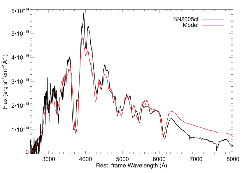
Figure 1: Synthetic spectrum from our ejecta model (red line) compared to an observed UV-optical spectrum (black line) taken 0.9 days before $B$ maximum (Bufano et al. 2009; Garavini et al. 2007).

All synthetic spectra in this paper are derived from a model developed for SN 2005cf, for which UV/optical data near maximum is available (Bufano et al. 2009; Garavini et al. 2007; Wang et al. 2009). SN 2005cf was a bright supernova ($M_{B}=-19.39$ (Pastorello et al. 2007)) with a light-curve width $\Delta m_{15}=1.10$ (Pastorello et al. 2007; Wang et al. 2009) which corresponds to a light-curve stretch of $s=0.93$ using the relation in Conley et al. (2008). Since SN 2005cf was a bright SN and produced a large amount of ⁵⁶Ni ($\approx 0.7M_{\odot}$) we chose to use as the density structure of model WDD3 from Iwamoto et al. (1999). The bolometric luminosity of this model is $\log(L_{bol}/L_{\odot})=9.6$.

We have used an abundance tomography approach to model the UVOIR spectrum of SN 2005cf 0.9 days before maximum. The method of successively constraining the abundances in deeper and deeper layers using a temporal sequence of spectra was first introduced by Stehle et al. (2005). In order to constrain properly the highest velocity material in the outermost ejecta before trying to model a spectrum at maximum, we started with a spectrum obtained $-7.8$ days before $B$-band maximum. The maximum brightness spectrum has a phase of $-0.9$ days relative to $B$-band maximum. We assume a B-band rise-time of $19.5$ days (Conley et al. 2006) and use $t=18.6$ days. In order to optimise the fits to the data, two additional zones were introduced on top of those at maximum and pre-maximum velocities, as in Sauer et al. (2008). This is not unexpected as strong high-velocity features have been noted in SN 2005cf (Garavini et al. 2007). We optimised the match to the UV spectrum ($\lambda<4000$ Å) while maintaining the best possible fit in the optical.

This model is reproduced in Figure 1. A summary of the chemical composition in each zone is given in Table 1 where IME stands for intermediate mass elements (those with atomic number 9 – 20) and IGE for iron-group elements (atomic number greater than 20).

From Table 1 we see that the outer two layers are dominated by unburnt carbon and oxygen with very little IME and almost no IGE. In the pre-maximum layer, there is still some C/O material remaining and slightly more IGE material, but the shell is dominated by material that has been burnt to IME. The shell at the photospheric velocity at maximum is still dominated by IME, but now a significant fraction of the shell is made up of IGE.

Table 1: A summary of the major element groups in each shell of the model for SN 2005cf. X is the mass fraction of C/O, intermediate mass elements (IME) and iron group elements (IGE).

Zone	$v_{\textrm{ph}}$	$v_{\textrm{pre-max}}$	$v_{\textrm{out,1}}$	$v_{\textrm{out,2}}$
Velocity	10750	13100	16000	19500
X(C/O)	0.3	4.0	70	92
X(IME)	63	92	18	8.2
X(IGE)	37	3.9	3.2	0.2

We used this technique to create models for supernovae with different bolometric luminosities. The range of luminosities was chosen to reflect the spread of observed SN Ia properties. We also used different underlying density profiles to reflect the different energies and ⁵⁶Ni production at the bolometric luminosities $\log(L_{bol}/L_{\odot})=9.2,9.4,9.6,9.75$. The velocities of the $v_{\textrm{ph}}$ and $v_{\textrm{pre-max}}$ shells move depending on luminosity (Table 2), resulting in the masses of individual elements being scaled for the whole model. However, within each shell the relative abundances of the SN 2005cf model are preserved as described. In order to ensure that we produce realistic models, we compare the model output spectrum to observed SNe Ia to ensure we are producing spectra which match the continuum levels in the UV while maintaining normal optical spectra i. e.  are not members of the over-luminous of under-luminous subclasses. This process is summarised in Table 2 and the spectra are displayed in Figure 2

Table 2: An overview of the model parameters for the models $\log(L_{bol}/\L_{\odot})=\textrm{9.2, 9.4, 9.6, 9.75}$ with $\eta=1$. The W7 model is from Nomoto et al. (1984) and the WDD1 and WDD3 models are from (Iwamoto et al. 1999). The given velocities are in  km s^-1.

	9.2	9.4	9.6	9.75
Density Structure	W7	WDD1	WDD3	WDD3
$v_{\textrm{ph}}$	6783	8539	10750	11250
$v_{\textrm{pre-max}}$	8366	10406	13100	13710
$v_{\textrm{out,1}}$	16000
$v_{\textrm{out,2}}$	19500

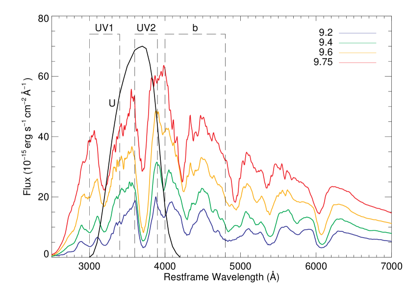
Figure 2: The $\eta=1$ spectra for $\log(L_{bol}/L_{\odot})=\textrm{9.2, 9.4, 9.6, 9.75}$. Also marked are the three top-hat filters introduced in E08, UV1, UV2 and b (dashed lines) and the Bessel U filter (solid black line).

We then used these 4 luminosity bins to create a set of models with varying metal contents. We do this by scaling the metallicity in the pre-maximum and two outer shells with respect to the best-fitting model: the photospheric shell remains unchanged. To generate the sequences, we multiplied the abundances of all the elements with atomic number $Z>20$, i. e. heavier than calcium, by a factor $\eta$, which is allowed to take the values $\eta=0.05,0.1,0.2,0.5,1,2,5$. The mass fraction $X$ of element $E$ thus becomes $X(E)=\eta X(E)_{0}$ where $X(E)_{0}$ is the mass fraction of the element in the SN 2005cf best-fit model at the expense of unburnt C/O. This provides us with a grid of $4\times 7$ models for our analysis, but we have excluded the model where $\log(L_{bol}/L_{\odot})=\textrm{9.75}$ and $\eta=0.05$ as the optical spectrum did not look normal, leaving 27 models for analysis. A metallicity sequence is shown in Figure 3 for $\log(L_{bol}/L_{\odot})=\textrm{9.6}$. For all values of $\eta$, the optical spectra appear normal with relatively little dispersion. However, in the UV the dispersion between the models increases dramatically and diversity is also seen in the shapes and positions of features. This reflects the fact that metal line-blanketing effect is stronger in the UV.

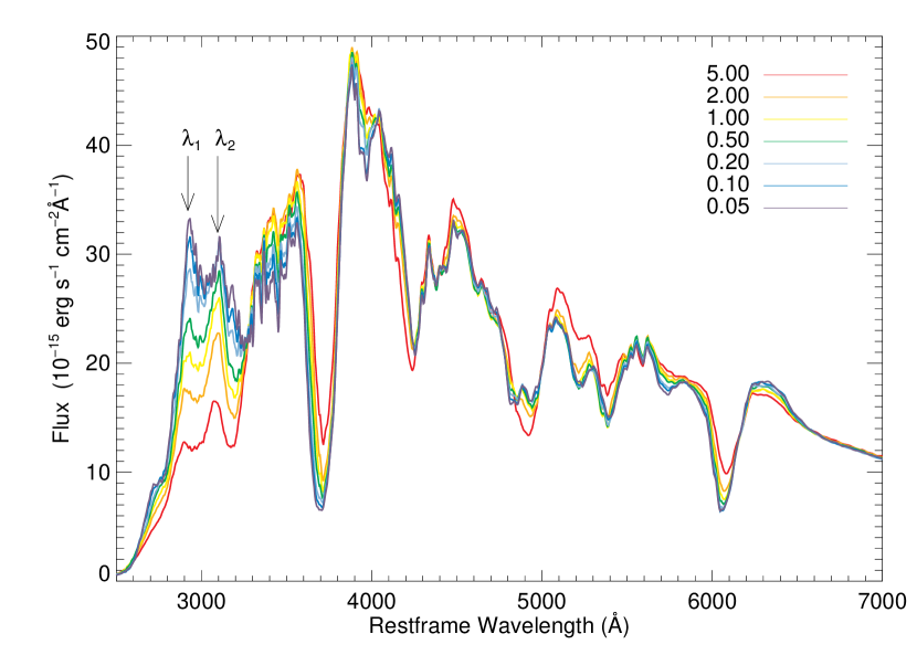
Figure 3: The $\eta=5,2,1,0.5,0.2,0.1,0.05$ spectra for $\log(L_{bol}/L_{\odot})=\textrm{9.6}$. The features $\lambda_{1}$ and $\lambda_{2}$ are also marked.

One caveat with our models is that in the red and infrared the fits to data are less good. This is because of the crude assumption of a blackbody at the photosphere. The flux inside an SN Ia is non-thermal even in the inner layers (see Sauer et al. 2006). Flux redistribution within the inner parts of the simulated atmosphere leads to a sufficiently accurate radiation field in the atmosphere in the ultraviolet and blue regions of the spectrum, but in the red and infrared some flux excess usually remains in the synthetic spectra with respect to observations. This can be seen in Figure 1 where the model flux is higher than the observed flux from $\approx 6300$ Å onwards. This means that our estimates of $L_{Bol}$ may be somewhat larger than the real value when the red and IR are overestimated. Therefore, in order to compare models and data we extract $L_{B}$ from both.

2.2 Observational Data

The observational data for this study are taken from those presented in E08. These SNe were discovered as part of the Supernova Legacy Survey (SNLS, Sullivan et al. 2011), a real-time Type Ia supernova search based at the Canada-France-Hawaii Telescope (CFHT) which used $g^{\prime}r^{\prime}i^{\prime}z^{\prime}$-band observations to identify high-z SNe Ia. For more details on the real-time SNLS target selection pipe-line see Perrett et al. (2010).

E08 observed a selection of SNLS supernovae on the Keck I Telescope, using LRIS (Oke et al. 1995) to obtain a high signal-to-noise ratio in the rest-frame UV. Using host photometry obtained from the deep stack CFHT images in the $u^{*}g^{\prime}r^{\prime}i^{\prime}z^{\prime}$-bands, a best-fitting template galaxy spectrum was used to remove contamination from host galaxy light in the SN spectrum. For more details on this see E08, or Walker et al. (2011) which gives a detailed explanation of the application of this method to SNLS data obtained at the Gemini and VLT telescopes.

It is important to note that while the sample of supernovae used in E08 as a whole was representative of the supernova population, the sub-sample of these spectra we use here are not because we apply a cut for rest-frame phase. In this study, in order to make a realistic comparison of models to data, we included only supernovae with a rest-frame phase of $\pm 3$ days from $B$-band maximum. Additionally, we only considered ”normal” SNe Ia with good lightcurve coverage so the $B$-band maximum magnitude could be calculated, and with a spectrum reaching a minimum rest-frame wavelength of $\leq 2700$Å. These cuts leave 9 objects.

Within our sub-sample the mean light-curve stretch is $\overline{s}=1.08$, where 1.0 represents the fiducial ”normal” SN Ia lightcurve. In fact, within our sub-sample, all but one of the objects have a stretch value $>1$. The mean colour of our subsample is $\overline{c}=-0.027$. The light-curve fitting was carried out using the SiFTO fitter (Conley et al. 2008). SiFTO also fits a $B$-band magnitude at maximum. To obtain $L_{B}$ we convert magnitude to flux and then to luminosity assuming a flat cosmology with $\Omega_{M}=0.269$ (Sullivan et al. 2011) and $H_{0}=70$ km s^-1 Mpc^-1.

In Figure 4 we plot the various models at $\log(L_{bol}/L_{\odot})=\textrm{9.6, 9.75}$ and compare them to our observational data assuming all supernovae are placed at 10 pc. The variations in metallicity appear to match the variations in the spectra of the E08 sample. The spectrum lying below the models and the other observed SNe Ia with $\log(L_{bol}/L_{\odot})=\textrm{9.6}$ is 04D1sk. This appears to have a low UV flux compared to the optical. As such, we expect this to be an outlier in some of our UV colour analysis (Section 3.1). None of the observed supernovae have luminosities which would correspond to the $\log(L_{bol}/L_{\odot})=\textrm{9.2,9.4}$ models; however SNe Ia are observed to have luminosities in this range (see Figure 11 for example).

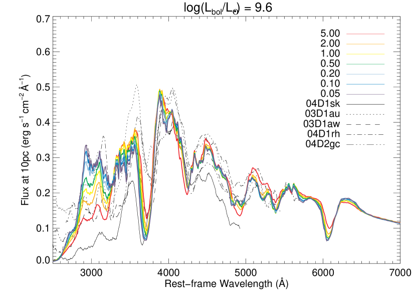
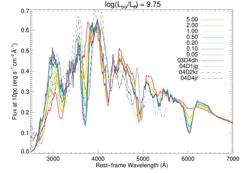
Figure 4: For all values of $\eta$, the models with $\log(L_{bol}/L_{\odot})=\textrm{9.6}$ (top) and $\log(L_{bol}/L_{\odot})=\textrm{9.75}$ (bottom) are compared to observed spectra from E08.

3 Analysis

We now have a set of models and observed spectra which can be analysed in identical ways. As the $B$-band magnitudes of the observed supernovae are well-known from their use in cosmology, we revert to using the $B$-band luminosity $L_{B}$ instead of bolometric luminosity as this quantity is measureable for both the models and observed supernovae. We can therefore make direct comparisons between the observed and model data for the UV diagnostics described in this section. It is possible to see from later plots that at constant $L_{bol}$, $L_{B}$ does not vary linearly with $\eta$.

3.1 UV Colours

We first examine the broadband UV colours at maximum light as first examined in E08. Their study used Bessel U filter as well as three top-hat filters they defined in the UV and optical (UV1, UV2 and a normalisation filter b; see Figure 2). We do not perform any correction for supernova colour and remeasure the U, UV1, UV2, b magnitudes for the models and the observed spectra. The results are plotted in Figure 5.

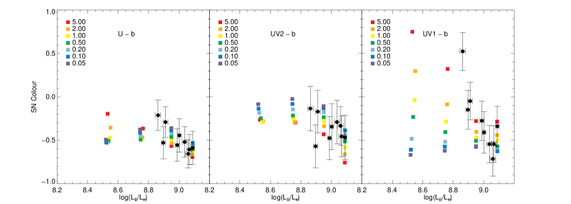
Figure 5: UV colours for the models and the data. The models are shown as the coloured squares and the data in the black filled circles.

This shows that the broad trends observed within the E08 data at maximum are replicated in the models. The filters U and UV2 do not show any strong trend with colour and $B$-band luminosity. The dispersion between models of different metallicity is small, and the trend between metallicity and colour is not always linear. The UV1 filter shows that for the higher metallicity models the UV colour can be large for supernovae with lower luminosities. In general, the dispersion in the UV1 filter, which is the bluest of the three, is the largest. Given the smaller dispersion in the models and the large errors in the data, it is not possible to attribute the change in colour to metallicity, although this may become possible with more, better data. In the UV1 filter, the evidence that our less luminous SNe come from regions of higher metal content is stronger.

As predicted above, 04D1sk is the reddest object for all three colours. It appears particularly red in the UV1-b bands implying that its ejecta are particularly metal-rich.

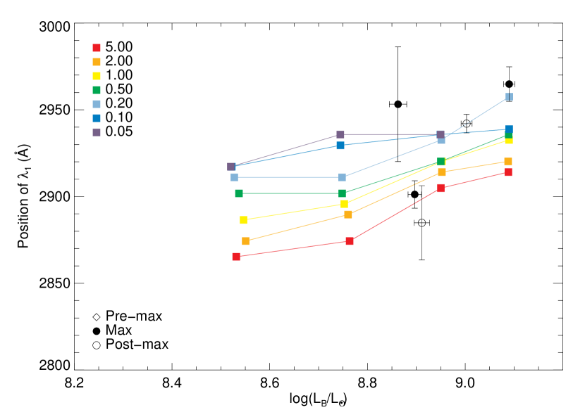
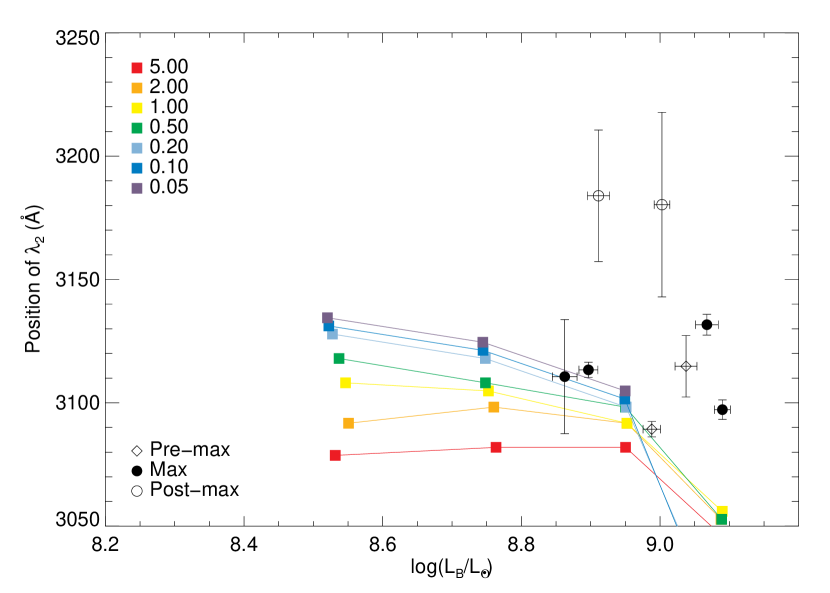
Figure 6: The UV emission features $\lambda_{1}$ (left) and $\lambda_{2}$ (right) from E08 plotted against $B$-band luminosity for both observed data and values measured from the models. The different colours denote the different metallicities in the model spectra. The observed data is divided into sub-samples based on the rest-frame phase of the spectra

3.2 UV Emission Feature Diagnostics

Another property examined by E08 is the position of two UV features described as $\lambda_{1}$ and $\lambda_{2}$ positioned at $\approx 2900$Å and $\approx 3100$Å respectively. The variation of these peaks with metallicity can clearly be seen in our models in Figure 3. The reason for this shift can simply be found in the fact that if the metal content is higher lines are effective at higher velocities, and hence absorb at bluer wavelengths, progressively shifting the reemission peaks towards the blue.

We use the same Gaussian-fitting method as described in E08 to measure the positions of $\lambda_{1}$ and $\lambda_{2}$ in the model data as well for the observed spectra, although we first apply some smoothing to the observed data. As we only have model spectra at one phase (maximum) we choose to further sub-divide this sample due to the steep observed time-dependence of the position of these features (E08). These comparisons are shown in Figure 6 where instead of plotting $\lambda_{1}$ or $\lambda_{2}$ against phase, we plot them against $L_{B}$. The observed data are divided as $-3\leq\mathrm{phase}<1$ days (pre-max; open diamond); $-1\leq\mathrm{phase}<1$ days (max; filled circle); $1\leq\mathrm{phase}\leq 3$ days (post-max; open circle).

From the left plot in Figure 6 we see that at higher luminosities there is a lower dispersion in the values of $\lambda_{1}$ in the models. The models show that $\lambda_{1}$ is roughly constant with luminosity in the lower metallicity models. We also see an approximately constant value of $\lambda_{1}$ within the observed data for all but 2 of the spectra with no strong phase-dependence.

Figure 6 (right plot) shows that the position of the synthetic $\lambda_{2}$ peak emission varies strongly with both luminosity and metallicity (see above). The observed data at $\pm 1$ day agrees with the measurement in the models and the strong phase-dependence of the position of this feature is observed. At the highest luminosity, the position of the feature is strongly blueshifted out of the range of measurements found by E08. This is because these features are strongly affected by the supernova velocities (see below) and at the highest luminosities the widths of $\lambda_{1}$ and $\lambda_{2}$ are very broad. This causes the two peaks to merge making the identification of $\lambda_{2}$ difficult as the features are not Gaussian in nature (see Figures 2 and 3).

3.3 UV Flux Ratio

We can use our data to measure the UV flux ratio of Foley et al. (2008), $R_{UV}$, which is defined as

$$R_{UV}=\frac{f_{\lambda}(2770\textrm{\AA})}{f_{\lambda}(2900\textrm{\AA})}$$ (1)

where $f_{\lambda}(2770\textrm{\AA})$ and $f_{\lambda}(2900\textrm{\AA})$ are the median fluxes in bands of size $\pm 20$ Å centred at these wavelengths. The results are plotted in Figure 7.

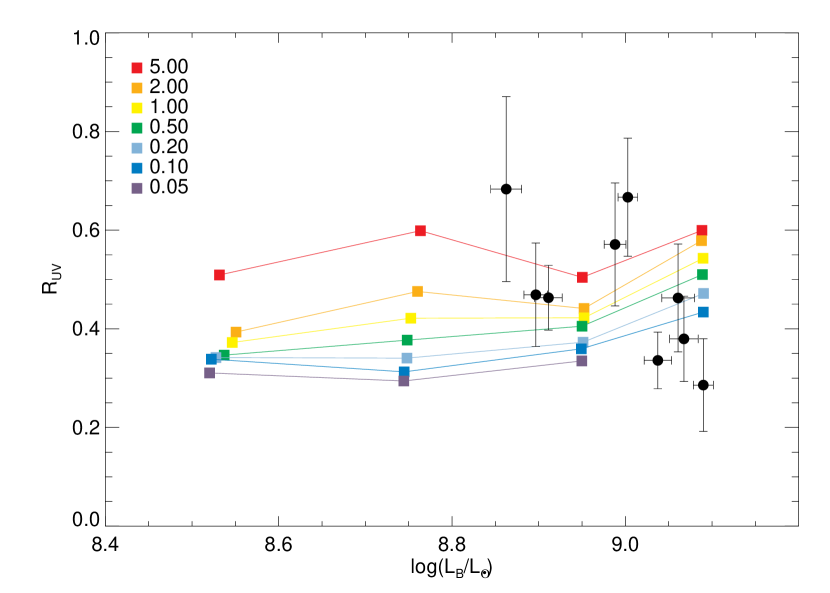
Figure 7: The measured $R_{UV}$ for both models and observed data. The different colours represent the different values of $\eta$ for a given luminosity.

Figure 7 shows that for a given metallicity ($\eta$), the value of $R_{UV}$ is approximately constant. The model trends agree broadly with the values of $R_{UV}$ measured from the observational data, but in this region of the spectrum the observed data is strongly affected by noise. We could only reproduce the correlation between $L_{B}$ and $R_{UV}$ as would be expected from the results in Foley et al. (2008) if the brighter observed SNe Ia are in more metal-rich hosts. Instead the models show that the diversity is driven almost entirely by the difference in metallicity. Some trend in seen in the data and the strength of this correlation is $2.4\sigma$ using a Spearman’s Rank correlation statistic assuming all points are equally weighted. We do not conclude anything from this because of the small sample size.

We have also performed an analysis of $R_{UV}$ after performing a colour-correction to the supernovae using the SALT2 colour law (Guy et al. 2007). The change in the measured value of the ratio with this correction in the order of 0.005 and so much less than the $1\sigma$ error on the $R_{UV}$ measurement based on the noise of the data. We have also examined what would happen should the host subtraction of the galaxy as described in E08 be incorrect. We found that addition/subtraction of any galaxy template used in E08 with a $u^{*}$-band flux of up to 20% that of the supernova would not change the $R_{UV}$ measurement by more than the $1\sigma$ error. As such we do not believe our $R_{UV}$ measurements would be strongly affected by any inaccuracies in the host subtraction.

4 Discussion

4.1 UV Colours

We broadly replicate the wide range of colours observed in the UV with our models. We also show that dispersion increases towards the blue. This is due to the increasing extent of the metal line-blanketing which affects the whole of the UV region reflected in the opacity of the SN ejecta increasing by 3 orders of magnitude from 4000Å to 2000Å (Sauer et al. 2006). This increase in dispersion is also consistent with the SWIFT data results Brown et al. (2010)

The UV colours are the best diagnostic we have featured for replicating properties seen by the whole observed data sample. This is because they measure over wide wavelength ranges and so are less affected by variations caused by the velocities in the models not matching the high-z data precisely.

4.2 UV Peaks

The two features designated as $\lambda_{1}$ and $\lambda_{2}$ in E08 are not emission features in the traditional sense. The sheer number of species absorbing in these regions makes this extremely unlikely. The reason for the peaks in flux at $\approx 2900$ Å and $\approx 3100$ Å could be due to two things, or most likely a combination of both: a ”window” in opacity at these wavelengths which allows more of the photons emitted from the photosphere to escape, or reverse fluorescence from species in the outer layers of the ejecta are generating these blue photons (Mazzali 2000). We can use the output of the model code to investigate what happens to photon packets emitted from the photosphere to try and differentiate between the two.

Firstly, we look at what happens to packets emitted from the photosphere in a region of $\pm 40$ Å around the wavelengths of the measured values of $\lambda_{1}$ and $\lambda_{2}$. We find that at these wavelengths, for both features and at all luminosities and metallicities, between 50% – 80% of the packets are reabsorbed back into the photosphere through backscattering. Of the small number of packets left, they are mostly re-emitted at redder wavelengths. This means that an opacity window at low velocities can be excluded as the dominant effect.

We can also look at photon packets which were originally emitted in other regions of the spectrum, absorbed in some line transition and finally re-emitted within the $\lambda_{1}$ and $\lambda_{2}$ regions. This is illustrated in Figure 8. We see here that for $\lambda_{1}$ by far the most packets are gained from the red in reverse fluorescence processes, although this percentage decreases as luminosity increases. The situation is similar for the $\lambda_{2}$ feature, although by the time we reach our highest luminosity model, the percentage is roughly 50% from the blue and 50% from the red. Reverse fluorescence was already mentioned as being primarily responsible for the emerging UV flux by Mazzali (2000): photons are fluoresced back to the UV at high velocities, and thus they can escape in low-oacity environments.

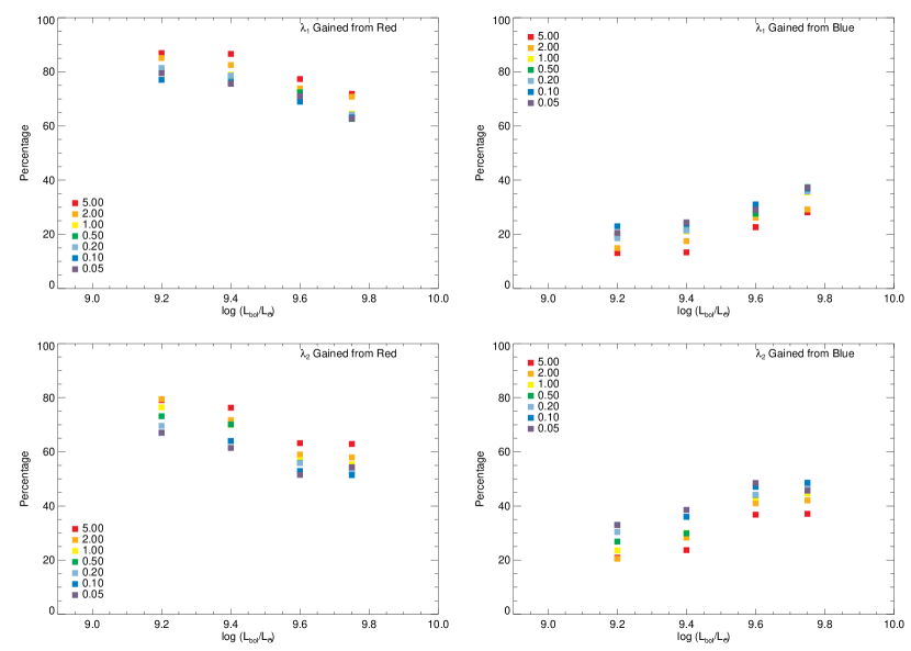
Figure 8: The percentage of packets gained in the $\lambda_{1}$ (top) and $\lambda_{2}$ (bottom) regions which were originally emitted at redder (left) or bluer (right) wavelengths.

If we also look at this measurement in terms of the number of packets gained rather than the percentage of packets, we actually see that for both features the number gained from the blue increases with luminosity, which is to be expected because of the increase in temperature. The number of packets gained via reverse fluorescence, meanwhile, does not increase in the same way. For $\lambda_{2}$ the number increases in the lower two models and after that remains constant meaning that the lines in the optical have become saturated and this is limiting the number of photons re-emitted in this region. The number of packets for $\lambda_{1}$ does not saturate and so this is still affected by the abundances of the IME and IGE which absorb photons in the optical.

We can also examine which ions cause the processes that shift flux into the $\lambda_{1}$ and $\lambda_{2}$ regions. We find that for both features, the predominant species which reverse fluoresce are IME, particularly Mg ii, Si ii and S ii, with some contributions from the Fe-group elements, notably Cr ii. As these features are dependent on abundances of elements they will be affected by any differences between the velocity structure and the abundance stratification between the models and the data. This can account for some of the discrepancy we see between the positions of the features.

4.3 UV Ratio

It has been established that a source of UV flux is a process of reverse fluorescence where red photons are absorbed and re-emitted at shorter wavelengths at high velocties (Mazzali 2000). This means that there have to be some metals in the material above the photosphere or there would be no UV flux at all. As the metal content is increased, the UV flux increases due to an increasing amount of reverse fluorescence; however this is in competition with an increased absorption of the UV photons by the metals themselves. The way this occurs in the regions of $f(2770)$ and $f(2900)$ determines how $R_{UV}$ changes with metallicity at constant luminosity.

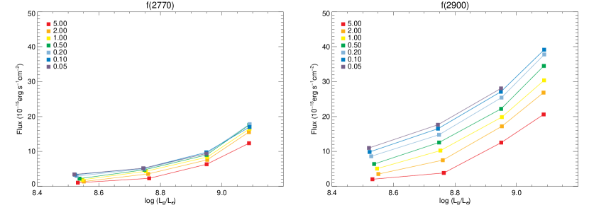
Figure 9: Median flux values in the two regions probed by $R_{UV}$ for our model $(L,\eta)$ sequences.

We have plotted the values $f(2770)$ and $f(2900)$ in our models in Figure 9. In all cases, we see that the higher $\eta$ models have less flux as there are more metals absorbing in these bands. In both bands we see a dispersion with metal content, which is larger for $f(2900)$. This shows that the variation in $R_{UV}$ is driven more by the variation in the $f(2900)$ band.

We used the MC code to identify the dominant absorption lines in the regions probed by $R_{UV}$ looking at ions with a large absolute change in absorption strength between $\eta=0.05$ and $\eta=5$ (Table 3) or ions which have large mean absorption strengths averaged over the metallicity sequence (Table 4). We can do this analysis for $R_{UV}$ because of the small wavelength ranges for $f(2770)$ and $f(2900)$. No single element appears to be responsible for the change, although the $f(2900)$ region appears to be dominated by variations in the Cr ii lines. We see that in the higher luminosity models, the dominant species change from singly-ionised to doubly-ionised reflecting the increase in temperature in the atmosphere. Figure 9 explicitly shows that effect of varying $\eta$ has on the two spectral bands.

Table 3: The species which show the largest absolute change in line strengths with metallicity in the two regions probed by $R_{UV}$.

$\log(L/L_{\odot})$	$f(2770)$ Region	$f(2900)$ Region
9.2	Fe ii	Cr ii
9.4	Fe ii	Cr ii
9.6	Singly-ionised metals	Cr ii
9.75	Doubly-ionised metals	Cr ii

Table 4: The species which show the largest mean line strengths across all metallicities in the two regions probed by $R_{UV}$. “–” marks mean that the region contains a mix of singly- and doubly-ionised species of a variety of elements.

$\log(L/L_{\odot})$	$f(2770)$ Region	$f(2900)$ Region
9.2	Fe ii	Singly-ionised metals
9.4	Fe ii	Singly-ionised metals
9.6	Singly-ionised metals	–
9.75	Doubly-ionised metals	Doubly-ionised metals

4.4 Focus on Individual Elements

As well as creating sequences of models where the multiplier $\eta$ affects all elements with $Z>20$, we can use $\eta$ to vary one element while keeping all others fixed. This allows us to examine whether this one element is the cause of any of the observed effects we see. Should any of this be caused by one element alone this would give us an important diagnostic to examine the physics of the supernova explosion itself. The species for which this analysis was carried out are chromium, stable iron, manganese, ⁵⁶Ni and titanium which are the elements with species with the strongest features in the near-UV. We summarise the effect of individual elements below:

• UV Colours: Ti and Mn have no effect on the UV colours. Stable iron has little effect, except in the UV1-b colour where it shows strong non-linear trends with iron content at a given luminosity. The chromium and ⁵⁶Ni model sequences both show a large dispersion in the UV1-b colour as seen for all metals in Figure 5 above.
  

• UV Features: The position of $\lambda_{1}$ is strongly dependent on the increased amount of Cr in the spectrum. This is expected from looking at which elements have caused the reverse fluorescence in this feature. The position of $\lambda_{2}$ is affected by the IGE produced in nucleosynthesis i. e.  iron, nickel and chromium, but not manganese. We see that these IGE are small contributors to the reverse fluorescence flux which is dominated by IME, so $\lambda_{1}$ and $\lambda_{2}$ will be very sensitive to small changes in the relative abundances of all these elements.
  

• UV Ratio: The sequences with varying stable iron and chromium content from nucleosynthesis all show large variations at constant luminosity. This is expected as their ions were identified in Tables 3 and 4. There is diversity shown for all of the element sequences although to a lesser degree. This implies that this feature could vary significantly between supernovae and be dependent on velocity (which absorptions are shifted into the bands); temperature or luminosity affecting ionisation balanaces; and the abundances of the individual elements relative to each other which may not be the same as for SN 2005cf.

The plots detailing these results can be found in the Appendix.

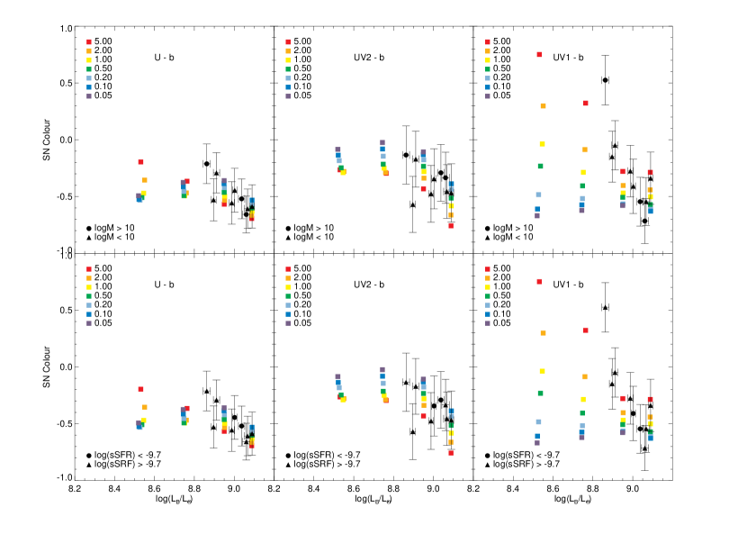
Figure 10: UV colours in the models and the observed spectra with the observed objects from E08 divided into two sub-samples based on their host mass (top) and the host specific star formation rate (bottom). The values of the specific star formation rate (sSFR) are from Sullivan et al. (2010). The model sequences for different values of the metal content in the SN outer layers ($\eta$) are again plotted in different colours.

4.5 Links to Other Observables

4.5.1 Host Metallicity

It is not possible to use our models to explain directly the observed trends with host properties. This is because our method of generating spectra does not separate out the effect of an increased metal content in the outer layers of the SN ejecta due to progenitor or environmental metallicity from any potential upmixing of elements which are burnt during the SN explosion.

Hints on whether the environmental metallicity plays a major role for the UV colours may directly be obtained from the observations by subdividing the observed sample according to metallicity indicators. In Figure 10, we have done this, with the host galaxy mass and its specific star formation rate, sSFR, as measured in Sullivan et al. (2010) as indicators. More massive galaxies with lower star-formation rates should generally be old, red ellipticals which have a high metallicity. In the upper panel of Figure 10, there are two SNe in massive (high-metallicity) galaxies which are found to have low-$R_{UV}$ / high-luminosity; however, there is also one SN in a high-mass host which shows an inverse tendency so we do not see any trend with host mass. Using the sSFR as a criterion (Figure 10, lower panel), we see a similar result. Fr

4.5.2 Supernova Light-curve Standardisation

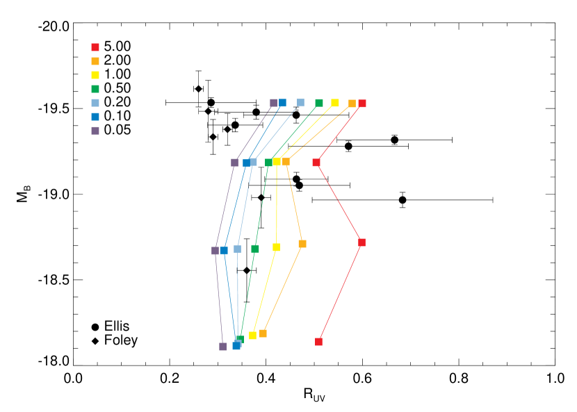
Figure 11: $B$-band magnitudes plotted against $R_{UV}$ for the models in this paper and objects investigated in Foley et al. (2008) and E08. No correction for light-curve shape or colour has been made to the data.

Foley et al. (2008) proposed that an observed correlation between $R_{UV}$ and the $V$-band magnitude could be used for standardisation of supernova magnitudes. In Figure 11, we extend this into the $B$-band and compare the supernovae in that sample to those from E08 and our models, where the values of $M_{B}$ from the models are generated via synthetic photometry. For the Foley et al. (2008) data, the $B$-band magnitudes are taken from Altavilla et al. (2004). The low-z data includes the measurement of $R_{UV}$ nearest to maximum for SN 1980N, SN 1981B, SN 1990N, SN 1991T and SN 1992A. Figure 11 shows that within the luminosity region populated by SNe Ia which obey the Phillips relation the E08 data do not confirm the linear correlation suggested in Foley et al. (2008). The range and scatter of $R_{UV}$ measurements of the E08 sample appear to have more in common with the supernovae in the more recent Foley et al. (2012) study which uses $M_{V}$ so cannot be directly compared to these values.

A larger sample of well-observed SNe may be needed to clarify this disagreement. In any case, $R_{UV}$ is a flux ratio, not a broad-band colour measurement, so it is very sensitive to slight changes in the UV spectrum, which can be caused not only by different abundances in the ejecta, but also by small shifts in velocity. At 2770Å, a change of 20Å is equivalent to a change in velocity of $\approx 2000$ km s^-1. This is velocity change which could quite easily occur in normal SNe Ia. The measurements will also be strongly influence by the phase of the supernova as we can expect velocity shifts as observed in the optical. The phase-dependence of the $\lambda_{2}$ is shown in Figure 6.

The best opportunity to use the UV for light curve calibration is the strong trend between $L_{B}$ and the (UV1 - b) colour as shown in Figure 5. The b filter corresponds to the optical region where supernovae are less susceptible to metallicity differences, and the features maintain a constant morphology despite differences in flux. Figure 5 shows that for the same luminosity the UV changes dramatically with metallicity, while $L_{B}$ is basically constant.

The UV1 region changes dramatically with both luminosity and metallicity which drives the trend seen Figure 5. It is possible that with optimisation, this colour could be used for lightcurve standardisation. (U-b) also shows a linear trend in the observed data as the U filter extends down as far as 3000Å, but at lower luminosity the models show the trend is not monotonic with metallicity. This would make any standardisation difficult.

4.6 Future Extensions of This Study

The observational data used in this paper are subject to large errors in both luminosity and $R_{UV}$. New observations with higher S/N in the UV would reduce the errors on $R_{UV}$. Observations of supernovae with lower luminosities would also enable a thorough comparison with the model data in these ranges.

In terms of the modelling, we have used only one well-studied supernova as the basis of our models. While our spectra appear normal at a variety of luminosities and metallicities, they are artificial in having been produced by arbitrary changes to the input parameters. With more well-studied supernovae with UV data, we would have more starting points for the creation of more accurate models covering a wider range of initial luminosities. This may then help to produce more accurate replicas of observed supernovae and reduce some of the disagreement seen between the models and the data. Velocity changes particularly affect the single feature and narrow-band measurements so sets of models which explore different parts of this parameter space would be especially helpful here.

In the future it may also be possible to do a similar analysis for pre-maximum spectra where spectral signatures of the unburnt material from the progenitor are more easily identified in the optical.

5 Conclusions

We have used maximum-light spectra for a sample of 9 SNe Ia obtained by E08 and compared them to a series of 1D models produced by a MC radiative transfer code in order to test whether the variations observed the UV region of the spectrum can be explained by metallicity and luminosity changes alone. Our model spectra were initially based on one-well observed example SN 2005cf. We summarise our conclusions in the following points

• Our models replicate well the range of broad-band UV colours seen in the observed spectra, showing that the dispersion increases as one progresses to shorted wavelengths. The (UV1-b) colour appears to depend strongly on metallicity, and it might have the potential for use in light-curve standardisation because it is less sensitive to very small changes in absorption features than narrow-band indicators(Sections 4.1 and 4.5.2); however this requires further observational data for testing at lower luminosities.

• We observe that $\lambda_{1}$ and $\lambda_{2}$ can be interpreted as peaks caused by the reverse fluorescence of photons into the UV region of the spectrum, mainly from intermediate mass elements and chromium (Section 4.2). Both $\lambda_{1}$ and $\lambda_{2}$ move towards the blue with increasing metal content in the upper layers of the ejecta, but the effect is highly non-linear and may not be the best metallicity indicator.

• We see that $R_{UV}$ in our models has a low dependence on luminosity and the effect of the metal content is complex (Section 4.3). High-z data do not confirm the relation of Foley et al. (2008), and so we do not support using this index for light curve standardization.

• We have used high-z Type Ia supernovae spectra from (E08) and measured observed values of $R_{UV}$ for 9 objects around maximum light. We see that the measured values agree with those in the models, although they are affected by large errors from noise in the spectra (Figure 7).

• We have performed an extensive search using the model spectra in order to investigate the possibility that these results are driven by one or two elemental transitions, but the results have shown that the UV spectrum is far too complicated for this. In light of this we suggest that the use of $R_{UV}$ is not appropriate for light-curve standardisation as the trends with metallicity and absolute magnitude are not linear (Section 4.4).

Appendix A Single Element Sequences

Figures 12 – 16 show the effect that changing the amount of only 1 element has on the UV colours, positions of the UV emission features and the ratio $R_{UV}$.

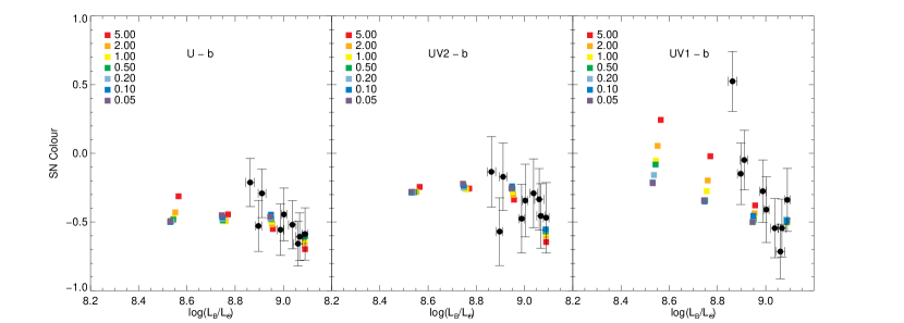
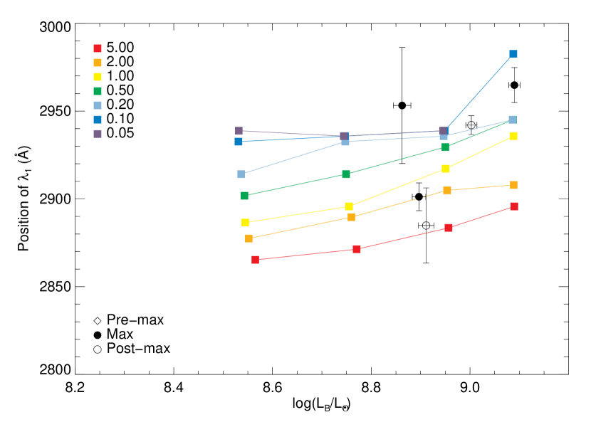
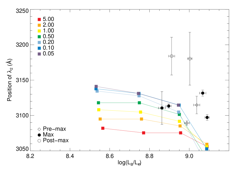
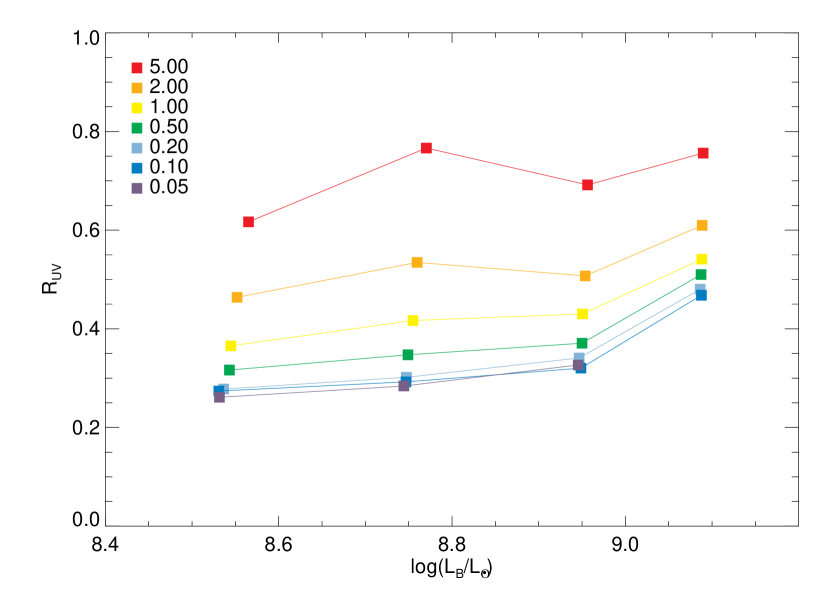
Figure 12: The effect of changing just the amount of chromium in the outer ejecta. Upper – UV colours; Middle – The positions of $\lambda_{1}$ and $\lambda_{2}$; Lower: $R_{UV}$

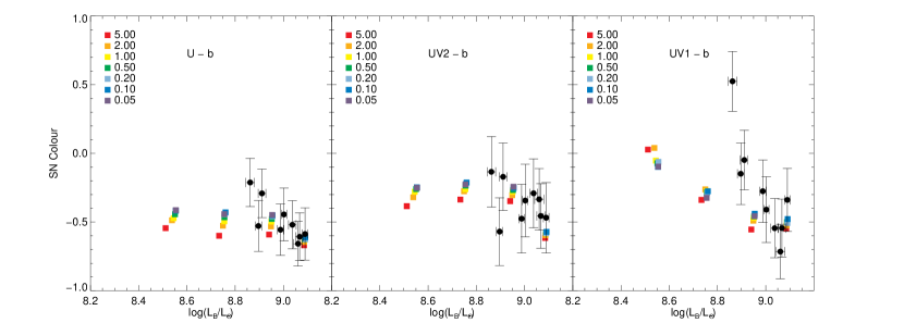
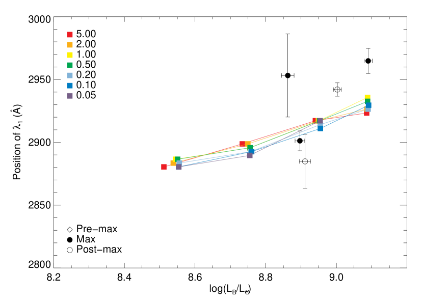
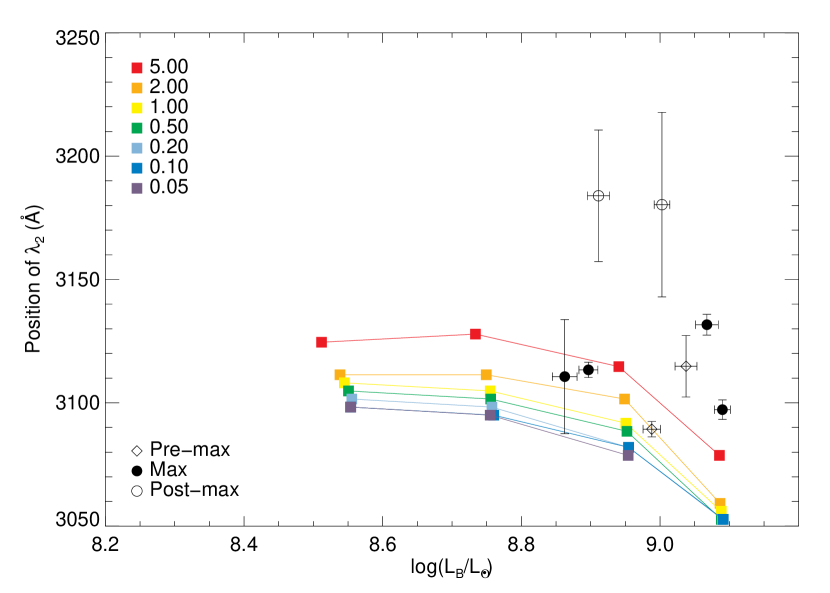
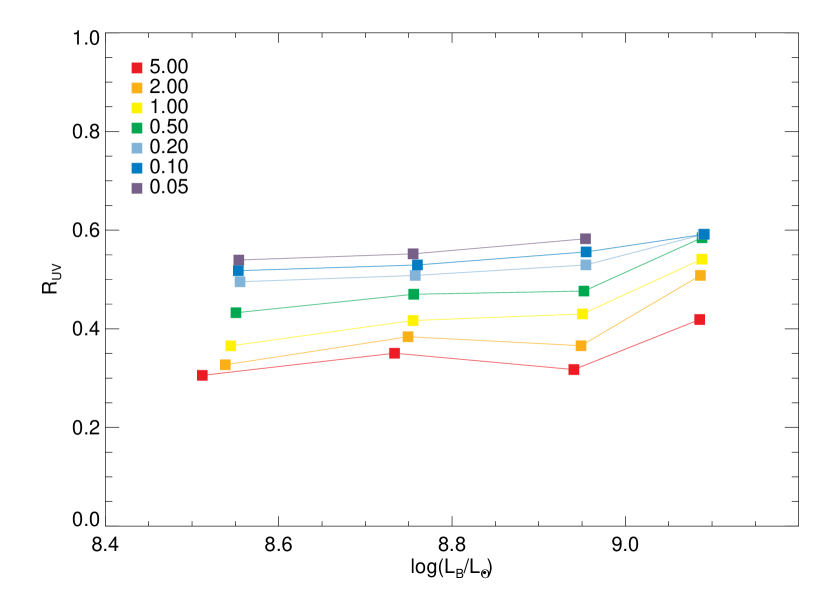
Figure 13: The effect of changing just the amount of stable iron in the outer ejecta. Upper – UV colours; Middle – The positions of $\lambda_{1}$ and $\lambda_{2}$; Lower: $R_{UV}$

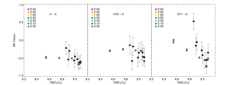
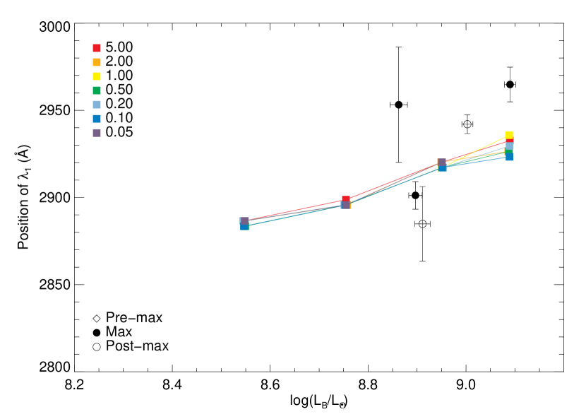
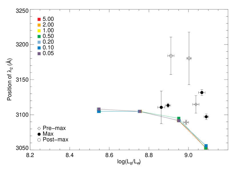
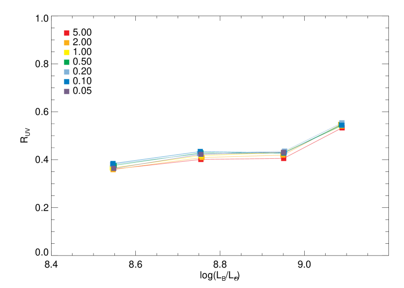
Figure 14: The effect of changing just the amount of manganese in the outer ejecta. Upper – UV colours; Middle – The positions of $\lambda_{1}$ and $\lambda_{2}$; Lower: $R_{UV}$

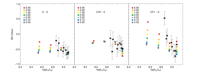
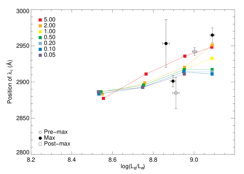
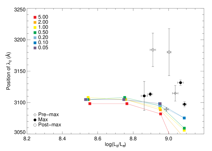
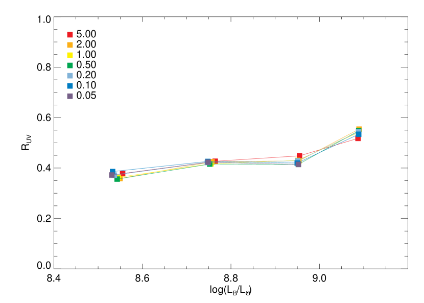
Figure 15: The effect of changing just the amount of ⁵⁶Ni in the outer ejecta. Upper – UV colours; Middle – The positions of $\lambda_{1}$ and $\lambda_{2}$; Lower: $R_{UV}$

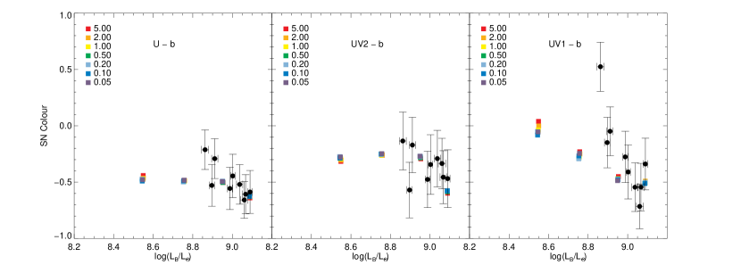
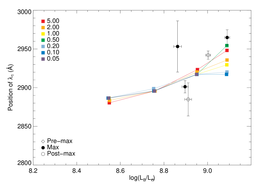
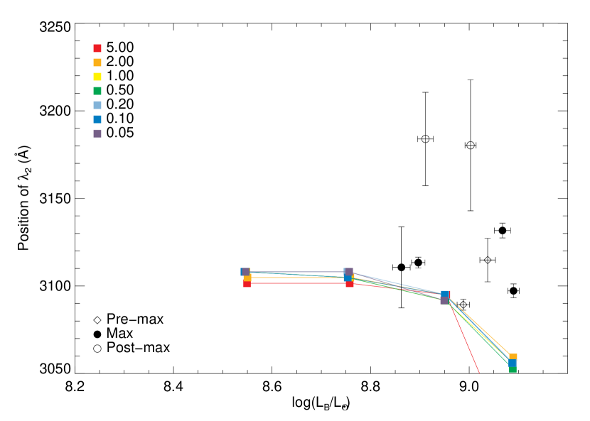
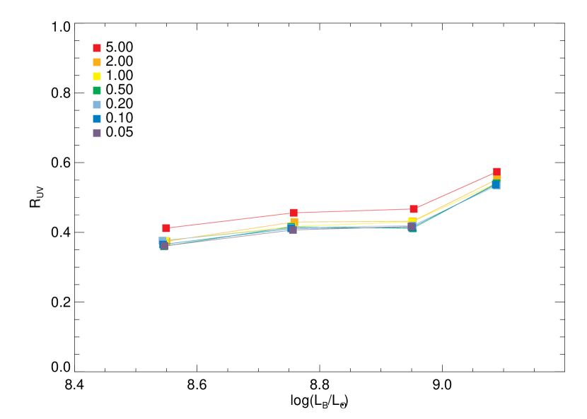
Figure 16: The effect of changing just the amount of titanium in the outer ejecta. Upper – UV colours; Middle – The positions of $\lambda_{1}$ and $\lambda_{2}$; Lower: $R_{UV}$

References

- Altavilla et al. (2004) Altavilla G., Fiorentino G., Marconi M., et al., 2004, MNRAS, 349, 1344
- Astier et al. (2006) Astier P., Guy J., Regnault N., et al., 2006, A&A, 447, 31
- Brown et al. (2010) Brown P. J., Roming P. W. A., Milne P., et al., 2010, ApJ, 721, 1608
- Bufano et al. (2009) Bufano F., Immler S., Turatto M., et al., 2009, ApJ, 700, 1456
- Conley et al. (2006) Conley A., Howell D. A., Howes A., et al., 2006, AJ, 132, 1707
- Conley et al. (2008) Conley A., Sullivan M., Hsiao E. Y., et al., 2008, ApJ, 681, 482
- Cooke et al. (2011) Cooke J., Ellis R. S., Sullivan M., et al., 2011, ApJ, 727, L35
- Ellis et al. (2008) Ellis R. S., Sullivan M., Nugent P. E., et al., 2008, ApJ, 674, 51
- Foley et al. (2008) Foley R. J., Filippenko A. V., Jha S. W., 2008, ApJ, 686, 117
- Foley et al. (2012) Foley R. J., Filippenko A. V., Kessler R., et al., 2012, AJ, 143, 113
- Garavini et al. (2007) Garavini G., Nobili S., Taubenberger S., et al., 2007, A&A, 471, 527
- Guy et al. (2007) Guy J., Astier P., Baumont S., et al., 2007, A&A, 466, 11
- Hamuy et al. (2000) Hamuy M., Trager S. C., Pinto P. A., et al., 2000, AJ, 120, 1479
- Höflich et al. (1998) Höflich P., Wheeler J. C., Thielemann F. K., 1998, ApJ, 495, 617
- Howell et al. (2009) Howell D. A., Sullivan M., Brown E. F., et al., 2009, ApJ, 691, 661
- Howell et al. (2007) Howell D. A., Sullivan M., Conley A., et al., 2007, ApJ, 667, L37
- Iwamoto et al. (1999) Iwamoto K., Brachwitz F., Nomoto K., et al., 1999, ApJ SS, 125, 439
- Kessler et al. (2009) Kessler R., Becker A. C., Cinabro D., et al., 2009, ApJ SS, 185, 32
- Lentz et al. (2000) Lentz E. J., Baron E., Branch D., et al., 2000, ApJ, 530, 966
- Lucy (1999) Lucy L. B., 1999, A&A, 345, 211
- Mazzali (2000) Mazzali P. A., 2000, A&A, 363, 705
- Mazzali & Lucy (1993) Mazzali P. A., Lucy L. B., 1993, A&A, 279, 447
- Mazzali & Podsiadlowski (2006) Mazzali P. A., Podsiadlowski P., 2006, MNRAS, 369, L19
- Milne et al. (2010) Milne P. A., Brown P. J., Roming P. W. A., et al., 2010, ApJ, 721, 1627
- Nomoto et al. (1984) Nomoto K., Thielemann F.-K., Yokoi K., 1984, ApJ, 286, 644
- Oke et al. (1995) Oke J. B., Cohen J. G., Carr M., et al., 1995, PASP, 107, 375
- Pastorello et al. (2007) Pastorello A., Taubenberger S., Elias-Rosa N., et al., 2007, MNRAS, 376, 1301
- Pauldrach et al. (1996) Pauldrach A. W. A., Duschinger M., Mazzali P. A., et al., 1996, A&A, 312, 525
- Perlmutter et al. (1999) Perlmutter S., Aldering G., Goldhaber G., et al., 1999, ApJ, 517, 565
- Perrett et al. (2010) Perrett K., Balam D., Sullivan M., et al., 2010, AJ, 140, 518
- Phillips (1993) Phillips M. M., 1993, ApJ, 413, L105
- Riess et al. (1998) Riess A. G., Filippenko A. V., Challis P., et al., 1998, AJ, 116, 1009
- Riess et al. (2007) Riess A. G., Strolger L.-G., Casertano S., et al., 2007, ApJ, 659, 98
- Sauer et al. (2006) Sauer D. N., Hoffmann T. L., Pauldrach A. W. A., 2006, A&A, 459, 229
- Sauer et al. (2008) Sauer D. N., Mazzali P. A., Blondin S., et al., 2008, MNRAS, 391, 1605
- Stehle et al. (2005) Stehle M., Mazzali P. A., Benetti S., et al., 2005, MNRAS, 360, 1231
- Sullivan et al. (2010) Sullivan M., Conley A., Howell D. A., et al., 2010, MNRAS, 406, 782
- Sullivan et al. (2011) Sullivan M., Guy J., Conley A., et al., 2011, ApJ, 737, 102
- Timmes et al. (2003) Timmes F. X., Brown E. F., Truran J. W., 2003, ApJ, 590, L83
- Walker et al. (2011) Walker E. S., Hook I. M., Sullivan M., et al., 2011, MNRAS, 410, 1262
- Wang et al. (2009) Wang X., Li W., Filippenko A. V., et al., 2009, ApJ, 697, 380
- Wang et al. (2012) Wang X., Wang L., Filippenko A. V., et al., 2012, ApJ, 749, 126
- Wood-Vasey et al. (2007) Wood-Vasey W. M., Miknaitis G., Stubbs C. W., et al., 2007, ApJ, 666, 694