Strain-induced metal-insulator phase coexistence and stability in perovskite manganites

Abstract

We present a detailed study of a model for strain-induced metal-insulator phase coexistence in perovskite manganites. Both nanoscale and mesoscale inhomogeneities are self-consistently described using atomic scale modes and their associated constraint equations. We also examine the stability of domain configurations against uniform and nonuniform modifications of domain walls. Our results show that the long range interactions between strain fields and the complex energy landscape with multiple metastable states play essential roles in stabilizing metal-insulator phase coexistence, as observed in perovskite manganites. We elaborate on the modes, constraint equations, energies, and energy gradients that form the basis of our simulation results.

I Introduction

Over the last several years, much attention has focused on the multiscale inhomogeneities observed in perovskite manganites. Salamon01 Unlike inhomogeneities for some other complex electronic systems, such as stripes in high-T_c cuprates, the coexistence of metallic and insulating phases within the same crystals of manganites has been directly observed through various high resolution local probes, such as dark field images and scanning microscopy. Uehara99 ; Fath99 ; Renner02 Nanoscale inhomogeneities have also been implied based on x-ray diffraction results. Kiryukhin04 Theories based on chemical randomness and electronic phase separation have been proposed as a mechanism for such inhomogeneities. Moreo99 ; Burgy04 However, theories based on chemical randomness alone assume an exact degeneracy between metallic and insulating phases, Burgy04 which ultimately leads to a homogeneous phase. Ahn04arxiv Also, the effect of the Coulomb interaction has not been incorporated adequately into the model describing electronic phase separation. Moreo99

We have previously proposed an intrinsic mechanism for phase coexistence, Ahn04 in which the interaction between strain fields plays an important role, as speculated in earlier literature. Mathur01 ; Millis03 ; Bishop03 Specifically, our model Ahn04 includes intrinsic complexity of the energy landscape and long range anisotropic interaction between strain fields, and shows how such physics can give rise to multiscale inhomogeneities observed in manganites. Our theoretical idea is supported by experimental results. Mathur04 For example, the observed large scale inhomogeneity of the order of 10 $\mu$m without any observable chemical inhomogeneity at a length scale of 0.5 $\mu$m or larger, suggests an intrinsic mechanism for the phase coexistence. Sarma04 The lamellar morphology of coexisting phases observed in manganites and the change of domain configurations upon thermal cycling between 10 K and 300 K further support this point of view. Tao05 It is also found that the anisotropic epitaxial strain in thin films gives rise to anisotropic percolation, which suggests that the origin of phase coexistence is much more strongly affected by long range strain rather than by local chemical inhomogeneity due to doping. Ward09

In contrast to the point of view in Refs. Moreo99, and Burgy04, that considers extrinsic mechanism such as chemical inhomogeneity and disorder as being key to understanding coexistence of metallic and insulating phases, our work proposes that the intrinsic mechanism, that is, the competition between the short and long range interactions, creates a delicate energy landscape that leads to domain formation. Further, the domain walls can be pinned by the atomistic Peierls-Nabarro force, rather than by disorder which is frequently attributed as being the cause for the phenomenon. Moreo99 ; Burgy04 We proposed the basic ideas in Ref. Ahn04, , but now develop them further and describe more extensive implementation of the approach here. Specifically, we present details of our model, methods, and results, as well as further simulations on the stability of phase coexistence. In Sect. II, the details of the Hamiltonian used for the simulations in Ref. Ahn04, , and results obtained with various initial conditions and parameters, are presented. We also contrast these results with simulations for a system that include short range interactions only. In Sect. III, we discuss the mechanism underlying the stability of micron-scale phase coexistence through further simulations and analysis. In Sect. IV, we summarize our main results. Expressions for energies and energy gradients used for simulations of the inhomogeneous states are provided in Appendices A and B, respectively.

II Model for strain-induced metal-insulator phase coexistence

II.1 Properties of manganites and requirements for phase coexistence in manganites

Perovskite manganites typically have the chemical formula $RE_{1-x}AK_{x}$MnO₃, where $RE$ represents rare earth elements, such as La, Nd, and Pr, and $AK$ represents alkali metal elements such as Ca and Sr. Millis98 ; Salamon01 ; Mathur03 The important electrons for both electronic properties and structures are the $e_{g}$ electrons on Mn ions: the degeneracy of the $e_{g}$ orbitals leads to a strong Jahn-Teller electron-lattice coupling. Shortly after the discovery of colossal magnetoresistance in these materials, Jin94 the importance of strong electron-lattice coupling was pointed out to explain the large resistivity above the ferromagnetic transition temperature in terms of dynamic Jahn-Teller polarons. Millis98 The same strong electron-lattice coupling is also responsible for a large structural difference between the low temperature metallic and insulating phases of these materials. In the insulating phase, the $e_{g}$ electrons are localized and the charge density forms an ordered pattern. The orbital states of the $e_{g}$ electrons, which are linear combinations of two $e_{g}$ orbital states, $x^{2}-y^{2}$ and $3z^{2}-r^{2}$, are also ordered. Due to the static Jahn-Teller effect, such a charge and orbital ordered state accompanies uniform and short wavelength lattice distortions. For example, the long Mn-O bond (or the elongated $e_{g}$ electron orbital) in La_0.5Ca_0.5MnO₃ alternates its direction in a plane, which gives rise to short wavelength lattice distortions. Chen96 Along the direction perpendicular to this plane, the short Mn-O bond repeats itself, and therefore the unit cell is compressed along this orientation, giving uniform or long-wavelength lattice distortions. In contrast, the lattice in the metallic ground state of manganites has a structure close to an ideal cubic perovskite structure without Jahn-Teller lattice distortions because the electrons are delocalized. The ground state can be changed between metallic and insulating phases in various ways, such as by the size of $RE$ and $AK$, applied magnetic fields, or applied pressures. Hwang95 ; Tokura96 ; Hwang95b

We propose that the first key to the understanding of the phase coexistence in manganites is the metastability, which has been observed in many experiments. For example, the distorted insulating phase of manganites can be transformed into the undistorted metallic phase by either x-rays Kiryukhin97 or magnetic fields, Tokura96 and the metallic phase does not revert to the insulating phase even after the external perturbation is removed. In particular, in x-ray experiments, Kiryukhin97 the reduction of the superlattice peak intensity and the simultaneous increase of conductivity, while the sample is exposed to the x-rays, demonstrate the transformation of the insulating phase into the metallic phase and the presence of inhomogeneity. However, an energy landscape with local and global energy minima is not sufficient to explain the observed sub-micron scale inhomogeneity, because such inhomogeneity is unstable against thermal fluctuations. As pointed out in Ref. Mathur03, , an unusual aspect of inhomogeneity in manganites is its stability over a 100 K range in temperature, which is an indication of an extra mechanism at play that affects phase coexistence in manganites.

Based on the strong electron-lattice coupling mentioned above and experiments showing the important role of strain in metal-insulator transition in manganites, Podzorov01 we propose that the extra mechanism should be related to the long range anisotropic interaction between strain fields. It is thus essential to consider the energy landscape in terms of the lattice distortion variables, which will ultimately have a bearing on other degrees of freedom such as magnetic moment or electron density. The origin of the long range anisotropic interaction within this framework is the bonding constraint, often referred to as strain compatibility. The compatibility condition enforces single-valued strain fields without broken bonds. Shenoy99 ; Lookman03 ; Ahn03 The anisotropy reflects the discrete rotational symmetry associated with the lattice structures. Such long-range anisotropic interactions are responsible, for example, for well-defined structural twin boundaries Ren02 over distances of 100 $\mu m$.

The cubic phase of perovskite manganites contains five atoms per unit cell. The insulating charge and orbital ordered phase consists of a zig-zag pattern of the long Mn-O bond orientation, which further increases the number of atoms per unit cell. Inclusion of such details is necessary for a complete description of properties of these materials. For the current study, however, we wish to focus on the following three key features of manganites essential for multiscale inhomogeneity, and capture them in a simple model. First, the metallic phase has almost no lattice distortions in comparison with the charge and orbital ordered insulating phase. Second, the insulating ground state has a uniform or long wavelength ($\vec{k}\sim 0$) lattice distortion. This property is essential because it is the long wavelength distortion, not the short wavelength one, that gives rise to the long range anisotropic interaction between strain fields. Third, the insulating phase has a short wavelength lattice distortion, in addition to the uniform distortion. As we will show below, the symmetry-allowed coupling between uniform and short-wavelength distortions gives rise naturally to an energy landscape with multiple minima.

II.2 Model system, variables and constraint equations

Before we introduce our model, we examine whether a simpler 2-dimensional (2D) model can be used instead of a 3-dimensional (3D) model, in particular to capture the effect of the long-range strain-strain interactions. In D-dimensional space (D = 2 or 3), the anisotropic strain-strain interaction decays as $1/r^{D}$, where $r$ represents the distance between two points. Shenoy99 ; Rasmussen01 ; Lookman03 The spatial integration of $1/r^{D}$ would give rise to a logarithmic divergence in both 2 and 3 dimensional space, Anisotropy which indicates that the effect of the interaction would be similar for both cases. Indeed, recent simulations of strains in 2 and 3 dimensional space show very similar results. Rasmussen01 ; Lookman03 Thus, we limit ourselves in this work to a 2D model for simplicity.

One of the simplest lattices in 2D space is the square lattice with a monatomic basis shown in Fig. 1. By considering one isotropic electron orbital per site and nearest neighbor electron hopping, the lattice supports a metallic electron density of states (DOS) without a gap. Therefore, such an undistorted square lattice shares the first property for manganites mentioned above. To include the second property, we deform the square unit cell of the lattice to a rectangular unit cell, either along the horizontal or vertical directions. To include the third property, we incorporate the $(\pi,\pi)$ type displacements of atoms along the horizontal (vertical) direction for a rectangular lattice elongated along the vertical (horizontal) direction. Rectangular lattices with such short wavelength lattice distortions support an electron DOS with a gap at the center, if we consider the natural electron hopping amplitude modulation by the changes in interatomic distances. Therefore, such lattices have an insulating DOS for the electron density of half an electron per site. Even though the 2D lattice described above is simple, it shares all the three properties of manganites that we believe are essential for the observed inhomogeneity, and provides a testing ground for whether the complex energy landscape and long range strain-strain interaction can indeed give rise to self-consistent multiscale inhomogeneities.

We require an energy expression for which the undistorted and distorted lattices described above are the local and global energy minimum states. For this purpose, we use an atomic-scale mode-based description of lattice distortions that we developed recently. Ahn03 In this method, we use normal modes of a square plaquette of four atoms, instead of displacement variables, to describe lattice distortions. These atomic scale modes for the monatomic square lattice are shown in Fig. 2. The first three modes are long wave length modes, since they can be obtained by uniformly deforming the square lattice. The last two modes, which correspond to $(\pi,\pi)$ staggered distortions of the lattice, are short wavelength modes. For a square lattice, each atom is shared by four neighboring plaquettes, which makes the modes at neighboring plaquettes dependent on each other. Such a constraint can be expressed in terms of equations in the Fourier transformed space, and the five modes can describe any lattice distortion for the square lattice with a monatomic basis. In the long wavelength limit, the three long wavelength modes become identical to the familiar strain modes, which makes our approach ideal for describing nano-and micro-meter scale inhomogeneities within the same theoretical framework. The inclusion of constraints allows our method to automatically generate the effects of the long range anisotropic interaction, the origin of which is the short-range bonding constraint.

We consider an $N\times N$ square lattice with a modified periodic condition explained below. The displacement variables for the atom at the site $\vec{i}$ are $u^{x}_{\vec{i}}$ and $u^{y}_{\vec{i}}$. The distance between the nearest neighbor atoms, $a$, is irrelevant to our formalism presented below, and can be chosen depending on the relative size of the distortions compared to the lattice constants. In all the figures in this paper, $a$ is chosen as 10 so that the size of the distortion relative to the interatomic distance is of the same order of the magnitude as observed in charge and orbital ordered manganites. In general, the displacement of atoms in a periodic structure can be described using two components. One is the component that changes monotonically as the site indices shift along a direction. This component, represented by a superscript ‘$nF$’ below, can not be Fourier-transformed and corresponds to the uniform distortion of the lattice. The rest of the displacement, represented by a superscript ‘$F$’ below, can be Fourier-transformed and is subject to the periodic boundary condition. Therefore, we express the displacements as follows:

$$u^{x}_{\vec{i}} = u^{x,nF}_{\vec{i}}+u^{x,F}_{\vec{i}},$$ (1)

$$u^{y}_{\vec{i}} = u^{y,nF}_{\vec{i}}+u^{y,F}_{\vec{i}},$$ (2)

where

$$u^{x,nF}_{\vec{i}} = \varepsilon^{xx}_{0}i_{x}+\varepsilon^{xy}_{0}i_{y},$$ (3)

$$u^{y,nF}_{\vec{i}} = \varepsilon^{xy}_{0}i_{x}+\varepsilon^{yy}_{0}i_{y},$$ (4)

and

$$u^{x,F}_{\vec{i}} = \sum_{\vec{k}}u^{x}_{\vec{k}}e^{i\vec{k}\cdot\vec{i}},$$ (5)

$$u^{y,F}_{\vec{i}} = \sum_{\vec{k}}u^{y}_{\vec{k}}e^{i\vec{k}\cdot\vec{i}}.$$ (6)

We note that $u^{x}_{\vec{k}}$ and $u^{y}_{\vec{k}}$ are obtained through the Fourier transformation of $u^{x,F}_{\vec{i}}$ and $u^{y,F}_{\vec{i}}$, rather than $u^{x}_{\vec{i}}$ and $u^{y}_{\vec{i}}$. The periodic boundary condition results in

$$k_{x} = \frac{2\pi n_{x}}{N},$$ (7)

$$k_{y} = \frac{2\pi n_{y}}{N},$$ (8)

where $n_{x}=-N/2-1,...,N/2$ and $n_{y}=-N/2-1,...,N/2$. For $u^{x,nF}_{\vec{i}}$ and $u^{y,nF}_{\vec{i}}$, the rigid rotation of the whole system is excluded, since it is irrelevant to the potential energy change. Similarly, the $\vec{k}=0$ components of $u^{x,F}_{\vec{i}}$ and $u^{y,F}_{\vec{i}}$ correspond to the rigid translation of the whole system, which are set to zero.

For the square lattice, we define the symmetry modes shown in Fig. 2 as follows:

$$e_{1}(\vec{i}) = \frac{1}{2\sqrt{2}}\left(-u^{x}_{\vec{i}}-u^{y}_{\vec{i}}+u^{x}_{\vec{i}+10}-u^{y}_{\vec{i}+10}-u^{x}_{\vec{i}+01}+u^{y}_{\vec{i}+01}+u^{x}_{\vec{i}+11}+u^{y}_{\vec{i}+11}\right),$$ (9)

$$e_{2}(\vec{i}) = \frac{1}{2\sqrt{2}}\left(-u^{x}_{\vec{i}}-u^{y}_{\vec{i}}-u^{x}_{\vec{i}+10}+u^{y}_{\vec{i}+10}+u^{x}_{\vec{i}+01}-u^{y}_{\vec{i}+01}+u^{x}_{\vec{i}+11}+u^{y}_{\vec{i}+11}\right),$$ (10)

$$e_{3}(\vec{i}) = \frac{1}{2\sqrt{2}}\left(-u^{x}_{\vec{i}}+u^{y}_{\vec{i}}+u^{x}_{\vec{i}+10}+u^{y}_{\vec{i}+10}-u^{x}_{\vec{i}+01}-u^{y}_{\vec{i}+01}+u^{x}_{\vec{i}+11}-u^{y}_{\vec{i}+11}\right),$$ (11)

$$s_{x}(\vec{i}) = \frac{1}{2}\left(u^{x}_{\vec{i}}-u^{x}_{\vec{i}+10}-u^{x}_{\vec{i}+01}+u^{x}_{\vec{i}+11}\right),$$ (12)

$$s_{y}(\vec{i}) = \frac{1}{2}\left(u^{y}_{\vec{i}}-u^{y}_{\vec{i}+10}-u^{y}_{\vec{i}+01}+u^{y}_{\vec{i}+11}\right).$$ (13)

These modes are fully subject to the periodic boundary condition, e.g., $e_{1}(i_{x},i_{y})=e_{1}(i_{x}+N,i_{y})=e_{1}(i_{x},i_{y}+N)$, unlike the displacement variables. Thus, they can be Fourier-transformed, for example, according to

$$e_{1}(\vec{i})=\sum_{\vec{k}}e_{1}(\vec{k})e^{i\vec{k}\cdot\vec{i}}.$$ (14)

From the definitions, we find

$$e_{1}(\vec{k}=0) = \frac{\varepsilon^{xx}_{0}+\varepsilon^{yy}_{0}}{\sqrt{2}}\equiv\tilde{e}_{1},$$ (15)

$$e_{2}(\vec{k}=0) = \frac{\varepsilon^{xy}_{0}}{\sqrt{2}}\equiv\tilde{e}_{2},$$ (16)

$$e_{3}(\vec{k}=0) = \frac{\varepsilon^{xx}_{0}-\varepsilon^{yy}_{0}}{\sqrt{2}}\equiv\tilde{e}_{3},$$ (17)

$$s_{x}(\vec{k}=0) = 0,$$ (18)

$$s_{y}(\vec{k}=0) = 0,$$ (19)

and

$$e_{1}(\vec{k}\neq 0) = \frac{1}{2\sqrt{2}}\left[-(1-e^{ik_{x}})(1+e^{ik_{y}})u^{x}_{\vec{k}}-(1+e^{ik_{x}})(1-e^{ik_{y}})u^{y}_{\vec{k}}\right],$$ (20)

$$e_{2}(\vec{k}\neq 0) = \frac{1}{2\sqrt{2}}\left[-(1+e^{ik_{x}})(1-e^{ik_{y}})u^{x}_{\vec{k}}-(1-e^{ik_{x}})(1+e^{ik_{y}})u^{y}_{\vec{k}}\right],$$ (21)

$$e_{3}(\vec{k}\neq 0) = \frac{1}{2\sqrt{2}}\left[-(1-e^{ik_{x}})(1+e^{ik_{y}})u^{x}_{\vec{k}}+(1+e^{ik_{x}})(1-e^{ik_{y}})u^{y}_{\vec{k}}\right],$$ (22)

$$s_{x}(\vec{k}\neq 0) = \frac{1}{2}(1-e^{ik_{x}})(1-e^{ik_{y}})u^{x}_{\vec{k}},$$ (23)

$$s_{y}(\vec{k}\neq 0) = \frac{1}{2}(1-e^{ik_{x}})(1-e^{ik_{y}})u^{y}_{\vec{k}}.$$ (24)

We note that the $\vec{k}=0$ components of the symmetry modes are from $u^{x,nF}_{\vec{i}}$ and $u^{y,nF}_{\vec{i}}$, while $\vec{k}=0$ components of $u^{x,F}_{\vec{i}}$ and $u^{y,F}_{\vec{i}}$ do not contribute to the distortion modes.

The five variables are related by three constraint equations, because only two physically independent displacement variables exist for each site. As discussed in Ref. Ahn03, , these constraint equations are found from the relations between the symmetry modes and the displacement variables in reciprocal space. For $k_{x}\neq 0$ and $k_{y}\neq 0$, we invert the linear relations between [$s_{x}(\vec{k})$, $s_{y}(\vec{k})$] and [$u^{x}_{\vec{k}}$, $u^{y}_{\vec{k}}$] in Eqs. (23) and (24) and replace them in the expressions with other modes in Eqs. (20)-(22). This leads to

$$\sin{\frac{k_{x}}{2}}\cos{\frac{k_{y}}{2}}s_{x}(\vec{k})+\cos{\frac{k_{x}}{2}}\sin{\frac{k_{y}}{2}}s_{y}(\vec{k})-\sqrt{2}i\sin{\frac{k_{x}}{2}}\sin{\frac{k_{y}}{2}}e_{1}(\vec{k}) = 0,$$ (25)

$$\cos{\frac{k_{x}}{2}}\sin{\frac{k_{y}}{2}}s_{x}(\vec{k})+\sin{\frac{k_{x}}{2}}\cos{\frac{k_{y}}{2}}s_{y}(\vec{k})-\sqrt{2}i\sin{\frac{k_{x}}{2}}\sin{\frac{k_{y}}{2}}e_{2}(\vec{k}) = 0,$$ (26)

$$\sin{\frac{k_{x}}{2}}\cos{\frac{k_{y}}{2}}s_{x}(\vec{k})-\cos{\frac{k_{x}}{2}}\sin{\frac{k_{y}}{2}}s_{y}(\vec{k})-\sqrt{2}i\sin{\frac{k_{x}}{2}}\sin{\frac{k_{y}}{2}}e_{3}(\vec{k}) = 0.$$ (27)

These constraint equations indicate that $e_{1}(\pi,\pi)$, $e_{2}(\pi,\pi)$, and $e_{3}(\pi,\pi)$ vanish and $\tilde{s}_{x}\equiv s_{x}(\pi,\pi)$ and $\tilde{s}_{y}\equiv s_{y}(\pi,\pi)$ are independent variables. Constraint equations for $k_{x}=0$ or $k_{y}=0$ should be considered separately from Eqs. (25)-(27). Equations (15)-(19) show that $e_{1}(\vec{k}=0)$, $e_{2}(\vec{k}=0)$ and $e_{3}(\vec{k}=0)$ are independent of each other, and $s_{x}(\vec{k}=0)$ and $s_{y}(\vec{k}=0)$ vanish. For $k_{x}=0$ and $k_{y}\neq 0$, Eqs. (20)-(24) show that $e_{1}(\vec{k})=-e_{3}(\vec{k})$ and $e_{2}(\vec{k})$ are independent variables, and $s_{x}(\vec{k})=s_{y}(\vec{k})=0$. Similarly, for $k_{x}\neq 0$ and $k_{y}=0$, $e_{1}(\vec{k})=e_{3}(\vec{k})$ and $e_{2}(\vec{k})$ are independent variables, and $s_{x}(\vec{k})=s_{y}(\vec{k})=0$.

To describe lattice distortions in our simulations, we primarily use the variables $s_{x}(\vec{i})$ and $s_{y}(\vec{i})$. These variables can be assigned arbitrarily except that they should satisfy $s_{x}(\vec{k})=s_{y}(\vec{k})=0$ if $k_{x}=0$ or $k_{y}=0$, as required by Eqs. (18), (19), (23), and (24). In our numerical simulations, we implement this condition by subtracting unphysical components with $k_{x}=0$ or $k_{y}=0$ from $s_{x}(\vec{i})$ and $s_{y}(\vec{i})$, each time we initialize or change $s_{x}(\vec{i})$ and $s_{y}(\vec{i})$. However, $s_{x}(\vec{i})$ and $s_{y}(\vec{i})$ do not uniquely determine lattice distortions, because of the singular relation between [$s_{x}(\vec{k})$, $s_{y}(\vec{k})$] and [$u^{x}_{\vec{k}}$, $u^{y}_{\vec{k}}$] in Eqs. (23) and (24). As seen above, $e_{1}(\vec{k}=0)$, $e_{2}(\vec{k}=0)$, $e_{3}(\vec{k}=0)$, $e_{1}(k_{x}=0,k_{y}\neq 0)=-e_{3}(k_{x}=0,k_{y}\neq 0)$, $e_{2}(k_{x}=0,k_{y}\neq 0)$, $e_{1}(k_{x}\neq 0,k_{y}=0)=e_{3}(k_{x}\neq 0,k_{y}=0)$, and $e_{2}(k_{x}\neq 0,k_{y}=0)$ should be specified, in addition to $s_{x}(\vec{i})$ and $s_{y}(\vec{i})$, for the complete description of lattice distortions.

From these variables, displacement variables, $u^{x}_{\vec{i}}$ and $u^{y}_{\vec{i}}$, are calculated. For the non-periodic parts of displacements, $u_{\vec{i}}^{x,nF}$ and $u_{\vec{i}}^{y,nF}$ in Eqs. (3) and (4), we use Eqs. (15)-(17) to obtain

$$u_{\vec{i}}^{x,nF} = \frac{e_{1}(\vec{k}=0)+e_{3}(\vec{k}=0)}{\sqrt{2}}i_{x}+\sqrt{2}e_{2}(\vec{k}=0)i_{y},$$ (28)

$$u_{\vec{i}}^{y,nF} = \sqrt{2}e_{2}(\vec{k}=0)i_{x}+\frac{e_{1}(\vec{k}=0)-e_{3}(\vec{k}=0)}{\sqrt{2}}i_{y}.$$ (29)

We find the periodic parts of the displacement, $u_{\vec{i}}^{x,F}$ and $u_{\vec{i}}^{y,F}$, through the Fourier transformation of $u^{x}_{\vec{k}}$ and $u^{y}_{\vec{k}}$, which are obtained by inverting two non-singular equations among Eqs. (20)-(24). Therefore, if $k_{x}\neq 0$ and $k_{y}\neq 0$, we invert Eqs. (23) and (24) to obtain

$$u^{x}_{k_{x}\neq 0,k_{y}\neq 0}=\frac{2}{(1-e^{ik_{x}})(1-e^{ik_{y}})}s_{x}(\vec{k}),$$ (30)

$$u^{y}_{k_{x}\neq 0,k_{y}\neq 0}=\frac{2}{(1-e^{ik_{x}})(1-e^{ik_{y}})}s_{y}(\vec{k}).$$ (31)

If $k_{x}\neq 0$ and $k_{y}=0$, Eqs. (20) and (21) lead to

$$u^{x}_{k_{x}\neq 0,k_{y}=0}=-\frac{\sqrt{2}}{1-e^{ik_{x}}}e_{1}(\vec{k}),$$ (32)

$$u^{y}_{k_{x}\neq 0,k_{y}=0}=-\frac{\sqrt{2}}{1-e^{ik_{x}}}e_{2}(\vec{k}).$$ (33)

Similarly, if $k_{x}=0$ and $k_{y}\neq 0$, we obtain

$$u^{x}_{k_{x}=0,k_{y}\neq 0}=\frac{\sqrt{2}}{1-e^{ik_{y}}}e_{2}(\vec{k}),$$ (34)

$$u^{y}_{k_{x}=0,k_{y}\neq 0}=\frac{\sqrt{2}}{1-e^{ik_{y}}}e_{1}(\vec{k}).$$ (35)

The $k_{x}=0$ and $k_{y}=0$ components of the displacements correspond to rigid displacements, which are set to zero:

$$u^{x}_{k_{x}=0,k_{y}=0}=0,$$ (36)

$$u^{y}_{k_{x}=0,k_{y}=0}=0.$$ (37)

By adding periodic and non-periodic parts of displacements according to Eqs. (1) and (2), we find $u^{x}_{\vec{i}}$ and $u^{y}_{\vec{i}}$.

II.3 Total energy of the model and the Hamiltonian for electronic property calculations

In terms of the above modes, we consider the following energy expression, $E_{tot}$, as the total energy of a model system for strain-induced phase coexistence: Ahn04

$$E_{tot}=E_{s}+E_{l}+E_{c},$$ (38)

$$E_{s}=\sum_{\vec{i}}\left[\frac{B}{2}(s_{x}^{2}+s_{y}^{2})+\frac{G_{1}}{4}(s_{x}^{4}+s_{y}^{4})+\frac{G_{2}}{2}s_{x}^{2}s_{y}^{2}+\frac{H_{1}}{6}(s_{x}^{6}+s_{y}^{6})+\frac{H_{2}}{6}s_{x}^{2}s_{y}^{2}(s_{x}^{2}+s_{y}^{2})\right]_{\vec{i}},$$ (39)

$$E_{l}=\sum_{\vec{i}}\left[\frac{A_{1}}{2}e_{1}^{2}+\frac{A_{2}}{2}e_{2}^{2}+\frac{A_{3}}{2}e_{3}^{2}\right]_{\vec{i}},$$ (40)

$$E_{c}=\sum_{\vec{i}}\left[C_{3}(s_{x}^{2}-s_{y}^{2})e_{3}\right]_{\vec{i}}.$$ (41)

The first term $E_{s}$ with short wavelength modes includes all symmetry-allowed terms up to sixth order with all coefficients positive, since we are interested in a first-order-transition-like energy landscape. The second term $E_{l}$ with long wavelength modes up to second order mediates the long range anisotropic interactions. The third term $E_{c}$ represents the coupling between the long and the short wavelength modes, where the $e_{3}$ mode is coupled to the $s_{x}$ and $s_{y}$ modes in a symmetry-allowed form. This last term gives rise to the global energy minimum state with long and short wavelength distortions, in addition to the local energy minimum state without distortion. The energy expression $E_{tot}$ gives rise to the desired energy landscape in appropriate ranges of parameters.

To establish a connection between the electronic properties and the lattice distortions as observed in manganites, namely metallic and insulating states for the undistorted and distorted phases, respectively, we use the following Su-Shrieffer-Heeger (SSH) Hamiltonian for the electronic structure calculations in our model:

$$H_{SSH} = \sum_{\vec{i}}-t_{0}\left[1-\alpha(u^{x}_{\vec{i}+(10)}-u^{x}_{\vec{i}})\right]\left(c^{\dagger}_{\vec{i}}c_{\vec{i}+(10)}+c^{\dagger}_{\vec{i}+(10)}c_{\vec{i}}\right)$$ (42)

$$-t_{0}\left[1-\alpha(u^{y}_{\vec{i}+(01)}-u^{y}_{\vec{i}})\right]\left(c^{\dagger}_{\vec{i}}c_{\vec{i}+(01)}+c^{\dagger}_{\vec{i}+(01)}c_{\vec{i}}\right).$$

Here, we consider only one orbital per site and neglect the electron spin for simplicity. The operator $c^{\dagger}_{\vec{i}}$ is the creation operator of an electron at a site $\vec{i}$. In this Hamiltonian, the electron hopping amplitude is assumed to be linearly modified by the change in the nearest neighbor interatomic distances. We make the adiabatic assumption that the total energy $E_{tot}$ is obtained by minimizing the energy of the system with respect to all degrees of freedom, including the electronic one, except for the lattice degrees of freedom. Therefore, $E_{tot}$ is used for the calculation of the energy landscape and the Euler simulations, whereas $H_{SSH}$ is used for the calculations of electronic properties associated with templates of lattice distortions.

The SSH Hamiltonian is a Hamiltonian for independent electrons, and can be diagonalized within a one-electron basis. Therefore, we construct electronic Hamiltonian matrices for given lattice distortions, $u^{x}_{\vec{i}}$ and $u^{y}_{\vec{i}}$, with the basis set $\{c^{\dagger}_{\vec{i}}|0\rangle\}$, where $|0\rangle$ represents the state without electrons. We diagonalize the matrices numerically, and fill the eigenstates with electrons according to the electron density. Representing the $l$-th lowest energy eigenstate as

$$|l\rangle=\sum_{\vec{i}}z_{l,\vec{i}}c^{\dagger}_{\vec{i}}|0\rangle,$$ (43)

the local DOS at site $\vec{i}$ is calculated by

$$D_{\vec{i}}(E)=\sum_{l}\delta(E-E_{l})|z_{l,\vec{i}}|^{2},$$ (44)

which reveals local electronic properties. The same approach has been used in Ref. Ahn05, to study electronic inhomogeneities around structural twin and antiphase boundaries in model systems with a strong electron-lattice coupling.

II.4 Energy landscape for homogeneous states

We expect the ground state of the model energy expression $E_{tot}$ to be homogeneous with $\tilde{e}_{1}$, $\tilde{e}_{2}$, $\tilde{e}_{3}$, $\tilde{s}_{x}$ and $\tilde{s}_{y}$ distortions only, defined in Eqs. (15)-(17) and below Eq. (27), considering the way that the energy terms are selected. Therefore, we study the following energy expression, which includes these particular distortions only, to understand the energy landscape for the homogeneous states:

$$E_{tot}^{h} = E_{s}^{h}+E_{l}^{h}+E_{c}^{h},$$ (45)

$$\frac{E_{s}^{h}}{N^{2}} = \frac{B}{2}\left(\tilde{s}_{x}^{2}+\tilde{s}_{y}^{2}\right)+\frac{G_{1}}{4}\left(\tilde{s}_{x}^{4}+\tilde{s}_{y}^{4}\right)+\frac{G_{2}}{2}\tilde{s}_{x}^{2}\tilde{s}_{y}^{2}+\frac{H_{1}}{6}\left(\tilde{s}_{x}^{6}+\tilde{s}_{y}^{6}\right)+\frac{H_{2}}{6}\tilde{s}_{x}^{2}\tilde{s}_{y}^{2}\left(\tilde{s}_{x}^{2}+\tilde{s}_{y}^{2}\right),$$ (46)

$$\frac{E_{l}^{h}}{N^{2}} = \frac{A_{1}}{2}\tilde{e}_{1}^{2}+\frac{A_{2}}{2}\tilde{e}_{2}^{2}+\frac{A_{3}}{2}\tilde{e}_{3}^{2},$$ (47)

$$\frac{E_{c}^{h}}{N^{2}} = C_{3}\left(\tilde{s}_{x}^{2}-\tilde{s}_{y}^{2}\right)\tilde{e}_{3}.$$ (48)

Because $\tilde{e}_{1}$, $\tilde{e}_{2}$, $\tilde{e}_{3}$, $\tilde{s}_{x}$ and $\tilde{s}_{y}$ are independent of each other, we minimize $E_{tot}^{h}$ with respect to $\tilde{e}_{1}$, $\tilde{e}_{2}$, and $\tilde{e}_{3}$ independently and obtain $\tilde{e}_{1}=0$, $\tilde{e}_{2}=0$, and $\tilde{e}_{3}=-C_{3}(\tilde{s}_{x}^{2}-\tilde{s}_{y}^{2})/A_{3}$. We insert these back into $E_{tot}^{h}$ and obtain the following energy expression in terms of $\tilde{s}_{x}$ and $\tilde{s}_{y}$ only:

$$\frac{E_{tot}^{h,min}}{N^{2}} = \frac{B}{2}\left(\tilde{s}_{x}^{2}+\tilde{s}_{y}^{2}\right)+\frac{1}{4}\left(G_{1}-2\frac{C_{3}^{2}}{A_{3}}\right)\left(\tilde{s}_{x}^{4}+\tilde{s}_{y}^{4}\right)+\frac{1}{2}\left(G_{2}+2\frac{C_{3}^{2}}{A_{3}}\right)\tilde{s}_{x}^{2}\tilde{s}_{y}^{2}$$ (49)

$$+\frac{H_{1}}{6}\left(\tilde{s}_{x}^{6}+\tilde{s}_{y}^{6}\right)+\frac{H_{2}}{6}\tilde{s}_{x}^{2}\tilde{s}_{y}^{2}\left(\tilde{s}_{x}^{2}+\tilde{s}_{y}^{2}\right).$$

We find parameter values, for which $E_{tot}^{h,min}/N^{2}$ has one local energy minimum state without distortion and four symmetry-related degenerate global energy minimum states with distortions. Necessary conditions for such first-order-transition-like energy landscape are $G_{1}^{\prime}\equiv G_{1}-2C_{3}^{2}/A_{3}<0$ and $(G_{1}^{\prime})^{2}>4BH_{1}$, for which the energy minima occur at $(\tilde{s}_{x},\tilde{s}_{y})=(0,0)$, $(\pm s_{0},0)$, and $(0,\pm s_{0})$ with

$$s_{0}=\sqrt{\frac{-G_{1}^{\prime}+\sqrt{(G_{1}^{\prime})^{2}-4BH_{1}}}{2H_{1}}}.$$ (50)

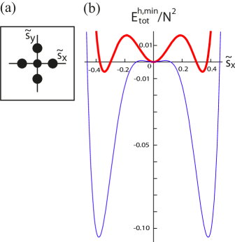
Figure 3: (Color online) Energy landscape for the homogeneous phase. (a) Solid dots mark the locations of local and global energy minima for $E^{h,min}_{tot}/N^{2}$ in Eq. (49) in the $\tilde{s}_{x}-\tilde{s}_{y}$ plane, where $\tilde{s}_{x}=s_{x}(\pi,\pi)$ and $\tilde{s}_{y}=s_{y}(\pi,\pi)$. The local energy minimum states with the opposite signs of $\tilde{s}_{x}$ or $\tilde{s}_{y}$ are related by a phase difference of the short wavelength distortion, whereas the local energy minimum states along $\tilde{s}_{x}$ axis is related to those along $\tilde{s}_{y}$ axis by the exchange of $x$ and $y$ axes. (b) $E^{h,min}_{tot}/N^{2}$ versus $\tilde{s}_{x}$ with $\tilde{s}_{y}=0$ for the two chosen parameter sets. The parameter values for the deep local energy minimum case, represented by the thick red curve, are $A_{1}=7$, $A_{2}=4$, $A_{3}=6$, $B=2$, $C_{3}=20$, $G_{1}=60$, $G_{2}=80$, $H_{1}=480$, and $H_{2}=640$, for which $G^{\prime}_{1}=-73.3$, $G^{\prime}_{2}\equiv G_{2}+2C_{3}^{2}/A_{3}=213$, $s_{0}=0.34$, and $|\tilde{e}_{3}|=0.39$, and $E_{tot}^{h,min}/N^{2}$ has a value of -0.0058 for the global energy minimum states. The height of the energy barrier between local and global energy minima is 0.0160, measured from the local energy minimum. The only different parameter value for the shallow local minimum case, represented by the thin blue curve, is $B=0.5$, which gives rise to $s_{0}=0.38$, $|\tilde{e}_{3}|=0.49$, the global energy minimum $E_{tot}^{h,min}/N^{2}$ of -0.1053, and energy barrier of 0.0009. Such difference in the energy landscape can be related, for example, to the average size of the rare earth and alkali metal elements in manganites.

The locations of the five energy minima in the $\tilde{s}_{x}-\tilde{s}_{y}$ plane are indicated in Fig. 3(a). Corresponding uniform mode distortions are $\tilde{e_{3}}=-C_{3}s_{0}^{2}/A_{3}$ for $(\tilde{s}_{x},\tilde{s}_{y})=(\pm s_{0},0)$, and $\tilde{e_{3}}=C_{3}s_{0}^{2}/A_{3}$ for $(\tilde{s}_{x},\tilde{s}_{y})=(0,\pm s_{0})$. For comparison, we choose two sets of parameter values, one giving a shallow and the other a deep local energy minimum at $(\tilde{s}_{x},\tilde{s}_{y})=(0,0)$, as shown with a thin blue and a thick red curve, respectively, in Fig. 3(b). In manganites, the difference in the depth of the energy landscape can be related to the size of rare earth or alkali metal elements, which is known experimentally to influence the physical properties of manganites. Hwang95 Alternatively, we may consider this a measure of “microstrain”. Bianconi

II.5 Methods of simulations for inhomogeneous states

The energy landscape is much more complicated for inhomogeneous states because of the constraint relations among the distortion modes. To study inhomogeneous configurations, particularly, metastable configurations, we first minimize $E_{tot}$ analytically with respect to all the independent variables except $s_{x}(\vec{i})$ and $s_{y}(\vec{i})$, that is, $e_{1}(\vec{k}=0)$, $e_{2}(\vec{k}=0)$, $e_{3}(\vec{k}=0)$, $e_{1}(k_{x}=0,k_{y}\neq 0)=-e_{3}(k_{x}=0,k_{y}\neq 0)$, $e_{2}(k_{x}=0,k_{y}\neq 0)$, $e_{1}(k_{x}\neq 0,k_{y}=0)=e_{3}(k_{x}\neq 0,k_{y}=0)$, and $e_{2}(k_{x}\neq 0,k_{y}=0)$, and obtain an energy expression $E^{\prime}_{tot}(s_{x},s_{y})$. The details of the derivation and expression for $E^{\prime}_{tot}(s_{x},s_{y})$ are provided in Appendix A.

In our simulations, we set initial configurations of $s_{x}(\vec{i})$ and $s_{y}(\vec{i})$ and relax the lattice according to the Euler method,

$$s_{x}^{n+1}(\vec{i}) = s_{x}^{n}(\vec{i})-\gamma\left.\frac{\partial E^{\prime}_{tot}(s_{x},s_{y})}{\partial s_{x}(\vec{i})}\right|_{s_{x}^{n},s_{y}^{n}},$$ (51)

$$s_{y}^{n+1}(\vec{i}) = s_{y}^{n}(\vec{i})-\gamma\left.\frac{\partial E^{\prime}_{tot}(s_{x},s_{y})}{\partial s_{y}(\vec{i})}\right|_{s_{x}^{n},s_{y}^{n}},$$ (52)

where the superscript $n$ or $n+1$ represents the number of Euler steps taken from the initial configuration, and $\gamma$ controls the size of the Euler step. Expressions for $\partial E^{\prime}_{tot}(s_{x},s_{y})/\partial s_{x}(\vec{i})$ and $\partial E^{\prime}_{tot}(s_{x},s_{y})/\partial s_{y}(\vec{i})$ are provided in Appendix B. We change $s_{x}(\vec{i})$ and $s_{y}(\vec{i})$ for all $\vec{i}$’s simultaneously at each step. We run the simulation until $E^{\prime}_{tot}(s_{x},s_{y})$ does not decrease further, but only fluctuates, which is an indication that the system has reached a local energy minimum configuration.

II.6 Initial conditions and results of the simulations for inhomogeneous states

We describe initial conditions, parameters, and results of the simulations in this subsection. Figure 4 shows the results of the simulations carried out on a $32\times 32$ lattice for the energy landscape with a shallow local minimum, shown in thin blue curve in Fig. 3(b) for homogeneous states. The color of each plaquette represents $p_{3}(\vec{i})\equiv s_{x}(\vec{i})^{2}-s_{y}(\vec{i})^{2}$, and the vertices and distortions of the plaquettes represent the actual locations of atoms and actual distortions. Through the coupling between $p_{3}$ and $e_{3}$ in $E_{c}$, positive and negative values of $p_{3}$ are usually accompanied by an $e_{3}$ distortion elongated along $y$ and $x$ direction, respectively. Most plaquettes with $p_{3}$ close to zero have little distortion. Starting from an initial configuration of $s_{x}(\vec{i})$ and $s_{y}(\vec{i})$, randomly chosen between $-2s_{0}$ and $2s_{0}$, as shown in Fig. 4(a), the system is relaxed through the Euler method with $\gamma=0.0015$. Figures 4(b)-4(h) correspond to the configurations at the Euler step $n=$100, 400, 1000, 2000, 4000, and 6000, and the stable configuration at $n=$100000, respectively. Final

Following the energy gradient from a random initial configuration, the simulation approximately represents a rapid quenching of the system from a very high temperature to 0 K. The result shows that most of the system initially changes into the undistorted state, as suggested in Fig. 4(d). Random fluctuations of $p_{3}$ tend to cancel each other when averaged over several interatomic distances, which prevents most regions from evolving into a global energy minimum state with lattice distortions. Some regions with relatively large distortions in the initial configuration evolve into a distorted state, as shown in Figs. 4(b)-4(d), and nucleate the distorted phase. These distorted regions expand into the undistorted region [Figs. 4(e)-4(g)], and eventually transforms most of the system into a distorted global energy minimum state separated by anti-phase boundaries, as shown in Fig. 4(h). We also find that there is a critical size for this nucleation: a distorted region of a small size in Fig. 4(c) changes into the undistorted state in Fig. 4(d). Such nucleation and growth observed in our simulations of the rapid quenching, and the presence of the critical size for the nucleation, reflect the first-order-transition-like energy landscape, and are features observed even in systems with only short range interactions.

For contrast, we study a system with a similar energy landscape, but without the long range interaction. For this we consider the following energy expression:

$$E_{M} = \sum_{\vec{i}}\frac{W}{2}M(\vec{i})^{2}+\frac{X}{4}M(\vec{i})^{2}+\frac{Y}{6}M(\vec{i})^{6}$$ (53)

$$+\frac{Z}{2}\left\{[M(\vec{i}+(1,0))-M(\vec{i})]^{2}+[M(\vec{i}+(0,1))-M(\vec{i})]^{2}\right\},$$

where $M(\vec{i})$ is defined at each site. The last term becomes $Z(\nabla M)^{2}/2$, the familiar Ginzburg-Landau gradient term, in the continuum limit. The gradient term of $E_{M}$ with respect to $M(\vec{i})$ for the Euler method is

$$\frac{\partial E_{M}}{\partial M(\vec{i})} = WM(\vec{i})+XM(\vec{i})^{3}+YM(\vec{i})^{5}$$ (54)

$$+ Z[4M(\vec{i})-M(\vec{i}-(1,0))-M(\vec{i}+(1,0))-M(\vec{i}-(0,1))-M(\vec{i}+(0,1))].$$

The parameters $W$, $X$, and $Y$ are chosen to be identical to the parameters $B$, $G^{\prime}_{1}$, and $H_{1}$ for the lattice model with a shallow local minimum in Fig. 3(b). We choose $Z=5$, similar to $A_{1}$, $A_{2}$ and $A_{3}$, since $e_{1}(\vec{i})$, $e_{2}(\vec{i})$, and $e_{3}(\vec{i})$ are related to the gradient of $s_{x}(\vec{i})$ and $s_{y}(\vec{i})$ in the continuum limit. Ahn03 The uniform ground state for $E_{M}$ is $M(\vec{i})=\pm M_{0}$, where

$$M_{0}=\sqrt{\frac{-X+\sqrt{X^{2}-4WY}}{2Y}}.$$ (55)

The selected parameter values result in $M_{0}=0.38$, identical to $s_{0}$ for the lattice distortion model. Figure 5 shows the results of the simulations on a $32\times 32$ lattice, in which $p=M^{2}$, analogous to $p_{3}$ for the lattice distortion model, is shown. The initial $M(\vec{i})$, shown in Fig. 5(a), is chosen randomly between $-5.3M_{0}$ and $5.3M_{0}$, and is relaxed according to the Euler method with $\gamma=0.00015$. The configurations at the Euler step $n=$ 1000, 4000, 10000, 2000, 40000, and 60000 are shown in Figs. 5(b)-5(g). The final stable configuration at $n=$ 1000000 is shown in Fig. 5(h). These Euler steps are chosen so that they are consistent with the Euler steps in Fig. 4 after being multiplied by $\gamma$. The system with a short range anisotropic interaction in Fig. 5 also shows nucleation and growth of the low energy phase. However, comparing Figs. 4 and  5 reveals distinct features present only in the lattice distortion model.

First, the nucleation droplets in Figs. 4(c)-4(e) are highly anisotropic, in contrast with those in Figs. 5(c)-5(e). Second, distortions separated by relatively large distance along the diagonal direction interact with each other, grow toward each other, and merge through the long range interaction, as seen for the yellow and red band along the 135 degree orientations in Figs. 4(c)-4(f). Third, the nucleation occurs via pairs of distortions with different orientations to minimize the interface energy between the distorted region and the undistorted background, as shown in Figs. 4(c) and 4(d). Such features are absent in Fig. 5, where the interaction is purely short-ranged. Recent x-ray scattering experiments have revealed the presence of short-range anisotropic precursor correlations in the orthorhombic phase of manganites at high temperatures, which disappear in the rhombohedral phase. Kiryukhin04 Such a feature has a similarity with the anisotropic droplets observed in our simulations, and is reminiscent of the precursor embryonic fluctuation in martensitic transformations. Seto90 The quasi-elastic central peak observed in manganites Lynn96 ; Lynn97 near the metal-insulator phase transition temperature is also likely to have a structural origin, similar to the central peak observed in ferroelectrics. Such experimental observations Kim00 and similar features seen in our simulations indicate that the strain plays an important role in the formation of nanometer scale inhomogeneity in manganites.

To demonstrate electronic inhomogeneity associated with the structural inhomogeneity, we calculate electronic properties for the template of the lattice distortions in Fig. 4(f). We use the SSH Hamiltonian in Eq. (42) with $t_{0}=1$ and $\alpha=1$. The typical local electron densities of states within undistorted and distorted regions are shown in Fig. 6(b). The local DOS is symmetric about $E=0$, and a gap (or a “pseudogap”) opens near $E=0$ in distorted regions. The small DOS within the gap for the distorted region is due to electron wavefunctions exponentially decaying from the undistorted region. Therefore, distorted and undistorted regions have insulating and metallic electron DOS at a half filling without any spatial charge inhomogeneity. The map of the local electron DOS at $E=0$ is shown in Fig. 6(a). The possible inhomogeneity in local DOS without any charge inhomogeneity in our model is in contrast with other explanations for the inhomogeneity based on electronic phase separation, an idea similar to the phase separation in binary alloys. Moreo99

Figure 7 shows results of a simulation with parameters identical to those in Fig. 4 except for a narrower range of the random initial values of $s_{x}(\vec{i})$ and $s_{y}(\vec{i})$ between $-s_{0}$ and $s_{0}$. Instead of multiple nucleations, only one nucleation emerges within the $32\times 32$ lattice, which grows and evolves the whole system into a periodic patten of stripes with positive and negative $p_{3}$. The final state shown in Fig. 7(f) is another metastable phase not considered in Fig. 3, where distortions only with a wave vector $(\pi,\pi)$ are considered. The result shows that multiple inequivalent metastable phases exist even in this simple model, and the coexistence of more than two phases is possible, as suggested in some manganites. Lee02 We use an even narrower range of the random initial $s_{x}(\vec{i})$ and $s_{y}(\vec{i})$ between $-s_{0}/2$ and $s_{0}/2$, in which case the system fails to nucleate a distorted region and remains in the undistorted phase, showing the characteristic metastability of systems with a first-order-transition energy landscape. The above results indicate that the low temperature metastable configurations depend sensitively on how the configurations are obtained, consistent with path-dependent experiments in manganites, such as the sensitivity to the cooling rate or strain glass behaviors. Wu06

For the deep local energy minimum case described by the thick red curve in Fig. 3(b), the simulation of rapid quenching using the Euler method for a $64\times 64$ lattice does not create nucleation of the low energy phase. Instead, we always obtain the undistorted homogeneous state as the final state, which is an indication of strong metastability due to a higher energy barrier between the distorted and the undistorted states. In crystals, we expect line or planar defects, as well as thermal fluctuations, would assist nucleation. Simulations of such processes require more computational resources. Therefore, we start from a predesigned initial condition and relax the lattice to obtain stable coexistence of distorted and undistorted domains. The initial condition is chosen on a $64\times 64$ lattice according to

$$s_{x}(i_{x},i_{y}) = s_{0}(-1)^{i_{x}+i_{y}}\left\{\cos\left[\frac{2\pi(i_{x}+i_{y}-4)}{N}\right]+0.5\right\},$$ (56)

$$s_{y}(i_{x},i_{y}) = 0,$$ (57)

where $N=64$. The initial configuration is relaxed with $\gamma=0.0002$, and the stable configuration is obtained, which is shown in Fig. 8(a). We find stable coexistence of large undistorted [green region in Fig. 8(a)] and distorted [red region in Fig. 8(a)] domains, unlike the shallow local minimum case studied above. The size of the domain is determined only by the initial condition, and therefore can be as large as several micrometers, consistent with experiments for manganites.

For comparison, we carry out simulations for a $N\times N$ system with a short range interaction only, described by $E_{M}$ in Eq. (53) with the parameter $W=2.0$, with a similar predesigned initial condition,

$$M(i_{x},i_{y})=M_{0}\left\{\cos\left[\frac{2\pi(i_{x}+i_{y})}{N}\right]+c_{s}\right\}.$$ (58)

For $c_{s}=0.5$, $\gamma=0.0002$, and $N=64$, we find that the final stable configuration is a uniform ground state for this system with a short interaction only, rather than a state with domains. For $c_{s}=0$, $\gamma=0.0002$, and $N=128$, we find only a line of atoms, rather than a domain, with $M$ close to zero between regions with $M=M_{0}$ and $M=-M_{0}$. This comparison shows that the strain-strain long range interaction indeed plays an essential role for the coexistence of distorted and undistorted phases.

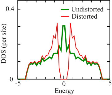
Figure 9: (Color online) Local electron DOS calculated at the center of an undistorted region (thick green line), $\vec{i}=(36,1)$ in Fig. 8(a), and at the center of a distorted region (thin red line), $\vec{i}=(6,1)$ in Fig. 8(a). Unlike the case of small domains in Fig. 6, a clear gap opens inside the large domain of distorted phase. The local density of states is always symmetric with respect to $E=0$. Therefore, for $E_{F}=0$, the electron number is 0.5 at all sites, demonstrating that the metal-insulator domain structure does not requires charge inhomogeneity.

For the configuration in Fig. 8(a), the local DOS versus energy is calculated at the centers of the undistorted region and the distorted region, which is shown in Fig. 9. The local DOS within the undistorted regions shows a metallic DOS without a gap, whereas the local DOS within the distorted region shows an insulating DOS with a gap around $E=0$. Therefore, for the chemical potential chosen at $E=0$ inside this gap, we obtain the coexistence of metallic undistorted and insulating distorted regions, as shown in Fig. 8(b), similar to experiment results. We also find that the interface between the metallic and insulating regions is rather sharp, consistent with STM images of atomically sharp interface between metallic and insulating domains in manganites. Renner02 Our results indicate that chemical inhomogeneity is not a necessary condition to have a large scale coexistence of metallic and insulating domains, which is in contrast to other theories. Burgy04 Although the lattice defects or segregation of dopants could play a role in nucleation, the stability of coexistence relies on the intrinsic energy landscape, which explains why external perturbations such as focused x-rays, Kiryukhin97 light, Fiebig98 or electron beams alter metallic and insulating domains.

III Stability of phase coexistence

III.1 Stability against uniform domain wall motions

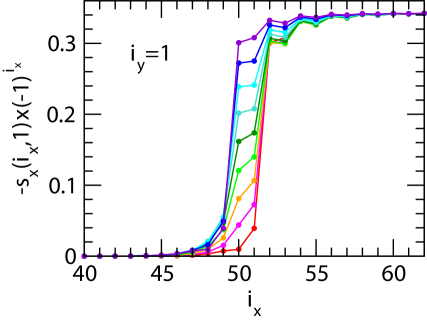
Figure 10: (Color online) The red dots represent the profiles of $s_{x}(i_{x},i_{y})\times(-1)^{i_{x}+i_{y}}$ with $i_{y}=1$ near the domain boundary in Fig. 8(a). Other dots show how this profile changes as the domain boundary shifts uniformly by two interatomic distances. Lines are drawn to guide eyes. The final configuration shown in purple dots is equivalent to a parallel shift of the initial configuration shown in red dots, but the intermediate configurations are not, due to the discreteness of the lattice.

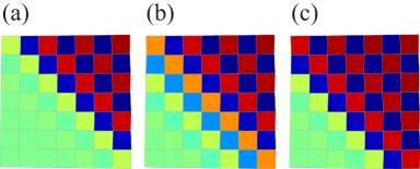
Figure 11: (Color online) Configuration of lattice distortions near the domain boundary, as the boundary moves by two interatomic distances. The color scheme is different from Figs. 4, 7, and 8(a). Here, the color represents the $s_{x}$ mode, with red, green, and blue corresponding to $s_{o}$, 0, and $-s_{o}$, respectively. (a), (b), and (c) correspond to the profile represented by red, green, and purple dots in Fig. 10. Configuration (c) has a lower energy than (a), but the higher energy of the intermediate configuration (b) serves as a Peierls-Nabarro barrier, as shown in Fig. 12.

In this section, we examine the stability of the phase coexistence against various kinds of perturbations. First, we examine the energy barrier blocking a uniform shift of the domain boundaries, which would convert the undistorted high energy phase into the distorted low energy phase. Red dots connected by the lowest lines in Fig. 10 show $s_{x}(i_{x},i_{y})\times(-1)^{i_{x}+i_{y}}$ versus $i_{x}$ for $i_{y}=1$ near the boundary between the undistorted (i.e., $i_{x}\leq 51$) and distorted (i.e., $i_{x}\geq 52$) phases for the configuration in Fig. 8(a). To find the energy barrier against uniform domain wall shift, we increase the value of $s_{x}(i_{x},i_{y})\times(-1)^{i_{x}+i_{y}}$ at the sites immediately adjacent to the domain boundary, that is, at $i_{x}=51-i_{s}$, $i_{y}=1+i_{s}$ with integer $i_{s}$’s, in 8 steps from near zero to the full distortion close to $s_{0}$. At each step, we minimize the total energy with respect to the distortions at all other sites using the Euler method. This gives rise to the distortion profiles along the horizontal direction shown in Fig. 10. The 2D configurations for the red, green, and purple dots in Fig. 10 are also shown in Figs. 11(a), 11(b), and 11(c), respectively, where the color represents $s_{x}$. The results show that $s_{x}(i_{x},i_{y})\times(-1)^{i_{x}+i_{y}}$ at $(51,1)$ and $(50,1)$ grow together, compensating $s_{x}$ distortions with opposite signs at the two neighboring sites, and the domain boundary advances by two interatomic distances.

We define the effective location of the domain boundary, $d_{db}$, according to

$$d_{db}=2\times\frac{s_{x}^{*}-0.040}{0.308-0.040},$$ (59)

where $s_{x}^{*}$ represents the value of $s_{x}(i_{x},i_{y})\times(-1)^{i_{x}+i_{y}}$ chosen at $i_{x}=51$ in Fig. 10, and 0.040 and 0.308 the values of $s_{x}^{*}$ before and after the domain wall moves by two interatomic distances. The minimized total energy $E^{\prime}_{tot}$ is plotted in Fig. 12 for $0\leq d_{db}\leq 2$, which shows the energy barrier. We compare three energies, $E_{1}=-2.946$, $E_{2}=-1.668$, and $E_{3}=-3.693$ for $d_{db}$ = 0.0, 1.0, and 2.0, which correspond to the configurations shown in Figs. 11(a), 11(b), and 11(c), respectively. Most changes in distortion occur in the $64\times 2$ plaquettes near the domain boundary, as shown in Figs. 10 and  11. Therefore, the energy difference between the two stable domain configurations for $d_{db}=$ 0.0 and 2.0 is $(E_{1}-E_{3})/128=0.0058$ per site, which agrees with the energy difference per site, 0.0058, between the undistorted and distorted uniform phases in Fig. 3(b). The energy barrier normalized for $64\times 2$ plaquettes, that is, $(E_{2}-E_{1})/128$, is 0.0100, which is of the same order of magnitude as the height of the energy barrier, $\Delta E=0.0160$, between the local and global energy minima in Fig. 3(b). From this analysis, the energy barrier against the uniform shift of the domain wall would be of the order of $2\Delta E$ multiplied by the domain wall length in the units of interatomic distance, which would be a macroscopic energy barrier for the domain walls of micron length scale. We emphasize that discreteness of the lattice in our model is essential for this energy barrier, which is an example of the Peierls-Nabarro barrier. Nabarro

III.2 Stability against non-uniform domain wall modifications

The importance of the long range interaction between strain fields is even more evident for the stability against nonuniform modification of domain walls. As an example, we convert a patch of the undistorted region in a configuration similar to Fig. 8(a), into a distorted state initially and then relax the whole lattice according to the Euler method. The initial, two intermediate, and final configurations are displayed in Fig. 13. The results show that the distortion in the converted region disappears initially except for two atomic layers [Fig. 13(c)], which shrink laterally by further relaxation, restoring the original configuration [Fig. 13(d)]. The simulation demonstrates the stability of domain structure against non-uniform modification of the domain walls. To gain further insight into the role of lattice compatibility, we examine other modes and energy distributions. Figures 14(a), 14(b) and 14(c) show the modes, $e_{1}$, $e_{2}$, and $e_{3}$ for the $s_{x}$ distortion given in Fig. 13(b). The strain field tends to spread into the domains from the domain boundary. In particular, the $e_{3}$ field inside the converted patch in Fig. 14(c) cannot reach $-C_{3}s_{0}^{2}/A_{3}$, the full distortion of $e_{3}$ inside the domain, due to the strain compatibility. The map of $E_{tot}(\vec{i})$, the sum of the terms with the site index $\vec{i}$ in Eqs. (39)-(41), is shown in Fig. 14(d), which implies that the energy cost for creating the distorted patch is not confined immediately around the interface, but is distributed over the whole converted patch. This is different from systems with short range interactions only, for which the energy cost would be confined near the domain wall within the range of the interaction. This difference shows that the lattice constraint, leading to the effective long range interaction, plays an important role in the stability of phase coexistence against non-uniform modification of the domain boundary. Similarly, we find that if we convert a patch of the distorted region of a similar size as above into the undistorted phase, the system relaxes back to the original configuration.

However, the above results do not mean that it is impossible to convert a region between phases. For example, if we convert a large enough patch, as shown in Fig. 15(a), even though the distortion in the most converted region disappears initially, the two distorted layers remaining in Fig. 15(b) expand laterally, as shown in Fig. 15(c). Eventually, the distorted domain grows by two atomic layers, as shown in Fig. 15(d). These results, particularly the different relaxation behavior for the configurations in Figs. 13(c) and 15(c), show that the energy barrier for the growth of the low energy phase involves simultaneous distortions of a significant number of unit cells just next to the domain wall. Slow growth of the low energy phase has been observed in a number of experiments for manganites. For example, Ref. Tao05, reports a time scale of the order of 10 minutes for the growth of the low energy phase. A rough order of magnitude estimate of the energy barrier $\Delta E$ can be made by assuming an activated thermal process so that the relaxation time $\tau=\tau_{0}\exp(\Delta E/k_{B}T)$, where $\tau_{0}$ represents the intrinsic time scale for ion motion, $k_{B}$ is the Boltzmann constant, and $T$ is temperature. With $\tau\sim 10^{3}$ s, $\tau_{0}\sim 10^{-13}$ s, $k_{B}T\sim 10$ meV, we obtain $\Delta E$ of the order of 1 eV. If we consider the typical energy scale for the distortion of unit cell to be 1 - 10 meV, this energy barrier corresponds to about 100 - 1000 unit cell distortions within the layer just next to the 2-dimensional interface, consistent with our simulations. A similar growth of the undistorted region occurs if we convert a large enough distorted region into the undistorted phase, as shown in Fig. 16. The result in Fig. 16 is reminiscent of experiments in which the volume fraction of the undistorted phase is increased by external perturbations such as x-rays or light. Kiryukhin97 ; Fiebig98

IV Summary

We have discussed various aspects of a model for the strain-induced phase coexistence observed in perovskite manganites. A square lattice and associated atomic scale distortion modes were used to construct an energy expression with local and global energy minimum states, which captures features of manganites essential for phase coexistence: a local energy minimum metallic state without lattice distortions and a global energy minimum insulating state with short wavelength and uniform lattice distortions. Explicit expressions for modes, constraint equations, energies, and energy gradients have been presented. Our simulations for an energy landscape with a low energy barrier against transforming from undistorted local to distorted global energy minimum states revealed nucleation with anisotropic correlation upon rapid quenching. Our simulations for an energy landscape with a high energy barrier showed stable coexistence of undistorted metallic and distorted insulating domains. Further, we studied the stability of such metal-insulator domain structures against various perturbations. We found that domain configurations are stable against uniform motion of the boundary due to the discreteness of the lattice and the intrinsic energy barrier between local and global energy minimum states. We expect that this intrinsic atomic scale energy barrier, multiplied by the number of atoms within the mesoscopic scale domain wall, is large enough to prevent the uniform motion of domain walls. For non-uniform modification of these walls, the long range interaction between strain fields gives rise to the domain wall energy distributed over the whole modified area for our 2D model (or volume for 3D system), rather than just the region confined near the domain wall, providing extra stability to the domain structure. To provide comparison, we carried out simulations for a system with a short range interaction only, which show no anisotropic nucleation or stable coexistence of local and global energy minimum phases. The above results demonstrate that the long range interaction between stain fields, and associated complex energy landscape, play an important role in metal-insulator coexistence in perovskite manganites.

Establishment of more concrete connections between our model and experiments would be the goal of future studies. For example, the density of states at the Fermi energy level in the inhomogeneous state can be compared with the conductivity measured in experiments. The effect of substrate-induced strain can be simulated in our model with additional energy terms representing the bonding between atoms in the film and the substrate. Thermal fluctuation can be simulated by the Monte Carlo method, which may provide insights into the origin of “strain” glass behavior that has been experimentally proposed as intrinsic rather than extrinsic. Wu06 Furthermore, although our framework is based on the assumption that electronic and magnetic effects are adiabatically slaved to lattice distortions, our work can, in principle, be generalized to include these functionalities in a self-consistent manner. Such coupled models will be computationally intensive and our approach has been to seek a minimal model. However, discrete strain or pseudo-spin models Lookman08 with long-range interactions and disorder provide a skeletal approach to couple with magnetic spins and electronic densities within a mean-field or Monte Carlo scheme. Here the abundant literature on spin models is an advantage because even glassy behavior in electronic materials may be identified by an appropriate order-parameter.

V Acknowledgement

We thank Avadh Saxena for discussions. This work has been supported by U.S. Department of Energy and NJIT.

Appendix A Energy expressions for inhomogeneous states

First, we represent $e_{1}$, $e_{2}$, and $e_{3}$ in the reciprocal space, and rewrite $E_{l}$ and $E_{c}$ in Eqs. (40) and (41) in the following form:

$$E_{l} = N^{2}\sum_{\vec{k}}\frac{A_{1}}{2}e_{1}(\vec{k})e_{1}(-\vec{k})+\frac{A_{2}}{2}e_{2}(\vec{k})e_{2}(-\vec{k})+\frac{A_{3}}{2}e_{3}(\vec{k})e_{3}(-\vec{k}),$$ (60)

$$E_{c} = \sum_{\vec{i}}\left\{C_{3}\left[s_{x}(\vec{i})^{2}-s_{y}(\vec{i})^{2}\right]\sum_{\vec{k}}e_{3}(\vec{k})e^{i\vec{k}\cdot\vec{i}}\right\}.$$ (61)

Next, because the constraint equations apply differently depending on whether either $k_{x}$ or $k_{y}$ is zero or not, we divide the $\vec{k}$-sum into four parts,

$$\sum_{\vec{k}}=\sum_{k_{x}\neq 0,k_{y}\neq 0}+\sum_{k_{x}=0,k_{y}\neq 0}+\sum_{k_{x}\neq 0,k_{y}=0}+\sum_{k_{x}=0,k_{y}=0},$$ (62)

and treat each of them separately. If $k_{x}\neq 0$ and $k_{y}\neq 0$, constraint equations Eqs. (25)-(27) are rewritten in the following way, which expresses the modes $e_{1}(\vec{k})$, $e_{2}(\vec{k})$, $e_{3}(\vec{k})$ in terms of $s_{x}(\vec{k})$ and $s_{y}(\vec{k})$:

$$(e_{1})_{k_{x}\neq 0,k_{y}\neq 0} = -\frac{i}{\sqrt{2}}\left[\cot\frac{k_{y}}{2}s_{x}(\vec{k})+\cot\frac{k_{x}}{2}s_{y}(\vec{k})\right],$$ (63)

$$(e_{2})_{k_{x}\neq 0,k_{y}\neq 0} = -\frac{i}{\sqrt{2}}\left[\cot\frac{k_{x}}{2}s_{x}(\vec{k})+\cot\frac{k_{y}}{2}s_{y}(\vec{k})\right],$$ (64)

$$(e_{3})_{k_{x}\neq 0,k_{y}\neq 0} = -\frac{i}{\sqrt{2}}\left[\cot\frac{k_{y}}{2}s_{x}(\vec{k})-\cot\frac{k_{x}}{2}s_{y}(\vec{k})\right].$$ (65)

Therefore, the part with $k_{x}\neq 0$ and $k_{y}\neq 0$ for $E_{l}$ in Eq. (60) is expressed as

$$(E_{l})_{k_{x}\neq 0,k_{y}\neq 0}=\frac{N^{2}}{2}\sum_{k_{x}\neq 0,k_{y}\neq 0}\left(\begin{array}[]{c}s_{x}\\ s_{y}\end{array}\right)^{T}_{-\vec{k}}\left(\begin{array}[]{cc}B_{xx}&B_{xy}\\ B_{xy}&B_{yy}\end{array}\right)_{\vec{k}}\left(\begin{array}[]{c}s_{x}\\ s_{y}\end{array}\right)_{\vec{k}},$$ (66)

where

$$B_{xx}(\vec{k}) = \frac{1}{2}(A_{1}+A_{3})\cot^{2}\frac{k_{y}}{2}+\frac{1}{2}A_{2}\cot^{2}\frac{k_{x}}{2},$$ (67)

$$B_{yy}(\vec{k}) = \frac{1}{2}(A_{1}+A_{3})\cot^{2}\frac{k_{x}}{2}+\frac{1}{2}A_{2}\cot^{2}\frac{k_{y}}{2},$$ (68)

$$B_{xy}(\vec{k}) = \frac{1}{2}(A_{1}+A_{2}-A_{3})\cot\frac{k_{x}}{2}\cot\frac{k_{y}}{2}.$$ (69)

Similarly, the part with $k_{x}\neq 0$ and $k_{y}\neq 0$ for $E_{c}$ in Eq. (61) is equivalent to

$$(E_{c})_{k_{x}\neq 0,k_{y}\neq 0}=\sum_{\vec{i}}C_{3}\left[s_{x}(\vec{i})^{2}-s_{y}(\vec{i})^{2}\right]\sum_{k_{x}\neq 0,k_{y}\neq 0}-\frac{i}{\sqrt{2}}\left[\cot\frac{k_{y}}{2}s_{x}(\vec{k})-\cot\frac{k_{x}}{2}s_{y}(\vec{k})\right]e^{i\vec{k}\cdot\vec{i}}.$$ (70)

For the terms with $k_{x}=0$ and $k_{y}\neq 0$, we apply the constraint equation $e_{1}(\vec{k})+e_{3}(\vec{k})=0$ to eliminate $e_{1}(\vec{k})$ in $E_{l}$ in Eq. (60) and obtain

$$(E_{l}+E_{c})_{k_{x}=0,k_{y}\neq 0} = N^{2}\sum_{k_{x}=0,k_{y}\neq 0}\frac{1}{2}(A_{1}+A_{3})e_{3}(-\vec{k})e_{3}(\vec{k})+\frac{1}{2}A_{2}e_{2}(-\vec{k})e_{2}(\vec{k})$$ (71)

$$+\sum_{\vec{i}}C_{3}\left[s_{x}(\vec{i})^{2}-s_{y}(\vec{i})^{2}\right]\sum_{k_{x}=0,k_{y}\neq 0}e_{3}(\vec{k})e^{ik_{y}i_{y}}.$$

Since we are interested in metastable phases in this work and $e_{2}(\vec{k})$ and $e_{3}(\vec{k})$ are independent for $k_{x}=0$ and $k_{y}\neq 0$, we minimize the energy $(E_{l}+E_{c})_{k_{x}=0,k_{y}\neq 0}$ with respect to $e_{2}(\vec{k})$ and $e_{3}(\vec{k})$ separately and obtain

$$(e_{1})^{min}_{k_{x}=0,k_{y}\neq 0}=-(e_{3})^{min}_{k_{x}=0,k_{y}\neq 0}=\frac{C_{3}}{A_{1}+A_{3}}\mathcal{F}_{0,k_{y}}(s_{x}^{2}-s_{y}^{2}),$$ (72)

$$(e_{2})^{min}_{k_{x}=0,k_{y}\neq 0}=0,$$ (73)

where

$$\mathcal{F}_{\vec{k}}(s_{x}^{2}-s_{y}^{2})\equiv\frac{1}{N^{2}}\sum_{\vec{i}}\left[s_{x}(\vec{i})^{2}-s_{y}(\vec{i})^{2}\right]e^{-i\vec{k}\cdot\vec{i}}.$$ (74)

The minimized energy expression for $(E_{l}+E_{c})_{k_{x}=0,k_{y}\neq 0}$ is

$$(E_{l}+E_{c})^{min}_{k_{x}=0,k_{y}\neq 0}=-\frac{C_{3}^{2}}{2(A_{1}+A_{3})}N^{2}\sum_{k_{x}=0,k_{y}\neq 0}\mathcal{F}_{0,-k_{y}}(s_{x}^{2}-s_{y}^{2})\mathcal{F}_{0,k_{y}}(s_{x}^{2}-s_{y}^{2}).$$ (75)

We apply a similar analysis for the terms with $k_{x}\neq 0$ and $k_{y}=0$ in Eqs. (60) and (61). Using the constraint $e_{1}(\vec{k})-e_{3}(\vec{k})=0$, we eliminate $e_{1}(\vec{k})$ and obtain

$$(E_{l}+E_{c})_{k_{x}\neq 0,k_{y}=0} = N^{2}\sum_{k_{x}\neq 0,k_{y}=0}\frac{1}{2}(A_{1}+A_{3})e_{3}(-\vec{k})e_{3}(\vec{k})+\frac{1}{2}A_{2}e_{2}(-\vec{k})e_{2}(\vec{k})$$ (76)

$$+\sum_{\vec{i}}C_{3}\left[s_{x}(\vec{i})^{2}-s_{y}(\vec{i})^{2}\right]\sum_{k_{x}\neq 0,k_{y}=0}e_{3}(\vec{k})e^{ik_{x}i_{x}}.$$

Separate minimization of this energy with respect to $e_{2}(\vec{k})$ and $e_{3}(\vec{k})$ leads to

$$(e_{1})^{min}_{k_{x}\neq 0,k_{y}=0} = (e_{3})^{min}_{k_{x}\neq 0,k_{y}=0}=-\frac{C_{3}}{A_{1}+A_{3}}\mathcal{F}_{k_{x},0}(s_{x}^{2}-s_{y}^{2}),$$ (77)

$$(e_{2})^{min}_{k_{x}\neq 0,k_{y}=0} = 0,$$ (78)

$$(E_{l}+E_{c})^{min}_{k_{x}\neq 0,k_{y}=0} = -\frac{C_{3}^{2}}{2(A_{1}+A_{3})}N^{2}\sum_{k_{x}\neq 0,k_{y}=0}\mathcal{F}_{-k_{x},0}(s_{x}^{2}-s_{y}^{2})\mathcal{F}_{k_{x},0}(s_{x}^{2}-s_{y}^{2}).$$ (79)

The terms with $\vec{k}=0$ in Eqs. (60) and (61) are

$$(E_{l}+E_{c})_{k_{x}=0,k_{y}=0} = N^{2}\left[\frac{A_{1}}{2}e_{1}(\vec{k}=0)^{2}+\frac{A_{2}}{2}e_{2}(\vec{k}=0)^{2}+\frac{A_{3}}{2}e_{3}(\vec{k}=0)^{2}\right]$$ (80)

$$+\sum_{\vec{i}}C_{3}\left[s_{x}(\vec{i})^{2}-s_{y}(\vec{i})^{2}\right]e_{3}(\vec{k}=0).$$

We minimize the above expression with respect to $e_{1}(\vec{k}=0)$, $e_{2}(\vec{k}=0)$, and $e_{3}(\vec{k}=0)$ independently, since they are not constrained to each other, and obtain

$$(e_{1})^{min}_{k_{x}=0,k_{y}=0} = 0,$$ (81)

$$(e_{2})^{min}_{k_{x}=0,k_{y}=0} = 0,$$ (82)

$$(e_{3})^{min}_{k_{x}=0,k_{y}=0} = -\frac{C_{3}}{A_{3}}\mathcal{F}_{\vec{k}=0}(s_{x}^{2}-s_{y}^{2}),$$ (83)

$$(E_{l}+E_{c})^{min}_{k_{x}=0,k_{y}=0} = -\frac{C_{3}^{2}}{2A_{3}}N^{2}\left[\mathcal{F}_{\vec{k}=0}(s_{x}^{2}-s_{y}^{2})\right]^{2}.$$ (84)

Finally, by adding the terms with different cases of $k_{x}$ and $k_{y}$ found above, we obtain the following total energy, $E^{\prime}_{tot}$, which depends only on $s_{x}$ and $s_{y}$:

$$E^{\prime}_{tot}(s_{x},s_{y})=E^{\prime}_{l+c}+E_{s},$$ (85)

where

$$E^{\prime}_{l+c} = (E_{l})_{k_{x}\neq 0,k_{y}\neq 0}+(E_{c})_{k_{x}\neq 0,k_{y}\neq 0}+(E_{l}+E_{c})^{min}_{k_{x}\neq 0,k_{y}=0}+(E_{l}+E_{c})^{min}_{k_{x}=0,k_{y}\neq 0}$$ (86)

$$+(E_{l}+E_{c})^{min}_{k_{x}=0,k_{y}=0},$$

and $E_{s}$ is given by Eq. (39). We use this energy expression $E^{\prime}_{tot}(s_{x},s_{y})$ for the simulations of inhomogeneous states.

In addition to $s_{x}(\vec{i})$ and $s_{y}(\vec{i})$ configurations, $e_{1}(\vec{i})$, $e_{2}(\vec{i})$, and $e_{3}(\vec{i})$ configurations give useful information on the nature of the inhomogeneous states. The relations used to eliminate $e_{1}$, $e_{2}$, and $e_{3}$ variables above, namely, Eqs. (63)-(65), (72), (73), (77), (78) and (81)-(83) for different cases of $k_{x}$ and $k_{y}$, are used to find $e_{1}(\vec{k})$, $e_{2}(\vec{k})$, and $e_{3}(\vec{k})$ from given $s_{x}(\vec{i})$ and $s_{y}(\vec{i})$, which lead to $e_{1}(\vec{i})$, $e_{2}(\vec{i})$, and $e_{3}(\vec{i})$ configurations. Equations (28)-(37) are used to find the displacements, $u_{x}(\vec{i})$ and $u_{y}(\vec{i})$, from the distortion modes.

Appendix B Gradients of the energy expression for simulations using Euler method

The gradient of $E^{\prime}_{tot}(s_{x},s_{y})$ necessary for the Euler method is found from

$$\frac{\partial E^{\prime}_{tot}(s_{x},s_{y})}{\partial s_{x}(\vec{i})} = \frac{\partial(E_{l})_{k_{x}\neq 0,k_{y}\neq 0}}{\partial s_{x}(\vec{i})}+\frac{\partial(E_{c})_{k_{x}\neq 0,k_{y}\neq 0}}{\partial s_{x}(\vec{i})}+\frac{\partial(E_{l}+E_{c})^{min}_{k_{x}=0,k_{y}\neq 0}}{\partial s_{x}(\vec{i})}$$ (87)

$$+\frac{\partial(E_{l}+E_{c})^{min}_{k_{x}\neq 0,k_{y}=0}}{\partial s_{x}(\vec{i})}+\frac{\partial(E_{l}+E_{c})^{min}_{k_{x}=0,k_{y}=0}}{\partial s_{x}(\vec{i})}+\frac{\partial E_{s}}{\partial s_{x}(\vec{i})},$$

$$\frac{\partial E^{\prime}_{tot}(s_{x},s_{y})}{\partial s_{y}(\vec{i})} = \frac{\partial(E_{l})_{k_{x}\neq 0,k_{y}\neq 0}}{\partial s_{y}(\vec{i})}+\frac{\partial(E_{c})_{k_{x}\neq 0,k_{y}\neq 0}}{\partial s_{y}(\vec{i})}+\frac{\partial(E_{l}+E_{c})^{min}_{k_{x}=0,k_{y}\neq 0}}{\partial s_{y}(\vec{i})}$$ (88)

$$+\frac{\partial(E_{l}+E_{c})^{min}_{k_{x}\neq 0,k_{y}=0}}{\partial s_{y}(\vec{i})}+\frac{\partial(E_{l}+E_{c})^{min}_{k_{x}=0,k_{y}=0}}{\partial s_{y}(\vec{i})}+\frac{\partial E_{s}}{\partial s_{y}(\vec{i})}.$$

The expression for each term is given below.

$$\frac{\partial(E_{l})_{k_{x}\neq 0,k_{y}\neq 0}}{\partial s_{x}(\vec{i})} = \sum_{k_{x}\neq 0,k_{y}\neq 0}[{B}_{xx}(\vec{k})s_{x}(\vec{k})+{B}_{xy}(\vec{k})s_{y}(\vec{k})]e^{i\vec{k}\cdot\vec{i}}$$ (89)

$$\frac{\partial(E_{l})_{k_{x}\neq 0,k_{y}\neq 0}}{\partial s_{y}(\vec{i})} = \sum_{k_{x}\neq 0,k_{y}\neq 0}[{B}_{yy}(\vec{k})s_{y}(\vec{k})+{B}_{xy}(\vec{k})s_{x}(\vec{k})]e^{i\vec{k}\cdot\vec{i}}$$ (90)

$$\frac{\partial(E_{c})_{k_{x}\neq 0,k_{y}\neq 0}}{\partial s_{x}(\vec{i})} = -C_{3}\sum_{k_{x}\neq 0,k_{y}\neq 0}\frac{-i}{\sqrt{2}}\cot\frac{k_{y}}{2}\mathcal{F}_{\vec{k}}(s_{x}^{2}-s_{y}^{2})e^{i\vec{k}\cdot\vec{i}}$$ (91)

$$+2C_{3}s_{x}(\vec{i})\sum_{k_{x}\neq 0,k_{y}\neq 0}\frac{-i}{\sqrt{2}}\left[\cot\frac{k_{y}}{2}s_{x}(\vec{k})-\cot\frac{k_{x}}{2}s_{y}(\vec{k})\right]e^{i\vec{k}\cdot\vec{i}}$$

$$\frac{\partial(E_{c})_{k_{x}\neq 0,k_{y}\neq 0}}{\partial s_{y}(\vec{i})} = -C_{3}\sum_{k_{x}\neq 0,k_{y}\neq 0}\frac{-i}{\sqrt{2}}\cot\frac{k_{x}}{2}\mathcal{F}_{\vec{k}}(s_{y}^{2}-s_{x}^{2})e^{i\vec{k}\cdot\vec{i}}$$ (92)

$$+2C_{3}s_{y}(\vec{i})\sum_{k_{x}\neq 0,k_{y}\neq 0}\frac{-i}{\sqrt{2}}\left[\cot\frac{k_{x}}{2}s_{y}(\vec{k})-\cot\frac{k_{y}}{2}s_{x}(\vec{k})\right]e^{i\vec{k}\cdot\vec{i}}$$

$$\frac{\partial(E_{l}+E_{c})^{min}_{k_{x}=0,k_{y}\neq 0}}{\partial s_{x}(\vec{i})} = -\frac{2C_{3}^{2}}{A_{1}+A_{3}}s_{x}(\vec{i})\sum_{k_{x}=0,k_{y}\neq 0}e^{ik_{y}i_{y}}\mathcal{F}_{0,k_{y}}(s_{x}^{2}-s_{y}^{2})$$ (93)

$$\frac{\partial(E_{l}+E_{c})^{min}_{k_{x}=0,k_{y}\neq 0}}{\partial s_{y}(\vec{i})} = \frac{2C_{3}^{2}}{A_{1}+A_{3}}s_{y}(\vec{i})\sum_{k_{x}=0,k_{y}\neq 0}e^{ik_{y}i_{y}}\mathcal{F}_{0,k_{y}}(s_{x}^{2}-s_{y}^{2})$$ (94)

$$\frac{\partial(E_{l}+E_{c})^{min}_{k_{x}\neq 0,k_{y}=0}}{\partial s_{x}(\vec{i})} = -\frac{2C_{3}^{2}}{A_{1}+A_{3}}s_{x}(\vec{i})\sum_{k_{x}\neq 0,k_{y}=0}e^{ik_{x}i_{x}}\mathcal{F}_{k_{x},0}(s_{x}^{2}-s_{y}^{2})$$ (95)

$$\frac{\partial(E_{l}+E_{c})^{min}_{k_{x}\neq 0,k_{y}=0}}{\partial s_{y}(\vec{i})} = \frac{2C_{3}^{2}}{A_{1}+A_{3}}s_{y}(\vec{i})\sum_{k_{x}\neq 0,k_{y}=0}e^{ik_{x}i_{x}}\mathcal{F}_{k_{x},0}(s_{x}^{2}-s_{y}^{2})$$ (96)

$$\frac{\partial(E_{l}+E_{c})^{min}_{\vec{k}=0}}{\partial s_{x}(\vec{i})} = -\frac{2C_{3}^{2}}{A_{3}}s_{x}(\vec{i})\mathcal{F}_{\vec{k}=0}(s_{x}^{2}-s_{y}^{2})$$ (97)

$$\frac{\partial(E_{l}+E_{c})^{min}_{\vec{k}=0}}{\partial s_{y}(\vec{i})} = \frac{2C_{3}^{2}}{A_{3}}s_{y}(\vec{i})\mathcal{F}_{\vec{k}=0}(s_{x}^{2}-s_{y}^{2})$$ (98)

$$\frac{\partial E_{s}}{\partial s_{x}(\vec{i})} = Bs_{x}(\vec{i})+G_{1}s_{x}(\vec{i})^{3}+G_{2}s_{x}(\vec{i})s_{y}(\vec{i})^{2}+H_{1}s_{x}(\vec{i})^{5}$$ (99)

$$+\frac{H_{2}}{3}\left[2s_{x}(\vec{i})^{2}+s_{y}(\vec{i})^{2}\right]s_{x}(\vec{i})s_{y}(\vec{i})^{2}$$

$$\frac{\partial E_{s}}{\partial s_{y}(\vec{i})} = Bs_{y}(\vec{i})+G_{1}s_{y}(\vec{i})^{3}+G_{2}s_{x}(\vec{i})^{2}s_{y}(\vec{i})+H_{1}s_{y}(\vec{i})^{5}$$ (100)

$$+\frac{H_{2}}{3}\left[2s_{y}(\vec{i})^{2}+s_{x}(\vec{i})^{2}\right]s_{y}(\vec{i})s_{x}(\vec{i})^{2}$$

Figure 1: Two-dimensional square lattice with a monatomic basis. $\vec{u}_{\vec{i}}$ represents the displacement of the atom at the site with the index $\vec{i}=(i_{x},i_{y})$, where integer $i_{x}$ and $i_{y}$ range from 1 to $N$. The site at the bottom left corner is chosen for $\vec{i}=(1,1)$. In this work, the lattice constant $a$ is irrelevant for the expressions of modes and energies, and can be chosen arbitrarily, so long as the sequence of the atoms is not changed by the displacements. For figures in this work, $a$ is chosen as 10, but the result itself is independent of the choice of $a$.

Figure 2: Symmetry distortion modes Ahn03 for the motif for the two-dimensional square lattice with a monatomic basis shown in Fig. 1.

Figure 4: (Color online) Simulation of lattice relaxation for a $32\times 32$ lattice for the energy landscape with a shallow local minimum, namely the thin blue curve in Fig. 3(b). The vertices correspond to the positions of atoms and actual distortions are shown. The color represents $p_{3}=s_{x}^{2}-s_{y}^{2}$, green corresponding to zero, red and blue $\pm s_{0}^{2}$, except $\pm(2.6s_{0})^{2}$ for the panel (a). The dynamics is governed by the Euler method, simulating a rapid quenching from a random initial configuration shown in (a). (b)-(g) show intermediate configurations and (h) the final stable configuration, in which most region is changed to distorted state except the antiphase boundaries represented in green. Highly anisotropic nucleation and the effect of long range interaction can be identified, for example, in (d) and (e).

Figure 5: (Color online) Simulation of relaxation for a system with a short range interaction only. The variable $p=M^{2}$ is plotted on a $32\times 32$ lattice with a periodic boundary condition. Red represents $p=28.6M_{0}^{2}$ for (a) and $p=M_{0}^{2}$ for (b)-(h), and green $p=0$. A random initial configuration is shown in (a). (b)-(g) show intermediate configurations, and (h) the final stable configuration. The result shows that nucleation for short range interaction is nearly isotropic, unlike the case in Fig. 4.

Figure 6: (Color online) (a) Map of local electron DOS at $E=0$ calculated for the distortion shown in Fig. 4(f). Blue, green, and red correspond to zero, 0.25, and 0.5 state per site per unit energy, respectively. (b) Local DOS calculated at $\vec{i}=(17,10)$, the center of an undistorted metallic region, and at $\vec{i}=(7,9)$, center of a distorted insulating region. It shows coexistence of metallic and insulating regions.

Figure 7: (Color online) Simulation of relaxation of lattice distortions for random initial distortions in a narrower range compared to the case in Fig. 4. Color scheme is identical to Fig. 4. The initial configuration in (a) is obtained by multiplying 0.5 to the random initial $s_{x}(\vec{i})$ and $s_{y}(\vec{i})$ in Fig. 4(a). The comparison with Fig. 4 indicates that the low temperature phase depends on how the system is prepared, as observed in some manganites.

Figure 8: (Color online) (a) Stable configuration of distorted and undistorted domains for a $64\times 64$ lattice for the energy landscape with a deep local minimum, shown by the thick red curve in Fig. 3(b). The color represents $p_{3}$ with red and green for $s_{o}^{2}$ and 0, respectively. (b) Map of the local electron DOS calculated at $E=0$ for the distortions in (a). Red, green, and blue correspond to 0.6, 0.3, and 0 state per site per energy, respectively. There is no intrinsic length scale for the size of the domains in our model, and the size of the domain depends only on the predesigned initial condition and can be as large as micron in principle, which is consistent with experimental observations.

Figure 12: Total energy $E^{\prime}_{tot}$ for the 64 $\times$ 64 system, given by Eq. (85), versus the location of the domain boundary defined by Eq. (59), as the boundary moves by two interatomic distances. Each point is found from each corresponding curve in Fig. 10. The configurations in Figs. 11(a), 11(b), and 11(c) correspond to $d_{db}=0.0$, 1.0, and 2.0, respectively. The energy barrier prevents a parallel shift of the domain wall.

Figure 13: (Color online) Simulation of the domain wall stability against a small nonuniform modification of the domain boundary for the configuration similar to Fig. 8(a). The color scheme is identical to Fig. 11. (a) represents the initial perturbed configuration. (b) and (c) show intermediate configurations. (d) represents the final stable configuration, which is identical to the original configuration before the perturbation. It shows that the original domain configuration, such as the one shown in Fig. 8, is stable against small non-parallel shift of the domain boundary.

Figure 14: (Color online) Colors in (a), (b) and (c) show the $e_{1}(\vec{i})$, $e_{2}(\vec{i})$, and $e_{3}(\vec{i})$ for the configuration shown in Fig. 13(b). Colors in (d) show $E_{tot}(\vec{i})$, which is the sum of the terms with the site index $\vec{i}$ in Eqs. (39)-(41). In the panels (a), (b), and (c), red and blue correspond to $\pm 0.45$ and green to zero. In the panel (d), red and blue correspond to 0.06 and -0.006, respectively. Typical values of $e_{3}(\vec{i})$ and $E_{tot}(\vec{i})$ inside the converted patch are -0.08 and 0.02, respectively. Panel (d) shows that the energy cost for changing domain wall in a non-parallel way spreads over the whole changed area (volume in 3D), which is different from systems with a short range interaction only and is responsible for the stability against such non-parallel shift of the domain walls.

Figure 15: (Color online) Simulation of the domain wall shift by large enough nonuniform modification of the domain boundary, converting a large undistorted patch into a distorted state, for the configuration similar to Fig. 8(a). The color scheme is identical to Fig. 11. An initial configuration is shown in (a). (b) and (c) show intermediate configurations. (d) represents the final stable configuration, which shows that the distorted region has expanded by two atomic layers. It shows that if the perturbation is large enough, the system relaxes to a different metastable configuration, unlike the case in Fig. 13.

Figure 16: (Color online) Simulation of the domain wall shift by a large enough nonuniform modification of the domain boundary, converting a large distorted patch into an undistorted state, for the configuration similar to Fig. 8(a). The color scheme is identical to Fig. 11. An initial configuration is shown in (a). (b) and (c) show intermediate configurations. (d) represents the final stable configuration, which shows that the undistorted metallic region has expanded. This simulation may be related to the experiment results in Ref. Kiryukhin97, , in which the x-rays destroy the charge-orbital ordering and the short wavelength distortions and increase conductivity.

References

• (1) M. B. Salamon and M. Jaime, Rev. Mod. Phys. 73, 583 (2001).
• (2) M. Uehara, S. Mori, C. H. Chen, and S.-W. Cheong, Nature (London) 399, 560 (1999).
• (3) Ch. Renner, G. Aeppli, B.-G. Kim, Y.-A. Soh, and S.-W. Cheong, Nature (London) 416, 518 (2002).
• (4) M. Fäth, S. Freisem, A. A. Menovsky, Y. Tomioka, J. Aarts, and J. A. Mydosh, Science 285, 1540 (1999).
• (5) V. Kiryukhin, New J. Phys. 6 155, 1 (2004).
• (6) A. Moreo, S. Yunoki, and E. Dagotto, Science 283, 2034 (1999).
• (7) J. Burgy, A. Moreo, and E. Dagotto, Phys. Rev. Lett. 92, 097202 (2004).
• (8) K. H. Ahn and T. Lookman, cond-mat/0408077.
• (9) K. H. Ahn, T. Lookman, and A. R. Bishop, Nature (London) 428, 401 (2004).
• (10) N. D. Mathur and P. B. Littlewood, Solid State Commun. 119, 271 (2001).
• (11) A. J. Millis, Solid State Commun. 126, 3 (2003).
• (12) A. R. Bishop, T. Lookman, A. Saxena, and S. R. Shenoy, Europhys. Lett. 63, 289 (2003).
• (13) N. Mathur and P. Littlewood, Nature Mater. 3, 207 (2004).
• (14) D. D. Sarma, D. Topwal, U. Manju, S. R. Krishnakumar, M. Bertolo, S. La Rosa, G. Cautero, T. Y. Koo, P. A. Sharma, S.-W. Cheong, and A. Fujimori, Phys. Rev. Lett. 93, 097202 (2004).
• (15) J. Tao, D. Niebieskikwiat, M. B. Salamon, and J. M. Zuo, Phys. Rev. Lett. 94, 147206 (2005).
• (16) T. Z. Ward, J. D. Budai, Z. Gai, J. Z. Tischler, L. Yin, and J. Shen, Nature Phys. 5, 885 (2009).
• (17) N. Mathur and P. Littlewood, Phys. Today 56, 25 (2003).
• (18) A. J. Millis, Nature (London) 392, 147 (1998).
• (19) S. Jin, T. H. Tiefel, M. McCormack, R. A. Fastnacht, R. Ramesh, and L. H. Chen, Science 264, 413 (1994).
• (20) C. H. Chen and S.-W. Cheong, Phys. Rev. Lett. 76, 4042 (1996).
• (21) Y. Tokura, H. Kuwahara, Y. Moritomo, Y. Tomioka, and A. Asamitsu, Phys. Rev. Lett. 76, 3184 (1996).
• (22) H. Y. Hwang, S.-W. Cheong, P. G. Radaelli, M. Marezio, and B. Batlogg, Phys. Rev. Lett. 75, 914 (1995).
• (23) H. Y. Hwang, T. T. M. Palstra, S.-W. Cheong, and B. Batlogg, Phys. Rev. B 52, 15046 (1995).
• (24) V. Kiryukhin, D. Casa, J. P. Hill, B. Keimer, A. Vigliante, Y. Tomioka, and Y. Tokura, Nature (London) 386, 813 (1997).
• (25) V. Podzorov, B. G. Kim, V. Kiryukhin, M. E. Gershenson, and S.-W. Cheong, Phys. Rev. B 64, 140406 (2001).
• (26) T. Lookman, S. R. Shenoy, K. Ø. Rasmussen, A. Saxena, and A. R. Bishop, Phys. Rev. B 67, 024114 (2003); T. Lookman and P. B. Littlewood, MRS Bull. 34, 822 (2009).
• (27) S. R. Shenoy, T. Lookman, A. Saxena, and A. R. Bishop, Phys. Rev. B 60, R12537 (1999).
• (28) K. H. Ahn, T. Lookman, A. Saxena, and A. R. Bishop, Phys. Rev. B 68, 092101 (2003).
• (29) X. Ren and K. Otsuka, MRS Bull. 27, 115 (2002).
• (30) K. Ø. Rasmussen, T. Lookman, A. Saxena, A. R. Bishop, R. C. Albers, and S. R. Shenoy, Phys. Rev. Lett. 87, 055704 (2001).
• (31) We note that because of the anisotropy, e.g. $cos(4\theta)$ in 2D in Ref. Shenoy99, , the interaction is more convergent than for $1/r^{D}$.
• (32) K. H. Ahn, T. Lookman, A. Saxena, and A. R. Bishop, Phys. Rev. B 71, 212102 (2005).
• (33) N. Poccia, A. Ricci, and A. Bianconi, J. Supercond. Nov. Magn. 24, 1195 (2011).
• (34) Small mistake has been found in the code used in Ref. Ahn04, , which was corrected here, responsible for minor differences between Figs. 4(a)-4(g) and the corresponding figures in Ref. Ahn04, . The difference in Fig. 4(h) is because the simulation in Ref. Ahn04, was stopped when the energy change is considered as sufficiently small, not when the energy change fluctuates, which is used as condition for the final stability in current Euler simulations.
• (35) H. Seto, Y. Noda, and Y. Yamada, J. Phys. Soc. Jpn. 59, 978 (1990).
• (36) J. W. Lynn, R. W. Erwin, J. A. Borchers, Q. Huang, A. Santoro, J-L. Peng, and Z. Y. Li, Phys. Rev. Lett. 76, 4046 (1996).
• (37) J. W. Lynn, R. W. Erwin, J. A. Borchers, A. Santoro, Q. Huang, J.-L. Peng, and R. L. Greene, J. Appl. Phys. 81, 5488 (1997).
• (38) K. H. Kim, M. Uehara, and S.-W. Cheong, Phys. Rev. B 62, R11945 (2000).
• (39) H. J. Lee, K. H. Kim, M. W. Kim, T. W. Noh, B. G. Kim, T. Y. Koo, S.-W. Cheong, Y. J. Wang, and X. Wei, Phys. Rev. B 65, 115118 (2002).
• (40) W. Wu, C. Israel, N. Hur, S. Park, S.-W. Cheong, and A. de Lozanne, Nature Mater. 5, 881 (2006).
• (41) M. Fiebig, K. Miyano, Y. Tomioka, and Y. Tokura, Science 280, 1925 (1998).
• (42) F. Nabarro, in Theory of Crystal Dislocations (Clarendon, Oxford, 1967).
• (43) S.R. Shenoy and T. Lookman, Phys. Rev. B 78, 144103 (2008); R. Vasseur and T. Lookman, Phys. Rev. B 81, 094107 (2010); R. Vasseur and T. Lookman, Solid State Phenom. 172-174, 1078 (2011).
Refer to caption