Anisotropic Norm Bounded Real Lemma for Linear Discrete Time Varying Systems

Abstract

We consider a finite horizon linear discrete time varying system whose input is a random noise with an imprecisely known probability law. The statistical uncertainty is described by a nonnegative parameter $a$ which constrains the anisotropy of the noise as an entropy theoretic measure of deviation of the actual noise distribution from Gaussian white noise laws with scalar covariance matrices. The worst-case disturbance attenuation capabilities of the system with respect to the statistically uncertain random inputs are quantified by the $a$-anisotropic norm which is a constrained operator norm of the system. We establish an anisotropic norm bounded real lemma which provides a state-space criterion for the $a$-anisotropic norm of the system not to exceed a given threshold. The criterion is organized as an inequality on the determinants of matrices associated with a difference Riccati equation and extends the Bounded Real Lemma of the ${\mathcal{H}}_{\infty}$-control theory. We also provide a necessary background on the anisotropy-based robust performance analysis.

1 Introduction

The statistical uncertainty, present in random disturbances as a discrepancy between the imprecisely known true probability distribution of the noise and its nominal model, may corrupt the expected performance of a stochastic control system if the controller design is oriented at a specific probability law of the disturbance. Such uncertainties result not only from the lack of prior knowledge of the actual noise statistics, but also from the inherent variability of the environment where the control system operates.

The robustness in stochastic control can therefore be achieved by explicitly incorporating different scenarios of the noise distribution into a single performance index to be optimized. The degree of robustness depends on the “size” of the uncertainty used in the controller design. The statistical uncertainty can be measured in entropy theoretic terms and the robust performance index can be chosen so as to quantify the worst-case disturbance attenuation capabilities of the system. It is this combination of approaches that underlies the anisotropy-based theory of stochastic robust control which was initiated about sixteen years ago at the interface of the entropy/information and robust control theories in a series of papers (Semyonov et al. (1994); Vladimirov et al. (1995a, b, 1996a, 1996b, 1999)). This theory employs the anisotropy functional as an entropy theoretic measure of deviation of the unknown actual noise distribution from the family of Gaussian white noise laws with scalar covariance matrices. Accordingly, the role of a robust performance index is played by the $a$-anisotropic norm ${|\!|\!|}F{|\!|\!|}_{a}$ of a system $F$ which is defined as the largest ratio of the root mean square (RMS) value of the output of the system to that of the input, provided that the anisotropy of the input disturbance does not exceed a given nonnegative parameter $a$. Thus, the input anisotropy level $a$ is the size of the statistical uncertainty, and the $a$-anisotropic norm of the system ${|\!|\!|}F{|\!|\!|}_{a}$ is the worst-case RMS gain which, in the framework of the disturbance attenuation paradigm, is to be minimized.

An important property of the $a$-anisotropic norm is that it coincides with a rescaled Frobenius (or ${\mathcal{H}}_{2}$) norm of the system for $a=0$ and converges to the induced (or ${\mathcal{H}}_{\infty}$) norm as $a\to+\infty$. Therefore, ${|\!|\!|}\cdot{|\!|\!|}_{a}$ is an anisotropy-constrained stochastic version of the induced norm of the system which occupies a unifying intermediate position between the ${\mathcal{H}}_{2}$ and ${\mathcal{H}}_{\infty}$-norms utilised as performance criteria in the linear quadratic Gaussian (LQG) (Kwakernaak & Sivan (1972)) and ${\mathcal{H}}_{\infty}$-control theories (Doyle et al. (1989)).

In its original infinite horizon time invariant setting, the anisotropy-based theory employed the anisotropy production rate per time step in a stationary Gaussian random sequence. The mean anisotropy has useful links with the condition number of the covariance matrix and the transient time in the sequence, thus describing the amount of spatial non-roundness and temporal correlation in it. These connections have recently been revisited in (Kurdyukov & Vladimirov (2008)).

At the performance analysis level, the anisotropy-based theory was developed for time invariant systems in (Vladimirov et al. (1996a)), where equations were obtained for computing the $a$-anisotropic norm in state space. An extended exposition of that work can be found in (Diamond et al. (2001)) and a generalization to finite horizon time varying systems is provided by (Vladimirov et al. (2006)).

A state-space solution to the anisotropy-based optimal control problem (which seeks an internally stabilizing controller to minimize the $a$-anisotropic norm of the closed-loop system) was obtained in (Vladimirov et al. (1996b)). The solution was found as a saddle point in the stochastic minimax problem. The anisotropy-based theory therefore offers tools both for the quantitative description of uncertainty and robust performance analysis on the one hand, and control design on the other.

The present paper is concerned with the anisotropy-based robust performance analysis of linear discrete time varying (LDTV) systems in state space. The procedure developed in (Vladimirov et al. (2006)) for computing the $a$-anisotropic norm of such a system over a finite time horizon involves the solution of three coupled equations: a backward difference Riccati equation, a forward difference Lyapunov equation, and an algebraic equation for the determinants of matrices associated with the previous equations. Its practical implementation is complicated by the opposite time ordering of the coupled difference equations.

Here, we develop an alternative state-space criterion for the $a$-anisotropic norm to be bounded by a given threshold. This allows the above issue to be overcome by eliminating the Lyapunov equation, replacing the backward Riccati equation by a forward Riccati equation, and replacing the algebraic equation by an appropriately modified inequality. The resulting Anisotropic Norm Bounded Real Lemma (ANBRL) is organised as an inequality on matrices associated with a forward difference Riccati equation. In addition to a significant simplification of the previously developed anisotropy-based robust performance analysis (which can now be carried out recursively in time), ANBRL also provides an extension of the Bounded Real Lemma from the ${\mathcal{H}}_{\infty}$-control theory to the uncertain stochastic setting with finite horizon time varying dynamics. An infinite-horizon version of ANBRL for time invariant systems, which involve algebraic equations free from the opposite time ordering issue, is presented in (Kurdyukov et al. (2010)).

Another approach to robust control in stochastic systems, using the relative entropy to describe statistical uncertainty, can be found in (Petersen et al. (2000); Petersen (2006); Ugrinovskii & Petersen (2002)), where an important role is played by a link between a relative entropy duality relation and robust properties of risk-sensitive controllers (Dupuis et al. (2000)) which minimize the expected-exponential-of-quadratic functional. Although the ideas of entropy-constrained induced norms and associated stochastic minimax find further development in the control literature (Charalambous & Rezaei (2007)), the anisotropy-based theory of stochastic robust control remains largely unnoticed. It is partly for this reason that the main result of the present paper is preceded by the background material to assist the readers to build awareness of the anisotropy-based approach.

The paper is organised as follows. Section 2 specifies the class of systems being considered. Sections 3 and 4 provide the necessary background on the anisotropy of random vectors and the $a$-anisotropic norm of matrices. Section 5 establishes the Anisotropic Norm Bounded Real Lemma. Its connection with the Bounded Real Lemma in the limit $a\to+\infty$ is discussed in Section 6. Section 7 gives concluding remarks. Appendix provides a subsidiary state space criterion of outerness.

2 Class of systems being considered

We consider a linear discrete time varying (LDTV) system $F$ on a bounded time interval $[0,N]$. Its $n$-dimensional state $x_{k}$ and $r$-dimensional output $z_{k}$ at time $k$ are governed by the equations

$$x_{k+1} = A_{k}x_{k}+B_{k}w_{k},$$ (1)

$$z_{k} = C_{k}x_{k}+D_{k}w_{k},$$ (2)

with initial condition $x_{0}=0$, which are driven by an $m$-dimensional input $w_{k}$. Here, $A_{k}$, $B_{k}$, $C_{k}$, $D_{k}$ are appropriately dimensioned real matrices which are assumed to be known functions of time $k$. The state-space equations (1)–(2) are written as

$$F=\begin{matrix}&\!\!\!{}_{\leftarrow n\rightarrow\leftarrow m\rightarrow}\\ \begin{matrix}{}^{n}&\updownarrow\\ {}_{r}&\updownarrow\end{matrix}&\hskip-4.2679pt\left[\begin{array}[]{c|c}\,A_{\bullet}&\,B_{\bullet}\\ \hline\cr\,C_{\bullet}&\,D_{\bullet}\\ \end{array}\right]\\ {}\end{matrix},$$ (3)

where we have also shown the dimensions. For any two moments of time $s\leqslant t$, the values of the input and output signals $W$ and $Z$ on the interval $[s,t]$ are assembled into the column-vectors

$$W_{s:t}:=[w_{s}^{{\rm T}},\ldots w_{t}^{{\rm T}}]^{{\rm T}},\qquad Z_{s:t}:=[z_{s}^{{\rm T}},\ldots,z_{t}^{{\rm T}}]^{{\rm T}}.$$

Since the state of the system is zero-initialized, then $Z_{0:t}=F_{0:t}W_{0:t}$, where $F_{s:t}$ is a block lower triangular matrix with $(r{\times}m)$-blocks $f_{jk}$ given by

$$F_{s:t}:={\rm block}_{s\leqslant j,k\leqslant t}(f_{jk}),\ \ \ f_{jk}=\left\{\begin{matrix}C_{j}\Phi_{j,k+1}B_{k}&{\rm for}\ j>k\\ D_{k}&{\rm for}\ j=k\\ 0&{\rm otherwise}\end{matrix}\right..$$ (4)

Here,

$$\Phi_{jk}:=A_{j-1}{\times}\ldots{\times}A_{k}$$ (5)

is the state transition matrix from $x_{k}$ to $x_{j}$ for $j\geqslant k$, with $\Phi_{kk}=I_{n}$ the identity matrix of order $n$. Since the matrix $F_{0:N}$ completely specifies the system $F$ on the time interval $[0,N]$ as a linear input-output operator from $W_{0:N}$ to $Z_{0:N}$, all the norms of $F$ are those of $F_{0:N}$. In particular, the finite-horizon counterparts of the ${\mathcal{H}}_{2}$ and ${\mathcal{H}}_{\infty}$-norms are described by the Frobenius and operator norms of $F_{0:N}$ as

$$\|F\|_{2}:=\sqrt{{\rm Tr}(F_{0:N}^{{\rm T}}F_{0:N})},\qquad\|F\|_{\infty}:=\sigma_{\max}(F_{0:N}),$$ (6)

where $\sigma_{\max}(\cdot)$ is the largest singular value of a matrix. We will be concerned with the $a$-anisotropic norm of the system $F$ which is also understood in terms of the matrix $F_{0:N}$. This norm is obtained by modifying the concept of induced norm with the aid of an additional constraint on the input which involves the entropy theoretic construct of anisotropy.

3 Anisotropy of random vectors

The relative entropy (or Kullback-Leibler informational divergence) (Cover & Thomas (2006)) of a probability measure $P$ with respect to another probability measure $M$ on the same measurable space is defined by

$${\bf D}(P\|M):={\bf E}\ln\frac{{\rm d}P}{{\rm d}M}.$$

Here, $P$ is assumed to be absolutely continuous with respect to $M$ with density (Radon-Nikodym derivative) ${\rm d}P/{\rm d}M$, and ${\bf E}$ denotes the expectation in the sense of $P$. The relative entropy ${\bf D}(P\|M)$, which is always nonnegative, vanishes only if $P=M$.

In what follows, ${\bf D}(P\|M)$ will also be written as ${\bf D}(\xi\|\eta)$ or ${\bf D}(f\|g)$ if the probability measures $P$ and $M$ are distributions of random vectors $\xi$ and $\eta$ or are specified by their probability density functions (PDFs) $f$ and $g$ with respect to a common measure.

For any $\lambda>0$, we denote by $p_{\ell,\lambda}$ the $\ell$-variate Gaussian PDF with zero mean and scalar covariance matrix $\lambda I_{\ell}$:

$$p_{\ell,\lambda}(w)=(2\pi\lambda)^{-\ell/2}{\rm e}^{-|w|^{2}/(2\lambda)},\qquad w\in{\mathbb{R}}^{\ell}.$$ (7)

Let $W$ be a square integrable absolutely continuous random vector with values in ${\mathbb{R}}^{\ell}$ and PDF $f$. Its relative entropy with respect to the Gaussian probability law (7) is computed as

$${\bf D}(f\|p_{\ell,\lambda}) = {\bf E}\ln\frac{f(W)}{p_{\ell,\lambda}(W)}$$ (8)

$$= \frac{\ell}{2}\ln(2\pi\lambda)+\frac{{\bf E}(|W|^{2})}{2\lambda}-{\mathbf{h}}(W),$$

where

$${\mathbf{h}}(W):=-{\bf E}\ln f(W)=-\int_{{\mathbb{R}}^{\ell}}f(w)\ln f(w){\rm d}w$$

is the differential entropy (Cover & Thomas (2006)) of $W$. For what follows, the class of square integrable absolutely continuous ${\mathbb{R}}^{\ell}$-valued random vectors is denoted by ${\mathbb{L}}_{2}^{\ell}$.

Definition 1

(Vladimirov et al. (1995a, 2006)) The anisotropy ${\mathbf{A}}(W)$ of a random vector $W\in{\mathbb{L}}_{2}^{\ell}$ is defined as the minimum relative entropy (8) of its PDF $f$ with respect to the Gaussian PDFs (7) with zero mean and scalar covariance matrices:

$${\mathbf{A}}(W):=\inf_{\lambda>0}{\bf D}(f\|p_{\ell,\lambda})=\frac{\ell}{2}\ln\frac{2\pi{\rm e}{\bf E}(|W|^{2})}{\ell}-{\mathbf{h}}(W).$$ (9)

A similar construct to the rightmost expression in (9) was considered for scalar random variables in a context of time series prediction in (Bernhard, 1998, Definition 4 on p. 2911).

The minimum with respect to $\lambda$ in (9) is achieved at $\lambda={\bf E}(|W|^{2})/\ell$. The corresponding “nearest” zero-mean Gaussian random vector $W_{*}$ has the covariance matrix ${\bf cov}(W_{*})={\bf E}(|W|^{2})I_{\ell}/\ell$, and its differential entropy coincides with the first term on the right-hand side of (9), that is, ${\mathbf{h}}(W_{*})=\ell\ln(2\pi{\rm e}{\bf E}(|W|^{2})\big{/}\ell)/2$. The class of ${\mathbb{R}}^{\ell}$-valued Gaussian random vectors $W$ with zero mean and a given nonsingular covariance matrix $\Sigma$ will be written as ${\mathbb{G}}^{\ell}(\Sigma)$ (it is a subclass of ${\mathbb{L}}_{2}^{\ell}$). Their PDF is

$$p(w)=(2\pi)^{-\ell/2}(\det\Sigma)^{-1/2}{\rm e}^{-\|w\|_{\Sigma^{-1}}^{2}/2},$$

where $\|v\|_{M}:=\sqrt{{\rm Tr}(v^{{\rm T}}Mv)}$ is the Euclidean (semi-) norm of a vector $v$ weighted by a positive (semi-) definite matrix $M$.

Lemma 1

(Vladimirov et al. (1995a, 2006))

• The anisotropy ${\mathbf{A}}(W)$, defined by (9), is invariant under rotation and scaling of $W$, that is, ${\mathbf{A}}(\lambda UW)={\mathbf{A}}(W)$ for any orthogonal matrix $U\in{\mathbb{R}}^{\ell{\times}\ell}$ and any $\lambda\in{\mathbb{R}}\setminus\{0\}$;

• The anisotropy of a random vector $W\in{\mathbb{L}}_{2}^{\ell}$ with a given matrix of second moments ${\bf E}(WW^{{\rm T}})=\Sigma$ satisfies

  $${\mathbf{A}}(W)\geqslant-\frac{1}{2}\ln\det\frac{\ell\Sigma}{{\rm Tr}\Sigma}.$$

  This inequality holds as an equality if and only if $W$ is Gaussian with zero mean and covariance matrix ${\bf cov}(W)=\Sigma$;

• For any random vector $W\in{\mathbb{L}}_{2}^{\ell}$, its anisotropy ${\mathbf{A}}(W)$ is always nonnegative and vanishes only if $W$ is Gaussian distributed with zero mean and scalar covariance matrix (that is, ${\bf cov}(W)=\lambda I_{\ell}$ for some $\lambda>0$).

Lemma 1(a) shows that ${\mathbf{A}}(W)$ quantifies the rotational non-invariance of the PDF of $W$. This property originally motivated the term “anisotropy” for the functional. In application to Gaussian random vectors $W$, the assertions (b) and (c) of the lemma allow ${\mathbf{A}}(W)$ to be interpreted as a measure of heteroscedasticity and cross-correlation of the entries of $W$.

Furthermore, Lemma 1(b) implies that if an arbitrary random vector $W\in{\mathbb{L}}_{2}^{\ell}$, with second-moment matrix $\Sigma:={\bf E}(WW^{{\rm T}})$, is replaced by a Gaussian vector $\Gamma$ with zero mean ${\bf E}(\Gamma)=0$ and covariance matrix ${\bf cov}(\Gamma)=\Sigma$, then the transition $W\mapsto\Gamma$ is an anisotropy-decreasing operation which preserves the second-moment matrix, that is, ${\mathbf{A}}(\Gamma)\leqslant{\mathbf{A}}(W)$ and ${\bf E}(\Gamma\Gamma^{{\rm T}})=\Sigma$.

Another important property of the anisotropy functional is its superadditivity

$${\mathbf{A}}(W)\geqslant{\mathbf{A}}(W_{1})+{\mathbf{A}}(W_{2}),\qquad W:=[W_{1}^{{\rm T}},W_{2}^{{\rm T}}]^{{\rm T}}$$

with respect to partitioning the random vector $W$ into subvectors $W_{1}$ and $W_{2}$ (Vladimirov et al., 2006, Lemma 3 on p. 1269). This superadditivity is closely related to the asymptotically linear growth of the anisotropy for long segments of a stationary random sequence that allows the mean anisotropy to be defined as the anisotropy production rate per time step (Vladimirov et al. (1995a)).

4 $a$-anisotropic norm of matrices

Let $F\in{\mathbb{R}}^{s{\times}\ell}$ be an arbitrary matrix. We will interpret it as a deterministic linear operator whose input is a square integrable ${\mathbb{R}}^{\ell}$-valued random vector $W$ which is considered to be a disturbance. While the disturbance attenuation paradigm seeks to minimize the magnitude of the output $Z:=FW$, the probability distribution of $W$ can be regarded as the strategy of a hypothetical player aiming to maximize the root-mean-square (RMS) gain of $F$ with respect to $W$:

$${\mathbf{R}}(F,W)=\sqrt{\frac{{\bf E}(|Z|^{2})}{{\bf E}(|W|^{2})}}.$$ (10)

Here, the squared Euclidean norm $|\cdot|^{2}$ of a vector is interpreted as its “energy”, so that ${\bf E}(|W|^{2})$ and ${\bf E}(|Z|^{2})$ describe the average energy (or power) of the input and output of the operator $F$, respectively. The denominator ${\bf E}(|W|^{2})$ in (10) vanishes only in the trivial case, where $W=0$ with probability one, which is excluded from consideration.

The map $F\mapsto{\mathbf{R}}(F,W)$ is a semi-norm in ${\mathbb{R}}^{s{\times}\ell}$. It is a norm if and only if the matrix of second moments $\Sigma:={\bf E}(WW^{{\rm T}})$ of the random vector $W$ is nonsingular. Indeed, since ${\bf E}(|W|^{2})={\rm Tr}\Sigma$ and ${\bf E}(|Z|^{2})={\rm Tr}(F\Sigma F^{{\rm T}})$, the semi-norm properties follow from the representation of the RMS gain (10) in terms of the Frobenius norm $\|\cdot\|_{2}$ as ${\mathbf{R}}(F,W)=\|F\Omega\|_{2}$, where $\Omega:=\sqrt{\Sigma/{\rm Tr}\Sigma}$. This also shows that ${\mathbf{R}}(F,W)=0$ implies $F=0$ if and only if $\Omega$ is positive definite which is equivalent to the positive definiteness of $\Sigma$.

The RMS gain ${\mathbf{R}}(F,W)$ depends on the matrix $F$ only through $F^{{\rm T}}F$ and never exceeds the induced operator norm $\|F\|_{\infty}$. If there are no restrictions on the probability distribution of $W$ other than the square integrability ${\bf E}(|W|^{2})<+\infty$, then ${\mathbf{R}}(F,W)$ can be made arbitrarily close to its upper bound $\|F\|_{\infty}$. This is achieved by concentrating the distribution of $W$ along the eigen-space of the matrix $F^{{\rm T}}F$ in ${\mathbb{R}}^{\ell}$ associated with its largest eigenvalue $\|F\|_{\infty}^{2}$. However, except when the matrix $F^{{\rm T}}F$ is scalar, such distributions are singular with respect to the $\ell$-dimensional Lebesgue measure and should be considered as “non-generic”.

For any random vector $W\in{\mathbb{L}}_{2}^{\ell}$, we quantify “non-genericity” of its probability distribution by the anisotropy ${\mathbf{A}}(W)$. Accordingly, we assume that the disturbance player is constrained by the condition ${\mathbf{A}}(W)\leqslant a$, where $a$ is a given nonnegative parameter. In particular, if $a=0$, then by Lemma 1(c), the player is allowed to generate only Gaussian random vectors $W\in\bigcup_{\lambda>0}{\mathbb{G}}^{\ell}(\lambda I_{\ell})$ with zero mean and scalar covariance matrices. With respect to any such $W$, the RMS gain (10) of the operator $F$ becomes a scaled Frobenius norm: ${\mathbf{R}}(F,W)=\|F\|_{2}/\sqrt{\ell}$.

Definition 4.1

For any $a\geqslant 0$, the $a$-anisotropic norm of a matrix $F\in{\mathbb{R}}^{s{\times}\ell}$ is defined as an anisotropy-constrained upper envelope of the RMS gains (10):

$${|\!|\!|}F{|\!|\!|}_{a}:=\sup\{{\mathbf{R}}(F,W):\ W\in{\mathbb{L}}_{2}^{\ell},\ {\mathbf{A}}(W)\leqslant a\}.$$ (11)

This definition closely follows the concept of an induced norm, with the only, though essential, difference being the constraint ${\mathbf{A}}(W)\leqslant a$ on the anisotropy (9). It is the latter point where the entropy theoretic considerations enter the construct of the $a$-anisotropic norm (11), thus making ${|\!|\!|}F{|\!|\!|}_{a}$ an anisotropy-constrained stochastic version of the induced operator norm $\|F\|_{\infty}$.

For any given matrix $F\in{\mathbb{R}}^{s{\times}\ell}$, the $a$-anisotropic norm ${|\!|\!|}F{|\!|\!|}_{a}$ is a nondecreasing concave function of $a\geqslant 0$, which satisfies

$$\frac{\|F\|_{2}}{\sqrt{\ell}}={|\!|\!|}F{|\!|\!|}_{0}\leqslant{|\!|\!|}F{|\!|\!|}_{a}\leqslant\lim_{a\to+\infty}{|\!|\!|}F{|\!|\!|}_{a}=\|F\|_{\infty}.$$ (12)

The rate of convergence of ${|\!|\!|}F{|\!|\!|}_{a}$ to the limiting values $\|F\|_{2}/\sqrt{\ell}$ and $\|F\|_{\infty}$ is investigated in (Vladimirov et al. (1999, 2006)). The relations (12) show that the $a$-anisotropic norm occupies an intermediate unifying position between the scaled Frobenius norm and the induced operator norm.

Note that $b\|F\|_{2}/\sqrt{\ell}+(1-b)\|F\|_{\infty}$, with $b:=\exp(-a)$, also provides an “intermediate norm”. However, unlike the naive convex combination of the extreme norms, ${|\!|\!|}\cdot{|\!|\!|}_{a}$ is an anisotropy-constrained operator norm, the very definition (11) of which is concerned with the worst-case disturbance attenuation capabilities of the linear operator (measured by the RMS gain (10)) with respect to statistically uncertain random inputs (with the uncertainty being measured by the anisotropy (9)) and combines both power and entropy concepts in a physically sound manner.

5 Anisotropic norm bounded real lemma

In application to the LDTV system $F$ of Section 2, the $a$-anisotropic norm ${|\!|\!|}F{|\!|\!|}_{a}:={|\!|\!|}F_{0:N}{|\!|\!|}_{a}$, computed for the matrix (4), provides a robust performance index of the system with respect to statistically uncertain random disturbances $W$ over the time interval $[0,N]$. In this case, the relations (12), with $\ell:=m(N+1)$ the dimension of $W_{0:N}$, take the form

$$\frac{\|F\|_{2}}{\sqrt{m(N+1)}}={|\!|\!|}F{|\!|\!|}_{0}\leqslant{|\!|\!|}F{|\!|\!|}_{a}\leqslant\lim_{a\to+\infty}{|\!|\!|}F{|\!|\!|}_{a}=\|F\|_{\infty},$$ (13)

where the norms (6) are used. For a time invariant system $F$, its $a$-anisotropic norm on the interval $[0,N]$ with $a:=\alpha N$ tends to the $\alpha$-anisotropic norm of the system as $N\to+\infty$. If the anisotropy level $a$ grows sublinearly ($a=o(N)$) or superlinearly ($a=1/o(1/N)$) with the time horizon $N$, then ${|\!|\!|}F{|\!|\!|}_{a}$ converges to either of the extreme norms of the time invariant system $\|F\|_{2}/\sqrt{m}$ or $\|F\|_{\infty}$, respectively.

In (Vladimirov et al. (2006)), computing the anisotropic norm of a finite horizon LDTV system in state space was reduced to solving three coupled equations: a backward difference Riccati equation, an algebraic equation involving the determinants of matrices, and a forward difference Lyapunov equation. The procedure of the anisotropy-based robust performance analysis is complicated by the presence of coupled difference equations with opposite time ordering.

The theorem below provides a state-space criterion for the $a$-anisotropic norm to be bounded by a given threshold $\gamma$. It turns out that the above issue can be overcome by eliminating the Lyapunov equation and replacing the algebraic equation by an appropriately modified inequality. Moreover, the backward Riccati equation can be replaced by a forward Riccati equation. By analogy with the Bounded Real Lemma in the ${\mathcal{H}}_{\infty}$-control theory, we call the theorem Anisotropic Norm Bounded Real Lemma.

Theorem 2

Let $F$ be an LDTV system with the state-space realization (3). Then its $a$-anisotropic norm on the time interval $[0,N]$ satisfies ${|\!|\!|}F{|\!|\!|}_{a}\leqslant\gamma$ if and only if there exists $q\geqslant 0$ such that for the matrices $R_{k}\in{\mathbb{R}}^{n{\times}n}$, with $k=0,\ldots,N$, governed by the difference Riccati equation

$$R_{k+1} = A_{k}R_{k}A_{k}^{{\rm T}}+qB_{k}B_{k}^{{\rm T}}+M_{k}S_{k}M_{k}^{{\rm T}},$$ (14)

$$M_{k} = -(A_{k}R_{k}C_{k}^{{\rm T}}+qB_{k}D_{k}^{{\rm T}})S_{k}^{-1},$$ (15)

$$S_{k} = I_{r}-C_{k}R_{k}C_{k}^{{\rm T}}-qD_{k}D_{k}^{{\rm T}},$$ (16)

with the initial condition $R_{0}=0$, the matrices $S_{0},\ldots,S_{N}$ are all positive definite and satisfy the inequality

$$\sum_{k=0}^{N}\ln\det S_{k}\geqslant m(N+1)\ln(1-q\gamma^{2})+2a.$$ (17)

Prior to proving the theorem, note that the matrices $S_{0},\ldots,S_{N}$, defined by (16), are all positive definite if and only if $q<\|F\|_{\infty}^{-2}$. For any such $q$, the left-hand side of (17) is nonpositive, since $S_{k}\preccurlyeq I_{m}$ (and so, $\ln\det S_{k}\leqslant 0$). Hence, any $q$ satisfying the specifications of Theorem 2 must also satisfy the inequalities

$$\gamma^{-2}(1-{\rm e}^{-2\alpha/m})\leqslant q<\gamma^{-2},\qquad\alpha:=\frac{a}{N+1}.$$ (18)

Here, the ratio $\alpha$ is the anisotropy production rate per time step. Therefore, if $\alpha$ significantly exceeds the dimension $m$ of the input $W$, then (18) yields a relatively narrow localization of the candidate values for $q$ about $\gamma^{-2}$. Consider a class ${\mathbb{W}}_{a}:=\{W_{0:N}\in{\mathbb{L}}_{2}^{\ell}:\,{\mathbf{A}}(W_{0:N})\leqslant a\}$ of square integrable absolutely continuous random inputs to the system $F$ on the time interval $[0,N]$ with the anisotropy (9) bounded by $a$, where $\ell:=m(N+1)$. By applying (10) and (11) to the matrix $F_{0:N}$ in (4), with which we identify the finite horizon system $F$, it follows that the inequality ${|\!|\!|}F{|\!|\!|}_{a}\leqslant\gamma$ is equivalent to the fulfillment of ${\mathbf{R}}(F_{0:N},W_{0:N})=\sqrt{{\rm Tr}(\Lambda\Pi)}\leqslant\gamma$ for all $W_{0:N}\in{\mathbb{W}}_{a}$. Here, the RMS gain is completely specified by the matrices

$$\Lambda:=F_{0:N}^{{\rm T}}F_{0:N},\qquad\Pi:=\frac{\Sigma}{{\rm Tr}\Sigma},$$ (19)

with $\Sigma:={\bf E}(W_{0:N}W_{0:N}^{{\rm T}})$, so that $\Pi$ can be any positive definite matrix of order $\ell$ with unit trace. Application of Lemma 1(b) to $W_{0:N}$ yields the inequality ${\mathbf{A}}(W_{0:N})\geqslant-\ln\det(\ell\Pi)/2$ which becomes an equality if and only if $W_{0:N}$ is Gaussian distributed with zero mean and covariance matrix ${\bf cov}(W_{0:N})=\sigma\Pi$ for some $\sigma>0$. Thus, the minimum anisotropy of the disturbance $W_{0:N}$, required to achieve a given value $\gamma$ of the RMS gain of the system, is

$$\min_{{\mathbf{R}}(F,W_{0:N})\geqslant\gamma}{\mathbf{A}}(W_{0:N}) = -\frac{1}{2}\,\max_{\Pi\succ 0:\,{\rm Tr}\Pi=1,{\rm Tr}(\Lambda\Pi)\geqslant\gamma^{2}}\ln\det(\ell\Pi)$$ (20)

$$= \min_{0\leqslant q<\|F\|_{\infty}^{-2}:\ {\mathcal{N}}(q)\geqslant\gamma}{\mathcal{A}}(q),$$

and is delivered by zero mean Gaussian random vectors $W_{0:N}$ with covariance matrices proportional to

$${\mathcal{S}}(q):=(I_{\ell}-q\Lambda)^{-1},$$ (21)

with $0\leqslant q<\|F\|_{\infty}^{-2}$. Here, assuming that the matrix $\Lambda$ is not scalar (the trivial case is excluded from consideration), the associated functions

$${\mathcal{A}}(q) := -\frac{1}{2}\ln\det\frac{\ell{\mathcal{S}}(q)}{{\rm Tr}{\mathcal{S}}(q)},$$ (22)

$${\mathcal{N}}(q) := \sqrt{\frac{{\rm Tr}(\Lambda{\mathcal{S}}(q))}{{\rm Tr}{\mathcal{S}}(q)}}$$ (23)

are strictly increasing in $q$. This allows the $a$-anisotropic norm of the system to be computed as ${|\!|\!|}F{|\!|\!|}_{a}={\mathcal{N}}({\mathcal{A}}^{-1}(a))$, where ${\mathcal{A}}^{-1}$ is the functional inverse of ${\mathcal{A}}$. The solution of the constrained optimization problem (20), described above, is obtained by using the method of Lagrange multipliers, the Frechet derivative ${\rm\partial}_{\Sigma}\ln\det\Sigma=\Sigma^{-1}$ and strict concavity of $\ln\det\Sigma$ on the cone of positive definite matrices $\Sigma$ (Horn & Johnson, 2007, Theorem 7.6.7 on p. 466); see (Diamond et al. (2001); Vladimirov et al. (1996a, 2006)) for details. However, instead of computing the $a$-anisotropic norm ${|\!|\!|}F{|\!|\!|}_{a}$, we will proceed directly to considering the structure of its sublevel set ${|\!|\!|}F{|\!|\!|}_{a}\leqslant\gamma$. To this end, from (21), it follows that $\Lambda=(I_{\ell}-{\mathcal{S}}(q)^{-1})/q$ and

$${\rm Tr}(\Lambda{\mathcal{S}}(q))=\frac{{\rm Tr}{\mathcal{S}}(q)-\ell}{q},$$ (24)

which, in combination with (23), implies that

$${\rm Tr}{\mathcal{S}}(q)=\frac{\ell}{1-q{\mathcal{N}}(q)^{2}}.$$ (25)

Substitution of the last identity into (22) yields

$${\mathcal{A}}(q)={\mathfrak{A}}(q,{\mathcal{N}}(q)),$$ (26)

where

$${\mathfrak{A}}(q,\gamma):=\frac{1}{2}\ln\det(I_{\ell}-q\Lambda)-\frac{\ell}{2}\ln(1-q\gamma^{2}).$$ (27)

Since $-\ln(1-q\gamma^{2})$ is monotonically increasing in $\gamma\in[0,1/\sqrt{q})$, then so is ${\mathfrak{A}}(q,\gamma)$. In particular, by the strict monotonicity of the function ${\mathcal{N}}$,

$${\mathcal{A}}(q)\mathop{\leqslant}^{(\geqslant)}{\mathfrak{A}}(q,\gamma)\quad{\rm for}\ q\mathop{\leqslant}^{(\geqslant)}{\mathcal{N}}^{-1}(\gamma).$$ (28)

Although the computation of the $a$-anisotropic norm ${|\!|\!|}F{|\!|\!|}_{a}$ requires both functions ${\mathcal{A}}$ and ${\mathcal{N}}$ from (22) and (23), the function ${\mathfrak{A}}(\cdot,\gamma)$ contains all the information about the system $F$ needed to decide whether it satisfies ${|\!|\!|}F{|\!|\!|}_{a}\leqslant\gamma$. This is based on the property that the function ${\mathfrak{A}}(q,\gamma)$ achieves its maximum at the point $q={\mathcal{N}}^{-1}(\gamma)$ where, in view of (26), it coincides with the function ${\mathcal{A}}$:

$$\max_{0\leqslant q<\|F\|_{\infty}^{-2}}{\mathfrak{A}}(q,\gamma)={\mathfrak{A}}({\mathcal{N}}^{-1}(\gamma),\gamma)={\mathcal{A}}({\mathcal{N}}^{-1}(\gamma)),$$ (29)

as shown in Fig. 1. Before proving this property, we note that

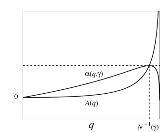
Figure 1: Typical graphs of ${\mathcal{A}}(q)$ and ${\mathfrak{A}}(q,\gamma)$ from (22) and (27) as functions of $q$. The graphs intersect each other, and ${\mathfrak{A}}(q,\gamma)$ attains its maximum, at $q={\mathcal{N}}^{-1}(\gamma)$. The maximum value ${\mathcal{A}}({\mathcal{N}}^{-1}(\gamma))$ is the minimum anisotropy of the input disturbance required to achieve the level $\gamma$ for the RMS gain of the system in (20). The mutual position of the graphs for $q\neq{\mathcal{N}}^{-1}(\gamma)$ is qualitatively described by (28).

the inequality ${|\!|\!|}F{|\!|\!|}_{a}\leqslant\gamma$ is equivalent to ${\mathcal{A}}({\mathcal{N}}^{-1}(\gamma))\geqslant a$. On the other hand, (29) implies that ${\mathcal{A}}({\mathcal{N}}^{-1}(\gamma))\geqslant a$ is equivalent to the existence of $q\in[0,\|F\|_{\infty}^{-2})$ such that ${\mathfrak{A}}(q,\gamma)\geqslant a$. Therefore,

$${\mathfrak{A}}(q,\gamma)\geqslant a\ {\rm for\ some}\ q\ \Longleftrightarrow\ {|\!|\!|}F{|\!|\!|}_{a}\leqslant\gamma.$$ (30)

Now, to prove (29), we differentiate the function ${\mathfrak{A}}$ from (27) in its first argument:

$${\rm\partial}_{q}{\mathfrak{A}}(q,\gamma)= \frac{1}{2}{\rm\partial}_{q}\ln\det(I_{\ell}-q\Lambda)+\frac{\ell\gamma^{2}}{2(1-q\gamma^{2})}$$

$$= -\frac{1}{2}{\rm Tr}(\Lambda{\mathcal{S}}(q))+\frac{\ell\gamma^{2}}{2(1-q\gamma^{2})}$$

$$-\frac{\ell{\mathcal{N}}(q)^{2}}{2(1-q{\mathcal{N}}(q)^{2})}+\frac{\ell\gamma^{2}}{2(1-q\gamma^{2})}$$

$$= \frac{\ell(\gamma^{2}-{\mathcal{N}}(q)^{2})}{2(1-q\gamma^{2})(1-q{\mathcal{N}}(q)^{2})},$$ (31)

where ${\rm\partial}_{q}(\cdot)$ is the partial derivative with respect to $q$, and use is made of (21), (24), (25). From (31) and the strict monotonicity of ${\mathcal{N}}$, it follows that ${\rm\partial}_{q}{\mathfrak{A}}(q,\gamma)$ is positive for $q<{\mathcal{N}}^{-1}(\gamma)$ and negative for $q>{\mathcal{N}}^{-1}(\gamma)$, thereby establishing (29).

We will now express the condition ${\mathfrak{A}}(q,\gamma)\geqslant a$ on the function (27) in terms of the state-space dynamics of the system (1)–(2) which has not been used yet. Recall that, for any conformable matrices $M$ and $U$, the spectra of $MU$ and $UM$ can differ from each other only by zeros (Horn & Johnson, 2007, Theorem 1.3.20 on p. 53). Hence, if we change the order in which $F_{0:N}^{{\rm T}}$ and $F_{0:N}$ are multiplied in the definition of the matrix $\Lambda$ in (19), then it follows that the spectrum of $I_{\ell}-q\Lambda$ differs from that of $I_{r(N+1)}-qF_{0:N}F_{0:N}^{{\rm T}}$ only by ones, and so

$$\det(I_{\ell}-q\Lambda)=\det(I_{r(N+1)}-qF_{0:N}F_{0:N}^{{\rm T}}).$$ (32)

Now, the latter matrix can be factorized for any $q<\|F\|_{\infty}^{-2}$ as

$$I_{r(N+1)}-qF_{0:N}F_{0:N}^{{\rm T}}=H_{0:N}H_{0:N}^{{\rm T}},$$ (33)

where the matrix $H_{0:N}$ represents an LDTV system $H$, whose input and output are both $r$-dimensional, on the time interval $[0,N]$. The factorization (33) is equivalent to that an ancillary system

$$\Psi:=\begin{bmatrix}\sqrt{q}F&H\end{bmatrix},$$ (34)

with an $(m+r)$-dimensional input and $r$-dimensional output, is outer on the time interval $[0,N]$, that is, $\Psi_{0:N}\Psi_{0:N}^{{\rm T}}=I_{r(N+1)}$. This property means that $\Psi$ transforms an $(m+r)$-dimensional Gaussian white noise sequence (with zero mean and identity covariance matrix) at the input into an $r$-dimensional sequence with the same properties at the output. The system $H$ can be found in the form

$$H=\left[\begin{array}[]{c|c}A_{\bullet}&M_{\bullet}\sqrt{S_{\bullet}}\\ \hline\cr C_{\bullet}&\sqrt{S_{\bullet}}\end{array}\right],$$ (35)

where the matrices $S_{0},\ldots,S_{N}$ are all positive definite, so that, in view of (3), the state-space realization of $\Psi$ in (34) is

$$\Psi=\left[\begin{array}[]{c|cc}A_{\bullet}&\sqrt{q}B_{\bullet}&M_{\bullet}\sqrt{S_{\bullet}}\\ \hline\cr C_{\bullet}&\sqrt{q}D_{\bullet}&\sqrt{S_{\bullet}}\end{array}\right].$$ (36)

Application of the state-space criterion of outerness from Appendix to (36) yields the Riccati equation (14)–(16), where $R_{0},\ldots,R_{N}$ are the controllability gramians of the system $\Psi$. Since (35) implies that $H_{0:N}$ is a block lower triangular matrix , that is,

$$H_{0:N}=\begin{bmatrix}\sqrt{S_{0}}&&0\\ &\ddots\\ *&&\sqrt{S_{N}}\end{bmatrix},$$

with the blocks $\sqrt{S_{0}},\ldots,\sqrt{S_{N}}$ over the main diagonal, then (32) and (33) yield

$$\det(I_{\ell}-q\Lambda)=(\det H_{0:N})^{2}=\prod_{k=0}^{N}\det S_{k}.$$

By substituting this representation into (27), it follows that the inequality ${\mathfrak{A}}(q,\gamma)\geqslant a$ in (30) is equivalent to (17).

6 Infinite anisotropy limit

If the anisotropy level increases unboundedly, $a\to+\infty$, then the localization (18), which follows from the inequality (17), yields $q\to\gamma^{-2}$. In this case, the Riccati equation (14)–(16) takes the form

$$R_{k+1} = A_{k}R_{k}A_{k}^{{\rm T}}+\gamma^{-2}B_{k}B_{k}^{{\rm T}}+M_{k}S_{k}M_{k}^{{\rm T}},$$ (37)

$$M_{k} = -(A_{k}R_{k}C_{k}^{{\rm T}}+\gamma^{-2}B_{k}D_{k}^{{\rm T}})S_{k}^{-1},$$ (38)

$$S_{k} = I_{r}-C_{k}R_{k}C_{k}^{{\rm T}}-\gamma^{-2}D_{k}D_{k}^{{\rm T}},$$ (39)

well-known in the context of ${\mathcal{H}}_{\infty}$-suboptimal controllers. This is closely related to the convergence $\lim_{a\to+\infty}{|\!|\!|}F{|\!|\!|}_{a}=\|F\|_{\infty}$ in (13), whereby the inequality ${|\!|\!|}F{|\!|\!|}_{a}\leqslant\gamma$ “approaches” $\|F\|_{\infty}\leqslant\gamma$ for large values of $a$. Therefore, in the limit, as $a\to+\infty$, Theorem 2 reduces to the Bounded Real Lemma, which establishes the equivalence between the inequality $\|F\|_{\infty}<\gamma$ and the positive definiteness of the matrices $S_{0},\ldots,S_{N}$ associated with (37)–(39).

7 Conclusion

We have considered a class of finite-dimensional linear discrete time varying systems on a bounded time interval subjected to input disturbances with an unknown probability law.

The statistical uncertainty has been quantified using the concept of anisotropy as an entropy theoretic measure of deviation of the actual noise distribution from nominal Gaussian white noise distributions with scalar covariance matrices.

The associated robust performance index, describing the worst-case disturbance attenuation capabilities of the system, is the $a$-anisotropic norm defined as the largest root mean square gain of the system with respect to random noises whose anisotropy is bounded by a given nonnegative parameter $a$.

We have established a state-space criterion for the $a$-anisotropic norm not exceeding a given threshold value. The Anisotropic Norm Bounded Real Lemma (ANBRL) is organised as an inequality on the determinants of matrices associated with a forward difference Riccati equation.

Apart from substantially simplifying the previously developed procedure of anisotropy-based robust performance analysis, which is now amenable to a recursive implementation, ANBRL includes the Bounded Real Lemma of the ${\mathcal{H}}_{\infty}$-control theory as a limiting case, thus extending it to the statistically uncertain stochastic setting with time varying dynamics.

*

Appendix A . State-space criterion of outerness

In this section, we assume that the output dimension of the system $F$ in (3) does not exceed the input dimension: $r\leqslant m$. Such a system is said to be outer on the time interval $[0,N]$ if $F_{0:N}F_{0:N}^{{\rm T}}=I_{r(N+1)}$. This is equivalent to the preservation of the property of being a Gaussian white noise sequence (with zero mean and identity covariance matrix) for signals passing through the system. The state-space criterion of outerness, given below for completeness of exposition, is similar to that in the time invariant case (Gu et al. (1989)) and utilizes the controllability and observability gramians

$$P_{j}:=\sum_{k=0}^{j-1}\Phi_{j,k+1}B_{k}B_{k}^{{\rm T}}\Phi_{j,k+1}^{{\rm T}},\quad Q_{k}:=\sum_{j=k}^{N}\Phi_{jk}^{{\rm T}}C_{j}^{{\rm T}}C_{j}\Phi_{jk},$$ (40)

where $\Phi_{jk}$ is the state transition matrix (5). The gramians satisfy the difference Lyapunov equations

$$P_{j+1}=A_{j}P_{j}A_{j}^{{\rm T}}+B_{j}B_{j}^{{\rm T}},\qquad Q_{k}=A_{k}^{{\rm T}}Q_{k+1}A_{k}+C_{k}^{{\rm T}}C_{k}$$

with initial condition $P_{0}=0$ and terminal condition $Q_{N+1}=0$.

Lemma 3

The LDTV system $F$ with the state-space realization (3) is outer on the time interval $[0,N]$ if and only if for every $k=0,\ldots,N$,

$$C_{k}P_{k}C_{k}^{{\rm T}}+D_{k}D_{k}^{{\rm T}}=I_{r},\qquad Q_{k+1}(A_{k}P_{k}C_{k}^{{\rm T}}+B_{k}D_{k}^{{\rm T}})=0.$$ (41)

Let the input $W$ to the system $F$ be an $m$-dimensional Gaussian white noise sequence with zero mean and identity covariance matrix. Then, in view of (2), the output $Z$ is also a zero mean Gaussian random sequence with

$${\bf cov}(z_{k})=C_{k}P_{k}C_{k}^{{\rm T}}+D_{k}D_{k}^{{\rm T}},$$ (42)

since $x_{k}$ and $w_{k}$ are independent, with ${\bf cov}(x_{k})=P_{k}$ the $k$th controllability gramian from (40). Consider the cross-covariance of $z_{j}$ and $z_{k}$ for $j>k\geqslant 0$. By using the state transition matrix (5), it follows that

$$z_{j}=C_{j}(\Phi_{j,k+1}x_{k+1}+\sum_{s=k+1}^{j-1}\Phi_{j,s+1}B_{s}w_{s})+D_{j}w_{j}.$$

Therefore, since $w_{k+1},\ldots,w_{j}$ are independent of $x_{k}$ and $w_{k}$, then

$${\bf cov}(z_{j},z_{k}) =C_{j}\Phi_{j,k+1}{\bf cov}(x_{k+1},z_{k})$$

$$=C_{j}\Phi_{j,k+1}(A_{k}P_{k}C_{k}^{{\rm T}}+B_{k}D_{k}^{{\rm T}}).$$

Hence, by recalling the observability gramian from (40), it follows that

$$\sum_{j=k+1}^{N}\|{\bf cov}(z_{j},z_{k})\|_{2}^{2}=\|\sqrt{Q_{k+1}}(A_{k}P_{k}C_{k}^{{\rm T}}+B_{k}D_{k}^{{\rm T}})\|_{2}^{2}.$$ (43)

Now, the system $F$ is outer on the time interval $[0,N]$ if and only if ${\bf cov}(z_{j},z_{k})=\delta_{jk}I_{r}$ for all $N\geqslant j\geqslant k\geqslant 0$, with $\delta_{jk}$ the Kronecker delta. In view of (42) and (43), the outerness is equivalent to (41).

References

- Bernhard (1998) H.-P.Bernhard, A tight upper bound on the gain of linear and nonlinear predictors for stationary stochastic processes, IEEE Trans. Signal Process., vol. 46, no. 11, 1998, pp. 2909–2917.
- Charalambous & Rezaei (2007) C.D.Charalambous, and F.Rezaei, Stochastic uncertain systems subject to relative entropy constraints: induced norms and monotonicity properties of minimax games, IEEE Trans. Autom. Contr., vol. 52, no. 4, 2007, pp. 647–663.
- Cover & Thomas (2006) T.M.Cover, and J.A.Thomas, Elements of Information Theory, Wiley, Hoboken, New Jersey, 2006.
- Diamond et al. (2001) P.Diamond, I.G.Vladimirov A.P.Kurdyukov and A.V.Semyonov, Anisotropy-based performance analysis of linear discrete time invariant control systems, Int. J. Contr., vol. 74, no. 1, 2001, pp. 28–42.
- Doyle et al. (1989) J.Doyle, K.Glover, P.Khargonekar, and B.Francis, State-space solutions to standard and -control problems. IEEE Trans. Automat. Contr., vol. 34, 1989, pp. 831–848.
- Dupuis et al. (2000) P.Dupuis, M.R.James, and I.R. Petersen, Robust properties of risk-sensitive control, Math. Contr. Sign. Sys., vol. 13, 2000, pp. 318–332.
- Gu et al. (1989) D.-W.Gu, M.C.Tsai, S.D.O’Young, and I.Postletwaite, State-space formulae for discrete-time optimization, Int. J. Contr., vol. 49, 1989, pp. 1683–1723.
- Horn & Johnson (2007) R.A.Horn, and C.R.Johnson, Matrix Analysis, Cambridge University Press, New York, 2007.
- Iglesias & Mustafa (1993) P.Iglesias, and D.Mustafa, State-space solution of the discrete-time minimum entropy control problem via separation, IEEE Trans. Automat. Contr., vol. 38, 1993, pp. 1525–1530.
- Kurdyukov et al. (2010) A.P.Kurdyukov, E.A.Maximov, and M.M.Tchaikovsky, Anisotropy-based bounded real lemma, Proc. 19th Int. Symp. Math. Theor. Networks Syst., Budapest, Hungary, July 5-9, 2010, pp. 2391–2397.
- Kurdyukov & Vladimirov (2008) A.P.Kurdyukov, and I.G.Vladimirov, Propagation of mean anisotropy of signals in flter connections, Proc. 17th World Congress IFAC, Seoul, Korea, July 6-11, 2008, pp. 6313–6318.
- Kwakernaak & Sivan (1972) H.Kwakernaak, and R.Sivan, Linear Optimal Control Systems, Wiley-Interscience, New York, 1972.
- Petersen et al. (2000) I.R.Petersen, M.R.James, and P.Dupuis, Minimax optimal control of stochastic uncertain systems with relative entropy constraints, IEEE Trans. Automat. Contr., vol. 45, no. 3, 2000, pp. 398–412.
- Petersen (2006) I.R.Petersen, Minimax LQG control, Int. J. Appl. Math. Comput. Sci., vol. 16, no. 3, 2006, pp. 309–323.
- Semyonov et al. (1994) A.V.Semyonov, I.G.Vladimirov, and A.P.Kurdyukov, Stochastic approach to -optimization, Proc. 33rd CDC, Florida, USA, December 14-16, vol. 3, 1994, pp. 2249–2250.
- Ugrinovskii & Petersen (2002) V.A.Ugrinovskii, and I.R. Petersen, Robust filtering of stochastic uncertain systems on an infinite time horizon, Int. J. Contr., vol. 75, no. 8, 2002, pp. 614–626.
- Vladimirov et al. (1995a) I.G.Vladimirov, A.P.Kurdjukov, and A.V.Semyonov, Anisotropy of signals and the entropy of linear stationary systems. Doklady Mathematics, vol. 51, no. 3, 1995, pp. 388–390.
- Vladimirov et al. (1995b) I.G.Vladimirov, A.P.Kurdjukov, and A.V.Semyonov, The stochastic problem of -optimization, Dokl. Akad. Nauk., vol. 52, no. 1, 1995, pp. 155–157.
- Vladimirov et al. (1996a) I.G.Vladimirov, A.P.Kurdjukov, and A.V.Semyonov, On computing the anisotropic norm of linear discrete-time-invariant systems, Proc. 13th IFAC World Congress, San-Francisco, California, USA, June 30-July 5, 1996, vol. G, pp. 179–184.
- Vladimirov et al. (1996b) I.G.Vladimirov, A.P.Kurdjukov, and A.V.Semyonov, State-space solution to anisotropy-based stochastic -optimization problem, Proc. 13th IFAC World Congress, San-Francisco, California, USA, June 30-July 5, 1996, vol. H, pp. 427–432.
- Vladimirov et al. (1999) I.G.Vladimirov, A.P.Kurdjukov, and A.V.Semyonov, Asymptotics of the anisotropic norm of linear time-invariant systems, Automat. Remote Contr., vol. 60, no. 3, 1999, pp. 359–366.
- Vladimirov et al. (2006) I.G.Vladimirov, P.Diamond, and P.Kloeden, Anisotropy-based robust performance analysis of finite horizon linear discrete time varying systems, Automat. Remote Contr., vol. 67, no. 8, 2006, pp. 1265–1282.
*