Inferring Genome-Wide Interaction Networks Using the Phi-Mixing Coefficient, and Applications to Lung Cancer
Abstract
Constructing gene interaction networks (GINs) from high-throughput gene expression data is an important and challenging problem in systems biology. Existing algorithms produce networks that either have undirected and unweighted edges, or else are constrained to contain no cycles, both of which are biologically unrealistic. In the present paper we propose a new algorithm, based on a concept from probability theory known as the phi-mixing coefficient, that produces networks whose edges are weighted and directed, and are permitted to contain cycles. Because there is no “ground truth” for genome-wide networks on a human scale, we analyzed the outcomes of several experiments on lung cancer, and matched the predictions from the inferred networks with experimental results. Specifically, we inferred three networks (NSCLC, Neuro-endocrine NSCLC plus SCLC, and normal) from the gene expression measurements of 157 lung cancer and 59 normal cell lines; compared with the outcomes of siRNA screening of 19,000+ genes on 11 NSCLC cell lines; and analyzed data from a ChIP-Seq experiment to determine putative downstream targets of the lineage specific oncogenic transcription factor ASCL1. The inferred networks displayed a scale-free or power law behavior between the degree of a node and the number of nodes with that degree. There was a strong correlation between the degree of a gene in the inferred NSCLC network and its essentiality for the survival of the cells. The inferred downstream neighborhood genes of ASCL1 in the SCLC network were significantly enriched by ChIP-Seq determined putative target genes, while no such enrichment was found in the inferred NSCLC network.
1 Introduction
The behavior of cells is governed by complex interactions amongst genes and gene products. Diseases such as cancer have their origin in a departure of these interactions from their normal patterns. By comparing the interactions that are present in normal cells versus cancerous cells, or between cells manifesting different forms of cancer, it is possible to draw some conclusions about the triggers of cancer and/or potential therapeutic targets.
Interactions and regulatory mechanisms that prevail between genes can be studied a few genes at a time, under carefully controlled experimental conditions. These interactions can then be aggregated to construct larger networks. However, such an approach is subject to two potential pitfalls. First, even aggregations of multiple public and commercial databases rarely contain more than 10,000 genes, whereas the human genome contains around 22,000 genes. The main reason for this is that biologists tend to study genes that are “interesting,” with the result that “uninteresting” genes and their neighborhoods do not get explored. The second potential pitfall is that the interactions in the aggregated network may be present under widely different, and perhaps even contradictory, experimental conditions; thus aggregating all these interactions into a common network may not be justifiable.
To overcome these potential pitfalls, in recent years there has been interest in reverse-engineering whole-genome interaction networks from simultaneous measurements of the expression levels of all (or at least most) genes in many samples, under a common set of experimental conditions. Such a network can be referred to as “whole-genome context-dependent.” In such an approach, the expression level of each gene is viewed as a random variable, say through where is the total number of genes whose measurements are taken. Then one attempts to construct a network (or graph) consisting of nodes, one for each gene, such that an interaction between two nodes is represented as an edge in the network between the corresponding nodes.
In order to make the theory work, assumptions are imposed on the underlying network that do not always coincide with biological realism. Existing methods for reverse-engineering whole-genome networks fall into two broad categories, which might be termed “Bayesian” and ‘information-based.” In the Bayesian framework [1, 2, 3, 4, 5], it is assumed that the network consists of directed edges and is acyclic. In other words, if there exists a path from gene to gene , there cannot exist a path from gene back to gene . This contradicts the fact that “real” biological networks contain a myriad of feedback loops in order to achieve stasis. In information-based methods, of which ARACNE [6] and CLR [7] are among the best-known, one computes a quantity called the mutual information between pairs of genes, and then uses a mathematical relationship known as the data processing inequality (DPI) to determine which interactions are to be retained in the network [6, 8, 9]. This approach can be proven to recover the joint probability distribution of all random variables, under the very restrictive assumption that the joint probability distribution consists of only first order or second order terms. The main drawback of this approach is that mutual information is a symmetric measure of the dependence between two random variables. Therefore networks constructed using information-based methods are perforce undirected. When one of the genes is a known transcription factor, the lack of directionality of the edges is not an isssue. However, when the aim is to infer genome-wide interaction networks, the lack of directionality is a serious shortcoming. Some of the recently developed methods such as GENIE3 [10] and bLARS [11] and ANOVA [12] can infer directed weighted graphs. However, to date these methods have been tested only on small organisms such as E. coli or synthetic data sets, and have not been assessed in the context of human genome-wide GIN.
Our motivation in devising yet another method for inferring interaction networks was to address each of the issues raised above. The algorithm presented here makes use of a directionally sensitive measure of dependence between random variables, known as the phi-mixing coefficient; accordingly the algorithm is referred to as “phixer.” The networks produced by phixer contain edges that are both directed as well as weighted (between and ), thus providing information about both the direction and the strength of the interaction between genes.
The phixer algorithm was used to reverse-engineer several gene interaction networks (GINs) in the context of lung cancer. These networks encompassed (i) non-small cell lung cancer (NSCLC), (ii) small cell lung cancer (SCLC), (iii) both of the above, and (iv) normal lung cells. One of the major difficulties in validating an inferred genome-wide GIN is that there is no “ground truth” network against which it can be compared. Therefore we used phixer-generated GINs to predict biological outcomes from whole-genome scale data sets, and compared against the actual outcomes. There was excellent agreement between the two, as described below. Thus we believe that the phixer algorithm offers an attractive, state of the art algorithm for inferring genome-wide GINs.
2 Theoretical Details
2.1 Background
In order to infer an interaction network from whole-genome expression data, one of the most commonly used approaches is to view the expression level of each gene as a random variable, and the measurements of the gene expression levels as independent samples of that random variable. Let denote the number of genes and denote the number of samples. Then the data is assumed to consist of statistically independent samples of the joint random variable . There is no assumption that these random variables are independent; indeed, the objective of the exercise is to determine their interdependence.
Suppose is a finite set, say .111Actually we should write , because the elements of are just labels and do not correspond to integers. Suppose is a random variable assuming values in with associated probability distribution . Thus . Then the entropy of , or the entropy of the probability distribution , is defined by
Now suppose are finite sets, and that are random variables assuming values in and respectively. Let denote the joint distribution of . Thus is a probability distribution on the product set . Let denote the marginals of on and respectively. Thus has the probability distribution and has the distribution . With this notation, the mutual information between and is defined as
An alternate and equivalent expression for the mutual information is
Mutual information is always symmetric and nonnegative; that is, . Moreover, if and only if and are independent random variables.
Suppose are random variables assuming values in finite sets respectively. Then and are said to be conditionally independent given , denoted by , if for all , it is true that
It is easy to show that the above relationship also implies that, for all , it is true that
A very useful inequality, known as the “data processing inequality” or DPI for short, states that whenever the following inequality holds:
| (1) |
See [13, p. 34] for a detailed discussion.
One of the first papers to infer GINs using mutual information is [14]. In that paper, the authors compute the mutual information between every pair of genes, and introduce an undirected edge between nodes and if and only if the mutual information between the corresponding random variables and exceeds a minimum threshold. They refer to the resulting (undirected) graph as an “influence network.” Indeed, in their framework, the presence of an (undirected) edge between two nodes and makes no distinction between gene influencing gene or vice versa. Also, no distinction is made between direct and indirect influence. As a consequence, the influence networks produced by the method in [14] are extremely dense.
Algorithm for the Reconstruction of Accurate Cellular Networks (ARACNE) [8] builds upon [14] and produces networks that are not overly dense by pruning out large number of edges. Specifically, for each triplet , they compute all the three mutual informations , and . Since the exact probability distributions are not known and only samples are available, they use Gaussian kernel approximations for the various joint distributions. Then they identify the smallest amongst the three numbers and discard the corresponding edge. Thus if
then they discard the edge between nodes and . The justification for the pruning strategy is that if the joint distribution of all random variables has the form
| (2) |
then the algorithm produces the correct interaction graph. However, the assumption that the joint probability distribution has the above form is quite unrealistic. Furthermore, the pruning strategy used in this algorithm implies that the GIN generated will never contain a complete subgraph of three nodes. In other words, if there is an edge between nodes and , and between nodes and , then there cannot be an edge between nodes and . But biology is full of small local networks that contain three-node complete subgraphs. Therefore new methods are required to generate more biologically realistic interaction networks.
2.2 Phi-mixing Coefficient as a Measure of Dependence
The phixer algorithm is based on computing the so-called -mixing coefficient between two random variables. The -mixing coefficient was introduced in [15] as a measure of the asymptotic long-term independence of a stationary stochastic process, and was used to prove laws of large numbers for non-i.i.d. processes. The general definition [16, Definition 2.1] can be readily adapted to define a quantitative measure of the dependence between two random variables [17, page 3].
If and are random variables assuming values in possibly distinct finite222The assumption that both random variables are finite-valued is made purely for convenience in exposition. In the general case, the sets and would have to belong to the -algebras generated by the random variables and respectively, and the maximum would have to be replaced by the supremum. sets and respectively, the -mixing coefficient is defined as
| (3) |
Thus is the maximum difference between the conditional and unconditional probabilities of an event involving only , conditioned over an event involving only . It is well known that the -mixing coefficient has the following properties:
-
1.
.
-
2.
In general, . Thus the -mixing coefficient gives directional information.
-
3.
and are independent random variables if and only if .
-
4.
The -mixing coefficient is invariant under any one-to-one transformation of the data. Thus if are one-to-one and onto maps, then
While (3) is suitable for defining the quantity , it cannot be directly used to compute it. Direct application of (3) requires us to take the maximum over all subsets of and , and would thus require computations. A recent paper [18] provides a closed form formula for the computation of , which implies that can be calculated in polynomial time. Let denote the joint distribution of and written out as a matrix. In other words,
Let denote the marginal distributions of and respectively; thus
Define as the outer product of and ; thus
Then is a rank one matrix, and is the joint distribution that and would have if they were independent. Define by
| (4) |
Thus would be the zero matrix if and were independent. Define
to be the matrix norm of induced by the vector -norm. Finally, for a given vector , let denote an diagonal matrix with the elements of on the diagonal. With these definitions, the following result can be derived.
Theorem 2.1
[18, Theorem 6] Suppose are random variables over finite sets with joint distribution and marginals respectively. Then
| (5) |
where denotes the nonnegative part of a number.
Note that Theorem 2.1 requires a total of algebraic operations and comparisons; therefore can be calculated in polynomial time.
Another very relevant property of the -mixing coefficient is given next.
Theorem 2.2
[18, Theorem 9] Whenever , the following inequality holds:
| (6) |
2.3 The Phixer Algorithm
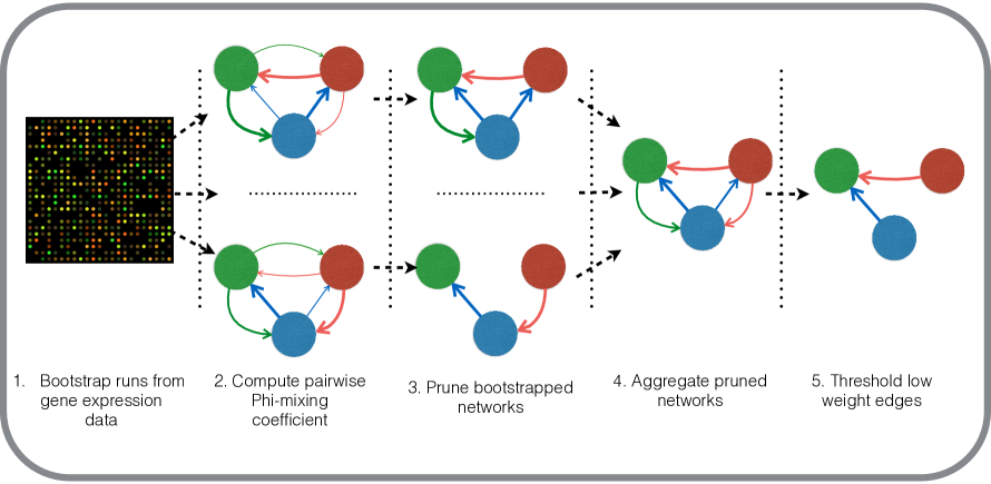
With the aid of the above properties, it is possible to design an algorithm for inferring GINs. The first step is called “pruning.” Start with a “complete” network where there is an edge from every node to every other node. Then, for each triplet of nodes, check whether Equation (6) is satisfied. If so, this means that the edge from node to node can be deleted, and the resulting network would still be consistent with the data. The order in which the triplets are checked does not affect the final network. The second step is called “thresholding,” and is a consequence of small sample sizes as are common in cancer data sets. In reality, we can compute only an approximation to the true number based on a finite number of cellular measurements. Consequently, even if the true value were to be zero, the computed value would not exactly be zero, though it would be small. Therefore all edges that remain after pruning should have their weights compared against a threshold, and those whose weight is smaller than this threshold should be seen as spurious and thus discarded. We have chosen a value of for the threshold, because if , then ignoring the possible dependence of on leads to a maximum error of % in computing various probabilities. One can play around with this threshold of , and the properties of the resulting networks do not vary very much. In the actual implementation, we employ bootstrapping, so as to ensure that the resulting network is very stable; see Figure 1.
Complete details of the implementation of the phixer algorithm are given in the supplementary material. A parallel implementation of the Phixer algorithm in C language is available at the web site https://github.com/nitinksingh/phixer.
2.4 Properties of the Phixer Generated GINs
The GINs produced by phixer algorithm have the following features:
-
1.
The GIN is invariant under any monotone transformation of the data. In other words, if are any monotonic functions, then the GIN produced by applying the algorithm to the original set will be exactly the same as the GIN produced by applying the algorithm to the transformed data set . This feature is useful as the post-processing of raw measurements often involves log transformation.
-
2.
The GIN has weighted, directional edges.
-
3.
Each edge in the GIN has a weight between and .
-
4.
The resulting GIN is permitted to contain cycles, and the edges are directional. That is, if and are two nodes in the GIN, then it is possible to have an edge from to but not from to , and it is also possible to have edges from to and from to , while the weights are the two edges could be different.
-
5.
The resulting GIN is strongly connected; that is, there is a directed path between every pair of nodes.
3 Results
3.1 Details of the Experiments Performed
Ideally the performance of a network inference algorithm should be assessed by comparing the predicted network with the actual network. Unfortunately, there is no “ground truth” for genome-wide networks on a human scale. Therefore we analyzed the outcomes of several experiments on lung cancer, and matched the predictions from the inferred networks with experimental results.
Specifically, we used the phixer algorithm to construct and characterize three networks based on the whole-genome gene-expression data (19,464 genes) of 157 lung cancer cell lines and one network from 59 normal lung tissue cell lines. The lung cancer cohort consisted of three distinct subtypes, namely: non-small cell lung cancer (NSCLC; 106 samples), small cell lung cancer (SCLC; 40 samples), and neuroendocrine non-small cell lung cancer (NE-NSCLC; 11 samples). Neuro-endocrine NSCLC is viewed as a separate subtype of NSCLC [19, 20, 21]. About 10% of the NSCLC cell lines show neuroendocrine morphological features that are characteristic of the SCLC subtype. These NE-NSCLC cell lines do in fact show a distinct gene-expression pattern compared to the rest of the NSCLC cell lines [21]. However, it is not possible to infer a network based on just 11 samples. Since NE-NSCLC appears to be closer to SCLC than NSCLC, we grouped the 11 NE-NSCLC cell lines with the 40 SCLC cell lines, to generate a total of 51 samples, which is nevertheless referred to as the SCLC cohort. The remainder of the 106 NSCLC cell lines are called the NSCLC cohort. The normal cell line cohort (59 samples) consists of both human bronchial epithelial cell (HBEC) and human small airway epithelial cells (HSAEC) cell lines.
These inferred networks were analyzed to see whether they exhibit scale-free or power law behavior. Next, these networks were used to predict the essentiality of each of the 19,000+ genes to the survival of a cancerous cell; the predictions were compared with the outcomes of siRNA screening of 19,000+ genes on 11 NSCLC cell lines. Finally, the immediate ancestors and successors of the lineage specific oncogenic transcription factor ASCL1 were determined from the inferred networks for SCLC and NSCLC cell lines. These were compared with the outcome of a ChIP-Seq experiment to determine putative downstream targets of ASCL1.
3.2 Phixer Generates Sparse and Scale Free Networks
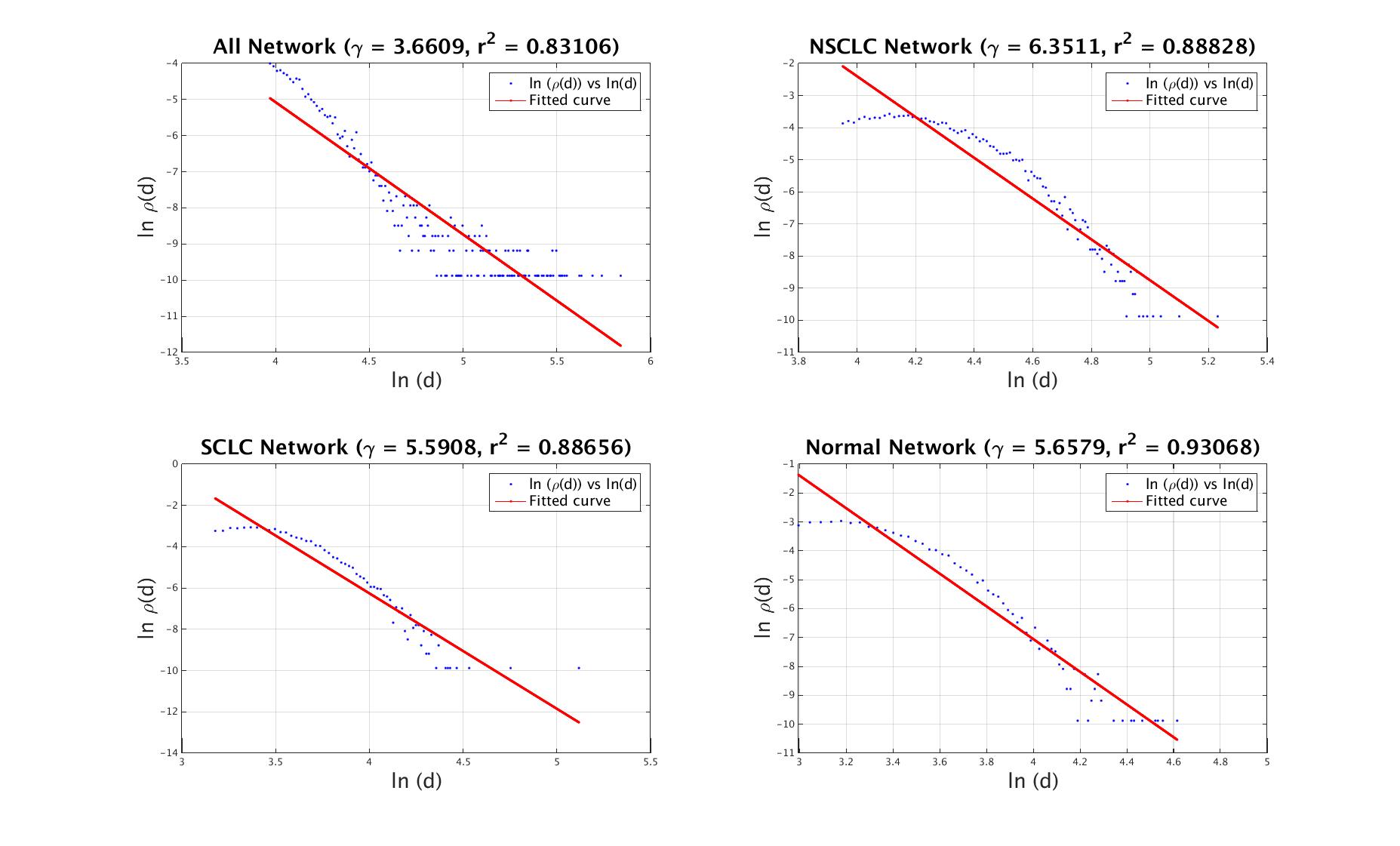
It is widely believed that real biological networks consist of a few “master regulators,” each of which controls hundreds of other genes, while the non-regulators have relatively few connections between themselves [22, 23]. The phixer-generated networks were analyzed on the basis of two parameters, namely degree distribution and the clustering coefficient, to determine how well they conform to this popular notion. Precise definitions of these two concepts are given in the Supplementary Material. But roughly speaking, the degree distribution measures the extent to which the network under study differs from a “random” network. In addition, we also examined whether the degree distributions in various phixer-generated networks display “scale-free” or “power law behavior,” whereby the number of nodes having a particular degree drops off as a power of the degree itself; in other words, on a log-log scale the plot looks linear. As shown in Figure 2, all four of the networks demonstrate a power law behavior. The clustering coefficient, as the name suggests, measures the tendency of nodes to cluster together. As shown in Figure 2, all four of the networks demonstrate small clustering coefficients.
3.3 Gene Connectivity versus its Essentiality
In this part of the study, we explored whether there is a relationship between the degree of a gene in the phixer-generated GIN and its essentiality for cell survival. It has been suggested that differentially expressed [24] or often mutated [25] genes in cancer have a higher degree in protein-protein interaction (PPI) networks. The advantage of PPI networks is that the edges correspond to regulatory relationships that have been experimentally validated. However, PPI networks have an element of a “self-fulfilling prophecy” in the sense that “interesting” genes are studied far more than “uninteresting” genes, with the result that “interesting genes” have more proven interactions. In short, one finds what one is looking for, a classic instance of finder’s bias. In contrast, the phixer algorithm “treats all genes equally” while generating the GIN. Therefore, if a gene degree in the phixer-generated GIN is substantially higher than that of another gene, this is a consequence of the data and not finder’s bias.
Specifically, we investigated whether there is a relationship between the degree of a gene in the phixer-generated network, and its essentiality for cell survival. The natural hypothesis is that higher degree genes are more essential to the cell than lower degree genes. To test this hypothesis, a subset of 11 NSCLC cell lines from the 106 samples used to infer the NSCLC network were subjected to genome-wide siRNA screening with two different siRNA libraries: Ambion and Dharmacon, resulting a set of 22 siRNA screening measurements. There were 18,534 common genes between the genome wide siRNA screening and the gene-expression measurements. The siRNA screening assay quantifies the intra-cellular ATP concentration for as a measure of the consequence of each gene depletion event on cell survival. The raw ATP concentration values were converted to -scores by subtracting the mean and dividing by the standard deviation. The resulting -scores are also referred to as the lethality scores. A higher (i.e., more positive or less negative) -score for a gene implies that the gene has relatively low effect on cell survival. On the other hand, a lower (more negative) -score implies that the gene is essential for cell survival. Therefore, as per the hypothesis, one would expect a negative correlation between the lethality score and the total degree of a gene. The significance of the resulting correlation is quantified against the null hypothesis that there is no negative correlation between the degree and lethality score. Therefore, the -values of the significance are calculated against the one-sided permutation distributions.
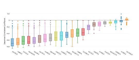
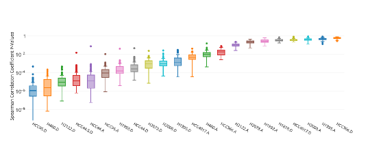
The degree of a gene in the GIN is indicative of its centrality in the network only at a coarse level, and not at a very fine grain level. To illustrate, a gene whose node degree is 400 is certainly more central than one whose node degree is 100; but it cannot be said to be more central than one whose node degree is 390. Therefore some amount of grouping genes by their degrees is warranted. To study the relation at a coarse level, we sorted the genes by their total degree and then aggregated them into groups consisting of genes each, where is varied from . Note that the case corresponds to computing the correlation between lethality of an individual gene and its total degree, without any grouping of genes. Now the correlation coefficient between the average leathality score and the average degree of these groups was computed. This kind of aggregate analysis was performed to study the robustness of the correlation over a wide range of group sizes. Figure 4 summarizes these results showing that 14 out of 22 cell-line screens have a statically significant (-value ) correlation. Evidently, for these 14 cell-lines, the negative correlation is robust to variations in the group size, with only a small number of outliers.
3.4 Phixer Infers Context-Specific Networks Accurately
3.4.1 Neighborhood of ASCL1 in the Inferred GIN is Enriched for ChIP Target Genes
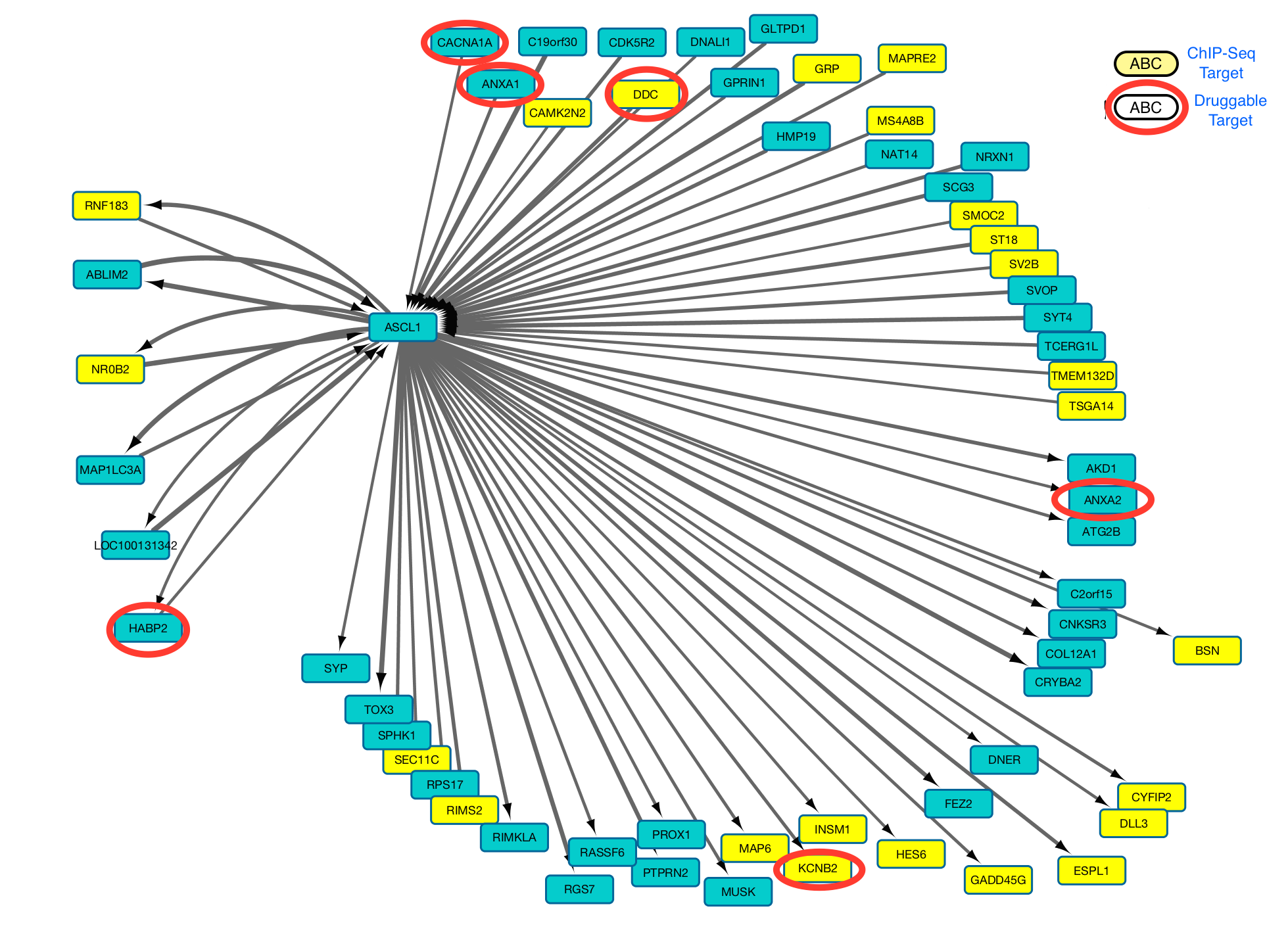
The predictive ability of the phixer algorithm was assessed by comparing the immediate neighborhood of the transcription factor achaete-scute homolog 1 (ASCL1) in the phixer-produced GIN with its putative targets obtained via an orthogonal ChIP-Seq experiment. The lineage specific transcription factor ASCL1 is required for the differentiation of pulmonary cells [26], and the initiation and survival of SCLC cells are dependent on its expression [27]. Further, it has been recently reported that ASCL1 is a lineage specific oncogene that is also required for the survival of NE-NSCLC cells [21]. A ChIP-Seq experiment was performed on two ASCL1(+) SCLC cell lines (NCI-H889 and NCI-H2107), while another two ASCL1(-) cell lines (NCI-H524 and NCI-H526) were used as controls. In the ChIP-Seq experiment, high quality peaks were analyzed for their functional association with the cis-regulatory regions with GREAT [28] yielding a set of potential ASCL1 targets. This gene set was further refined by filtering out genes whose expression in ASCL1(+) cell lines was less than 1.5 times that in the control. This resulted in a set of 226 putative ASCL1 target genes that were used for the validation of the phixer generated networks. In the inferred networks, any gene that has a direct edge from the ASCL1 is treated as its direct target. Note that the putative targets generated from ChIP-Seq studies represent direct transcriptional binding, while edges in the GIN represent “informational” interactions that may or may not correspond to “regulatory” binding.
The set of genes in the GIN that were downstream of ASCL1 was analyzed for enrichment of the ChIP-Seq generated putative target genes. The null hypothesis was that the downstream genes in the GIN were simply generated at random; therefore the -value was computed using the hypergeometric distribution. In the SCLC network based on 51 samples, out of 37 downstream neighbors of ASCL1 in the phixer-generated GIN, 6 were in the list of 226 ChIP-Seq genes, out of 19,464 genes in the network. The associated -value of this happening by chance is . In the network based on all 157 lung cancer samples, out of 119 downstream neighbors of ASCL in the phxer-generated GIN, 31 were from the ChIP-Seq list, for a -value of . In contrast, in the network based only on 106 NSCLC samples, out of the 27 downstream neighbors of ASCL1 in the phixer-generated GIN, only 1 was from the ChIP-Seq target list, for a -value of . This is consistent with the known fact that ASCL1 has a significant role only in SCLC (and its near-cousin, neuro-endocrine NSCLC), but not in NSCLC. Thus it would have been surprising had the neighborhood of ASCL1 been enriched with ChIP-Seq genes also in the NSCLC network. Figure 6 (a) illustrates the neighborhood of ASCL1 in the all lung cancer network.
3.4.2 ASCL1 Enrichment Results are Robust
As briefly mentioned in the introduction, phixer-generated networks are aggregated over many bootstrap runs and then finally undergo a thresholding step during which low weight edges are deleted. When two genes do not interact in reality, the theoretical phi-mixing coefficient should be zero. However, when the coefficient is estimated on the basis of a finite number of samples, the computed coefficient may not exactly equal zero, but will be small. Therefore, any edge whose computed mixing coefficient is smaller than can be deleted on the basis that the nonzero weight is an artifact of the small sample size. In the various networks, it is observed that a threshold higher than causes the network to become disconnected. The threshold value () is a user-defined parameter, and its actual value is determined from the distribution of the edge weights of the network; see SM Figure 1. The second parameter of the phixer algorithm is the number of bootstrap runs.
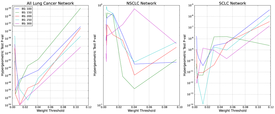
To study the effect of parameters on the ASCL1 enrichments, the number of bootstrap runs was varied from 100 to 300 in a step size of 50, while the threshold value was varied from 0 to , and the enrichment -values are computed. Figure 3(b) shows that the ASCL1 targets are enriched in all lung cancer network (-value ) and SCLC network (-value ) network, but not in the NSCLC network (-value ) for the range of parameter values studied. Applying a threshold higher than may cause these networks to become disconnected, and is hence not recommended. Figure 6 (b) also shows that the ASCL1 enrichment results are qualitatively the same for varying numbers of bootstrap runs. Since the run time of the algorithm scales linearly with the number of bootstrap runs, it is suggested to run the phixer algorithm only for 100 bootstrap runs. Together these results establish that the ASCL1 enrichment results are robust to the variation in phixer parameter values.
3.4.3 Phixer Compares Favorably with ARACNE
Algorithm for the Reconstruction of Accurate Cellular Networks (ARACNE) [8] is a widely used GIN inference algorithm that builds upon previous methods [14, 7] based on computing the mutual information between genes. The precursor to ARACNE is the influence network [14], which is an undirected graph consisting of edges between nodes and whenever the mutual information between genes and exceeds a user-defined threshold. Influence networks are extremely dense because they do not distinguish between direct and indirect influence. In ARACNE, one begins with the influence network, and then “prunes” it using the data processing inequality [13]. In this manner, ARACNE prunes an edge unless its presence is necessary to explain the data at hand. This algorithm has been validated in the context of human B-cells [6]. The main shortcoming of ARACNE, and other methods such as CLR that use mutual information as a criterion, is that the resulting network is always undirected, because the mutual information between two random variables is a symmetric quantity. Nevertheless, at present ARACNE is perhaps the most widely used algorithm for constructing mammalian GINs at a genome-wide scale.
The open source Linux version of the ARACNE software was downloaded from the official webpage333http://wiki.c2b2.columbia.edu/califanolab/index.php/Software/ARACNE and used for all the computations below. We generated all three lung cancer networks with the ARACNE algorithm with the default options with the exception of enabling the DPI (, default is 1 i.e., no DPI) and running for 100 bootstraps (, default is 1 to save time). The enrichment of the ASCL1 neighborhood in the ARACNE-generated network for the 226 ChIP-Seq putative targets was computed using the hypergeometric distribution, as earlier. In the SCLC network generated using 51 samples, 2 out of 16 neighbors were ChIP-Seq, for a -value of . In the all lung cancer network based on 157 samples, 6 out of 13 neighbors were ChIP-seq, for a -value of . In the NSCLC network based on 106 NSCLC samples, none of the 40 neighbors was a ChIP-Seq target, for a -value of 1. Note that since the ARACNE networks are undirected the ASCL1 targets consist both upstream and downstream targets. Recall that the corresponding -values for the phixer networks were (6 out of 37), (31 out of 119) and (1 out of 27), if only genes that are downstream of ASCL1 in the GIN are used to compute the -value. To make a like-to-like comparison with ARACNE, which does not provide any directional information of the interactions, we recomputed the -values using both upstream as well as downstream genes. The resulting -values were (6 out of 47), (46 out of 164) and (1 out of 54) for the SCLC, all lung cancer and NSCLC networks respectively. This shows that phixer provides a more accurate and context specific neighborhood for ASCL1 compared to the ARACNE algorithm. We observe that the ASCL1 neighborhood predicted by the ARACNE network contains far fewer genes than one would expect for an oncogene that is critical to the initiation and survival of neuroendocrine lineage lung cancers. In contrast, the number of downstream genes of ASCL1 in the phixer-generated GIN, using the suggested threshold of 0.1 for the weight, is quite reasonable for an oncogene. Moreover, the phixer algorithm provides a threshold parameter to control the sparsity of the resulting network.
4 Discussion
As gene interaction networks (GINs) can shed light on fundamental biological processes and disease mechanisms, systematic construction of GINs from high-throughput gene expression data is one of the important problems in systems biology. In this paper, we have presented a new algorithm, named phixer, to infer GINs from gene expression data. In contrast with existing algorithms, the phixer algorithm generates a network whose edges are directed and weighted, and is also permitted to contain cycles. This is in contrast to information-based methods which lead to undirected graphs, and Bayesian methods which lead to acyclic graphs. The proposed method was utilized to construct and contrast three lung cancer networks and one network from normal tissue samples. An analysis of these networks revealed that they display a power law behavior (also known as “scale-free” behavior) and clustering properties; this matches widely-held expectations that real world biological networks have these properties. It is widely believed that “hub” genes, that is, genes that interact with many other genes, are more essential to cell survival than genes with fewer interactions. This hypothesis was tested on 11 lung cancer cell lines using two different reagents to perform siRNA knockdown experiments. The lethality score of each gene on each cell line was correlated with its node degree in the inferred GIN. In 14 out of 22 experiments, there was a statistically significant correlation. Finally, the putative target genes of the transcription factor ASCL1, as determined by a ChIP-seq experiment, were tested against the predicted upstream and downstream genes of ASCL1 in the inferred GIN. The neighborhood was enriched with the putative target genes with an extremely low -value. A comparison of phixer with widely used GIN construction algorithm ARACNE shows that the ASCL1 neighborhood is enriched with ChIP-Seq targets to a far higher extent in the network constructed using the phixer algorithm, compared to the network constructed using ARACNE. In addition, the run time of phixer is about half that of ARANCE (see Methods section).
The ability to infer context specific GINs may prove to be a valuable tool to investigate biological processes that have a clinical potential. First, the observation that there is a significant correlation between the degree of a gene in the reverse-engineered GIN and its lethality score can be of clinical value, by identifying genes that can be suppressed to reduce cancer cell proliferation, whether or not the genes have a known role in the onset or progression of the disease. This relationship could potentially be exploited to seek genes whose activation (or inactivation) is lethal to tumor cells but relatively innocuous to the normal cells. Second, identifying druggable upstream regulators of an oncogene is valuable when the oncogene might not itself be directly druggable. Of course, any such hypotheses based on the inferred GIN must then be validated experimentally.
The performance of any network GIN inference method, including phixer, is governed by the number of available samples. Because the method requires the estimation of the dependence between two random variables, ideally the number of samples should in excess of 100. Also, it must be recognized that the edges in the network represent “informational” relationships that may not necessarily correspond to physical interaction or causation. Nevertheless, we believe that the context specific GINs inferred using the phixer algorithm will be useful to shed light on interesting biological hypotheses.
Acknowledgements
The authors thank Prof. John Minna, Prof. Jane Johnson, Dr. Alex Augustyn and Dr. Mark Borromeo for the gene-expression and ChIP-Seq data.
NS, MEA, SM and MV were supported by the National Science Foundation under ECCS Awards #1001643 and #1306630; the Cancer Prevention and Research Institute of Texas (CPRIT) under grants RP110595 and RP140517; the Jonsson Family Graduate Fellowships; and the Cecil H. and Ida Green Endowment at the University of Texas at Dallas. HSK was supported by the National R&D Program for Cancer Control, Ministry of Health & Welfare, Republic of Korea #1420100, and in part by the CPRIT training grant RP101496. MAW was supported by the Welch Foundation award I-1414, and NIH grants CA197717, and CA176284.
References
- [1] N. Friedman, M. Linial, I. Nachman, and D. Pe’er, “Using Bayesian networks to analyze expression data.” Journal of Computational Biology, vol. 7, no. 3-4, pp. 601–20, jan 2000. [Online]. Available: http://www.ncbi.nlm.nih.gov/pubmed/11108481
- [2] Y. Barash and N. Friedman, “Context-specific Bayesian clustering for gene expression data,” J. Comput. Biol., vol. 9(2), pp. 169–191, 2002.
- [3] N. Friedman, “Inferring cellular networks using probabilistic graphical models,” Science, vol. 303, pp. 799–805, 2004.
- [4] J. Yu, V. A. Smith, P. P. Wang, A. J. Hartemink, and E. D. Jarvis, “Advances to Bayesian network inference for generating causal networks from observational biological data.” Bioinformatics (Oxford, England), vol. 20, no. 18, pp. 3594–603, dec 2004.
- [5] D. Koller and N. Friedman, Probabilistic Graphical Models: Principles and Techniques. MIT Press, Cambridge, MA, 2009.
- [6] K. Basso, A. Margolin, G. Stolovitzky, U. Klein, R. Dalla-Favera, and A. Califano, “Reverse engineering of regulatory networks in human B cells.” Nature genetics, vol. 37, no. 4, pp. 382–390, 2005.
- [7] J. J. Faith, B. Hayete, J. T. Thaden, I. Mogno, J. Wierzbowski, G. Cottarel, S. Kasif, J. J. Collins, and T. S. Gardner, “Large-scale mapping and validation of Escherichia coli transcriptional regulation from a compendium of expression profiles.” PLoS Biology, vol. 5, no. 1, p. e8, jan 2007. [Online]. Available: http://www.pubmedcentral.nih.gov/articlerender.fcgi?artid=1764438–“&˝tool=pmcentrez–“&˝rendertype=abstract
- [8] A. Margolin, I. Nemenman, K. Basso, C. Wiggins, G. Stolovitzky, R. Dalla Favera, and A. Califano, “ARACNE: an algorithm for the reconstruction of gene regulatory networks in a mammalian cellular context.” in BMC Bioinformatics, vol. 7, jan 2006, pp. 1–15.
- [9] I. S. Jang, A. Margolin, and A. Califano, “hARACNe : improving the accuracy of regulatory model reverse engineering via higher-order data processing inequality tests,” Interface Focus, vol. 3, no. 4, pp. 1–11, 2013.
- [10] V. A. Huynh-Thu, A. Irrthum, L. Wehenkel, and P. Geurts, “Inferring regulatory networks from expression data using tree-based methods.” PloS One, vol. 5, no. 9, pp. 1–10, jan 2010.
- [11] N. Singh and M. Vidyasagar, “bLARS: An Algorithm to Infer Gene Regulatory Networks,” IEEE/ACM Transactions on Computational Biology and Bioinformatics, pp. 1–1, 2015. [Online]. Available: http://ieeexplore.ieee.org/articleDetails.jsp?arnumber=7138615
- [12] R. Küffner, T. Petri, P. Tavakkolkhah, L. Windhager, and R. Zimmer, “Inferring gene regulatory networks by ANOVA.” Bioinformatics (Oxford, England), vol. 28, no. 10, pp. 1376–82, may 2012.
- [13] T. M. Cover and J. A. Thomas, Elements of Information Theory. Wiley Interscience, New York, 2006.
- [14] A. J. Butte and I. S. Kohane, “Mutual information relevance networks: functional genomic clustering using pairwise entropy measurements.” in Pacific Symposium on Biocomputing, jan 2000, pp. 415–426. [Online]. Available: http://www.ncbi.nlm.nih.gov/pubmed/10902190
- [15] I. A. Ibragimov, “Some limit theorems for stationary processes,” Theory of Probability and its Applications, vol. 7, pp. 349–382, 1962.
- [16] M. Vidyasagar, Learning and Generalization: With Applications to Neural Networks and Control Systems. Springer-Verlag, London, 2003.
- [17] P. Doukhan, Mixing: Properties and Examples. Springer-Verlag, Heidelberg, 1994.
- [18] M. E. Ahsen and M. Vidyasagar, “Mixing Coefficients Between Discrete and Real Random Variables : Computation and Properties,” IEEE Transactions on Automatic Control, vol. 59, no. 1, pp. 34–47, 2014.
- [19] A. Bhattacharjee, W. G. Richards, J. Staunton, C. Li, S. Monti, P. Vasa, C. Ladd, J. Beheshti, R. Bueno, M. Gillette, M. Loda, G. Weber, E. J. Mark, E. S. Lander, W. Wong, B. E. Johnson, T. R. Golub, D. J. Sugarbaker, and M. Meyerson, “Classification of human lung carcinomas by mRNA expression profiling reveals distinct adenocarcinoma subclasses.” Proceedings of the National Academy of Sciences of the United States of America, vol. 98, no. 24, pp. 13 790–5, nov 2001.
- [20] M. H. Jones, C. Virtanen, D. Honjoh, T. Miyoshi, Y. Satoh, S. Okumura, K. Nakagawa, H. Nomura, and Y. Ishikawa, “Two prognostically significant subtypes of high-grade lung neuroendocrine tumours independent of small-cell and large-cell neuroendocrine carcinomas identified by gene expression profiles.” Lancet, vol. 363, no. 9411, pp. 775–81, mar 2004.
- [21] A. Augustyn, M. Borromeo, T. Wang, J. Fujimoto, C. Shao, P. D. Dospoy, V. Lee, C. Tan, J. P. Sullivan, J. E. Larsen, L. Girard, C. Behrens, I. I. Wistuba, Y. Xie, M. H. Cobb, A. F. Gazdar, J. E. Johnson, and J. D. Minna, “ASCL1 is a lineage oncogene providing therapeutic targets for high-grade neuroendocrine lung cancers.” Proceedings of the National Academy of Sciences of the United States of America, vol. 111, no. 41, pp. 14 788–93, oct 2014.
- [22] A. Barabási, “Emergence of Scaling in Random Networks,” Science, vol. 286, no. 5439, pp. 509–512, oct 1999. [Online]. Available: http://www.sciencemag.org/content/286/5439/509.abstract
- [23] M. E. J. Newman, “Random graphs as models of networks,” in Handbook of Graphs and Networks, S. B. Schuster and H. G., Eds. Wiley-VCH, Berlin, feb 2003, no. 1, pp. 35–68.
- [24] S. Wachi, K. Yoneda, and R. Wu, “Interactome-transcriptome analysis reveals the high centrality of genes differentially expressed in lung cancer tissues.” Bioinformatics (Oxford, England), vol. 21, no. 23, pp. 4205–8, dec 2005.
- [25] P. F. Jonsson and P. Bates, “Global topological features of cancer proteins in the human interactome.” Bioinformatics, vol. 22, no. 18, pp. 2291–2297, sep 2006.
- [26] M. Borges, R. I. Linnoila, H. J. van de Velde, H. Chen, B. D. Nelkin, M. Mabry, S. B. Baylin, and D. W. Ball, “An achaete-scute homologue essential for neuroendocrine differentiation in the lung.” Nature, vol. 386, no. 6627, pp. 852–5, apr 1997.
- [27] T. Jiang, B. J. Collins, N. Jin, D. N. Watkins, M. V. Brock, W. Matsui, B. D. Nelkin, and D. W. Ball, “Achaete-scute complex homologue 1 regulates tumor-initiating capacity in human small cell lung cancer.” Cancer research, vol. 69, no. 3, pp. 845–54, mar 2009.
- [28] C. Y. McLean, D. Bristor, M. Hiller, S. L. Clarke, B. T. Schaar, C. B. Lowe, A. M. Wenger, and G. Bejerano, “GREAT improves functional interpretation of cis-regulatory regions.” Nature biotechnology, vol. 28, no. 5, pp. 495–501, may 2010.