NLO QCD corrections to off-shell $\mathrm{t\bar{t}}$ production at hadron colliders

Abstract:

The production of top–antitop-quark pairs at hadron colliders is interesting both in its own right as signal process, but also as background to many searches for new physics. The corresponding predictions aim at the precision level of few per cent, rendering not only the inclusion of radiative corrections of the strong and electroweak interactions relevant, but also of off-shell and finite-width effects originating from the top-quark decays ${\mathrm{t}}\to{\mathrm{b}}{\mathrm{W}}\to{\mathrm{b}}+l^{+}\nu_{l}/q\bar{q}^{\prime}$. We report on a calculation for the full process ${\mathrm{p}}{\mathrm{p}}\to{\mathrm{W}}^{+}{\mathrm{W}}^{-}{\mathrm{b}}\bar{\mathrm{b}}\to{\nu_{\mathrm{e}}{\mathrm{e^{+}}}{\mathrm{\mu^{-}}}\bar{\nu}_{\mu}{\mathrm{b}}\bar{\mathrm{b}}}$ at next-to-leading order QCD and discuss the effects of the finite widths of the top quarks and of the W bosons for selected observables. Generically it turns out that finite-top-width effects are at the per-cent level whenever the top-quark resonances dominate, but those effects can reach tens of per cent in off-shell tails. Finite-W-width effects, on the other hand, are suppressed to less than $0.5\%$ whenever the top quarks can become resonant and only become sizeable in exceptional cases. One such case, however, is the invariant mass of a bottom quark and the corresponding charged lepton, which result from the same top-quark decay—an observable that is relevant for precision measurements of the top-quark mass.

1 Introduction

After about 17 years of its discovery, experimental studies of the top quark are still highly interesting, since the top quark is expected to serve as a key for understanding the fermionic mass hierarchy and to be potentially sensitive to physics beyond the Standard Model. Evidently, accurate measurements of top–antitop pairs carried out at the Tevatron and the LHC must be accompanied by precise calculations. A survey of LHC results on top-quark physics and corresponding theoretical predictions can be found in the recent review [1]. In this article we can only concentrate on the specific issue of off-shell and finite-width effects and the corresponding literature.

Since many years, ${\mathrm{t}}\bar{\mathrm{t}}$ production at hadron colliders is fully known at next-to-leading-order (NLO) within QCD and electroweak theory. Beyond fixed order, the resummation of logarithmically enhanced QCD corrections got more and more refined as well. Most recently, a major step was made towards a full prediction at next-to-next-to-leading-order QCD upon completing the quark–antiquark channel [2], which is dominating ${\mathrm{t}}{\mathrm{\bar{t}}}$ production at the Tevatron. Most predictions, however, are based on the approximation of stable (on-shell) top quarks, i.e. the top-quark decays, which proceed into pairs of W bosons and bottom quarks in the Standard Model, are ignored. A first important step towards a full NLO description of top-pair production and decay was made in Refs. [3, 4, 5], where top-quark decays were treated in a spin-correlated narrow-width approximation, i.e. the top quarks are still on shell, but spin correlations between production and decay are taken into account. Recently, first results at NLO QCD for the complete process of ${\mathrm{W}}^{+}{\mathrm{W}}^{-}{\mathrm{b}}\bar{\mathrm{b}}$ production, with intermediate off-shell top quarks and including leptonic W-boson decays have been obtained by two independent groups [6, 7, 8].

As long as resonant ${{\mathrm{t}}\bar{\mathrm{t}}}$ production dominates an observable, finite-width effects of the top quark are suppressed to the order of ${\cal O}(\Gamma_{{\mathrm{t}}}/m_{\mathrm{t}})\sim 1\%$. The finite-W-width effects even turn out to be suppressed to the level ${\cal O}(\Gamma_{{\mathrm{t}}}/m_{\mathrm{t}}\times\Gamma_{{\mathrm{W}}}/m_{{\mathrm{W}}})$ in inclusive observables [8]. However, in more exclusive measurements, such as precision $m_{\mathrm{t}}$ determinations, ${{\mathrm{t}}\bar{\mathrm{t}}}$ backgrounds to new physics that are suppressed by vetoing top resonances, or the ${{\mathrm{t}}\bar{\mathrm{t}}}$ background to ${\mathrm{H}}\to ll\nu\nu$ signals in presence of b-jet vetoes, the investigation of finite-top-width effects is even more important since their magnitude is not known a priori. A first systematic study of finite-top-width effects in exclusive observables [9], based on a comparison of our calculation against the narrow-top-width approximation of Ref. [4], indicates that finite-top-width corrections to phenomenologically important observables can range from a few per mille to tens of per cent. This also raises the issue of possible non-negligible effects resulting from the finite width of intermediate W bosons, which is addressed in detail in Ref. [8].

In this article we briefly discuss results from the off-shell calculation [6, 8] and compare them to the narrow-width approximation of Ref. [4], in order to work out the genuine finite-width effects of the top quark and the W boson.

2 Features of off-shell $\mathrm{t\bar{t}}$ production

The process ${\mathrm{p}}{\mathrm{p}}\to{\mathrm{W}}^{+}{\mathrm{W}}^{-}{\mathrm{b}}\bar{\mathrm{b}}+X\to{\nu_{\mathrm{e}}{\mathrm{e^{+}}}{\mathrm{\mu^{-}}}\bar{\nu}_{\mu}{\mathrm{b}}\bar{\mathrm{b}}}+X$ describes hadronic top-quark pair production with subsequent leptonic top-quark decays. The corresponding matrix elements comprise doubly-resonant contributions, where the ${\nu_{\mathrm{e}}{\mathrm{e^{+}}}{\mathrm{\mu^{-}}}\bar{\nu}_{\mu}{\mathrm{b}}\bar{\mathrm{b}}}$ final state results from the decay of a ${\mathrm{t}}\bar{\mathrm{t}}$ pair, as well as singly-resonant and non-resonant diagrams, i.e. contributions with only one or no top resonance. While diagrams with intermediate ${\mathrm{t}}\bar{\mathrm{t}}$ states always contain two W-boson resonances from the top-quark decays, the remaining background diagrams involve one or two resonant W bosons. Typical leading-order (LO) and NLO diagrams for partonic channels with different resonance structures are shown in Figure 1.

0.83

Figure 1: Typical partonic diagrams contributing to ${\mathrm{p}}{\mathrm{p}}\to{\mathrm{W}}^{+}{\mathrm{W}}^{-}{\mathrm{b}}\bar{\mathrm{b}}\to{\nu_{\mathrm{e}}{\mathrm{e^{+}}}{\mathrm{\mu^{-}}}\bar{\nu}_{\mu}{\mathrm{b}}\bar{\mathrm{b}}}$ at LO (first row), to the NLO virtual corrections (second row), and to the NLO real corrections (last row).

In the following we discuss results of our NLO QCD calculation [8] of the process ${\mathrm{p}}{\mathrm{p}}\to{\mathrm{W}}^{+}{\mathrm{W}}^{-}{\mathrm{b}}\bar{\mathrm{b}}+X\to{\nu_{\mathrm{e}}{\mathrm{e^{+}}}{\mathrm{\mu^{-}}}\bar{\nu}_{\mu}{\mathrm{b}}\bar{\mathrm{b}}}+X$ and of its earlier version [6]. At LO we fully take into account all diagrams with any number of intermediate top-quark and W-boson resonances, i.e. all off-shell effects are included. For the real-emission corrections we follow the same procedure. To regularize the resonances in a gauge-invariant way we employ the complex-mass scheme [10], where the decay widths $\Gamma_{i}$ ($i={\mathrm{t}},{\mathrm{W}}$) are incorporated into the definition of the (squared) masses, $\mu^{2}_{i}=m_{i}^{2}-{\mathrm{i}}m_{i}\Gamma_{i}$. All matrix elements are evaluated using the complex masses $\mu_{i}$, so that resonant and non-resonant contributions are uniformly described. In principle, it would be possible to proceed for the virtual NLO corrections in the same way (as it was done in Ref. [7]), but we decided to proceed somewhat differently. While we still take into account all diagrams with any number of on- or off-shell top quarks, we treat the W-boson resonances in the so-called double-pole approximation (DPA), where only the leading contribution in an expansion about the W resonances is kept. This procedure reduces the set of loop diagrams to the ones with two W resonances only and guarantees NLO accuracy in the vicinity of the two W-boson resonances, which includes all regions with one or two intermediate resonant top quarks. As discussed below, the finite-W-width (FwW) effects receive an additional suppression, rendering this approximation rather good. Another motivation for using the DPA resides in the possibility to include the electroweak NLO corrections without the necessity to deal with the irreducible $2\to 6$ particle reaction; the DPA effectively splits the full process into ${{\mathrm{W}}{\mathrm{W}}{\mathrm{b}}\bar{\mathrm{b}}}$ production of $2\to 4$ type with the subsequent W decays of $1\to 2$ type.

The rest of our NLO calculation follows the standard procedure of a diagrammatic calculation, as described in Refs. [6, 8] in more detail.

3 Numerical results on finite-top-width and finite-W-width effects

Generically, when a resonance is integrated over in an observable, finite-width effects are of the order of $\Gamma_{i}/m_{i}$. This is nicely seen for the finite-top-width (FtW) effects on integrated cross sections and distributions that are dominated by the double top-quark resonance. As discussed in Refs. [6, 7, 9, 8] in detail for the Tevatron and the LHC at various energies, the FtW effects on those observables are of the typical size of ${\cal O}(\Gamma_{{\mathrm{t}}}/m_{\mathrm{t}})\sim 1\%$.

The situation for FwW effects is different. Observables that are dominated by resonant ${\mathrm{t}}{\mathrm{\bar{t}}}$ production involve W resonances only through the top-quark decays, and effectively any correction to these decays manifests itself as correction to the respective top-quark branching ratio. However, since FwW effects are universal for all top decay channels, they cancel in the branching ratio. Thus, FwW effects come only in combination with FtW effects in observables dominated by ${\mathrm{t}}{\mathrm{\bar{t}}}$ production, resulting in an additional suppression of ${\cal O}(\Gamma_{{\mathrm{t}}}/m_{\mathrm{t}}\times\Gamma_{{\mathrm{W}}}/m_{{\mathrm{W}}})<0.5\%$. The numerical enhancement in the number $0.5\%$, which is read off from our numerical study [8], results from phase-space cuts that disturb the inclusiveness used in the power-counting argument.

In the following we exemplarily discuss FtW and FwW effects on two distributions of phenomenological interest where those effects do not receive the suppression described above. The FtW effects are quantified upon comparing the results from our off-shell calculation with the ones obtained in the (spin-correlated) narrow-top-width approximation (NtWA) of Ref. [4]. The FwW effects are estimated by the difference between the two versions [8] and [6] of our calculation with off-shell and on-shell W bosons, respectively, as described above. The shown results are taken from Refs. [9, 8], where all details on the underlying input and setup (which is not exactly the same in Refs. [9, 8]) can be found.

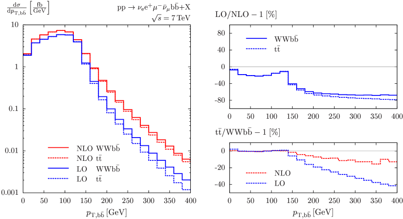
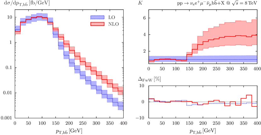
Figures 3 and 3 show the finite-width effects on the transverse-momentum distribution of the ${\mathrm{b}}{\mathrm{\bar{b}}}$ pair, which plays an important role in boosted-Higgs searches with a large ${{\mathrm{t}}\bar{\mathrm{t}}}$ background.

Figure 2: Transverse-momentum distribution of the ${\mathrm{b}}{\mathrm{\bar{b}}}$ pair for the LHC at $\sqrt{s}=7\,\mathrm{TeV}$, showing the absolute LO and NLO predictions (left), the relative NLO corrections (upper right), and the relative difference (lower right) between the NtWA (${\mathrm{t}}{\mathrm{\bar{t}}}$) and the off-shell calculation (${\mathrm{W}}{\mathrm{W}}{\mathrm{b}}{\mathrm{\bar{b}}}$). (Taken from Ref. [9].)

Figure 3: Transverse-momentum distribution of the ${\mathrm{b}}{\mathrm{\bar{b}}}$ pair for the LHC at $\sqrt{s}=8\,\mathrm{TeV}$ showing the absolute LO and NLO predictions with the bands illustrating the scale uncertainty (left), the NLO $K$ factor (upper right), and the finite-W-width effects (lower right). (Taken from Ref. [8].)

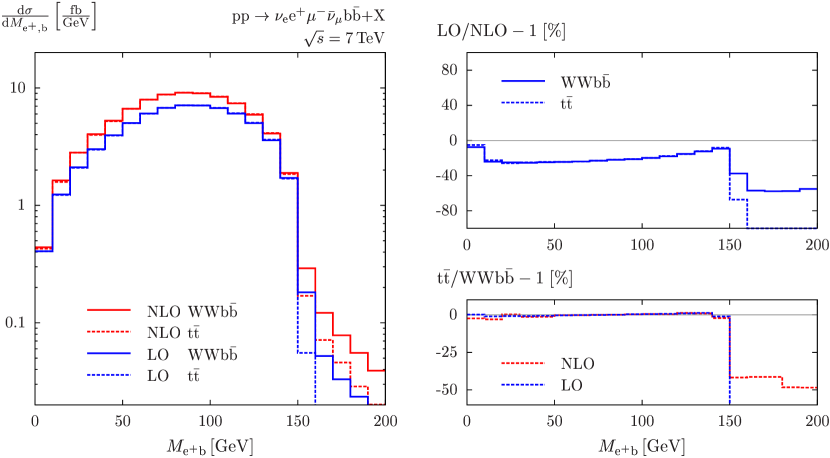
Figure 4: Invariant-mass distribution of positron–$\mathrm{b}$-jet system for the LHC at $\sqrt{s}=7\,\mathrm{TeV}$, showing the absolute LO and NLO predictions (left), the relative NLO corrections (upper right), and the relative difference (lower right) between the NtWA (${\mathrm{t}}{\mathrm{\bar{t}}}$) and the off-shell calculation (${\mathrm{W}}{\mathrm{W}}{\mathrm{b}}{\mathrm{\bar{b}}}$). (Taken from Ref. [9].)

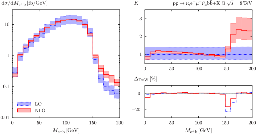
Figure 5: Invariant-mass distribution of positron–$\mathrm{b}$-jet system for the LHC at $\sqrt{s}=8\,\mathrm{TeV}$ showing the absolute LO and NLO predictions with the bands illustrating the scale uncertainty (left), the NLO $K$ factor (upper right), and the finite-W-width effects (lower right). (Taken from Ref. [8].)

The extraction of ${\mathrm{p}}{\mathrm{p}}\to{\mathrm{H}}(\to{\mathrm{b}}\bar{\mathrm{b}}){\mathrm{W}}$ signal at the LHC is based on the selection of boosted ${\mathrm{H}}\to{\mathrm{b}}\bar{\mathrm{b}}$ candidates with $p_{{\mathrm{T}},{\mathrm{b}}\bar{\mathrm{b}}}>200\,\,\mathrm{GeV}$, which permits to reduce ${{\mathrm{t}}\bar{\mathrm{t}}}$ contamination. The suppression of ${{\mathrm{t}}\bar{\mathrm{t}}}$ production is indeed particularly strong at $p_{{\mathrm{T}},{\mathrm{b}}\bar{\mathrm{b}}}\mathrel{\raisebox{-3.00003pt}{$\stackrel{{\scriptstyle\displaystyle>}}{{\sim}}$}}150\,\,\mathrm{GeV}$. This is due to the fact that, for resonant ${\mathrm{t}}{\mathrm{\bar{t}}}$ pairs, ${\mathrm{b}}$ quarks need to be boosted via the $p_{\mathrm{T}}$ of their parent (anti)top quarks in order to acquire $p_{{\mathrm{T}},{\mathrm{b}}}>(m_{\mathrm{t}}^{2}-m_{{\mathrm{W}}}^{2})/(2m_{\mathrm{t}})\simeq 65\,\,\mathrm{GeV}$, and a ${\mathrm{b}}\bar{\mathrm{b}}$ system with high $p_{\mathrm{T}}$ is kinematically strongly disfavoured at LO, since top and antitop quarks have opposite transverse momenta. The NLO corrections undergo less stringent kinematic restrictions, resulting in a significant enhancement of ${{\mathrm{W}}{\mathrm{W}}{\mathrm{b}}\bar{\mathrm{b}}}$ events at large $p_{{\mathrm{T}},{\mathrm{b}}\bar{\mathrm{b}}}$. This is clearly reflected in the differences between the LO and NLO curves on the l.h.s. of the two plots. At NLO the ${{\mathrm{t}}\bar{\mathrm{t}}}$ system can acquire large transverse momentum by recoiling against extra jet radiation. As indicated by the upper–right plots, the NLO correction represents $50{-}80\%$ of the cross section at high $p_{\mathrm{T}}$, corresponding to a huge $K$-factor of $2{-}4$. FtW effects, shown on the lower–right plot of Figure 3, become as large as 10–30% for $p_{{\mathrm{T}},{\mathrm{b}}\bar{\mathrm{b}}}>200\,\,\mathrm{GeV}$ [9]. This is most likely due to non-resonant topologies with direct ${{\mathrm{b}}\bar{\mathrm{b}}}$ production from a high-$p_{\mathrm{T}}$ gluon that recoils against a ${\mathrm{W}}^{+}{\mathrm{W}}^{-}$ system and splits into a ${\mathrm{b}}\bar{\mathrm{b}}$ pair. On the other hand, FwW effects (lower–right plot of Figure 3) stay at the level of $2\%$.

Figures 5 and 5 display the distribution in the invariant mass of the positron and a ${\mathrm{b}}$ jet, i.e. the visible products of a top-quark decay. In narrow-top-width and LO approximation this kinematic quantity is characterized by a sharp upper bound, $M^{2}_{{\mathrm{e}}^{+}{\mathrm{b}}}<m_{\mathrm{t}}^{2}-m_{{\mathrm{W}}}^{2}\simeq(152\,\,\mathrm{GeV})^{2}$, which renders it very sensitive to the top-quark mass. The value of $m_{\mathrm{t}}$ can be extracted with high precision using, for instance, the invariant-mass distribution of a positron and a $J/\psi$ from a B-meson decay, an observable that is closely related to $M_{{\mathrm{e}}^{+}{\mathrm{b}}}$. In the region below the kinematic bound, the NLO corrections to $M_{{\mathrm{e}}^{+}{\mathrm{b}}}$ vary between $-10\%$ and $20\%$, and the impact of the NLO shape distortion on a precision $m_{\mathrm{t}}$ measurement is certainly significant. For $M_{{\mathrm{e}}^{+}{\mathrm{b}}}<150\,\,\mathrm{GeV}$, the narrow-width approximation for the top quarks and W bosons is very good. Above the kinematic bound, NLO corrections become clearly visible, giving rise to a tail that extends above $M^{2}_{{\mathrm{e}}^{+}{\mathrm{b}}}=m_{\mathrm{t}}^{2}-m_{{\mathrm{W}}}^{2}$ and also FwW corrections become sizeable (lower–right plot of Figure 5). In this kinematic region the finite top width causes effects at the level of 50% (lower–right plot of Figure 5). While the contribution to the total cross section from the region above $150\,\mathrm{GeV}$ is fairly small, the impact of these contributions on the top-mass measurement might be non-negligible, given the high $m_{\mathrm{t}}$ sensitivity of the $M^{2}_{{\mathrm{e}}^{+}{\mathrm{b}}}\simeq m_{\mathrm{t}}^{2}-m_{{\mathrm{W}}}^{2}$ region. A careful comparison between NLO off-shell calculation and parton-shower approach would be required to quantify off-shell effects on the $m_{\mathrm{t}}$ measurement.

References

• [1] F.-P. Schilling, Int.J.Mod.Phys. A27 (2012) 1230016, [1206.4484].
• [2] P. Baernreuther, M. Czakon, and A. Mitov, 1204.5201.
• [3] W. Bernreuther, A. Brandenburg, Z. Si, and P. Uwer, Nucl. Phys. B690 (2004) 81–137, [hep-ph/0403035].
• [4] K. Melnikov and M. Schulze, JHEP 08 (2009) 049, [0907.3090].
• [5] W. Bernreuther and Z.-G. Si, Nucl. Phys. B837 (2010) 90, [1003.3926].
• [6] A. Denner, S. Dittmaier, S. Kallweit, and S. Pozzorini, Phys. Rev. Lett. 106 (2011) 052001, [1012.3975].
• [7] G. Bevilacqua et al., JHEP 1102 (2011) 083, [1012.4230].
• [8] A. Denner, S. Dittmaier, S. Kallweit, and S. Pozzorini, 1207.5018.
• [9] A. Denner, S. Dittmaier, S. Kallweit, S. Pozzorini, and M. Schulze, Finite-width effects in top-quark pair production and decay at the LHC, in The SM and NLO Multileg and SM MC Working Groups: Summary Report (J. A. Maestre, S. Alioli, J. Andersen, R. Ball, A. Buckley, et al., eds.), pp. 55–63, 2012. 1203.6803.
• [10] A. Denner, S. Dittmaier, M. Roth, and L. Wieders, Nucl.Phys. B724 (2005) 247–294, [hep-ph/0505042]. Erratum-ibid. B854 (2012) 504–507.