Dynamic Anomalography: Tracking Network
Anomalies via Sparsity and Low Rank

Morteza Mardani, Gonzalo Mateos, and Georgios B. Giannakis (contact author)
Abstract

In the backbone of large-scale networks, origin-to-destination (OD) traffic flows experience abrupt unusual changes known as traffic volume anomalies, which can result in congestion and limit the extent to which end-user quality of service requirements are met. As a means of maintaining seamless end-user experience in dynamic environments, as well as for ensuring network security, this paper deals with a crucial network monitoring task termed dynamic anomalography. Given link traffic measurements (noisy superpositions of unobserved OD flows) periodically acquired by backbone routers, the goal is to construct an estimated map of anomalies in real time, and thus summarize the network ‘health state’ along both the flow and time dimensions. Leveraging the low intrinsic-dimensionality of OD flows and the sparse nature of anomalies, a novel online estimator is proposed based on an exponentially-weighted least-squares criterion regularized with the sparsity-promoting 1subscript1\ell_{1}-norm of the anomalies, and the nuclear norm of the nominal traffic matrix. After recasting the non-separable nuclear norm into a form amenable to online optimization, a real-time algorithm for dynamic anomalography is developed and its convergence established under simplifying technical assumptions. For operational conditions where computational complexity reductions are at a premium, a lightweight stochastic gradient algorithm based on Nesterov’s acceleration technique is developed as well. Comprehensive numerical tests with both synthetic and real network data corroborate the effectiveness of the proposed online algorithms and their tracking capabilities, and demonstrate that they outperform state-of-the-art approaches developed to diagnose traffic anomalies.

Index Terms:
Traffic volume anomalies, online optimization, sparsity, network cartography, low rank.
000{\dagger} Work in this paper was supported by the MURI Grant No. AFOSR FA9550-10-1-0567. Parts of the paper appeared in the Proc. of the 45th Asilomar Conference on Signals, Systems, and Computers, Pacific Grove, CA, Nov. 6-9, 2011.000\ast The authors are with the Dept. of Electrical and Computer Engineering, University of Minnesota, 200 Union Street SE, Minneapolis, MN 55455. Tel/fax: (612)626-7781/625-4583; Emails: {morteza,mate0058,georgios}@umn.edu

Submitted:

I Introduction

Communication networks have evolved from specialized, research and tactical transmission systems to large-scale and highly complex interconnections of intelligent devices. Thus, ensuring compliance to service-level agreements and quality-of-service (QoS) guarantees necessitates ground-breaking management and monitoring tools providing operators with a comprehensive and updated view of the network landscape. Situational awareness provided by such tools will be a key enabler for effective information dissemination, routing and congestion control, network health management, and security assurance.

In the backbone of large-scale networks, origin-to-destination (OD) traffic flows experience abrupt unusual changes which can result in congestion, and limit QoS provisioning of the end users. These so-termed traffic volume anomalies could be due to unexpected failures in networking equipment, cyberattacks (e.g., denial of service (DoS) attacks), or, intruders which hijack the network services [35]. Unveiling such anomalies in a promptly manner is a crucial monitoring task towards engineering network traffic. This is a challenging task however, since the available data are usually high-dimensional, noisy and possibly incomplete link-load measurements, which are the superposition of unobservable OD flows. Several studies have experimentally demonstrated the low intrinsic dimensionality of the nominal traffic subspace, that is, the intuitive low-rank property of the traffic matrix in the absence of anomalies, which is mainly due to common temporal patterns across OD flows, and periodic behavior across time [21, 41]. Exploiting the low-rank structure of the anomaly-free traffic matrix, a landmark principal component analysis (PCA)-based method was put forth in [20] to identify network anomalies; see also [27] for a distributed implementation. A limitation of the algorithm in [20] is that it cannot identify the anomalous flows. Most importantly, [20] has not exploited the sparsity of anomalies across flows and time – anomalous traffic spikes are rare, and tend to last for short periods of time relative to the measurement horizon.

Capitalizing on the low-rank property of the traffic matrix and the sparsity of the anomalies, the fresh look advocated here permeates benefits from rank minimization [11, 8, 9], and compressive sampling [12, 10], to perform dynamic anomalography. The aim is to construct a map of network anomalies in real time, that offers a succinct depiction of the network ‘health state’ across both the flow and time dimensions (Section II). Special focus will be placed on devising online (adaptive) algorithms that are capable of efficiently processing link measurements and track network anomalies ‘on the fly’; see also [3] for a ‘model-free’ approach that relies on the kernel recursive LS (RLS) algorithm. Accordingly, the novel online estimator entails an exponentially-weighted least-squares (LS) cost regularized with the sparsity-promoting 1subscript1\ell_{1}-norm of the anomalies, and the nuclear norm of the nominal traffic matrix. After recasting the non-separable nuclear norm into a form amenable to online optimization (Section III-A), a real-time algorithm for dynamic anomalography is developed in Section IV based on alternating minimization. Each time a new datum is acquired, anomaly estimates are formed via the least-absolute shrinkage and selection operator (Lasso), e.g, [17, p. 68], and the low-rank nominal traffic subspace is refined using RLS [34]. Convergence analysis is provided under simplifying technical assumptions in Section IV-B. For situations were reducing computational complexity is critical, an online stochastic gradient algorithm based on Nesterov’s accelaration technique [5, 29] is developed as well (Section V-A). The possibility of implementing the anomaly trackers in a distributed fashion is further outlined in Section V-B, where several directions for future research are also delineated.

Extensive numerical tests involving both synthetic and real network data corroborate the effectiveness of the proposed algorithms in unveiling network anomalies, as well as their tracking capabilities when traffic routes are slowly time-varying, and the network monitoring station acquires incomplete link traffic measurements (Section VI). Different from [40] which employs a two-step batch procedure to learn the nominal traffic subspace first, and then unveil anomalies via 1subscript1\ell_{1}-norm minimization, the approach here estimates both quantities jointly and attains better performance as illustrated in Section VI-B. Concluding remarks are given in Section VII, while most technical details relevant to the convergence proof in Section IV-C are deferred to the Appendix.

Notation: Bold uppercase (lowercase) letters will denote matrices (column vectors), and calligraphic letters will be used for sets. Operators ()superscript(\cdot)^{\prime}, tr()tr\rm{tr}(\cdot), λmin()subscript𝜆\lambda_{\min}(\cdot), []+subscriptdelimited-[][\cdot]_{+}, and 𝔼[]𝔼delimited-[]\mathbb{E}[\cdot], will denote transposition, matrix trace, minimum eigenvalue, projection onto the nonnegative orthant, and expectation, respectively; |||\cdot| will be used for the cardinality of a set, and the magnitude of a scalar. The positive semidefinite matrix 𝐌𝐌\mathbf{M} will be denoted by 𝐌𝟎succeeds-or-equals𝐌0{\mathbf{M}}\succeq\mathbf{0}. The psubscript𝑝\ell_{p}-norm of 𝐱n𝐱superscript𝑛{\bf x}\in\mathbb{R}^{n} is 𝐱p:=(i=1n|xi|p)1/passignsubscriptnorm𝐱𝑝superscriptsuperscriptsubscript𝑖1𝑛superscriptsubscript𝑥𝑖𝑝1𝑝\|{\bf x}\|_{p}:=(\sum_{i=1}^{n}|x_{i}|^{p})^{1/p} for p1𝑝1p\geq 1. For two matrices 𝐌,𝐔n×n𝐌𝐔superscript𝑛𝑛{\bf M},{\bf U}\in\mathbb{R}^{n\times n}, 𝐌,𝐔:=tr(𝐌𝐔)assign𝐌𝐔trsuperscript𝐌𝐔\langle{\bf M},{\bf U}\rangle:=\rm{tr({\bf M}^{\prime}{\bf U})} denotes their trace inner product. The Frobenious norm of matrix 𝐌=[mi,j]n×p𝐌delimited-[]subscript𝑚𝑖𝑗superscript𝑛𝑝{\bf M}=[m_{i,j}]\in\mathbb{R}^{n\times p} is 𝐌F:=tr(𝐌𝐌)assignsubscriptnorm𝐌𝐹trsuperscript𝐌𝐌\|{\bf M}\|_{F}:=\sqrt{\text{tr}({\bf M}{\bf M}^{\prime})}, 𝐌:=max𝐱2=1𝐌𝐱2assignnorm𝐌subscriptsubscriptnorm𝐱21subscriptnorm𝐌𝐱2\|{\bf M}\|:=\max_{\|{\bf x}\|_{2}=1}\|{\bf M}{\bf x}\|_{2} is the spectral norm, 𝐌1:=i,j|mi,j|assignsubscriptnorm𝐌1subscript𝑖𝑗subscript𝑚𝑖𝑗\|{\bf M}\|_{1}:=\sum_{i,j}|m_{i,j}| is the 1subscript1\ell_{1}-norm, and 𝐌:=iσi(𝐌)assignsubscriptnorm𝐌subscript𝑖subscript𝜎𝑖𝐌\|{\bf M}\|_{\ast}:=\sum_{i}\sigma_{i}({\bf M}) is the nuclear norm, where σi(𝐌)subscript𝜎𝑖𝐌\sigma_{i}({\bf M}) denotes the i𝑖i-th singular value of 𝐌𝐌{\bf M}. The n×n𝑛𝑛n\times n identity matrix will be represented by 𝐈nsubscript𝐈𝑛{\bf I}_{n}, while 𝟎nsubscript0𝑛\mathbf{0}_{n} will stand for the n×1𝑛1n\times 1 vector of all zeros, and 𝟎n×p:=𝟎n𝟎passignsubscript0𝑛𝑝subscript0𝑛subscriptsuperscript0𝑝\mathbf{0}_{n\times p}:=\mathbf{0}_{n}\mathbf{0}^{\prime}_{p}.

II Modeling Preliminaries and Problem Statement

Consider a backbone Internet protocol (IP) network naturally modeled as a directed graph G(𝒩,)𝐺𝒩G(\cal{N},\cal{L}), where 𝒩𝒩\cal{N} and \mathcal{L} denote the sets of nodes (routers) and physical links of cardinality |𝒩|=N𝒩𝑁|{\cal N}|=N and ||=L𝐿|\mathcal{L}|=L, respectively. The operational goal of the network is to transport a set of OD traffic flows \cal{F} (with ||=F𝐹|\mathcal{F}|=F) associated with specific source-destination pairs. For backbone networks, the number of network layer flows is much larger than the number of physical links (FL)much-greater-than𝐹𝐿(F\gg L). Single-path routing is adopted here, that is, a given flow’s traffic is carried through multiple links connecting the corresponding source-destination pair along a single path. Let rl,f,l,fformulae-sequencesubscript𝑟𝑙𝑓𝑙𝑓r_{l,f},\>l\in\mathcal{L},f\in\mathcal{F}, denote the flow to link assignments (routing), which take the value one whenever flow f𝑓f is carried over link l𝑙l, and zero otherwise. Unless otherwise stated, the routing matrix 𝐑:=[rl,f]{0,1}L×Fassign𝐑delimited-[]subscript𝑟𝑙𝑓superscript01𝐿𝐹{\mathbf{R}}:=[r_{l,f}]\in\{0,1\}^{L\times F} is assumed fixed and given. Likewise, let zf,tsubscript𝑧𝑓𝑡z_{f,t} denote the unknown traffic rate of flow f𝑓f at time t𝑡t, measured in e.g., Mbps. At any given time instant t𝑡t, the traffic carried over link l𝑙l is then the superposition of the flow rates routed through link l𝑙l, i.e., frl,fzf,tsubscript𝑓subscript𝑟𝑙𝑓subscript𝑧𝑓𝑡\sum_{f\in\mathcal{F}}r_{l,f}z_{f,t}.

It is not uncommon for some of the flow rates to experience unusual abrupt changes. These so-termed traffic volume anomalies are typically due to unexpected network failures, or cyberattacks (e.g., DoS attacks) which aim at compromising the services offered by the network [35]. Let af,tsubscript𝑎𝑓𝑡a_{f,t} denote the unknown traffic volume anomaly of flow f𝑓f at time t𝑡t. In the presence of anomalous flows, the measured traffic carried by link l𝑙l over a time horizon t[1,T]𝑡1𝑇t\in[1,T] is then given by

yl,t=frl,f(zf,t+af,t)+vl,t,t=1,,Tformulae-sequencesubscript𝑦𝑙𝑡subscript𝑓subscript𝑟𝑙𝑓subscript𝑧𝑓𝑡subscript𝑎𝑓𝑡subscript𝑣𝑙𝑡𝑡1𝑇y_{l,t}=\sum_{f\in\cal{F}}r_{l,f}(z_{f,t}+a_{f,t})+v_{l,t},~{}t=1,...,T (1)

where the noise variables vl,tsubscript𝑣𝑙𝑡v_{l,t} account for measurement errors and unmodeled dynamics.

In IP networks, traffic volume can be readily measured on a per-link basis using off-the-shelf tools such as the simple network management protocol (SNMP) supported by most routers. Missing entries in the link-level measurements yl,tsubscript𝑦𝑙𝑡y_{l,t} may however skew the network operator’s perspective. SNMP packets may be dropped for instance, if some links become congested, rendering link count information for those links more important, as well as less available [32]. To model missing link measurements, collect the tuples (l,t)𝑙𝑡(l,t) associated with the available observations yl,tsubscript𝑦𝑙𝑡y_{l,t} in the set Ω[1,2,,L]×[1,2,,T]Ω12𝐿12𝑇\Omega\in[1,2,...,L]\times[1,2,...,T]. Introducing the matrices 𝐘:=[yl,t],𝐕:=[vl,t]L×Tformulae-sequenceassign𝐘delimited-[]subscript𝑦𝑙𝑡assign𝐕delimited-[]subscript𝑣𝑙𝑡superscript𝐿𝑇{\bf Y}:=[y_{l,t}],{\bf V}:=[v_{l,t}]\in\mathbb{R}^{L\times T}, and 𝐙:=[zf,t],𝐀:=[af,t]F×Tformulae-sequenceassign𝐙delimited-[]subscript𝑧𝑓𝑡assign𝐀delimited-[]subscript𝑎𝑓𝑡superscript𝐹𝑇{\bf Z}:=[z_{f,t}],{\bf A}:=[a_{f,t}]\in\mathbb{R}^{F\times T}, the (possibly incomplete) set of measurements in (1) can be expressed in compact matrix form as

𝒫Ω(𝐘)=𝒫Ω(𝐑(𝐙+𝐀)+𝐕)subscript𝒫Ω𝐘subscript𝒫Ω𝐑𝐙𝐀𝐕\mathcal{P}_{\Omega}({\bf Y})=\mathcal{P}_{\Omega}({\bf R}\left({\bf Z}+{\bf A}\right)+{\bf V}) (2)

where the sampling operator 𝒫Ω(.)\mathcal{P}_{\Omega}(.) sets the entries of its matrix argument not in ΩΩ\Omega to zero, and keeps the rest unchanged. Matrix 𝐙𝐙{\bf Z} contains the nominal traffic flows over the time horizon of interest. Common temporal patterns among the traffic flows in addition to their periodic behavior, render most rows (respectively columns) of 𝐙𝐙{\bf Z} linearly dependent, and thus 𝐙𝐙{\bf Z} typically has low rank. This intuitive property has been extensively validated with real network data; see e.g, [21]. Anomalies in 𝐀𝐀{\bf A} are expected to occur sporadically over time, and last shortly relative to the (possibly long) measurement interval [1,T]1𝑇[1,T]. In addition, only a small fraction of the flows is supposed to be anomalous at a any given time instant. This renders the anomaly traffic matrix 𝐀𝐀{\bf A} sparse across both rows (flows) and columns (time).

Given measurements 𝒫Ω(𝐘)subscript𝒫Ω𝐘\mathcal{P}_{\Omega}({\bf Y}) adhering to (2) and the binary-valued routing matrix 𝐑𝐑{\bf R}, the main goal of this paper is to accurately estimate the anomaly matrix 𝐀𝐀{\bf A}, by capitalizing on the sparsity of 𝐀𝐀{\bf A} and the low-rank property of 𝐙𝐙{\bf Z}. Special focus will be placed on devising online (adaptive) algorithms that are capable of efficiently processing link measurements and tracking network anomalies in real time. This critical monitoring task is termed dynamic anomalography, and the resultant estimated map 𝐀^^𝐀\hat{{\bf A}} offers a depiction of the network’s ‘health state’ along both the flow and time dimensions. If |a^f,t|>0subscript^𝑎𝑓𝑡0|\hat{a}_{f,t}|>0, the f𝑓f-th flow at time t𝑡t is deemed anomalous, otherwise it is healthy. By examining 𝐑𝐑{\bf R} the network operator can immediately determine the links carrying the anomalous flows. Subsequently, planned contingency measures involving traffic-engineering algorithms can be implemented to address network congestion.

III Unveiling Anomalies via Sparsity and Low Rank

Consider the nominal link-count traffic matrix 𝐗:=𝐑𝐙assign𝐗𝐑𝐙{\bf X}:={\bf R}{\bf Z}, which inherits the low-rank property from 𝐙𝐙{\bf Z}. Since the primary goal is to recover 𝐀𝐀{\bf A}, the following observation model

𝒫Ω(𝐘)=𝒫Ω(𝐗+𝐑𝐀+𝐕)subscript𝒫Ω𝐘subscript𝒫Ω𝐗𝐑𝐀𝐕\mathcal{P}_{\Omega}({\bf Y})=\mathcal{P}_{\Omega}({\bf X}+{\bf R}{\bf A}+{\bf V}) (3)

can be adopted instead of (2). A natural estimator leveraging the low rank property of 𝐗𝐗{\bf X} and the sparsity of 𝐀𝐀{\bf A} will be sought next. The idea is to fit the incomplete data 𝒫Ω(𝐘)subscript𝒫Ω𝐘\mathcal{P}_{\Omega}({\bf Y}) to the model 𝐗+𝐑𝐀𝐗𝐑𝐀{\bf X}+{\bf R}{\bf A} in the least-squares (LS) error sense, as well as minimize the rank of 𝐗𝐗{\bf X}, and the number of nonzero entries of 𝐀𝐀{\bf A} measured by its 0subscript0\ell_{0}-(pseudo) norm. Unfortunately, albeit natural both rank and 0subscript0\ell_{0}-norm criteria are in general NP-hard to optimize [28, 16]. Typically, the nuclear norm 𝐗subscriptnorm𝐗\|{\bf X}\|_{*} and the 1subscript1\ell_{1}-norm 𝐀1subscriptnorm𝐀1\|{\bf A}\|_{1} are adopted as surrogates, since they are the closest convex approximants to rank(𝐗)rank𝐗\textrm{rank}({\bf X}) and 𝐀0subscriptnorm𝐀0\|{\bf A}\|_{0}, respectively [30, 10, 36]. Accordingly, one solves

(P1)min{𝐗,𝐀}12𝒫Ω(𝐘𝐗𝐑𝐀)F2+λ𝐗+λ1𝐀1(P1)subscript𝐗𝐀12superscriptsubscriptnormsubscript𝒫Ω𝐘𝐗𝐑𝐀𝐹2subscript𝜆subscriptnorm𝐗subscript𝜆1subscriptnorm𝐀1\text{(P1)}~{}~{}~{}~{}~{}\min_{\{{\bf X},{\bf A}\}}\frac{1}{2}\|\mathcal{P}_{\Omega}({\bf Y}-{\bf X}-{\bf R}{\bf A})\|_{F}^{2}+\lambda_{\ast}\|{\bf X}\|_{*}+\lambda_{1}\|{\bf A}\|_{1} (4)

where λ,λ10subscript𝜆subscript𝜆10\lambda_{*},\lambda_{1}\geq 0 are rank- and sparsity-controlling parameters. When an estimate σ^v2superscriptsubscript^𝜎𝑣2\hat{\sigma}_{v}^{2} of the noise variance is available, guidelines for selecting λsubscript𝜆\lambda_{*} and λ1subscript𝜆1\lambda_{1} have been proposed in [42]. Being convex (P1) is appealing, and it is known to attain good performance in theory and practice [25]. Also (3) and its estimator (P1) are quite general, as discussed in the ensuing remark.

Remark 1 (Subsumed paradigms)

When there is no missing data and 𝐗=𝟎L×T𝐗subscript0𝐿𝑇{\bf X}=\mathbf{0}_{L\times T}, one is left with an under-determined sparse signal recovery problem typically encountered with compressive sampling (CS); see e.g., [10] and the tutorial account [12]. The decomposition 𝐘=𝐗+𝐀𝐘𝐗𝐀{\bf Y}={\bf X}+{\bf A} corresponds to principal component pursuit (PCP), also referred to as robust principal component analysis (PCA) [8, 13]. PCP was adopted for network anomaly detection using flow (not link traffic) measurements in [2]. For the idealized noise-free setting (𝐕=𝟎L×T𝐕subscript0𝐿𝑇{\bf V}=\mathbf{0}_{L\times T}), sufficient conditions for exact recovery are available for both of the aforementioned special cases [10, 8, 13]. However, the superposition of a low-rank plus a compressed sparse matrix in (3) further challenges identifiability of {𝐗,𝐀}𝐗𝐀\{{\bf X},{\bf A}\}; see [25] for early results. Going back to the CS paradigm, even when 𝐗𝐗{\bf X} is nonzero one could envision a variant where the measurements are corrupted with correlated (low-rank) noise [14]. Last but not least, when 𝐀=𝟎F×T𝐀subscript0𝐹𝑇{\bf A}=\mathbf{0}_{F\times T} and 𝐘𝐘{\bf Y} is noisy, the recovery of 𝐗𝐗{\bf X} subject to a rank constraint is nothing but PCA – arguably, the workhorse of high-dimensional data analytics. This same formulation is adopted for low-rank matrix completion, to impute the missing entries of a low-rank matrix observed in noise, i.e., 𝒫Ω(𝐘)=𝒫Ω(𝐗+𝐕)subscript𝒫Ω𝐘subscript𝒫Ω𝐗𝐕\mathcal{P}_{\Omega}({\bf Y})=\mathcal{P}_{\Omega}({\bf X}+{\bf V}) [11].

Albeit convex, (P1) is a non-smooth optimization problem (both the nuclear and 1subscript1\ell_{1}-norms are not differentiable at the origin). In addition, scalable algorithms to unveil anomalies in large-scale networks should effectively overcome the following challenges: (c1) the problem size can easily become quite large, since the number of optimization variables is (L+F)T𝐿𝐹𝑇(L+F)T; (c2) existing iterative solvers for (P1) typically rely on costly SVD computations per iteration; see e.g., [25]; and (c3) different from the Frobenius and 1subscript1\ell_{1}-norms, (columnwise) nonseparability of the nuclear-norm challenges online processing when new columns of 𝒫Ω(𝐘)subscript𝒫Ω𝐘\mathcal{P}_{\Omega}({\bf Y}) arrive sequentially in time. In the remainder of this section, the ‘big data’ challenges (c1) and (c2) are dealt with to arrive at an efficient batch algorithm for anomalography. Tracking network anomalies is the main subject of Section IV.

To address (c1) and reduce the computational complexity and memory storage requirements of the algorithms sought, it is henceforth assumed that an upper bound ρrank(𝐗^)𝜌rank^𝐗\rho\geq\textrm{rank}(\hat{\mathbf{X}}) is a priori available [𝐗^^𝐗\hat{{\bf X}} is the estimate obtained via (P1)]. As argued next, the smaller the value of ρ𝜌\rho, the more efficient the algorithm becomes. Small values of ρ𝜌\rho are well motivated due to the low intrinsic dimensionality of network flows [20]. Because rank(𝐗^)ρrank^𝐗𝜌\textrm{rank}(\hat{\mathbf{X}})\leq\rho, (P1)’s search space is effectively reduced and one can factorize the decision variable as 𝐗=𝐏𝐐𝐗superscript𝐏𝐐{\bf X}={\bf P}{\bf Q}^{\prime}, where 𝐏𝐏{\bf P} and 𝐐𝐐{\bf Q} are L×ρ𝐿𝜌L\times\rho and T×ρ𝑇𝜌T\times\rho matrices, respectively. It is possible to interpret the columns of 𝐗𝐗{\bf X} (viewed as points in Lsuperscript𝐿\mathbb{R}^{L}) as belonging to a low-rank ‘nominal traffic subspace’, spanned by the columns of 𝐏𝐏{\bf P}. The rows of 𝐐𝐐{\bf Q} are thus the projections of the columns of 𝐗𝐗{\bf X} onto the traffic subspace.

Adopting this reparametrization of 𝐗𝐗{\bf X} in (P1), one arrives at an equivalent optimization problem

(P2)min{𝐏,𝐐,𝐀}(P2)subscript𝐏𝐐𝐀\displaystyle\text{(P2)}~{}~{}~{}~{}~{}\min_{\{{\bf P},{\bf Q},{\bf A}\}} 12𝒫Ω(𝐘𝐏𝐐𝐑𝐀)F2+λ𝐏𝐐+λ1𝐀112superscriptsubscriptnormsubscript𝒫Ω𝐘superscript𝐏𝐐𝐑𝐀𝐹2subscript𝜆subscriptnormsuperscript𝐏𝐐subscript𝜆1subscriptnorm𝐀1\displaystyle\frac{1}{2}\|\mathcal{P}_{\Omega}({\bf Y}-{\bf P}{\bf Q}^{\prime}-{\bf R}{\bf A})\|_{F}^{2}+\lambda_{\ast}\|{\bf P}{\bf Q}^{\prime}\|_{\ast}+\lambda_{1}\|{\bf A}\|_{1}

which is non-convex due to the bilinear terms 𝐏𝐐superscript𝐏𝐐{\bf P}{\bf Q}^{\prime}. The number of variables is reduced from (L+F)T𝐿𝐹𝑇(L+F)T in (P1), to ρ(L+T)+FT𝜌𝐿𝑇𝐹𝑇\rho(L+T)+FT in (P2). The savings can be significant when ρ𝜌\rho is small, and both L𝐿L and T𝑇T are large. Note that the dominant FT𝐹𝑇FT-term in the variable count of (P2) is due to 𝐀𝐀{\mathbf{A}}, which is sparse and can be efficiently handled even when both F𝐹F and T𝑇T are large.

III-A A separable low-rank regularization

To address (c2) [along with (c3) as it will become clear in Section IV], consider the following alternative characterization of the nuclear norm [30, 31]

𝐗:=min{𝐏,𝐐}12{𝐏F2+𝐐F2},s. t.𝐗=𝐏𝐐.formulae-sequenceassignsubscriptnorm𝐗subscript𝐏𝐐12superscriptsubscriptnorm𝐏𝐹2superscriptsubscriptnorm𝐐𝐹2s. t.𝐗superscript𝐏𝐐\|{\bf X}\|_{*}:=\min_{\{{\bf P},{\bf Q}\}}~{}~{}~{}\frac{1}{2}\left\{\|{\bf P}\|_{F}^{2}+\|{\bf Q}\|_{F}^{2}\right\},\quad\text{s. t.}~{}~{}~{}{\bf X}={\bf P}{\bf Q}^{\prime}. (5)

The optimization (5) is over all possible bilinear factorizations of 𝐗𝐗{\mathbf{X}}, so that the number of columns ρ𝜌\rho of 𝐏𝐏{\bf P} and 𝐐𝐐\mathbf{Q} is also a variable. Leveraging (5), the following reformulation of (P2) provides an important first step towards obtaining an online algorithm:

(P3)min{𝐏,𝐐,𝐀}(P3)subscript𝐏𝐐𝐀\displaystyle\text{(P3)}~{}~{}~{}~{}~{}\min_{\{{\bf P},{\bf Q},{\bf A}\}} 12𝒫Ω(𝐘𝐏𝐐𝐑𝐀)F2+λ2{𝐏F2+𝐐F2}+λ1𝐀1.12superscriptsubscriptnormsubscript𝒫Ω𝐘superscript𝐏𝐐𝐑𝐀𝐹2subscript𝜆2superscriptsubscriptnorm𝐏𝐹2superscriptsubscriptnorm𝐐𝐹2subscript𝜆1subscriptnorm𝐀1\displaystyle\frac{1}{2}\|\mathcal{P}_{\Omega}({\bf Y}-{\bf P}{\bf Q}^{\prime}-{\bf R}{\bf A})\|_{F}^{2}+\frac{\lambda_{\ast}}{2}\left\{\|{\bf P}\|_{F}^{2}+\|{\bf Q}\|_{F}^{2}\right\}+\lambda_{1}\|{\bf A}\|_{1}.

As asserted in [24, Lemma 1], adopting the separable Frobenius-norm regularization in (P3) comes with no loss of optimality relative to (P1), provided ρrank(𝐗^)𝜌rank^𝐗\rho\geq\textrm{rank}(\hat{\mathbf{X}}). By finding the global minimum of (P3) [which could have considerably less variables than (P1)], one can recover the optimal solution of (P1). However, since (P3) is non-convex, it may have stationary points which need not be globally optimum. Interestingly, the next proposition shows that under relatively mild assumptions on rank(𝐗^)rank^𝐗\textrm{rank}(\hat{\bf X}) and the noise variance, every stationary point of (P3) is globally optimum for (P1). For a proof, see [24, App. A].

Proposition 1: Let {𝐏¯,𝐐¯,𝐀¯}¯𝐏¯𝐐¯𝐀\{\bar{{\bf P}},\bar{{\bf Q}},\bar{{\bf A}}\} be a stationary point of (P3). If 𝒫Ω(𝐘𝐏¯𝐐¯𝐑𝐀¯)λnormsubscript𝒫Ω𝐘¯𝐏superscript¯𝐐𝐑¯𝐀subscript𝜆\|\mathcal{P}_{\Omega}({\bf Y}-\bar{{\bf P}}\bar{{\bf Q}}^{\prime}-{\bf R}\bar{{\bf A}})\|\leq\lambda_{*}, then {𝐗^:=𝐏¯𝐐¯,𝐀^=𝐀¯}formulae-sequenceassign^𝐗¯𝐏superscript¯𝐐^𝐀¯𝐀\{\hat{\bf X}:=\bar{{\bf P}}\bar{{\bf Q}}^{\prime},\hat{\bf A}=\bar{{\bf A}}\} is the globally optimal solution of (P1).

The qualification condition 𝒫Ω(𝐘𝐏¯𝐐¯𝐑𝐀¯)λnormsubscript𝒫Ω𝐘¯𝐏superscript¯𝐐𝐑¯𝐀subscript𝜆\|\mathcal{P}_{\Omega}({\bf Y}-\bar{{\bf P}}\bar{{\bf Q}}^{\prime}-{\bf R}\bar{{\bf A}})\|\leq\lambda_{*} captures tacitly the role of ρ𝜌\rho. In particular, for sufficiently small ρ𝜌\rho the residual 𝒫Ω(𝐘𝐏¯𝐐¯𝐑𝐀¯)normsubscript𝒫Ω𝐘¯𝐏superscript¯𝐐𝐑¯𝐀\|\mathcal{P}_{\Omega}({\bf Y}-\bar{{\bf P}}\bar{{\bf Q}}^{\prime}-{\bf R}\bar{{\bf A}})\| becomes large and consequently the condition is violated [unless λsubscript𝜆\lambda_{*} is large enough, in which case a sufficiently low-rank solution to (P1) is expected]. The condition on the residual also implicitly enforces rank(𝐗^)ρrank^𝐗𝜌\textrm{rank}(\hat{\bf X})\leq\rho, which is necessary for the equivalence between (P1) and (P3). In addition, the noise variance affects the value of 𝒫Ω(𝐘𝐏¯𝐐¯𝐑𝐀¯)normsubscript𝒫Ω𝐘¯𝐏superscript¯𝐐𝐑¯𝐀\|\mathcal{P}_{\Omega}({\bf Y}-\bar{{\bf P}}\bar{{\bf Q}}^{\prime}-{\bf R}\bar{{\bf A}})\|, and thus satisfaction of the said qualification inequality.

III-B Batch block coordinate-descent algorithm

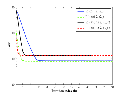
The block coordinate-descent (BCD) algorithm is adopted here to solve the batch non-convex optimization problem (P3). BCD is an iterative method which has been shown efficient in tackling large-scale optimization problems encountered with various statistical inference tasks, see e.g., [6]. The proposed solver entails an iterative procedure comprising three steps per iteration k=1,2,𝑘12k=1,2,\ldots

[S1]

Update the anomaly map:

𝐀[k+1]=argmin𝐀[12𝒫Ω(𝐘𝐏[k]𝐐[k]𝐑𝐀)F2+λ1𝐀1].𝐀delimited-[]𝑘1argsubscript𝐀12superscriptsubscriptnormsubscript𝒫Ω𝐘𝐏delimited-[]𝑘superscript𝐐delimited-[]𝑘𝐑𝐀𝐹2subscript𝜆1subscriptnorm𝐀1{\bf A}[k+1]=\mbox{arg}\>\min_{{\bf A}}\left[\frac{1}{2}\|\mathcal{P}_{\Omega}({\bf Y}-{\bf P}[k]{\bf Q}^{\prime}[k]-{\bf R}{\bf A})\|_{F}^{2}+\lambda_{1}\|{\bf A}\|_{1}\right].
[S2]

Update the nominal traffic subspace:

𝐏[k+1]=argmin𝐏[12𝒫Ω(𝐘𝐏𝐐[k]𝐑𝐀[k+1])F2+λ2𝐏F2].𝐏delimited-[]𝑘1argsubscript𝐏12superscriptsubscriptnormsubscript𝒫Ω𝐘superscript𝐏𝐐delimited-[]𝑘𝐑𝐀delimited-[]𝑘1𝐹2subscript𝜆2superscriptsubscriptnorm𝐏𝐹2{\bf P}[k+1]=\mbox{arg}\>\min_{{\bf P}}\left[\frac{1}{2}\|\mathcal{P}_{\Omega}({\bf Y}-{\bf P}{\bf Q}^{\prime}[k]-{\bf R}{\bf A}[k+1])\|_{F}^{2}+\frac{\lambda_{\ast}}{2}\|{\bf P}\|_{F}^{2}\right].
[S3]

Update the projection coefficients:

𝐐[k+1]=argmin𝐐[12𝒫Ω(𝐘𝐏[k+1]𝐐𝐑𝐀[k+1])F2+λ2𝐐F2].𝐐delimited-[]𝑘1argsubscript𝐐12superscriptsubscriptnormsubscript𝒫Ω𝐘𝐏delimited-[]𝑘1superscript𝐐𝐑𝐀delimited-[]𝑘1𝐹2subscript𝜆2superscriptsubscriptnorm𝐐𝐹2{\bf Q}[k+1]=\mbox{arg}\>\min_{{\bf Q}}\left[\frac{1}{2}\|\mathcal{P}_{\Omega}({\bf Y}-{\bf P}[k+1]{\bf Q}^{\prime}-{\bf R}{\bf A}[k+1])\|_{F}^{2}+\frac{\lambda_{\ast}}{2}\|{\bf Q}\|_{F}^{2}\right].

To update each of the variable groups, the cost of (P3) is minimized while fixing the rest of the variables to their most up-to-date values. The minimization in [S1] decomposes over the columns of 𝐀:=[𝐚1,,𝐚T]assign𝐀subscript𝐚1subscript𝐚𝑇{\bf A}:=[{\mathbf{a}}_{1},\ldots,{\mathbf{a}}_{T}]. At iteration k𝑘k, these columns are updated in parallel via Lasso

𝐚t[k+1]=argmin𝐚[12𝛀t(𝐲t𝐏[k]𝐪t[k]𝐑𝐚)22+λ1𝐚1],t=1,,Tformulae-sequencesubscript𝐚𝑡delimited-[]𝑘1subscript𝐚12superscriptsubscriptnormsubscript𝛀𝑡subscript𝐲𝑡𝐏delimited-[]𝑘subscript𝐪𝑡delimited-[]𝑘𝐑𝐚22subscript𝜆1subscriptnorm𝐚1𝑡1𝑇{\bf a}_{t}[k+1]=\arg\min_{{\bf a}}\left[\frac{1}{2}\|\mathbf{\Omega}_{t}({\bf y}_{t}-{\bf P}[k]{\bf q}_{t}[k]-{\bf R}{\bf a})\|_{2}^{2}+\lambda_{1}\|{\bf a}\|_{1}\right],\quad t=1,\ldots,T (6)

where 𝐲tsubscript𝐲𝑡{\bf y}_{t} and 𝐪t[k]subscript𝐪𝑡delimited-[]𝑘{\bf q}_{t}[k] respectively denote the t𝑡t-th column of 𝐘𝐘{\bf Y} and 𝐐[k]superscript𝐐delimited-[]𝑘{\bf Q}^{\prime}[k], while the diagonal matrix 𝛀tL×Lsubscript𝛀𝑡superscript𝐿𝐿\bm{\Omega}_{t}\in\mathbb{R}^{L\times L} contains a one on its l𝑙l-th diagonal entry if yl,tsubscript𝑦𝑙𝑡y_{l,t} is observed, and a zero otherwise. In practice, each iteration of the proposed algorithm minimizes (6) inexactly, by performing one pass of the cyclic coordinate-descent algorithm in [17, p. 92]; see Algorithm 1 for the detailed iterations. As shown at the end of this section, this inexact minimization suffices to claim convergence to a stationary point of (P3).

Similarly, in [S2] and [S3] the minimizations that give rise to 𝐏[k+1]𝐏delimited-[]𝑘1{\bf P}[k+1] and 𝐐[k+1]𝐐delimited-[]𝑘1{\bf Q}[k+1] are separable over their respective rows. For instance, the l𝑙l-th row 𝐩lsuperscriptsubscript𝐩𝑙{\bf p}_{l}^{\prime} of the traffic subspace matrix 𝐏:=[𝐩1,,𝐩L]assign𝐏superscriptsubscript𝐩1subscript𝐩𝐿{\bf P}:=[{\bf p}_{1},\ldots,{\bf p}_{L}]^{\prime} is updated as the solution of the following ridge-regression problem

𝐩l[k+1]=argmin𝐩[12((𝐲lr)𝐩𝐐[k](𝐫lr)𝐀[k+1])𝛀lr22+λ2𝐩22]subscript𝐩𝑙delimited-[]𝑘1subscript𝐩12superscriptsubscriptnormsuperscriptsuperscriptsubscript𝐲𝑙𝑟superscript𝐩superscript𝐐delimited-[]𝑘superscriptsubscriptsuperscript𝐫𝑟𝑙𝐀delimited-[]𝑘1superscriptsubscript𝛀𝑙𝑟22subscript𝜆2superscriptsubscriptnorm𝐩22\displaystyle{\bf p}_{l}[k+1]=\arg\min_{{\bf p}}\left[\frac{1}{2}\|(({\bf y}_{l}^{r})^{\prime}-{\bf p}^{\prime}{\bf Q}^{\prime}[k]-({\bf r}^{r}_{l})^{\prime}{\bf A}[k+1])\bm{\Omega}_{l}^{r}\|_{2}^{2}+\frac{\lambda_{\ast}}{2}\|{\bf p}\|_{2}^{2}\right] (7)

where (𝐲lr)superscriptsuperscriptsubscript𝐲𝑙𝑟({\bf y}_{l}^{r})^{\prime} and (𝐫lr)superscriptsubscriptsuperscript𝐫𝑟𝑙({\bf r}^{r}_{l})^{\prime} represent the l𝑙l-th row of 𝐘𝐘{\bf Y} and 𝐑𝐑{\bf R}, respectively. The t𝑡t-th diagonal entry of the diagonal matrix 𝛀lrT×Tsuperscriptsubscript𝛀𝑙𝑟superscript𝑇𝑇\bm{\Omega}_{l}^{r}\in\mathbb{R}^{T\times T} is an indicator variable testing whether measurement yl,tsubscript𝑦𝑙𝑡y_{l,t} is available. A similar regularized LS problem yields 𝐪t[k+1]subscript𝐪𝑡delimited-[]𝑘1{\bf q}_{t}[k+1], t=1,,T𝑡1𝑇t=1,\ldots,T; see Algorithm 1 for the details and a description of the overall BCD solver. The novel batch scheme for unveiling network anomalies is less complex computationally than the accelerated proximal gradient algorithm in [25], since Algorithm 1’s iterations are devoid of SVD computations.

Algorithm 1 : Batch BCD algorithm for unveiling network anomalies
  input 𝒫Ω(𝐘),Ω,𝐑,λ,subscript𝒫Ω𝐘Ω𝐑subscript𝜆\mathcal{P}_{\Omega}({\bf Y}),\Omega,{\bf R},\lambda_{*}, and λ1subscript𝜆1\lambda_{1}.
  initialize 𝐏[1]𝐏delimited-[]1{\bf P}[1] and 𝐐[1]𝐐delimited-[]1{\bf Q}[1] at random.
  for k=1,2𝑘12k=1,2,\ldots do
     [S1] Update the anomaly map:
     for f=1,,F𝑓1𝐹f=1,\ldots,F do
        𝐲~t(f)[k+1]=𝛀t(𝐲t𝐏[k]𝐪t[k]f=1f1𝐫faf,t[k+1]f=f+1F𝐫faf,t[k]),t=1,,Tformulae-sequencesuperscriptsubscript~𝐲𝑡𝑓delimited-[]𝑘1subscript𝛀𝑡subscript𝐲𝑡𝐏delimited-[]𝑘subscript𝐪𝑡delimited-[]𝑘superscriptsubscriptsuperscript𝑓1𝑓1subscript𝐫superscript𝑓subscript𝑎superscript𝑓𝑡delimited-[]𝑘1superscriptsubscriptsuperscript𝑓𝑓1𝐹subscript𝐫superscript𝑓subscript𝑎superscript𝑓𝑡delimited-[]𝑘𝑡1𝑇\tilde{{\bf y}}_{t}^{(-f)}[k+1]=\mathbf{\Omega}_{t}({\bf y}_{t}-{\bf P}[k]{\bf q}_{t}[k]-\sum_{f^{\prime}=1}^{f-1}{\bf r}_{f^{\prime}}a_{f^{\prime},t}[k+1]-\sum_{f^{\prime}=f+1}^{F}{\bf r}_{f^{\prime}}a_{f^{\prime},t}[k]),\quad t=1,\ldots,T.
        af,t[k+1]=sign(𝐫f𝐲~t(f)[k+1])[|𝐫f𝐲~t(f)[k+1]|λ1]+/𝐫f2,t=1,,Tformulae-sequencesubscript𝑎𝑓𝑡delimited-[]𝑘1signsuperscriptsubscript𝐫𝑓superscriptsubscript~𝐲𝑡𝑓delimited-[]𝑘1subscriptdelimited-[]superscriptsubscript𝐫𝑓superscriptsubscript~𝐲𝑡𝑓delimited-[]𝑘1subscript𝜆1subscriptnormsubscript𝐫𝑓2𝑡1𝑇a_{f,t}[k+1]=\textrm{sign}({\bf r}_{f}^{\prime}\tilde{{\bf y}}_{t}^{(-f)}[k+1])\big{[}|{\bf r}_{f}^{\prime}\tilde{{\bf y}}_{t}^{(-f)}[k+1]|-\lambda_{1}\big{]}_{+}/\|{\bf r}_{f}\|_{2},\quad t=1,\ldots,T.
     end for
     𝐀[k+1]=[[a1,1[k+1],,aF,1[k+1]],,[a1,T[k+1],,aF,T[k+1]]]𝐀delimited-[]𝑘1superscriptsubscript𝑎11delimited-[]𝑘1subscript𝑎𝐹1delimited-[]𝑘1superscriptsubscript𝑎1𝑇delimited-[]𝑘1subscript𝑎𝐹𝑇delimited-[]𝑘1{\bf A}[k+1]=\big{[}[a_{1,1}[k+1],\ldots,a_{F,1}[k+1]]^{\prime},\ldots,[a_{1,T}[k+1],\ldots,a_{F,T}[k+1]]^{\prime}\big{]}.
     [S2] Update the nominal traffic subspace:
     𝐩l[k+1]=(λ𝐈ρ+𝐐[k]𝛀lr𝐐[k])1𝐐[k]𝛀lr(𝐲lr𝐀[k+1]𝐫lr),l=1,,Lformulae-sequencesubscript𝐩𝑙delimited-[]𝑘1superscriptsubscript𝜆subscript𝐈𝜌superscript𝐐delimited-[]𝑘superscriptsubscript𝛀𝑙𝑟𝐐delimited-[]𝑘1superscript𝐐delimited-[]𝑘superscriptsubscript𝛀𝑙𝑟superscriptsubscript𝐲𝑙𝑟superscript𝐀delimited-[]𝑘1superscriptsubscript𝐫𝑙𝑟𝑙1𝐿{\bf p}_{l}[k+1]=\left(\lambda_{\ast}{\bf I}_{\rho}+{\bf Q}^{\prime}[k]\mathbf{\Omega}_{l}^{r}{\bf Q}[k]\right)^{-1}{\bf Q}^{\prime}[k]\mathbf{\Omega}_{l}^{r}({\bf y}_{l}^{r}-{\bf A}^{\prime}[k+1]{\bf r}_{l}^{r}),\quad l=1,\ldots,L.
     𝐏[k+1]=[𝐩1[k+1],,𝐩L[k+1]]𝐏delimited-[]𝑘1superscriptsubscript𝐩1delimited-[]𝑘1subscript𝐩𝐿delimited-[]𝑘1{\bf P}[k+1]=[{\bf p}_{1}[k+1],\ldots,{\bf p}_{L}[k+1]]^{\prime}.
     [S3] Update the projection coefficients:
     𝐪t[k+1]=(λ𝐈ρ+𝐏[k+1]𝛀t𝐏[k+1])1𝐏[k+1]𝛀t(𝐲t𝐑𝐚t[k+1]),t=1,,Tformulae-sequencesubscript𝐪𝑡delimited-[]𝑘1superscriptsubscript𝜆subscript𝐈𝜌superscript𝐏delimited-[]𝑘1subscript𝛀𝑡𝐏delimited-[]𝑘11superscript𝐏delimited-[]𝑘1subscript𝛀𝑡subscript𝐲𝑡subscript𝐑𝐚𝑡delimited-[]𝑘1𝑡1𝑇{\bf q}_{t}[k+1]=\left(\lambda_{\ast}{\bf I}_{\rho}+{\bf P}^{\prime}[k+1]\mathbf{\Omega}_{t}{\bf P}[k+1]\right)^{-1}{\bf P}^{\prime}[k+1]\mathbf{\Omega}_{t}({\bf y}_{t}-{\bf R}{\bf a}_{t}[k+1]),\quad t=1,\ldots,T.
     𝐐[k+1]=[𝐪1[k+1],,𝐪T[k+1]]𝐐delimited-[]𝑘1superscriptsubscript𝐪1delimited-[]𝑘1subscript𝐪𝑇delimited-[]𝑘1{\bf Q}[k+1]=[{\bf q}_{1}[k+1],\ldots,{\bf q}_{T}[k+1]]^{\prime}.
  end for
  return  𝐀^:=𝐀[]assign^𝐀𝐀delimited-[]\hat{{\bf A}}:={\bf A}[\infty] and 𝐗^:=𝐏[]𝐐[]assign^𝐗𝐏delimited-[]superscript𝐐delimited-[]\hat{{\bf X}}:={\bf P}[\infty]{\bf Q}^{\prime}[\infty].

Despite being non-convex and non-differentiable, (P3) has favorable structure which facilitates convergence of the iterates generated by Algorithm 1. Specifically, the resulting cost is convex in each block variable when the rest are fixed. The non-smooth 1subscript1\ell_{1}-norm is also separable over the entries of its matrix argument. Accordingly, [37, Theorem 5.1] guarantees convergence of the BCD algorithm to a stationary point of (P3). This result together with Proposition III-A establishes the next claim.

Proposition 2: If a subsequence {𝐗[k]:=𝐏[k]𝐐[k],𝐀[k]}assign𝐗delimited-[]𝑘𝐏delimited-[]𝑘superscript𝐐delimited-[]𝑘𝐀delimited-[]𝑘\{{\bf X}[k]:={\bf P}[k]{\bf Q}^{\prime}[k],{\bf A}[k]\} of iterates generated by Algorithm 1 satisfies 𝒫Ω(𝐘𝐗[k]𝐑𝐀[k])λnormsubscript𝒫Ω𝐘𝐗delimited-[]𝑘𝐑𝐀delimited-[]𝑘subscript𝜆\|\mathcal{P}_{\Omega}({\bf Y}-{\bf X}[k]-{\bf R}{\bf A}[k])\|\leq\lambda_{*}, then it converges to the optimal solution set of (P1) as k𝑘k\rightarrow\infty.

In practice, it is desirable to monitor anomalies in real time and accomodate time-varying traffic routes. These reasons motivate devising algorithms for dynamic anomalography, the subject dealt with next.

IV Dynamic Anomalography

Monitoring of large-scale IP networks necessitates collecting massive amounts of data which far outweigh the ability of modern computers to store and analyze them in real time. In addition, nonstationarities due to routing changes and missing data further challenge identification of anomalies. In dynamic networks routing tables are constantly readjusted to effect traffic load balancing and avoid congestion caused by e.g., traffic anomalies or network infrastructure failures. To account for slowly time-varing routing tables, let 𝐑tL×Fsubscript𝐑𝑡superscript𝐿𝐹{\bf R}_{t}\in\mathbb{R}^{L\times F} denote the routing matrix at time t𝑡t111Fixed size routing matrices 𝐑tsubscript𝐑𝑡{\bf R}_{t} are considered here for convenience, where L𝐿L and F𝐹F correspond to upper bounds on the number of physical links and flows transported by the network, respectively. If at time t𝑡t some links are not used at all, or, less than F𝐹F flows are present, the corresponding rows and columns of 𝐑tsubscript𝐑𝑡{\bf R}_{t} will be identically zero.. In this dynamic setting, the partially observed link counts at time t𝑡t adhere to [cf. (3)]

𝒫Ωt(𝐲t)=𝒫Ωt(𝐱t+𝐑t𝐚t+𝐯t),t=1,2,formulae-sequencesubscript𝒫subscriptΩ𝑡subscript𝐲𝑡subscript𝒫subscriptΩ𝑡subscript𝐱𝑡subscript𝐑𝑡subscript𝐚𝑡subscript𝐯𝑡𝑡12\mathcal{P}_{\Omega_{t}}({\bf y}_{t})=\mathcal{P}_{\Omega_{t}}({\bf x}_{t}+{\bf R}_{t}{\bf a}_{t}+{\bf v}_{t}),~{}t=1,2,\ldots (8)

where the link-level traffic 𝐱t:=𝐑t𝐳tassignsubscript𝐱𝑡subscript𝐑𝑡subscript𝐳𝑡{\bf x}_{t}:={\bf R}_{t}{\bf z}_{t}, for 𝐳tsubscript𝐳𝑡{\bf z}_{t} from the (low-dimensional) traffic subspace. In general, routing changes may alter a link load considerably by e.g., routing traffic completely away from a specific link. Therefore, even though the network-level traffic vectors {𝐳t}subscript𝐳𝑡\{{\bf z}_{t}\} live in a low-dimensional subspace, the same may not be true for the link-level traffic {𝐱t}subscript𝐱𝑡\{{\bf x}_{t}\} when the routing updates are major and frequent. In backbone networks however, routing changes are sporadic relative to the time-scale of data acquisition used for network monitoring tasks. For instance, data collected from the operation of Internet-2 network reveals that only a few rows of 𝐑tsubscript𝐑𝑡{\bf R}_{t} change per week [1]. It is thus safe to assume that {𝐱t}subscript𝐱𝑡\{{\bf x}_{t}\} still lies in a low-dimensional subspace, and exploit the temporal correlations of the observations to identify the anomalies.

On top of the previous arguments, in practice link measurements are acquired sequentially in time, which motivates updating previously obtained estimates rather than re-computing new ones from scratch each time a new datum becomes available. The goal is then to recursively estimate {𝐱^t,𝐚^t}subscript^𝐱𝑡subscript^𝐚𝑡\{\hat{{\bf x}}_{t},\hat{{\bf a}}_{t}\} at time t𝑡t from historical observations {𝒫Ωτ(𝐲τ),Ωτ}τ=1tsuperscriptsubscriptsubscript𝒫subscriptΩ𝜏subscript𝐲𝜏subscriptΩ𝜏𝜏1𝑡\{\mathcal{P}_{\Omega_{\tau}}({\bf y}_{\tau}),\Omega_{\tau}\}_{\tau=1}^{t}, naturally placing more importance to recent measurements. To this end, one possible adaptive counterpart to (P3) is the exponentially-weighted LS estimator found by minimizing the empirical cost

min{𝐏,𝐐,𝐀}τ=1tβtτ[12𝒫Ωτ(𝐲τ𝐏𝐪τ𝐑τ𝐚τ)22+λ2u=1tβtu𝐏F2+λ2𝐪τ22+λ1𝐚τ1]subscript𝐏𝐐𝐀superscriptsubscript𝜏1𝑡superscript𝛽𝑡𝜏delimited-[]12superscriptsubscriptnormsubscript𝒫subscriptΩ𝜏subscript𝐲𝜏subscript𝐏𝐪𝜏subscript𝐑𝜏subscript𝐚𝜏22subscript𝜆2superscriptsubscript𝑢1𝑡superscript𝛽𝑡𝑢superscriptsubscriptnorm𝐏𝐹2subscript𝜆2superscriptsubscriptnormsubscript𝐪𝜏22subscript𝜆1subscriptnormsubscript𝐚𝜏1\displaystyle\min_{\{{\bf P},{\bf Q},{\bf A}\}}\sum_{\tau=1}^{t}\beta^{t-\tau}\left[\frac{1}{2}\|\mathcal{P}_{\Omega_{\tau}}({\bf y}_{\tau}-{\bf P}{\bf q}_{\tau}-{\bf R}_{\tau}{\bf a}_{\tau})\|_{2}^{2}+\frac{\lambda_{\ast}}{2\sum_{u=1}^{t}\beta^{t-u}}\|{\bf P}\|_{F}^{2}+\frac{\lambda_{\ast}}{2}\|{\bf q}_{\tau}\|_{2}^{2}+\lambda_{1}\|{\bf a}_{\tau}\|_{1}\right] (9)

in which 0<β10𝛽10<\beta\leq 1 is the so-termed forgetting factor. When β<1𝛽1\beta<1 data in the distant past are exponentially downweighted, which facilitates tracking network anomalies in nonstationary environments. In the case of static routing (𝐑t=𝐑,t=1,2,formulae-sequencesubscript𝐑𝑡𝐑𝑡12{\bf R}_{t}={\bf R},t=1,2,\ldots) and infinite memory (β=1)𝛽1(\beta=1), the formulation (9) coincides with the batch estimator (P3). This is the reason for the time-varying factor weighting 𝐏F2superscriptsubscriptnorm𝐏𝐹2\|{\bf P}\|_{F}^{2}.

IV-A Tracking network anomalies

Towards deriving a real-time, computationally efficient, and recursive solver of (9), an alternating minimization method is adopted in which iteration k𝑘k coincides with the time scale t𝑡t of data acquisition. A justification in terms of minimizing a suitable approximate cost function is discussed in detail in Section IV-B. Per time instant t𝑡t, a new datum {𝒫Ωt(𝐲t),Ωt}subscript𝒫subscriptΩ𝑡subscript𝐲𝑡subscriptΩ𝑡\{\mathcal{P}_{\Omega_{t}}({\bf y}_{t}),\Omega_{t}\} is drawn and {𝐪t,𝐚t}subscript𝐪𝑡subscript𝐚𝑡\{{\bf q}_{t},{\bf a}_{t}\} are jointly estimated via

{𝐪[t],𝐚[t]}=argmin{𝐪,𝐚}[12𝒫Ωt(𝐲t𝐏[t1]𝐪𝐑t𝐚)22+λ2𝐪22+λ1𝐚1].𝐪delimited-[]𝑡𝐚delimited-[]𝑡subscript𝐪𝐚12superscriptsubscriptnormsubscript𝒫subscriptΩ𝑡subscript𝐲𝑡𝐏delimited-[]𝑡1𝐪subscript𝐑𝑡𝐚22subscript𝜆2superscriptsubscriptnorm𝐪22subscript𝜆1subscriptnorm𝐚1\displaystyle\{{\bf q}[t],{\bf a}[t]\}=\arg\min_{\{{\bf q},{\bf a}\}}\left[\frac{1}{2}\|\mathcal{P}_{\Omega_{t}}({\bf y}_{t}-{\bf P}[t-1]{\bf q}-{\bf R}_{t}{\bf a})\|_{2}^{2}+\frac{\lambda_{\ast}}{2}\|{\bf q}\|_{2}^{2}+\lambda_{1}\|{\bf a}\|_{1}\right]. (10)

It turns out that (10) can be efficiently solved. Fixing 𝐚𝐚{\bf a} to carry out the minimization with respect to 𝐪𝐪{\bf q} first, one is left with an 2subscript2\ell_{2}-norm regularized LS (ridge-regression) problem

𝐪[t]=𝐪delimited-[]𝑡absent\displaystyle{\bf q}[t]= argmin𝐪[12𝒫Ωt(𝐲t𝐏[t1]𝐪𝐑t𝐚)22+λ2𝐪2]subscript𝐪12superscriptsubscriptnormsubscript𝒫subscriptΩ𝑡subscript𝐲𝑡𝐏delimited-[]𝑡1𝐪subscript𝐑𝑡𝐚22subscript𝜆2superscriptnorm𝐪2\displaystyle\arg\min_{{\bf q}}\left[\frac{1}{2}\|\mathcal{P}_{\Omega_{t}}({\bf y}_{t}-{\bf P}[t-1]{\bf q}-{\bf R}_{t}{\bf a})\|_{2}^{2}+\frac{\lambda_{\ast}}{2}\|{\bf q}\|^{2}\right]
=(λ𝐈ρ+𝐏[t1]𝛀t𝐏[t1])1𝐏[t1]𝒫Ωt(𝐲t𝐑t𝐚).absentsuperscriptsubscript𝜆subscript𝐈𝜌superscript𝐏delimited-[]𝑡1subscript𝛀𝑡𝐏delimited-[]𝑡11superscript𝐏delimited-[]𝑡1subscript𝒫subscriptΩ𝑡subscript𝐲𝑡subscript𝐑𝑡𝐚\displaystyle=\left(\lambda_{\ast}{\bf I}_{\rho}+{\bf P}^{\prime}[t-1]\mathbf{\Omega}_{t}{\bf P}[t-1]\right)^{-1}{\bf P}^{\prime}[t-1]\mathcal{P}_{\Omega_{t}}({\bf y}_{t}-{\bf R}_{t}{\bf a}). (11)

Note that 𝐪[t]𝐪delimited-[]𝑡{\bf q}[t] is an affine function of 𝐚𝐚{\bf a}, and the update rule for 𝐪[t]𝐪delimited-[]𝑡{\bf q}[t] is not well defined until 𝐚𝐚{\bf a} is replaced with 𝐚[t]𝐚delimited-[]𝑡{\bf a}[t]. Towards obtaining an expression for 𝐚[t]𝐚delimited-[]𝑡{\bf a}[t], define 𝐃[t]:=(λ𝐈ρ+𝐏[t1]𝛀𝐭𝐏[t1])1𝐏[t1]assign𝐃delimited-[]𝑡superscriptsubscript𝜆subscript𝐈𝜌𝐏delimited-[]𝑡1subscript𝛀𝐭superscript𝐏delimited-[]𝑡11superscript𝐏delimited-[]𝑡1{\bf D}[t]:=\left(\lambda_{\ast}{\bf I}_{\rho}+{\bf P}[t-1]\mathbf{\Omega_{t}}{\bf P}^{\prime}[t-1]\right)^{-1}{\bf P}^{\prime}[t-1] for notational convenience, and substitute (11) back into (10) to arrive at the Lasso estimator

𝐚[t]=𝐚delimited-[]𝑡absent\displaystyle{\bf a}[t]= argmin𝐚[12𝐅[t](𝐲t𝐑t𝐚)22+λ1𝐚1]subscript𝐚12superscriptsubscriptnorm𝐅delimited-[]𝑡subscript𝐲𝑡subscript𝐑𝑡𝐚22subscript𝜆1subscriptnorm𝐚1\displaystyle\arg\min_{{\bf a}}\left[\frac{1}{2}\|{\bf F}[t]({\bf y}_{t}-{\bf R}_{t}{\bf a})\|_{2}^{2}+\lambda_{1}\|{\bf a}\|_{1}\right] (12)

where 𝐅[t]:=[𝛀t𝛀t𝐏[t1]𝐃[t]𝛀t,λ𝛀t𝐃[t]]assign𝐅delimited-[]𝑡superscriptsubscript𝛀𝑡subscript𝛀𝑡𝐏delimited-[]𝑡1𝐃delimited-[]𝑡subscript𝛀𝑡subscript𝜆subscript𝛀𝑡superscript𝐃delimited-[]𝑡{\bf F}[t]:=\left[\mathbf{\Omega}_{t}-\mathbf{\Omega}_{t}{\bf P}[t-1]{\bf D}[t]\mathbf{\Omega}_{t},\sqrt{\lambda_{\ast}}\mathbf{\Omega}_{t}{\bf D}^{\prime}[t]\right]^{\prime}. The diagonal matrix 𝛀tsubscript𝛀𝑡\bm{\Omega}_{t} was defined in Section III-B, see the discussion after (6).

In the second step of the alternating-minimization scheme, the updated subspace matrix 𝐏[t]𝐏delimited-[]𝑡{\bf P}[t] is obtained by minimizing (9) with respect to 𝐏𝐏{\bf P}, while the optimization variables {𝐪τ,𝐚τ}τ=1tsuperscriptsubscriptsubscript𝐪𝜏subscript𝐚𝜏𝜏1𝑡\{{\bf q}_{\tau},{\bf a}_{\tau}\}_{\tau=1}^{t} are fixed and take the values {𝐪[τ],𝐚[τ]}τ=1tsuperscriptsubscript𝐪delimited-[]𝜏𝐚delimited-[]𝜏𝜏1𝑡\{{\bf q}[\tau],{\bf a}[\tau]\}_{\tau=1}^{t}. This yields

𝐏[t]=argmin𝐏[λ2𝐏F2+τ=1tβtτ12𝒫Ωτ(𝐲τ𝐏𝐪[τ]𝐑τ𝐚[τ])22].𝐏delimited-[]𝑡subscript𝐏subscript𝜆2superscriptsubscriptnorm𝐏𝐹2superscriptsubscript𝜏1𝑡superscript𝛽𝑡𝜏12superscriptsubscriptnormsubscript𝒫subscriptΩ𝜏subscript𝐲𝜏𝐏𝐪delimited-[]𝜏subscript𝐑𝜏𝐚delimited-[]𝜏22\displaystyle{\bf P}[t]=\arg\min_{{\bf P}}\left[\frac{\lambda_{\ast}}{2}\|{\bf P}\|_{F}^{2}+\sum_{\tau=1}^{t}\beta^{t-\tau}\frac{1}{2}\|\mathcal{P}_{\Omega_{\tau}}({\bf y}_{\tau}-{\bf P}{\bf q}[\tau]-{\bf R}_{\tau}{\bf a}[\tau])\|_{2}^{2}\right]. (13)

Similar to the batch case, (13) decouples over the rows of 𝐏𝐏{\bf P} which are obtained in parallel via

𝐩l[t]=subscript𝐩𝑙delimited-[]𝑡absent\displaystyle{\bf p}_{l}[t]= argmin𝐩[λ2𝐩2+τ=1tβtτωl,τ(yl,τ𝐩𝐪[τ](𝐫l,τr)𝐚[τ])2],l=1,,Lformulae-sequencesubscript𝐩subscript𝜆2superscriptnorm𝐩2superscriptsubscript𝜏1𝑡superscript𝛽𝑡𝜏subscript𝜔𝑙𝜏superscriptsubscript𝑦𝑙𝜏superscript𝐩𝐪delimited-[]𝜏superscriptsuperscriptsubscript𝐫𝑙𝜏𝑟𝐚delimited-[]𝜏2𝑙1𝐿\displaystyle\arg\min_{{\bf p}}\left[\frac{\lambda_{\ast}}{2}\|{\bf p}\|^{2}+\sum_{\tau=1}^{t}\beta^{t-\tau}\omega_{l,\tau}(y_{l,\tau}-{\bf p}^{\prime}{\bf q}[\tau]-({\bf r}_{l,\tau}^{r})^{\prime}{\bf a}[\tau])^{2}\right],\quad l=1,\ldots,L (14)

where ωl,τsubscript𝜔𝑙𝜏\omega_{l,\tau} denotes the l𝑙l-th diagonal entry of 𝛀τsubscript𝛀𝜏\bm{\Omega}_{\tau}. For β=1𝛽1\beta=1, subproblems (14) can be efficiently solved using the RLS algorithm [34]. Upon defining 𝐬l[t]:=τ=1tβtτωl,τ(yl,τ𝐫l,τ𝐚[τ])𝐪[τ]assignsubscript𝐬𝑙delimited-[]𝑡superscriptsubscript𝜏1𝑡superscript𝛽𝑡𝜏subscript𝜔𝑙𝜏subscript𝑦𝑙𝜏subscriptsuperscript𝐫𝑙𝜏𝐚delimited-[]𝜏𝐪delimited-[]𝜏{\bf s}_{l}[t]:=\sum_{\tau=1}^{t}\beta^{t-\tau}\omega_{l,\tau}(y_{l,\tau}-{\bf r}^{\prime}_{l,\tau}{\bf a}[\tau]){\bf q}[\tau], 𝐇l[t]:=τ=1tβtτωl,τ𝐪[τ]𝐪[τ]+λ𝐈ρassignsubscript𝐇𝑙delimited-[]𝑡superscriptsubscript𝜏1𝑡superscript𝛽𝑡𝜏subscript𝜔𝑙𝜏𝐪delimited-[]𝜏superscript𝐪delimited-[]𝜏subscript𝜆subscript𝐈𝜌{\bf H}_{l}[t]:=\sum_{\tau=1}^{t}\beta^{t-\tau}\omega_{l,\tau}{\bf q}[\tau]{\bf q}^{\prime}[\tau]+\lambda_{\ast}{\bf I}_{\rho}, and 𝐌l[t]:=𝐇l1[t]assignsubscript𝐌𝑙delimited-[]𝑡superscriptsubscript𝐇𝑙1delimited-[]𝑡{\bf M}_{l}[t]:={\bf H}_{l}^{-1}[t], with β=1𝛽1\beta=1 one simply updates

𝐬l[t]=subscript𝐬𝑙delimited-[]𝑡absent\displaystyle{\bf s}_{l}[t]{}={} 𝐬l[t1]+ωl,t(yl,t𝐫l,t𝐚[t])𝐪[t]subscript𝐬𝑙delimited-[]𝑡1subscript𝜔𝑙𝑡subscript𝑦𝑙𝑡subscriptsuperscript𝐫𝑙𝑡𝐚delimited-[]𝑡𝐪delimited-[]𝑡\displaystyle{\bf s}_{l}[t-1]+\omega_{l,t}(y_{l,t}-{\bf r}^{\prime}_{l,t}{\bf a}[t]){\bf q}[t]
𝐌l[t]=subscript𝐌𝑙delimited-[]𝑡absent\displaystyle{\bf M}_{l}[t]{}={} 𝐌l[t1]ωl,t𝐌l[t1]𝐪[t]𝐪[t]𝐌l[t1]1+𝐪[t]𝐌l[t1]𝐪[t]subscript𝐌𝑙delimited-[]𝑡1subscript𝜔𝑙𝑡subscript𝐌𝑙delimited-[]𝑡1𝐪delimited-[]𝑡superscript𝐪delimited-[]𝑡subscript𝐌𝑙delimited-[]𝑡11superscript𝐪delimited-[]𝑡subscript𝐌𝑙delimited-[]𝑡1𝐪delimited-[]𝑡\displaystyle{\bf M}_{l}[t-1]-\omega_{l,t}\frac{{\bf M}_{l}[t-1]{\bf q}[t]{\bf q}^{\prime}[t]{\bf M}_{l}[t-1]}{1+{\bf q}^{\prime}[t]{\bf M}_{l}[t-1]{\bf q}[t]}

and forms 𝐩l[t]=𝐌l[t]𝐬l[t]subscript𝐩𝑙delimited-[]𝑡subscript𝐌𝑙delimited-[]𝑡subscript𝐬𝑙delimited-[]𝑡{\bf p}_{l}[t]={\bf M}_{l}[t]{\bf s}_{l}[t], for l=1,,L𝑙1𝐿l=1,\ldots,L.

However, for 0<β<10𝛽10<\beta<1 the regularization term (λ/2)𝐩2subscript𝜆2superscriptnorm𝐩2(\lambda_{\ast}/2)\|{\bf p}\|^{2} in (14) makes it impossible to express 𝐇l[t]subscript𝐇𝑙delimited-[]𝑡{\bf H}_{l}[t] in terms of 𝐇l[t1]subscript𝐇𝑙delimited-[]𝑡1{\bf H}_{l}[t-1] plus a rank-one correction. Hence, one cannot resort to the matrix inversion lemma and update 𝐌l[t]subscript𝐌𝑙delimited-[]𝑡{\bf M}_{l}[t] with quadratic complexity only. Based on direct inversion of 𝐇l[t]subscript𝐇𝑙delimited-[]𝑡{\bf H}_{l}[t], l=1,,L𝑙1𝐿l=1,\ldots,L, the overall recursive algorithm for tracking network anomalies is tabulated under Algorithm 2. The per iteration cost of the L𝐿L inversions (each 𝒪(ρ3)𝒪superscript𝜌3\mathcal{O}(\rho^{3}), which could be further reduced if one leverages also the symmetry of 𝐇l[t]subscript𝐇𝑙delimited-[]𝑡{\bf H}_{l}[t]) is affordable for moderate number of links, because ρ𝜌\rho is small when estimating low-rank traffic matrices. Still, for those settings where computational complexity reductions are at a premium, an online stochastic gradient descent algorithm is described in Section V-A.

Algorithm 2 : Online algorithm for tracking network anomalies
  input {𝒫Ωt(𝐲t),𝛀t,𝐑t}t=1,β,λ,superscriptsubscriptsubscript𝒫subscriptΩ𝑡subscript𝐲𝑡subscript𝛀𝑡subscript𝐑𝑡𝑡1𝛽subscript𝜆\{\mathcal{P}_{\Omega_{t}}({\bf y}_{t}),\mathbf{\Omega}_{t},{\bf R}_{t}\}_{t=1}^{\infty},\beta,\lambda_{\ast}, and λ1subscript𝜆1\lambda_{1}.
  initialize 𝐆l[0]=𝟎ρ×ρsubscript𝐆𝑙delimited-[]0subscript0𝜌𝜌{\bf G}_{l}[0]=\mathbf{0}_{\rho\times\rho}, 𝐬l[0]=𝟎ρ,l=1,,Lformulae-sequencesubscript𝐬𝑙delimited-[]0subscript0𝜌𝑙1𝐿{\bf s}_{l}[0]=\mathbf{0}_{\rho},~{}l=1,...,L, and 𝐏[0]𝐏delimited-[]0{\bf P}[0] at random.
  for t=1,2𝑡12t=1,2,\ldots do
     𝐃[t]=(λ𝐈ρ+𝐏[t1]𝛀t𝐏[t1])1𝐏[t1]𝐃delimited-[]𝑡superscriptsubscript𝜆subscript𝐈𝜌superscript𝐏delimited-[]𝑡1subscript𝛀𝑡𝐏delimited-[]𝑡11superscript𝐏delimited-[]𝑡1{\bf D}[t]=\left(\lambda_{\ast}{\bf I}_{\rho}+{\bf P}^{\prime}[t-1]\mathbf{\Omega}_{t}{\bf P}[t-1]\right)^{-1}{\bf P}^{\prime}[t-1].
     𝐅[t]=[𝛀t𝛀t𝐏[t1]𝐃[t]𝛀t,λ𝛀t𝐃[t]]𝐅delimited-[]𝑡superscriptsubscript𝛀𝑡subscript𝛀𝑡𝐏delimited-[]𝑡1𝐃delimited-[]𝑡subscript𝛀𝑡subscript𝜆subscript𝛀𝑡superscript𝐃delimited-[]𝑡{\bf F}[t]=\left[\mathbf{\Omega}_{t}-\mathbf{\Omega}_{t}{\bf P}[t-1]{\bf D}[t]\mathbf{\Omega}_{t},\sqrt{\lambda_{\ast}}\mathbf{\Omega}_{t}{\bf D}^{\prime}[t]\right]^{\prime}.
     𝐚[t]=argmin𝐚[12𝐅[t](𝐲t𝐑t𝐚)2+λ1𝐚1]𝐚delimited-[]𝑡subscript𝐚12superscriptnorm𝐅delimited-[]𝑡subscript𝐲𝑡subscript𝐑𝑡𝐚2subscript𝜆1subscriptnorm𝐚1{\bf a}[t]=\arg\min_{{\bf a}}\left[\frac{1}{2}\|{\bf F}[t]({\bf y}_{t}-{\bf R}_{t}{\bf a})\|^{2}+\lambda_{1}\|{\bf a}\|_{1}\right].
     𝐪[t]=𝐃[t]𝛀t(𝐲t𝐑t𝐚[t])𝐪delimited-[]𝑡𝐃delimited-[]𝑡subscript𝛀𝑡subscript𝐲𝑡subscript𝐑𝑡𝐚delimited-[]𝑡{\bf q}[t]={\bf D}[t]\mathbf{\Omega}_{t}({\bf y}_{t}-{\bf R}_{t}{\bf a}[t]).
     𝐆l[t]=β𝐆l[t1]+ωl,t𝐪[t]𝐪[t],l=1,,Lformulae-sequencesubscript𝐆𝑙delimited-[]𝑡𝛽subscript𝐆𝑙delimited-[]𝑡1subscript𝜔𝑙𝑡𝐪delimited-[]𝑡𝐪superscriptdelimited-[]𝑡𝑙1𝐿{\bf G}_{l}[t]=\beta{\bf G}_{l}[t-1]+\omega_{l,t}{\bf q}[t]{\bf q}[t]^{\prime},\quad l=1,\ldots,L.
     𝐬l[t]=β𝐬l[t1]+ωl,t(yl,t𝐫l,t𝐚[t])𝐪[t],l=1,,Lformulae-sequencesubscript𝐬𝑙delimited-[]𝑡𝛽subscript𝐬𝑙delimited-[]𝑡1subscript𝜔𝑙𝑡subscript𝑦𝑙𝑡subscriptsuperscript𝐫𝑙𝑡𝐚delimited-[]𝑡𝐪delimited-[]𝑡𝑙1𝐿{\bf s}_{l}[t]=\beta{\bf s}_{l}[t-1]+\omega_{l,t}(y_{l,t}-{\bf r}^{\prime}_{l,t}{\bf a}[t]){\bf q}[t],\quad l=1,\ldots,L.
     𝐩l[t]=(𝐆l[t]+λ𝐈ρ)1𝐬l[t],l=1,,Lformulae-sequencesubscript𝐩𝑙delimited-[]𝑡superscriptsubscript𝐆𝑙delimited-[]𝑡subscript𝜆subscript𝐈𝜌1subscript𝐬𝑙delimited-[]𝑡𝑙1𝐿{\bf p}_{l}[t]=\left({\bf G}_{l}[t]+\lambda_{\ast}{\bf I}_{\rho}\right)^{-1}{\bf s}_{l}[t],\quad l=1,...,L.
     return  𝐚^t:=𝐚[t]assignsubscript^𝐚𝑡𝐚delimited-[]𝑡\hat{{\bf a}}_{t}:={\bf a}[t] and 𝐱^t:=𝐏[t]𝐪[t]assignsubscript^𝐱𝑡𝐏delimited-[]𝑡𝐪delimited-[]𝑡\hat{{\bf x}}_{t}:={\bf P}[t]{\bf q}[t].
  end for
Remark 2 (Robust subspace trackers)

Algorithm 2 is closely related to timely robust subspace trackers, which aim at estimating a low-rank subspace 𝐏𝐏{\bf P} from grossly corrupted and possibly incomplete data, namely 𝒫Ωt(𝐲t)=𝒫Ωt(𝐏𝐪t+𝐚t+𝐯t),t=1,2,formulae-sequencesubscript𝒫subscriptΩ𝑡subscript𝐲𝑡subscript𝒫subscriptΩ𝑡subscript𝐏𝐪𝑡subscript𝐚𝑡subscript𝐯𝑡𝑡12\mathcal{P}_{\Omega_{t}}({\bf y}_{t})=\mathcal{P}_{\Omega_{t}}({\bf P}{\bf q}_{t}+{\bf a}_{t}+{\bf v}_{t}),~{}t=1,2,\ldots. In the absence of sparse ‘outliers’ {𝐚t}t=1superscriptsubscriptsubscript𝐚𝑡𝑡1\{{\bf a}_{t}\}_{t=1}^{\infty}, an online algorithm based on incremental gradient descent on the Grassmannian manifold of subspaces was put forth in [4]. The second-order RLS-type algorithm in [15] extends the seminal projection approximation subspace tracking algorithm [39] to handle missing data. When outliers are present, robust counterparts can be found in [14, 18, 26]. Relative to all aforementioned works, the estimation problem here is more challenging due to the presence of the fat (compression) matrix 𝐑tsubscript𝐑𝑡{\bf R}_{t}; see [25] for fundamental identifiability issues related to the model (3).

IV-B Convergence Analysis

This section studies the convergence of the iterates generated by Algorithm 2, for the infinite memory special case i.e., when β=1𝛽1\beta=1. Upon defining the function

gt(𝐏,𝐪,𝐚):=12𝒫Ωt(𝐲t𝐏𝐪𝐑t𝐚)22+λ2𝐪22+λ1𝐚1assignsubscript𝑔𝑡𝐏𝐪𝐚12superscriptsubscriptnormsubscript𝒫subscriptΩ𝑡subscript𝐲𝑡𝐏𝐪subscript𝐑𝑡𝐚22subscript𝜆2superscriptsubscriptnorm𝐪22subscript𝜆1subscriptnorm𝐚1\displaystyle g_{t}({\bf P},{\bf q},{\bf a}):=\frac{1}{2}\|\mathcal{P}_{\Omega_{t}}({\bf y}_{t}-{\bf P}{\bf q}-{\bf R}_{t}{\bf a})\|_{2}^{2}+\frac{\lambda_{\ast}}{2}\|{\bf q}\|_{2}^{2}+\lambda_{1}\|{\bf a}\|_{1}

in addition to t(𝐏):=min{𝐪,𝐚}gt(𝐏,𝐪,𝐚)assignsubscript𝑡𝐏subscript𝐪𝐚subscript𝑔𝑡𝐏𝐪𝐚\ell_{t}({\bf P}):=\min_{\{{\bf q},{\bf a}\}}g_{t}({\bf P},{\bf q},{\bf a}), the online solver of Section IV-A aims at minimizing the following average cost function at time t𝑡t

Ct(𝐏):=1tτ=1tτ(𝐏)+λ2t𝐏F2.assignsubscript𝐶𝑡𝐏1𝑡superscriptsubscript𝜏1𝑡subscript𝜏𝐏subscript𝜆2𝑡superscriptsubscriptnorm𝐏𝐹2\displaystyle C_{t}({\bf P}):=\frac{1}{t}\sum_{\tau=1}^{t}\ell_{\tau}({\bf P})+\frac{\lambda_{\ast}}{2t}\|{\bf P}\|_{F}^{2}. (15)

Normalization (by t𝑡t) ensures that the cost function does not grow unbounded as time evolves. For any finite t𝑡t, (15) it is essentially identical to the batch estimator in (P3) up to a scaling, which does not affect the value of the minimizers. Note that as time evolves, minimization of Ctsubscript𝐶𝑡C_{t} becomes increasingly complex computationally. Even evaluating Ctsubscript𝐶𝑡C_{t} is challenging for large t𝑡t, since it entails solving t𝑡t Lasso problems to minimize all gτsubscript𝑔𝜏g_{\tau} and define the functions τsubscript𝜏\ell_{\tau}, τ=1,,T𝜏1𝑇\tau=1,\ldots,T. Hence, at time t𝑡t the subspace estimate 𝐏[t]𝐏delimited-[]𝑡{\bf P}[t] is obtained by minimizing the approximate cost function

C^t(𝐏)=1tτ=1tgτ(𝐏,𝐪[τ],𝐚[τ])+λ2t𝐏F2subscript^𝐶𝑡𝐏1𝑡superscriptsubscript𝜏1𝑡subscript𝑔𝜏𝐏𝐪delimited-[]𝜏𝐚delimited-[]𝜏subscript𝜆2𝑡superscriptsubscriptnorm𝐏𝐹2\displaystyle\hat{C}_{t}({\bf P})=\frac{1}{t}\sum_{\tau=1}^{t}g_{\tau}({\bf P},{\bf q}[\tau],{\bf a}[\tau])+\frac{\lambda_{\ast}}{2t}\|{\bf P}\|_{F}^{2} (16)

in which {𝐪[t],𝐚[t]}𝐪delimited-[]𝑡𝐚delimited-[]𝑡\{{\bf q}[t],{\bf a}[t]\} are obtained based on the prior subspace estimate 𝐏[t1]𝐏delimited-[]𝑡1{\bf P}[t-1] after solving [cf. (10)]

{𝐪[t],𝐚[t]}=argmin{𝐪,𝐚}gt(𝐏[t1],𝐪,𝐚).𝐪delimited-[]𝑡𝐚delimited-[]𝑡subscript𝐪𝐚subscript𝑔𝑡𝐏delimited-[]𝑡1𝐪𝐚\displaystyle\{{\bf q}[t],{\bf a}[t]\}=\arg\min_{\{{\bf q},{\bf a}\}}g_{t}({\bf P}[t-1],{\bf q},{\bf a}). (17)

Obtaining 𝐪[t]𝐪delimited-[]𝑡{\bf q}[t] this way resembles the projection approximation adopted in [39], and can only be evaluated after 𝐚[t]𝐚delimited-[]𝑡{\bf a}[t] is obtained [cf. (11)]. Since C^t(𝐏)subscript^𝐶𝑡𝐏\hat{C}_{t}({\bf P}) is a smooth convex function, the minimizer 𝐏[t]=argmin𝐏C^t(𝐏)𝐏delimited-[]𝑡subscript𝐏subscript^𝐶𝑡𝐏{\bf P}[t]=\arg\min_{{\bf P}}\hat{C}_{t}({\bf P}) is the solution of the quadratic equation C^t(𝐏[t])=𝟎L×ρsubscript^𝐶𝑡𝐏delimited-[]𝑡subscript0𝐿𝜌\nabla\hat{C}_{t}({\bf P}[t])=\mathbf{0}_{L\times\rho}.

So far, it is apparent that the approximate cost function C^t(𝐏[t])subscript^𝐶𝑡𝐏delimited-[]𝑡\hat{C}_{t}({\bf P}[t]) overestimates the target cost Ct(𝐏[t])subscript𝐶𝑡𝐏delimited-[]𝑡C_{t}({\bf P}[t]), for t=1,2,𝑡12t=1,2,\ldots. However, it is not clear whether the dictionary iterates {𝐏[t]}t=1superscriptsubscript𝐏delimited-[]𝑡𝑡1\{{\bf P}[t]\}_{t=1}^{\infty} converge, and most importantly, how well can they optimize the target cost function Ctsubscript𝐶𝑡C_{t}. The good news is that C^t(𝐏[t])subscript^𝐶𝑡𝐏delimited-[]𝑡\hat{C}_{t}({\bf P}[t]) asymptotically approaches Ct(𝐏[t])subscript𝐶𝑡𝐏delimited-[]𝑡C_{t}({\bf P}[t]), and the subspace iterates null Ct(𝐏[t])subscript𝐶𝑡𝐏delimited-[]𝑡\nabla C_{t}({\bf P}[t]) as well, both as t𝑡t\to\infty. The latter result is summarized in the next proposition, which is proved in the next section.

Proposition 3: Assume that: a1) {Ωt}t=1superscriptsubscriptsubscriptΩ𝑡𝑡1\{\Omega_{t}\}_{t=1}^{\infty} and {𝐲t}t=1superscriptsubscriptsubscript𝐲𝑡𝑡1\{{\bf y}_{t}\}_{t=1}^{\infty} are independent and identically distributed (i.i.d.) random processes; a2) 𝒫Ωt(𝐲t)subscriptnormsubscript𝒫subscriptΩ𝑡subscript𝐲𝑡\|\mathcal{P}_{\Omega_{t}}({\bf y}_{t})\|_{\infty} is uniformly bounded; a3) iterates {𝐏[t]}t=1superscriptsubscript𝐏delimited-[]𝑡𝑡1\{{\bf P}[t]\}_{t=1}^{\infty} are in a compact set L×ρsuperscript𝐿𝜌\mathcal{L}\subset\mathbb{R}^{L\times\rho}; a4) C^t(𝐏)subscript^𝐶𝑡𝐏\hat{C}_{t}({\bf P}) is positive definite, namely λmin[2C^t(𝐏)]csubscript𝜆delimited-[]superscript2subscript^𝐶𝑡𝐏𝑐\lambda_{\min}\left[\nabla^{2}\hat{C}_{t}({\bf P})\right]\geq c for some c>0𝑐0c>0; and a5) the Lasso (12) has a unique solution. Then limtCt(𝐏[t])=𝟎L×ρsubscript𝑡subscript𝐶𝑡𝐏delimited-[]𝑡subscript0𝐿𝜌\lim_{t\rightarrow\infty}\nabla C_{t}({\bf P}[t])=\mathbf{0}_{L\times\rho} almost surely (a.s.), i.e., the subspace iterates {𝐏[t]}t=1superscriptsubscript𝐏delimited-[]𝑡𝑡1\{{\bf P}[t]\}_{t=1}^{\infty} asymptotically coincide with the stationary points of the batch problem (P3).

To clearly delineate the scope of the analysis, it is worth commenting on the assumptions a1)-a5) and the factors that influence their satisfaction. Regarding a1), the acquired data is assumed statistically independent across time as it is customary when studying the stability and performance of online (adaptive) algorithms [34]. Still, in accordance with the adaptive filtering folklore, as β1𝛽1\beta\to 1 the upshot of the analysis based on i.i.d. data extends accurately to the pragmatic setting whereby the link-counts and missing data patterns exhibit spatiotemporal correlations. Uniform boundedness of 𝒫Ωt(𝐲t)subscript𝒫subscriptΩ𝑡subscript𝐲𝑡\mathcal{P}_{\Omega_{t}}({\bf y}_{t}) [cf. a2)] is satisfied in practice, since the traffic is always limited by the (finite) capacity of the physical links. The bounded subspace requirement in a3) is a technical assumption that simplifies the arguments of the ensuing proof, and has been corroborated via computer simulations. It is apparent that the sampling set ΩtsubscriptΩ𝑡\Omega_{t} plays a key role towards ensuring that a4) and a5) are satisfied. Intuitively, if the missing entries tend to be only few and somehow uniformly distributed across links and time, they will not markedly increase coherence of the regression matrices 𝐅[t]𝐑t𝐅delimited-[]𝑡subscript𝐑𝑡{\bf F}[t]{\bf R}_{t}, and thus compromise the uniqueness of the Lasso solutions. This also increases the likelihood that 2C^t(𝐏)=λt𝐈Lρ+1tτ=1t(𝐪[τ]𝐪[τ])𝛀τc𝐈Lρsuperscript2subscript^𝐶𝑡𝐏subscript𝜆𝑡subscript𝐈𝐿𝜌1𝑡superscriptsubscript𝜏1𝑡tensor-product𝐪delimited-[]𝜏superscript𝐪delimited-[]𝜏subscript𝛀𝜏succeeds-or-equals𝑐subscript𝐈𝐿𝜌\nabla^{2}\hat{C}_{t}({\bf P})=\frac{\lambda_{\ast}}{t}{\bf I}_{L\rho}+\frac{1}{t}\sum_{\tau=1}^{t}({\bf q}[\tau]{\bf q}^{\prime}[\tau])\otimes\mathbf{\Omega}_{\tau}\succeq c{\bf I}_{L\rho} holds. As argued in [23], if needed one could incorporate additional regularization terms in the cost function to enforce a4) and a5). Before moving on to the proof, a remark is in order.

Remark 3 (Performance guarantees)

In line with Proposition 1, one may be prompted to ponder whether the online estimator offers the performance guarantees of the nuclear-norm regularized estimator (P1), for which stable/exact recovery have been well documented e.g., in [25, 42, 8]. Specifically, given the learned traffic subspace 𝐏¯¯𝐏\bar{{\bf P}} and the corresponding 𝐐¯¯𝐐\bar{{\bf Q}} and 𝐀¯¯𝐀\bar{{\bf A}} [obtained via (10)] over a time window of size T𝑇T, is {𝐗^:=𝐏¯𝐐¯,𝐀^:=𝐀¯}formulae-sequenceassign^𝐗¯𝐏superscript¯𝐐assign^𝐀¯𝐀\{\hat{{\bf X}}:=\bar{{\bf P}}\bar{{\bf Q}}^{\prime},\hat{{\bf A}}:=\bar{{\bf A}}\} an optimal solution of (P1) when T𝑇T\rightarrow\infty? This in turn requires asymptotic analysis of the optimality conditions for (P1), and is left for future research. Nevertheless, empirically the online estimator attains the performance of (P1), as evidenced by the numerical tests in Section VI.

IV-C Proof of Proposition IV-B

The main steps of the proof are inspired by [23], which studies convergence of an online dictionary learning algorithm using the theory of martingale sequences; see e.g., [22]. However, relative to [23] the problem here introduces several distinct elements including: i) missing data with a time-varying pattern ΩtsubscriptΩ𝑡\Omega_{t}; ii) a non-convex bilinear term where the tall subspace matrix 𝐏𝐏{\bf P} plays a role similar to the fat dictionary in [23], but the multiplicative projection coefficients here are not sparse; and iii) the additional bilinear terms 𝐑t𝐚tsubscript𝐑𝑡subscript𝐚𝑡{\bf R}_{t}{\bf a}_{t} which entail sparse coding of 𝐚tsubscript𝐚𝑡{\bf a}_{t} as in [23], but with a known regression (routing) matrix. Hence, convergence analysis becomes more challenging and demands, in part, for a new treatment. Accordingly, in the sequel emphasis will be placed on the novel aspects specific to the problem at hand.

The basic structure of the proof consists of three preliminary lemmata, which are subsequently used to establish that limtCt(𝐏[t])=𝟎L×ρsubscript𝑡subscript𝐶𝑡𝐏delimited-[]𝑡subscript0𝐿𝜌\lim_{t\rightarrow\infty}\nabla C_{t}({\bf P}[t])=\mathbf{0}_{L\times\rho} a.s. through a simple argument. The first lemma deals with regularity properties of functions C^tsubscript^𝐶𝑡\hat{C}_{t} and Ctsubscript𝐶𝑡C_{t}, which will come handy later on; see Appendix A for a proof.

Lemma 1: If a2) and a5) hold, then the functions: i) {𝐚t(𝐏),𝐪t(𝐏)}=argmin{𝐪,𝐚}gt(𝐏,𝐪,𝐚)subscript𝐚𝑡𝐏subscript𝐪𝑡𝐏subscript𝐪𝐚subscript𝑔𝑡𝐏𝐪𝐚\{{\bf a}_{t}({\bf P}),{\bf q}_{t}({\bf P})\}=\arg\min_{\{{\bf q},{\bf a}\}}g_{t}({\bf P},{\bf q},{\bf a}), ii) gt(𝐏,𝐪[t],𝐚[t])subscript𝑔𝑡𝐏𝐪delimited-[]𝑡𝐚delimited-[]𝑡g_{t}({\bf P},{\bf q}[t],{\bf a}[t]), iii) t(𝐏)subscript𝑡𝐏\ell_{t}({\bf P}), and iv) t(𝐏)subscript𝑡𝐏\nabla\ell_{t}({\bf P}) are Lipschitz continuous for 𝐏𝐏{\bf P}\in\mathcal{L} (\mathcal{L} is a compact set), with constants independent of t𝑡t.

The next lemma (proved in Appendix B) asserts that the distance between two subsequent traffic subspace estimates vanishes as t𝑡t\to\infty, a property that will be instrumental later on when establishing that C^t(𝐏[t])Ct(𝐏[t])0subscript^𝐶𝑡𝐏delimited-[]𝑡subscript𝐶𝑡𝐏delimited-[]𝑡0\hat{C}_{t}({\bf P}[t])-C_{t}({\bf P}[t])\to 0 a.s.

Lemma 2: If a2)-a5) hold, then 𝐏[t+1]𝐏[t]F=𝒪(1/t)subscriptnorm𝐏delimited-[]𝑡1𝐏delimited-[]𝑡𝐹𝒪1𝑡\|{\bf P}[t+1]-{\bf P}[t]\|_{F}=\mathcal{O}(1/t).

The previous lemma by no means implies that the subspace iterates converge, which is a much more ambitious objective that may not even hold under the current assumptions. The final lemma however, asserts that the cost sequence indeed converges with probability one; see Appendix C for a proof.

Lemma 3: If a1)-a5) hold, then C^t(𝐏[t])subscript^𝐶𝑡𝐏delimited-[]𝑡\hat{C}_{t}({\bf P}[t]) converges a.s. Moreover, C^t(𝐏[t])Ct(𝐏[t])0subscript^𝐶𝑡𝐏delimited-[]𝑡subscript𝐶𝑡𝐏delimited-[]𝑡0\hat{C}_{t}({\bf P}[t])-C_{t}({\bf P}[t])\to 0 a.s.

Putting the pieces together, in the sequel it is shown that the sequence {C^t(𝐏[t])Ct(𝐏[t])}t=1superscriptsubscriptsubscript^𝐶𝑡𝐏delimited-[]𝑡subscript𝐶𝑡𝐏delimited-[]𝑡𝑡1\{\nabla\hat{C}_{t}({\bf P}[t])-\nabla C_{t}({\bf P}[t])\}_{t=1}^{\infty} converges a.s. to zero, and since C^t(𝐏[t])=𝟎L×ρsubscript^𝐶𝑡𝐏delimited-[]𝑡subscript0𝐿𝜌\nabla\hat{C}_{t}({\bf P}[t])=\mathbf{0}_{L\times\rho} by algorithmic construction, the subspace iterates {𝐏[t]}t=1superscriptsubscript𝐏delimited-[]𝑡𝑡1\{{\bf P}[t]\}_{t=1}^{\infty} coincide with the stationary points of the target cost function Ctsubscript𝐶𝑡C_{t}. To this end, it suffices to prove that every convergent subsequence nulls the gradient Ctsubscript𝐶𝑡\nabla C_{t} asymptotically, which in turn implies that the entire sequence converges to the set of stationary points of the batch problem (P3).

Since \mathcal{L} is compact by virtue of a3), one can always pick a convergent subsequence {𝐏[t]}t=1superscriptsubscript𝐏delimited-[]𝑡𝑡1\{{\bf P}[t]\}_{t=1}^{\infty} whose limit point is 𝐏superscript𝐏{\bf P}^{*}, say222Formally, the subsequence should be denoted as {𝐏[t(i)]}i=1superscriptsubscript𝐏delimited-[]𝑡𝑖𝑖1\{{\bf P}[t(i)]\}_{i=1}^{\infty}, but a slight abuse of notation is allowed for simplicity.. Consider the positive-valued decreasing sequence {αt}t=1superscriptsubscriptsubscript𝛼𝑡𝑡1\{\alpha_{t}\}_{t=1}^{\infty} (that necessarily converges to zero), and recall that C^t(𝐏[t]+αt𝐔)Ct(𝐏[t]+αt𝐔)subscript^𝐶𝑡𝐏delimited-[]𝑡subscript𝛼𝑡𝐔subscript𝐶𝑡𝐏delimited-[]𝑡subscript𝛼𝑡𝐔\hat{C}_{t}({\bf P}[t]+\alpha_{t}{\bf U})\geq C_{t}({\bf P}[t]+\alpha_{t}{\bf U}) for any 𝐔L×ρ𝐔superscript𝐿𝜌{\bf U}\in\mathbb{R}^{L\times\rho}. From the mean-value theorem and for arbitrary 𝐔𝐔{\bf U}, expanding both sides of the inequality around the point 𝐏[t]𝐏delimited-[]𝑡{\bf P}[t] one arrives at

C^t(𝐏[t])+αttr{𝐔C^t(𝐏[t])}+12αt2tr{𝐔2C^t(𝚯1)𝐔}subscript^𝐶𝑡𝐏delimited-[]𝑡subscript𝛼𝑡trsuperscript𝐔subscript^𝐶𝑡𝐏delimited-[]𝑡12superscriptsubscript𝛼𝑡2trsuperscript𝐔superscript2subscript^𝐶𝑡subscript𝚯1𝐔absent\displaystyle\hat{C}_{t}({\bf P}[t])+\alpha_{t}\text{tr}\{{\bf U}^{\prime}\nabla\hat{C}_{t}({\bf P}[t])\}+\frac{1}{2}\alpha_{t}^{2}\text{tr}\{{\bf U}^{\prime}\nabla^{2}\hat{C}_{t}(\mathbf{\Theta}_{1}){\bf U}\}\geq
Ct(𝐏[t])+αttr{𝐔Ct(𝐏[t])}+12αt2tr{𝐔2Ct(𝚯2)𝐔}subscript𝐶𝑡𝐏delimited-[]𝑡subscript𝛼𝑡trsuperscript𝐔subscript𝐶𝑡𝐏delimited-[]𝑡12superscriptsubscript𝛼𝑡2trsuperscript𝐔superscript2subscript𝐶𝑡subscript𝚯2𝐔\displaystyle\hskip 156.49014ptC_{t}({\bf P}[t])+\alpha_{t}\text{tr}\{{\bf U}^{\prime}\nabla C_{t}({\bf P}[t])\}+\frac{1}{2}\alpha_{t}^{2}\text{tr}\{{\bf U}^{\prime}\nabla^{2}C_{t}(\mathbf{\Theta}_{2}){\bf U}\}

for some 𝚯1,𝚯2L×ρsubscript𝚯1subscript𝚯2superscript𝐿𝜌\mathbf{\Theta}_{1},\mathbf{\Theta}_{2}\in\mathbb{R}^{L\times\rho} and all t𝑡t. Taking limit as t𝑡t\to\infty and applying Lemma IV-C it follows that

limttr{𝐔(C^t(𝐏[t])Ct(𝐏[t]))}+limt12αttr{𝐔(2C^t(𝚯1)2Ct(𝚯2))𝐔}0.subscript𝑡trsuperscript𝐔subscript^𝐶𝑡𝐏delimited-[]𝑡subscript𝐶𝑡𝐏delimited-[]𝑡subscript𝑡12subscript𝛼𝑡trsuperscript𝐔superscript2subscript^𝐶𝑡subscript𝚯1superscript2subscript𝐶𝑡subscript𝚯2𝐔0\displaystyle\lim_{t\rightarrow\infty}\text{tr}\{{\bf U}^{\prime}(\nabla\hat{C}_{t}({\bf P}[t])-\nabla C_{t}({\bf P}[t]))\}+\lim_{t\rightarrow\infty}\frac{1}{2}\alpha_{t}\text{tr}\{{\bf U}^{\prime}(\nabla^{2}\hat{C}_{t}(\mathbf{\Theta}_{1})-\nabla^{2}C_{t}(\mathbf{\Theta}_{2})){\bf U}\}\geq 0. (18)

One can readily show that 2C^t(𝚯1)=1tτ=1t(𝐪[τ]𝐪[τ])𝛀τ+λt𝐈Lρsuperscript2subscript^𝐶𝑡subscript𝚯11𝑡superscriptsubscript𝜏1𝑡tensor-product𝐪delimited-[]𝜏superscript𝐪delimited-[]𝜏subscript𝛀𝜏subscript𝜆𝑡subscript𝐈𝐿𝜌\nabla^{2}\hat{C}_{t}(\mathbf{\Theta}_{1})=\frac{1}{t}\sum_{\tau=1}^{t}({\bf q}[\tau]{\bf q}^{\prime}[\tau])\otimes\mathbf{\Omega}_{\tau}+\frac{\lambda_{\ast}}{t}{\bf I}_{L\rho} is bounded since 𝐏[t]𝐏delimited-[]𝑡{\bf P}[t] is uniformly bounded [cf. a2)]. Consequently, limt12αttr{𝐔(2C^t(𝚯1))𝐔}=0subscript𝑡12subscript𝛼𝑡trsuperscript𝐔superscript2subscript^𝐶𝑡subscript𝚯1𝐔0\lim_{t\rightarrow\infty}\frac{1}{2}\alpha_{t}\text{tr}\{{\bf U}^{\prime}(\nabla^{2}\hat{C}_{t}(\mathbf{\Theta}_{1})){\bf U}\}=0. Furthermore, since τsubscript𝜏\nabla\ell_{\tau} is Lipschitz as per Lemma IV-C, Ctsubscript𝐶𝑡\nabla C_{t} is Lipschitz as well and it follows that limt12αttr{𝐔2Ct(𝚯2)𝐔}=0subscript𝑡12subscript𝛼𝑡trsuperscript𝐔superscript2subscript𝐶𝑡subscript𝚯2𝐔0\lim_{t\rightarrow\infty}\frac{1}{2}\alpha_{t}\text{tr}\{{\bf U}^{\prime}\nabla^{2}C_{t}(\mathbf{\Theta}_{2}){\bf U}\}=0. All in all, the second term in (18) vanishes and one is left with

limttr{𝐔(C^t(𝐏t)Ct(𝐏t))}0.subscript𝑡trsuperscript𝐔subscript^𝐶𝑡subscript𝐏𝑡subscript𝐶𝑡subscript𝐏𝑡0\displaystyle\lim_{t\rightarrow\infty}\text{tr}\{{\bf U}^{\prime}(\nabla\hat{C}_{t}({\bf P}_{t})-\nabla C_{t}({\bf P}_{t}))\}\geq 0. (19)

Because 𝐔L×ρ𝐔superscript𝐿𝜌{\bf U}\in\mathbb{R}^{L\times\rho} is arbitrary, (19) can only hold if limt(C^t(𝐏[t])Ct(𝐏[t]))=𝟎L×ρsubscript𝑡subscript^𝐶𝑡𝐏delimited-[]𝑡subscript𝐶𝑡𝐏delimited-[]𝑡subscript0𝐿𝜌\lim_{t\rightarrow\infty}(\nabla\hat{C}_{t}({\bf P}[t])-\nabla C_{t}({\bf P}[t]))=\mathbf{0}_{L\times\rho} a.s., which completes the proof. \blacksquare

V Further Algorithmic Issues

For completeness, this section outlines a couple of additional algorithmic aspects relevant to anomaly detection in large-scale networks. Firstly, a lightweight first-order algorithm is developed as an alternative to Algorithm 2, which relies on fast Nesterov-type gradient updates for the traffic subspace. Secondly, the possibility of developing distributed algorithms for dynamic anomalography is discussed.

V-A Fast stochastic-gradient algorithm

Reduction of the computational complexity in updating the traffic subspace 𝐏𝐏{\bf P} is the subject of this section. The basic alternating minimization framework in Section IV-A will be retained, and the updates for {𝐪[t],𝐚[t]}𝐪delimited-[]𝑡𝐚delimited-[]𝑡\{{\bf q}[t],{\bf a}[t]\} will be identical to those tabulated under Algorithm 2. However, instead of solving an unconstrained quadratic program per iteration to obtain 𝐏[t]𝐏delimited-[]𝑡{\bf P}[t] [cf. (13)], the refinements to the subspace estimate will be given by a (stochastic) gradient algorithm.

As discussed in Section IV-B, in Algorithm 2 the subspace estimate 𝐏[t]𝐏delimited-[]𝑡{\bf P}[t] is obtained by minimizing the empirical cost function C^t(𝐏)=(1/t)τ=1tfτ(𝐏)subscript^𝐶𝑡𝐏1𝑡superscriptsubscript𝜏1𝑡subscript𝑓𝜏𝐏\hat{C}_{t}({\bf P})=(1/t)\sum_{\tau=1}^{t}f_{\tau}({\bf P}), where

ft(𝐏):=12𝛀t(𝐲t𝐏𝐪[t]𝐑t𝐚[t])22+λ2t𝐏F2+λ2𝐪[t]22+λ1𝐚[t]1,t=1,2,formulae-sequenceassignsubscript𝑓𝑡𝐏12superscriptsubscriptnormsubscript𝛀𝑡subscript𝐲𝑡𝐏𝐪delimited-[]𝑡subscript𝐑𝑡𝐚delimited-[]𝑡22subscript𝜆2𝑡superscriptsubscriptnorm𝐏𝐹2subscript𝜆2superscriptsubscriptnorm𝐪delimited-[]𝑡22subscript𝜆1subscriptnorm𝐚delimited-[]𝑡1𝑡12f_{t}({\bf P}):=\frac{1}{2}\|\bm{\Omega}_{t}({\mathbf{y}}_{t}-{\bf P}{\mathbf{q}}[t]-{\bf R}_{t}{\mathbf{a}}[t])\|_{2}^{2}+\frac{\lambda_{*}}{2t}\|{\bf P}\|_{F}^{2}+\frac{\lambda_{\ast}}{2}\|{\bf q}[t]\|_{2}^{2}+\lambda_{1}\|{\bf a}[t]\|_{1},\quad t=1,2,\ldots (20)

By the law of large numbers, if data {𝒫Ωt(𝐲t)}t=1superscriptsubscriptsubscript𝒫subscriptΩ𝑡subscript𝐲𝑡𝑡1\{\mathcal{P}_{\Omega_{t}}({\bf y}_{t})\}_{t=1}^{\infty} are stationary, solving min𝐏limtC^t(𝐏)subscript𝐏subscript𝑡subscript^𝐶𝑡𝐏\min_{{\bf P}}\lim_{t\to\infty}\hat{C}_{t}({\bf P}) yields the desired minimizer of the expected cost 𝔼[Ct(𝐏)]𝔼delimited-[]subscript𝐶𝑡𝐏\mathbb{E}[C_{t}({\bf P})], where the expectation is taken with respect to the unknown probability distribution of the data. A standard approach to achieve this same goal – typically with reduced computational complexity – is to drop the expectation (or the sample averaging operator for that matter), and update the nominal traffic subspace via a stochastic gradient iteration [34]

𝐏[t]=𝐏delimited-[]𝑡absent\displaystyle{\bf P}[t]{}={} argmin𝐏Q(1/μ~[t]),t(𝐏,𝐏[t1])subscript𝐏subscript𝑄1~𝜇delimited-[]𝑡𝑡𝐏𝐏delimited-[]𝑡1\displaystyle\arg\min_{{\bf P}}Q_{(1/\tilde{\mu}[t]),t}({\bf P},{\bf P}[t-1])
=\displaystyle={} 𝐏[t1]μ~[t]ft(𝐏[t1])𝐏delimited-[]𝑡1~𝜇delimited-[]𝑡subscript𝑓𝑡𝐏delimited-[]𝑡1\displaystyle{\bf P}[t-1]-\tilde{\mu}[t]\nabla f_{t}({\bf P}[t-1]) (21)

where μ~[t]~𝜇delimited-[]𝑡\tilde{\mu}[t] is a stepsize, Qμ,t(𝐏1,𝐏2):=ft(𝐏2)+𝐏1𝐏2,ft(𝐏2)+μ2𝐏1𝐏2f2assignsubscript𝑄𝜇𝑡subscript𝐏1subscript𝐏2subscript𝑓𝑡subscript𝐏2subscript𝐏1subscript𝐏2subscript𝑓𝑡subscript𝐏2𝜇2superscriptsubscriptnormsubscript𝐏1subscript𝐏2𝑓2Q_{\mu,t}({\bf P}_{1},{\bf P}_{2}):=f_{t}({\bf P}_{2})+\langle{\bf P}_{1}-{\bf P}_{2},\nabla f_{t}({\bf P}_{2})\rangle+\frac{\mu}{2}\|{\bf P}_{1}-{\bf P}_{2}\|_{f}^{2}, and ft(𝐏)=𝛀t(𝐲t𝐏𝐪[t]𝐑t𝐚[t])𝐪[t]+(λ/t)𝐏subscript𝑓𝑡𝐏subscript𝛀𝑡subscript𝐲𝑡𝐏𝐪delimited-[]𝑡subscript𝐑𝑡𝐚delimited-[]𝑡superscript𝐪delimited-[]𝑡subscript𝜆𝑡𝐏\nabla f_{t}({\bf P})=-\bm{\Omega}_{t}({\mathbf{y}}_{t}-{\bf P}{\mathbf{q}}[t]-{\bf R}_{t}{\mathbf{a}}[t]){\mathbf{q}}^{\prime}[t]+(\lambda_{*}/t){\bf P}. In the context of adaptive filtering, stochastic gradient algorithms such as (20) are known to converge typically slower than RLS. This is expected since RLS can be shown to be an instance of Newton’s (second-order) optimization method [34].

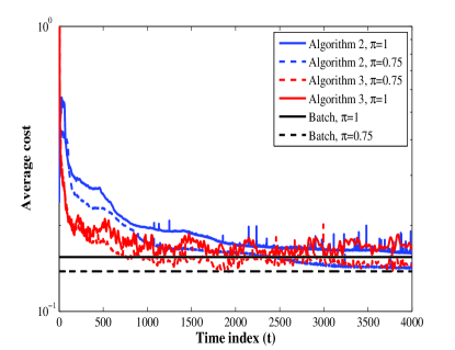
Building on the increasingly popular accelerated gradient methods for (batch) smooth optimization [29, 5], the idea here is to speed-up the learning rate of the estimated traffic subspace (V-A), without paying a penalty in terms of computational complexity per iteration. The critical difference between standard gradient algorithms and the so-termed Nesterov’s variant, is that the accelerated updates take the form 𝐏[t]=𝐏~[t]μ~[t]ft(𝐏~[t])𝐏delimited-[]𝑡~𝐏delimited-[]𝑡~𝜇delimited-[]𝑡subscript𝑓𝑡~𝐏delimited-[]𝑡{\bf P}[t]=\tilde{\bf P}[t]-\tilde{\mu}[t]\nabla f_{t}(\tilde{\bf P}[t]), which relies on a judicious linear combination 𝐏~[t1]~𝐏delimited-[]𝑡1\tilde{\bf P}[t-1] of the previous pair of iterates {𝐏[t1],𝐏[t2]}𝐏delimited-[]𝑡1𝐏delimited-[]𝑡2\{{\bf P}[t-1],{\bf P}[t-2]\}. Specifically, the choice 𝐏~[t]=𝐏[t1]+k[t1]1k[t](𝐏[t1]𝐏[t2])~𝐏delimited-[]𝑡𝐏delimited-[]𝑡1𝑘delimited-[]𝑡11𝑘delimited-[]𝑡𝐏delimited-[]𝑡1𝐏delimited-[]𝑡2\tilde{\bf P}[t]={\bf P}[t-1]+\frac{k[t-1]-1}{k[t]}\left({\bf P}[t-1]-{\bf P}[t-2]\right), where k[t]=[1+4k2[t1]+1]/2𝑘delimited-[]𝑡delimited-[]14superscript𝑘2delimited-[]𝑡112k[t]=\left[1+\sqrt{4k^{2}[t-1]+1}\right]/2, has been shown to significantly accelerate batch gradient algorithms resulting in convergence rate no worse than 𝒪(1/k2)𝒪1superscript𝑘2\mathcal{O}(1/k^{2}); see e.g., [5] and references therein. Using this acceleration technique in conjunction with a backtracking stepsize rule [6], a fast online stochastic gradient algorithm for unveiling network anomalies is tabulated under Algorithm 3. Different from Algorithm 2, no matrix inversions are involved in the update of the traffic subspace 𝐏[t]𝐏delimited-[]𝑡{\bf P}[t]. Clearly, a standard (non accelerated) stochastic gradient descent algorithm with backtracking stepsize rule is subsumed as a special case, when k[t]=1𝑘delimited-[]𝑡1k[t]=1, t=0,1,2,𝑡012t=0,1,2,\ldots

Algorithm 3 : Online stochastic gradient algorithm for unveiling network anomalies
  input {𝐲t,𝐑t,𝛀t}t=1,superscriptsubscriptsubscript𝐲𝑡subscript𝐑𝑡subscript𝛀𝑡𝑡1\{{\mathbf{y}}_{t},{\bf R}_{t},\bm{\Omega}_{t}\}_{t=1}^{\infty}, ρ,λ,λ1,η>1𝜌subscript𝜆subscript𝜆1𝜂1\rho,\lambda_{*},\lambda_{1},\eta>1.
  initialize 𝐏[0]𝐏delimited-[]0{\bf P}[0] at random, μ[0]>0𝜇delimited-[]00\mu[0]>0, 𝐏~[1]:=𝐏[0]assign~𝐏delimited-[]1𝐏delimited-[]0\tilde{\bf P}[1]:={\bf P}[0], and k[1]:=1assign𝑘delimited-[]11k[1]:=1.
  for t=1,2𝑡12t=1,2,\ldots do
     𝐃[t]=(λ𝐈ρ+𝐏[t1]𝛀t𝐏[t1])1𝐏[t1]𝐃delimited-[]𝑡superscriptsubscript𝜆subscript𝐈𝜌superscript𝐏delimited-[]𝑡1subscript𝛀𝑡𝐏delimited-[]𝑡11superscript𝐏delimited-[]𝑡1{\bf D}[t]=\left(\lambda_{\ast}{\bf I}_{\rho}+{\bf P}^{\prime}[t-1]\mathbf{\Omega}_{t}{\bf P}[t-1]\right)^{-1}{\bf P}^{\prime}[t-1]
     𝐅[t]:=[𝛀t𝛀t𝐏[t1]𝐃[t]𝛀t,λ𝛀t𝐃[t]]assignsuperscript𝐅delimited-[]𝑡subscript𝛀𝑡subscript𝛀𝑡𝐏delimited-[]𝑡1𝐃delimited-[]𝑡subscript𝛀𝑡subscript𝜆subscript𝛀𝑡superscript𝐃delimited-[]𝑡{\bf F}^{\prime}[t]:=\left[\mathbf{\Omega}_{t}-\mathbf{\Omega}_{t}{\bf P}[t-1]{\bf D}[t]\mathbf{\Omega}_{t},\sqrt{\lambda_{\ast}}\mathbf{\Omega}_{t}{\bf D}^{\prime}[t]\right]
     𝐚[t]=argmin𝐚[12𝐅[t](𝐲t𝐑t𝐚)2+λ1𝐚1]𝐚delimited-[]𝑡subscript𝐚12superscriptnorm𝐅delimited-[]𝑡subscript𝐲𝑡subscript𝐑𝑡𝐚2subscript𝜆1subscriptnorm𝐚1{\bf a}[t]=\arg\min_{{\bf a}}\left[\frac{1}{2}\|{\bf F}[t]({\bf y}_{t}-{\bf R}_{t}{\bf a})\|^{2}+\lambda_{1}\|{\bf a}\|_{1}\right]
     𝐪[t]=𝐃[t]𝛀t(𝐲t𝐑t𝐚t)𝐪delimited-[]𝑡𝐃delimited-[]𝑡subscript𝛀𝑡subscript𝐲𝑡subscript𝐑𝑡subscript𝐚𝑡{\bf q}[t]={\bf D}[t]\mathbf{\Omega}_{t}({\bf y}_{t}-{\bf R}_{t}{\bf a}_{t})
     Find the smallest nonnegative integer i[t]𝑖delimited-[]𝑡i[t] such that with μ¯:=ηi[t]μ[t1]assign¯𝜇superscript𝜂𝑖delimited-[]𝑡𝜇delimited-[]𝑡1\bar{\mu}:=\eta^{i[t]}\mu[t-1]
ft(𝐏~[t](1/μ¯)ft(𝐏~[t]))Qμ¯,t(𝐏~[t](1/μ¯)ft(𝐏~[t]),𝐏~[t])subscript𝑓𝑡~𝐏delimited-[]𝑡1¯𝜇subscript𝑓𝑡~𝐏delimited-[]𝑡subscript𝑄¯𝜇𝑡~𝐏delimited-[]𝑡1¯𝜇subscript𝑓𝑡~𝐏delimited-[]𝑡~𝐏delimited-[]𝑡f_{t}(\tilde{\bf P}[t]-(1/\bar{\mu})\nabla f_{t}(\tilde{\bf P}[t]))\leq Q_{\bar{\mu},t}(\tilde{\bf P}[t]-(1/\bar{\mu})\nabla f_{t}(\tilde{\bf P}[t]),\tilde{\bf P}[t])
holds, and set μ[t]=ηi[t]μ[t1].𝜇delimited-[]𝑡superscript𝜂𝑖delimited-[]𝑡𝜇delimited-[]𝑡1\mu[t]=\eta^{i[t]}\mu[t-1].
     𝐏[t]=𝐏~[t](1/μ[t])ft(𝐏~[t]).𝐏delimited-[]𝑡~𝐏delimited-[]𝑡1𝜇delimited-[]𝑡subscript𝑓𝑡~𝐏delimited-[]𝑡{\bf P}[t]=\tilde{\bf P}[t]-(1/\mu[t])\nabla f_{t}(\tilde{\bf P}[t]).
     k[t+1]=1+1+4k2[t]2.𝑘delimited-[]𝑡1114superscript𝑘2delimited-[]𝑡2k[t+1]=\frac{1+\sqrt{1+4k^{2}[t]}}{2}.
     𝐏~[t+1]=𝐏[t]+(k[t]1k[t+1])(𝐏[t]𝐏[t1]).~𝐏delimited-[]𝑡1𝐏delimited-[]𝑡𝑘delimited-[]𝑡1𝑘delimited-[]𝑡1𝐏delimited-[]𝑡𝐏delimited-[]𝑡1\tilde{\bf P}[t+1]={\bf P}[t]+\left(\frac{k[t]-1}{k[t+1]}\right)({\bf P}[t]-{\bf P}[t-1]).
  end for
  return  𝐱^[t]:=𝐏[t]𝐪[t],𝐚^[t]:=𝐚[t]formulae-sequenceassign^𝐱delimited-[]𝑡𝐏delimited-[]𝑡𝐪delimited-[]𝑡assign^𝐚delimited-[]𝑡𝐚delimited-[]𝑡\hat{{\mathbf{x}}}[t]:={\bf P}[t]{\mathbf{q}}[t],\hat{{\mathbf{a}}}[t]:={\mathbf{a}}[t].

Convergence analysis of Algorithm 3 is beyond the scope of this paper, and will only be corroborated using computer simulations in Section VI. It is worth pointing out that since a non-diminishing stepsize is adopted, asymptotically the iterates generated by Algorithm 3 will hover inside a ball centered at the minimizer of the expected cost, with radius proportional to the noise variance.

V-B In-network anomaly trackers

Implementing Algorithms 1-3 presumes that network nodes continuously communicate their local link traffic measurements to a central monitoring station, which uses their aggregation in {𝒫Ωt(𝐲t)}t=1superscriptsubscriptsubscript𝒫subscriptΩ𝑡subscript𝐲𝑡𝑡1\{\mathcal{P}_{\Omega_{t}}({\bf y}_{t})\}_{t=1}^{\infty} to unveil network anomalies. While for the most part this is the prevailing operational paradigm adopted in current network technologies, it is fair to say there are limitations associated with this architecture. For instance, collecting all this information centrally may lead to excessive protocol overhead, especially when the rate of data acquisition is high at the routers. Moreover, minimizing the exchanges of raw measurements may be desirable to reduce unavoidable communication errors that translate to missing data. Performing the optimization in a centralized fashion raises robustness concerns as well, since the central monitoring station represents an isolated point of failure.

These reasons motivate devising fully-distributed iterative algorithms for dynamic anomalography in large-scale networks, embedding the network anomaly detection functionality to the routers. In a nutshell, per iteration nodes carry out simple computational tasks locally, relying on their own link count measurements (a few entries of the network-wide vector 𝐲tsubscript𝐲𝑡{\mathbf{y}}_{t} corresponding to the router links). Subsequently, local estimates are refined after exchanging messages only with directly connected neighbors, which facilitates percolation of local information to the whole network. The end goal is for network nodes to consent on a global map of network anomalies, and attain (or at least come close to) the estimation performance of the centralized counterpart which has all data {𝒫Ωt(𝐲t)}t=1superscriptsubscriptsubscript𝒫subscriptΩ𝑡subscript𝐲𝑡𝑡1\{\mathcal{P}_{\Omega_{t}}({\bf y}_{t})\}_{t=1}^{\infty} available.

Relying on the alternating-directions method of multipliers (AD-MoM) as the basic tool to carry out distributed optimization, a general framework for in-network sparsity-regularized rank minimization was put forth in a companion paper [24]. In the context of network anomaly detection, results therein are encouraging yet there is ample room for improvement and immediate venues for future research open up. For instance, the distributed algorithms of [24] can only tackle the batch formulation (P3), so extensions to a dynamic network setting, e.g., building on the ideas here to devise distributed anomaly trackers seems natural. To obtain desirable tradeoffs in terms of computational complexity and speed of convergence, developing and studying algorithms for distributed optimization based on Nesterov’s acceleration techniques emerges as an exciting and rather pristine research direction; see [19] for early work dealing with separable batch optimization.

VI Performance Tests

Performance of the proposed batch and online estimators is assessed in this section via computer simulations using both synthetic and real network data.
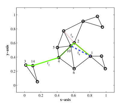
Refer to caption

Figure 1: Synthetic network topology graph, and the paths used for routing three flows.

VI-A Synthetic network data tests

Synthetic network example. A network of N=15𝑁15N=15 nodes is considered as a realization of the random geometric graph model with agents randomly placed on the unit square, and two agents link if their Euclidean distance is less than a prescribed communication range of dc=0.35subscript𝑑𝑐0.35d_{c}=0.35; see Fig. 1. The network graph is bidirectional and comprises L=52𝐿52L=52 links, and F=N(N1)=210𝐹𝑁𝑁1210F=N(N-1)=210 OD flows. For each candidate OD pair, minimum hop count routing is considered to form the routing matrix 𝐑𝐑{\bf R}. Entries of 𝐯tsubscript𝐯𝑡{\bf v}_{t} are i.i.d., zero-mean, Gaussian with variance σ2superscript𝜎2\sigma^{2}; i.e., vl,t𝒩(0,σ2)similar-tosubscript𝑣𝑙𝑡𝒩0superscript𝜎2v_{l,t}\sim\mathcal{N}(0,\sigma^{2}). Flow-traffic vectors 𝐳tsubscript𝐳𝑡{\bf z}_{t} are generated from the low-dimensional subspace 𝐔F×r𝐔superscript𝐹𝑟{\bf U}\in\mathbb{R}^{F\times r} with i.i.d. entries uf,i𝒩(0,1/F)similar-tosubscript𝑢𝑓𝑖𝒩01𝐹u_{f,i}\sim\mathcal{N}(0,1/F), and projection coefficients wi,tN(0,1)similar-tosubscript𝑤𝑖𝑡𝑁01w_{i,t}\sim N(0,1) such that 𝐳t=𝐔𝐰tsubscript𝐳𝑡subscript𝐔𝐰𝑡{\bf z}_{t}={\bf U}{\bf w}_{t}. Every entry of 𝐚tsubscript𝐚𝑡{\bf a}_{t} is randomly drawn from the set {1,0,1}101\{-1,0,1\}, with Pr(af,t=1)=Pr(af,t=1)=p/2Prsubscript𝑎𝑓𝑡1Prsubscript𝑎𝑓𝑡1𝑝2{\rm Pr}(a_{f,t}=-1)={\rm Pr}(a_{f,t}=1)=p/2. Entries of 𝐘𝐘{\bf Y} are sampled uniformly at random with probability π𝜋\pi to form the diagonal sampling matrix 𝛀tsubscript𝛀𝑡\mathbf{\Omega}_{t}. The observations at time instant t𝑡t are generated according to 𝒫Ωt(𝐲t)=𝛀t(𝐑𝐳t+𝐑𝐚t+𝐯t)subscript𝒫subscriptΩ𝑡subscript𝐲𝑡subscript𝛀𝑡subscript𝐑𝐳𝑡subscript𝐑𝐚𝑡subscript𝐯𝑡\mathcal{P}_{\Omega_{t}}({\bf y}_{t})=\mathbf{\Omega}_{t}({\bf R}{\bf z}_{t}+{\bf R}{\bf a}_{t}+{\bf v}_{t}). Unless otherwise stated, r=2𝑟2r=2, ρ=5𝜌5\rho=5, and β=0.99𝛽0.99\beta=0.99 are used throughout. Different values of σ𝜎\sigma, p𝑝p and π𝜋\pi are tested.

Refer to caption Refer to caption
(a) (b)
Figure 2: Performance of the batch estimator (P3), for σ=102𝜎superscript102\sigma=10^{-2} and p=0.005𝑝0.005p=0.005. (a) Cost of the estimators (P1) and (P3), versus iteration index. (b) Amplitude of the true and estimated anomalies for π=1𝜋1\pi=1 (no missing data), when PFA=0.0011subscript𝑃FA0.0011P_{\rm FA}=0.0011 and PD=0.947subscript𝑃D0.947P_{\rm D}=0.947.

Performance of the batch estimator. To demonstrate the merits of the batch BCD algorithm for unveiling network anomalies (Algorithm 1), simulated data are generated for a time interval of size T=100𝑇100T=100. For validation purposes, the benchmark estimator (P1) is iteratively solved by alternating minimization over 𝐀𝐀{\bf A} (which corresponds to Lasso) and 𝐗𝐗{\bf X}. The minimizations with respect to 𝐗𝐗{\bf X} can be carried out using the iterative singular-value thresholding (SVT) algorithm [7]. Note that with full data, SVT requires only a single SVD computation. In the presence of missing data however, the SVT algorithm may require several SVD computations until convergence, rendering the said algorithm prohibitively complex for large-scale problems. In contrast, Algorithm 1 only requires simple ρ×ρ𝜌𝜌\rho\times\rho inversions. Fig. 2 (a) depicts the convergence of the respective algorithms used to solve (P1) and (P3), for different amounts of missing data (controlled by π𝜋\pi). It is apparent that both estimators attain identical performance after a few tens of iterations, as asserted by Proposition III-A. To corroborate the effectiveness of Algorithm 1 in unveiling network anomalies across flows and time, Fig. 2 (b) maps out the magnitude of the true and estimated anomalies when σ=102𝜎superscript102\sigma=10^{-2} and π=1𝜋1\pi=1. To discard spurious estimates, consider the hypothesis test a^f,t010.1superscriptsubscriptgreater-than-or-equals-or-less-thansubscript0subscript1subscript^𝑎𝑓𝑡0.1\hat{a}_{f,t}\gtreqless_{\mathcal{H}_{0}}^{\mathcal{H}_{1}}0.1, with anomalous and anomaly-free hypotheses 1subscript1\mathcal{H}_{1} and 0subscript0\mathcal{H}_{0}, respectively. The false alarm and detection rates achieved are then PFA=0.0011subscript𝑃FA0.0011P_{\rm FA}=0.0011 and PD=0.947subscript𝑃D0.947P_{\rm D}=0.947, respectively.

Refer to caption Refer to caption
(a) (b)
Figure 3: Performance of the online estimator for σ=102𝜎superscript102\sigma=10^{-2}, p=0.005𝑝0.005p=0.005, λ1=0.11subscript𝜆10.11\lambda_{1}=0.11, and λ=0.36subscript𝜆0.36\lambda_{*}=0.36. (a) Evolution of the average cost Ct(𝐏[t])subscript𝐶𝑡𝐏delimited-[]𝑡C_{t}({\bf P}[t]) of the online algorithms versus the batch counterpart (P3). (b) Amplitude of true (solid) and estimated (circle markers) anomalies via the online Algorithm 2, for three representative flows when π=1𝜋1\pi=1 (no missing data).

Performance of the online algorithms. To confirm the convergence and effectiveness of the online Algorithms 2 and 3, simulation tests are carried out for infinite memory β=1𝛽1\beta=1 and invariant routing matrix 𝐑𝐑{\bf R}. Figure 3 (a) depicts the evolutions of the average cost Ct(𝐏t)subscript𝐶𝑡subscript𝐏𝑡C_{t}({\bf P}_{t}) in (15) for different amounts of missing data π=0.75,1𝜋0.751\pi=0.75,1 when the noise level is σ=102𝜎superscript102\sigma=10^{-2}. It is evident that for both online algorithms the average cost converges (possibly within a ball) to its batch counterpart in (P3) normalized by the window size T=t𝑇𝑡T=t. Impressively, this observation together with the one in Fig. 2 (a) corroborate that the online estimators can attain the performance of the benchmark estimator, whose stable/exact recovery performance is well documented e.g., in [25, 42, 9]. It is further observed that the more data are missing, the more time it takes to learn the low-rank nominal traffic subspace, which in turn slows down convergence.

To examine the tracking capability of the online estimators, Fig. 3 (b) depicts the estimated versus true anomalies over time as Algorithm 2 evolves for three representative flows indicated on Fig. 1, namely f2,f6,f9subscript𝑓2subscript𝑓6subscript𝑓9f_{2},f_{6},f_{9} corresponding to the f=2,6,9𝑓269f=2,6,9-th rows of 𝐀0subscript𝐀0{\bf A}_{0}. Setting the detection threshold to the value 0.10.10.1 as before, for the flows f2,f6,f9subscript𝑓2subscript𝑓6subscript𝑓9f_{2},f_{6},f_{9} Algorithm 2 attains detection rate PD=0.83,1,1subscript𝑃D0.8311P_{\rm D}=0.83,1,1 at false alarm rate PFA=0.0171,0.0040,0.0081subscript𝑃FA0.01710.00400.0081P_{\rm{FA}}=0.0171,0.0040,0.0081, respectively. The quantification error per flow is also around PQ=0.7606,0.5863,0.4028subscript𝑃Q0.76060.58630.4028P_{\rm Q}=0.7606,0.5863,0.4028, respectively. As expected, more false alarms are declared at early iterations as the low-rank subspace has not been learnt accurately. Upon learning the subspace performance improves and almost all anomalies are identified. Careful inspection of Fig. 3 (b) reveals that the anomalies for f9subscript𝑓9f_{9} are better identified visually than those for f2subscript𝑓2f_{2}. As shown in Fig. 1, f2subscript𝑓2f_{2} is carried over links (1,2),(2,4),(4,14),(14,3)1224414143(1,2),(2,4),(4,14),(14,3) each one carrying 33,31,35,223331352233,31,35,22 additional flows, respectively, whereas f9subscript𝑓9f_{9} is aggregated over link (1,3)13(1,3) with only 222 additional flows. Hence, identifying f2subscript𝑓2f_{2}’s anomalies from the highly-superimposed load of links (1,2),(2,4),(4,14),(14,3)1224414143(1,2),(2,4),(4,14),(14,3) is a more challenging task relative to link (1,3)13(1,3). This simple example manifests the fact that the detection performance strongly depends on the network topology and the routing policy implemented, which determine the routing matrix. In accordance with [25], the coherence of sparse column subsets of the routing matrix plays an important role in identifying the anomalies. In essence, the more incoherent the column subsets of 𝐑𝐑{\bf R} are, the better recovery performance one can attain. An intriguing question left here to address in future research pertains to desirable network topologies giving rise to incoherent routing matrices.

Tracking routing changes. The measurement model in (8) has two time-varying attributes which challenge the identification of anomalies. The first one is missing measurement data arising from e.g., packet losses during the data collection process, and the second one pertains to routing changes due to e.g., network congestion or link failures. It is thus important to test whether the proposed online algorithm succeeds in tracking these changes. As discussed earlier, missing data are sampled uniformly at random. To assess the impact of routing changes on the recovery performance, a simple probabilistic model is adopted where each time instant a single link fails, or, returns to the operational state. Let 𝚽𝚽{\bf\Phi} denote the adjacency matrix of the network graph G𝐺G, where [𝚽]i,j=1subscriptdelimited-[]𝚽𝑖𝑗1[{\bf\Phi}]_{i,j}=1 if there exists a physical link joining nodes i𝑖i and j𝑗j, and zero otherwise. Similarly, the active links involved in routing the data at time t𝑡t are represented by the effective adjacency matrix 𝚽teffsuperscriptsubscript𝚽𝑡eff{\bf\Phi}_{t}^{\rm{eff}}. At time instant t+1𝑡1t+1, a biased coin is tossed with small success probability α𝛼\alpha, and one of the links, say (i,j)𝚽teff𝑖𝑗superscriptsubscript𝚽𝑡eff(i,j)\in{\bf\Phi}_{t}^{\rm{eff}}, is chosen uniformly at random and removed from G𝐺G while ensuring that the network remains connected. Likewise, an edge (,k)𝚽\𝚽teff𝑘\𝚽superscriptsubscript𝚽𝑡eff(\ell,k)\in{\bf\Phi}\backslash{\bf\Phi}_{t}^{\rm{eff}} is added with the same probability α𝛼\alpha. The resulting adjacency matrix is then 𝚽t+1eff=𝚽teff+𝟙{b1,t}𝐞𝐞k𝟙{b1,t}𝐞i𝐞jsuperscriptsubscript𝚽𝑡1effsuperscriptsubscript𝚽𝑡effsubscript1subscript𝑏1𝑡subscript𝐞subscriptsuperscript𝐞𝑘subscript1subscript𝑏1𝑡subscript𝐞𝑖subscriptsuperscript𝐞𝑗{\bf\Phi}_{t+1}^{\rm{eff}}={\bf\Phi}_{t}^{\rm{eff}}+\mathds{1}_{\{b_{1,t}\}}{\bf e}_{\ell}{\bf e}^{\prime}_{k}-\mathds{1}_{\{b_{1,t}\}}{\bf e}_{i}{\bf e}^{\prime}_{j}, where the indicator function 𝟙{x𝒳}subscript1𝑥𝒳\mathds{1}_{\{x\in\mathcal{X}\}} equals one when x𝒳𝑥𝒳x\in\mathcal{X}, and zero otherwise; and b1,t,b2,tBer(α)similar-tosubscript𝑏1𝑡subscript𝑏2𝑡Ber𝛼b_{1,t},b_{2,t}\sim\textrm{Ber}(\alpha) are i.i.d. Bernoulli random variables. The minimum hop-count algorithm is then applied to 𝚽t+1effsuperscriptsubscript𝚽𝑡1eff{\bf\Phi}_{t+1}^{\rm{eff}}, to update the routing matrix 𝐑t+1subscript𝐑𝑡1{\bf R}_{t+1}. Note that 𝐑t+1=𝐑tsubscript𝐑𝑡1subscript𝐑𝑡{\bf R}_{t+1}={\bf R}_{t} with probability (1α)2superscript1𝛼2(1-\alpha)^{2}.

Refer to caption Refer to caption
(a) (b)
Refer to caption Refer to caption
(c) (d)
Figure 4: Tracking routing changes for p=0.005𝑝0.005p=0.005. (a) Evolution of average anomaly (dotted) and traffic (solid) estimation errors. (b) Evolution of average detection (solid) and false alarm (dotted) rates. (c) Estimated (red) versus true (blue) link traffic for three representative links. (d) Estimated (circle markers) versus true (solid) anomalies for three representative flows when π=0.8𝜋0.8\pi=0.8, σ=105𝜎superscript105\sigma=10^{-5}, and α=0.01𝛼0.01\alpha=0.01.

The performance is tested here for fast and slowly varying routing corresponding to α=0.1𝛼0.1\alpha=0.1 and α=0.01𝛼0.01\alpha=0.01, respectively, when β=0.9𝛽0.9\beta=0.9. A metric of interest is the average square error in estimating the anomalies, namely eta:=1ti=1t𝐚^t𝐚t22assignsuperscriptsubscript𝑒𝑡𝑎1𝑡superscriptsubscript𝑖1𝑡superscriptsubscriptnormsubscript^𝐚𝑡subscript𝐚𝑡22e_{t}^{a}:=\frac{1}{t}\sum_{i=1}^{t}\|\hat{{\bf a}}_{t}-{\bf a}_{t}\|_{2}^{2}, and the link traffic, namely etx:=1ti=1t𝐱^t𝐱t22assignsuperscriptsubscript𝑒𝑡𝑥1𝑡superscriptsubscript𝑖1𝑡superscriptsubscriptnormsubscript^𝐱𝑡subscript𝐱𝑡22e_{t}^{x}:=\frac{1}{t}\sum_{i=1}^{t}\|\hat{{\bf x}}_{t}-{\bf x}_{t}\|_{2}^{2}. Fig. 4 (a) plots the average estimation error for various noise variances and amounts of missing data. The estimation error decreases quickly and after learning the subspace it becomes almost invariant. To evaluate the support recovery performance of the online estimator, define the average detection and false alarm rate

PD:=τ=1tf=1F𝟙{a^f,τ0.1,af,τ0.1}τ=1tf=1F𝟙{af,τ0.1},PFA:=τ=1tf=1F𝟙{a^f,τ0.1,af,τ0.1}τ=1tf=1F𝟙{af,τ0.1}.formulae-sequenceassignsubscript𝑃Dsuperscriptsubscript𝜏1𝑡superscriptsubscript𝑓1𝐹subscript1formulae-sequencesubscript^𝑎𝑓𝜏0.1subscript𝑎𝑓𝜏0.1superscriptsubscript𝜏1𝑡superscriptsubscript𝑓1𝐹subscript1subscript𝑎𝑓𝜏0.1assignsubscript𝑃FAsuperscriptsubscript𝜏1𝑡superscriptsubscript𝑓1𝐹subscript1formulae-sequencesubscript^𝑎𝑓𝜏0.1subscript𝑎𝑓𝜏0.1superscriptsubscript𝜏1𝑡superscriptsubscript𝑓1𝐹subscript1subscript𝑎𝑓𝜏0.1\displaystyle P_{\rm D}:=\frac{\sum_{\tau=1}^{t}\sum_{f=1}^{F}\mathds{1}_{\{\hat{a}_{f,\tau}\geq 0.1,a_{f,\tau}\geq 0.1\}}}{\sum_{\tau=1}^{t}\sum_{f=1}^{F}\mathds{1}_{\{a_{f,\tau}\geq 0.1\}}},\hskip 34.1433ptP_{\rm FA}:=\frac{\sum_{\tau=1}^{t}\sum_{f=1}^{F}\mathds{1}_{\{\hat{a}_{f,\tau}\geq 0.1,a_{f,\tau}\leq 0.1\}}}{\sum_{\tau=1}^{t}\sum_{f=1}^{F}\mathds{1}_{\{a_{f,\tau}\leq 0.1\}}}. (22)

Inspecting Fig. 4 (b) one observes that for α=0.01𝛼0.01\alpha=0.01 and π=0.8𝜋0.8\pi=0.8, increasing the noise variance from 105superscript10510^{-5} to 102superscript10210^{-2} lowers the detection probability by 10%percent1010\%. Moreover, when σ=105𝜎superscript105\sigma=10^{-5} and α=0.01𝛼0.01\alpha=0.01, dropping 20%percent2020\% of the observations renders the estimator misdetect 11%percent1111\% more anomalies. The routing changes from α=0.01𝛼0.01\alpha=0.01 to α=0.1𝛼0.1\alpha=0.1 when σ=105𝜎superscript105\sigma=10^{-5} and π=0.8𝜋0.8\pi=0.8 comes with an adverse effect of about 6%percent66\% detection-rate decrease. For a few representative network links and flows Fig. 4 (c) and (d) illustrate how Algorithm 2 tracks the anomalies and link-level traffic. Note that in Fig. 4 (c) link 121212 is dropped for the time period t[220,420]𝑡220420t\in[220,420], and thus the traffic level becomes zero. The flows being carried over link 313131 are also varying due to routing changes, which occur at time instants t=220,940𝑡220940t={220,940} when the traffic is not tracked accurately.
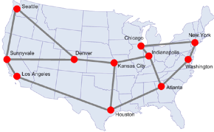
Refer to caption

Figure 5: Internet-2 network topology graph.

VI-B Real network data tests

Internet-2 network example. Real data including OD flow traffic levels are collected from the operation of the Internet-2 network (Internet backbone network across USA) [1], shown in Fig. 5. Flow traffic levels are recorded every 555-minute intervals, for a three-week operational period of Internet-2 during Dec. 8–28, 2008 [1]. Internet-2 comprises N=11𝑁11N=11 nodes, L=41𝐿41L=41 links, and F=121𝐹121F=121 flows. Given the OD flow traffic measurements, the link loads in 𝐘𝐘{\bf Y} are obtained through multiplication with the Internet-2 routing matrix, which in this case remains invariant during the three weeks of data acquisition [1]. Even though 𝐘𝐘{\bf Y} is “constructed” here from flow measurements, link loads can be typically acquired from SNMP traces [35].

The available OD flows are incomplete due to problems in the data collection process. In addition, flows can be modeled as the superposition of “clean” plus anomalous traffic, i.e., the sum of some unknown “ground-truth” low-rank and sparse matrices 𝒫Ω(𝐗0+𝐀0)subscript𝒫Ωsubscript𝐗0subscript𝐀0\mathcal{P}_{\Omega}({\bf X}_{0}+{\bf A}_{0}). Therefore, setting 𝐑=𝐈F𝐑subscript𝐈𝐹{\bf R}={\bf I}_{F} in (P1) one can first run the batch Algorithm 1 to estimate the “ground-truth” components {𝐗0,𝐀0}subscript𝐗0subscript𝐀0\{{\bf X}_{0},{\bf A}_{0}\}. The estimated 𝐗0subscript𝐗0{\bf X}_{0} exhibits three dominant singular values, confirming the low-rank property of the nominal traffic matrix. To be on the conservative side, only important spikes with magnitude greater than the threshold level 50𝐘F/LT50subscriptnorm𝐘𝐹𝐿𝑇50\|{\bf Y}\|_{F}/LT are retained as benchmark anomalies (nonzero entries in 𝐀0subscript𝐀0{\bf A}_{0}).

Comparison with PCA-based batch estimators [20][40]. To highlight the merits of the batch estimator (P3), its performance is compared with the spatial PCA-based schemes reported in [20] and [40]. These methods capitalize on the fact that the anomaly-free traffic matrix has low-rank, while the presence of anomalies considerably increases the rank of 𝐘𝐘{\bf Y}. Both algorithms rely on a two-step estimation procedure: (s1) perform PCA on the data 𝐘𝐘{\bf Y} to extract the (low-rank) anomaly-free link traffic matrix 𝐗~~𝐗\tilde{{\bf X}}; and (s2) declare anomalies based on the residual traffic 𝐘~:=𝐘𝐗~assign~𝐘𝐘~𝐗\tilde{{\bf Y}}:={\bf Y}-\tilde{{\bf X}}. The algorithms in [40] and [20] differ in the way (s2) is performed. On its operational phase, the algorithm in [20] declares the presence of an anomaly at time t𝑡t, when the projection of 𝐲tsubscript𝐲𝑡{\bf y}_{t} onto the anomalous subspace exceeds a prescribed threshold. It is clear that the aforementioned method is unable to identify anomalous flows. On the other hand, the network anomography approach of [40] capitalizes on the sparsity of anomalies, and recovers the anomaly matrix by minimizing 𝐀~1subscriptnorm~𝐀1\|\tilde{{\bf A}}\|_{1}, subject to the linear constraints 𝐘~=𝐑𝐀~~𝐘𝐑~𝐀\tilde{{\bf Y}}={\bf R}\tilde{{\bf A}}.

Refer to caption Refer to caption
(a) (b)
Figure 6: Performance of the batch estimator for Internet-2 network data. (a) ROC curves of the proposed versus the PCA-based methods. (b) Amplitude of the true (blue) and estimated (red) anomalies for PFA=0.04subscript𝑃FA0.04P_{\rm FA}=0.04 and PD=0.93subscript𝑃D0.93P_{\rm D}=0.93.

The aforementioned methods require a priori knowledge on the rank of the anomaly-free traffic matrix, and assume there is no missing data. To carry out performance comparisons, the detection rate will be adopted as figure of merit, which measures the algorithm’s success in identifying anomalies across both flows and time instants. ROC curves are depicted in Fig. 6 (a), for different values of the rank required to run the PCA-based methods. It is apparent that the estimator (P3) obtained via Algorithm 1 markedly outperforms both PCA-based methods in terms of detection performance. This is somehow expected, since (P3) advocates joint estimation of the anomalies and the nominal traffic matrix. For an instance of PFA=0.04subscript𝑃FA0.04P_{\rm FA}=0.04 and PD=0.93subscript𝑃D0.93P_{\rm D}=0.93, Fig. 6 (b) illustrates the effectiveness of the proposed algorithm in terms of unveiling the anomalous flows and time instants.
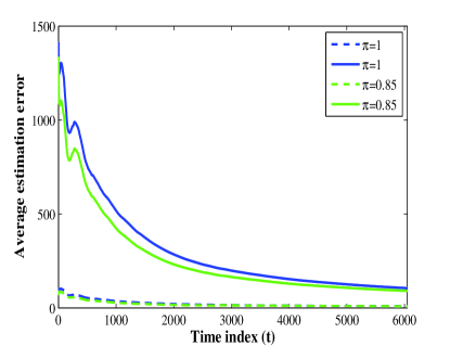
Refer to caption Refer to caption
(a) (b)
Refer to caption Refer to caption
(c) (d)
Figure 7: Performance of the online estimator for Internet-2 network data. (a) Evolution of average anomaly (dotted) and traffic (solid) estimation errors. (b) Evolution of average detection (solid) and false alarm (dotted) rates. (c) Estimated (red) versus true (blue) link traffic for thee representative links. (d) Estimated (circle markers) versus true (solid) anomalies for three representative flows when π=0.85𝜋0.85\pi=0.85.

Online operation. Algorithm 2 is tested here with the Internet-2 network data under two scenarios: with and without missing data. For the incomplete data case, a randomly chosen subset of link counts with cardinality 0.15×LT0.15𝐿𝑇0.15\times LT is discarded. The penalty parameters are tuned as λ1=0.7subscript𝜆10.7\lambda_{1}=0.7 and λ=1.4subscript𝜆1.4\lambda_{*}=1.4. The evolution of the average anomaly and traffic estimation errors, and average detection and false alarm rates are depicted in Fig. 7 (a), (b), respectively. Note how in the case of full-data, after about a week the traffic subspace is accurately learned and the detection (false alarm) rates approach the values 0.720.720.72 (0.0110.0110.011). It is further observed that even with 15%percent1515\% missing data, the detection performance degrades gracefully. Finally, Fig. 7(c)[(d)] depicts how three representative link traffic levels [OD flow anomalies] are accurately tracked over time.

VII Concluding remarks

An online algorithm is developed in this paper to perform a critical network monitoring task termed dynamic anomalography, meaning to unveil traffic volume anomalies in backbone networks adaptively. Given link-level traffic measurements (noisy superpositions of OD flows) acquired sequentially in time, the goal is to construct a map of anomalies in real time, that summarizes the network ‘health state’ along both the flow and time dimensions. Online algorithms enable tracking of anomalies in nonstationary environments, typically arising due to to e.g., routing changes and missing data. The resultant online schemes offer an attractive alternative to batch algorithms, since they scale gracefully as the number of flows in the network grows, or, the time window of data acquisition increases. Comprehensive numerical tests with both synthetic and real network data corroborate the effectiveness of the proposed algorithms and their tracking capabilities, and show that they outperform existing workhorse approaches for network anomaly detection.

A. Proof of Lemma IV-C: With 𝐏1,𝐏2subscript𝐏1subscript𝐏2{\bf P}_{1},{\bf P}_{2}\in\mathcal{L} consider the function

ut(𝐚,𝐏1,𝐏2):=12𝐅t(𝐏1)(𝐲t𝐑t𝐚)2212𝐅t(𝐏2)(𝐲t𝐑t𝐚)22assignsubscript𝑢𝑡𝐚subscript𝐏1subscript𝐏212superscriptsubscriptnormsubscript𝐅𝑡subscript𝐏1subscript𝐲𝑡subscript𝐑𝑡𝐚2212superscriptsubscriptnormsubscript𝐅𝑡subscript𝐏2subscript𝐲𝑡subscript𝐑𝑡𝐚22\displaystyle u_{t}({\bf a},{\bf P}_{1},{\bf P}_{2}):=\frac{1}{2}\|{\bf F}_{t}({\bf P}_{1})({\bf y}_{t}-{\bf R}_{t}{\bf a})\|_{2}^{2}-\frac{1}{2}\|{\bf F}_{t}({\bf P}_{2})({\bf y}_{t}-{\bf R}_{t}{\bf a})\|_{2}^{2} (23)

where 𝐅t(𝐏):=[𝛀t[𝐈L𝐏𝐃t(𝐏)]𝛀t,λ𝛀t𝐃t(𝐏)]assignsubscript𝐅𝑡𝐏superscriptsubscript𝛀𝑡delimited-[]subscript𝐈𝐿subscript𝐏𝐃𝑡𝐏subscript𝛀𝑡subscript𝜆subscript𝛀𝑡subscriptsuperscript𝐃𝑡𝐏{\bf F}_{t}({\bf P}):=\left[\mathbf{\Omega}_{t}\left[{\bf I}_{L}-{\bf P}{\bf D}_{t}({\bf P})\right]\mathbf{\Omega}_{t},~{}\sqrt{\lambda_{\ast}}\mathbf{\Omega}_{t}{\bf D}^{\prime}_{t}({\bf P})\right]^{\prime}, and 𝐃t(𝐏):=(λ𝐈ρ+𝐏𝛀t𝐏)1𝐏assignsubscript𝐃𝑡𝐏superscriptsubscript𝜆subscript𝐈𝜌superscript𝐏subscript𝛀𝑡𝐏1superscript𝐏{\bf D}_{t}({\bf P}):=\left(\lambda_{\ast}{\bf I}_{\rho}+{\bf P}^{\prime}\mathbf{\Omega}_{t}{\bf P}\right)^{-1}{\bf P}^{\prime}. It can be readily inferred from a5) that

ut(𝐚t(𝐏2),𝐏1,𝐏2)ut(𝐚t(𝐏1),𝐏1,𝐏2)c0𝐚t(𝐏2)𝐚t(𝐏1)22subscript𝑢𝑡subscript𝐚𝑡subscript𝐏2subscript𝐏1subscript𝐏2subscript𝑢𝑡subscript𝐚𝑡subscript𝐏1subscript𝐏1subscript𝐏2subscript𝑐0superscriptsubscriptnormsubscript𝐚𝑡subscript𝐏2subscript𝐚𝑡subscript𝐏122\displaystyle u_{t}({\bf a}_{t}({\bf P}_{2}),{\bf P}_{1},{\bf P}_{2})-u_{t}({\bf a}_{t}({\bf P}_{1}),{\bf P}_{1},{\bf P}_{2})\geq c_{0}\|{\bf a}_{t}({\bf P}_{2})-{\bf a}_{t}({\bf P}_{1})\|_{2}^{2} (24)

for some positive constant c0subscript𝑐0c_{0}. The rest of the proof deals with Lipschitz continuity of ut(.,𝐏1,𝐏2)u_{t}(.,{\bf P}_{1},{\bf P}_{2}). For 𝐚1subscript𝐚1{\bf a}_{1} and 𝐚2subscript𝐚2{\bf a}_{2} from a compact set 𝒜𝒜\mathcal{A}, consider

2|ut(𝐚1,𝐏1,𝐏2)ut(𝐚2,𝐏1,𝐏2)|=2subscript𝑢𝑡subscript𝐚1subscript𝐏1subscript𝐏2subscript𝑢𝑡subscript𝐚2subscript𝐏1subscript𝐏2absent\displaystyle 2|u_{t}({\bf a}_{1},{\bf P}_{1},{\bf P}_{2})-u_{t}({\bf a}_{2},{\bf P}_{1},{\bf P}_{2})|={} 2𝐑t[𝐅t(𝐏2)𝐅t(𝐏2)𝐅t(𝐏1)𝐅t(𝐏1)],(𝐚2𝐚1)𝐲t2subscriptsuperscript𝐑𝑡delimited-[]subscriptsuperscript𝐅𝑡subscript𝐏2subscript𝐅𝑡subscript𝐏2subscriptsuperscript𝐅𝑡subscript𝐏1subscript𝐅𝑡subscript𝐏1subscript𝐚2subscript𝐚1subscriptsuperscript𝐲𝑡\displaystyle 2\langle{\bf R}^{\prime}_{t}\left[{\bf F}^{\prime}_{t}({\bf P}_{2}){\bf F}_{t}({\bf P}_{2})-{\bf F}^{\prime}_{t}({\bf P}_{1}){\bf F}_{t}({\bf P}_{1})\right],({\bf a}_{2}-{\bf a}_{1}){\bf y}^{\prime}_{t}\rangle
+(𝐅t(𝐏1)𝐑t𝐚122𝐅t(𝐏1)𝐑t𝐚222)(𝐅t(𝐏2)𝐑t𝐚122𝐅t(𝐏2)𝐑t𝐚222).superscriptsubscriptnormsubscript𝐅𝑡subscript𝐏1subscript𝐑𝑡subscript𝐚122superscriptsubscriptnormsubscript𝐅𝑡subscript𝐏1subscript𝐑𝑡subscript𝐚222superscriptsubscriptnormsubscript𝐅𝑡subscript𝐏2subscript𝐑𝑡subscript𝐚122superscriptsubscriptnormsubscript𝐅𝑡subscript𝐏2subscript𝐑𝑡subscript𝐚222\displaystyle+\left(\|{\bf F}_{t}({\bf P}_{1}){\bf R}_{t}{\bf a}_{1}\|_{2}^{2}-\|{\bf F}_{t}({\bf P}_{1}){\bf R}_{t}{\bf a}_{2}\|_{2}^{2}\right)-\left(\|{\bf F}_{t}({\bf P}_{2}){\bf R}_{t}{\bf a}_{1}\|_{2}^{2}-\|{\bf F}_{t}({\bf P}_{2}){\bf R}_{t}{\bf a}_{2}\|_{2}^{2}\right). (25)

Introducing the auxiliary variable 𝚫a:=𝐚2𝐚1assignsubscript𝚫𝑎subscript𝐚2subscript𝐚1\bm{\Delta}_{a}:={\bf a}_{2}-{\bf a}_{1}, the last two summands in (25) can be bounded as

𝐅t(𝐏1)𝐑t𝐚122superscriptsubscriptnormsubscript𝐅𝑡subscript𝐏1subscript𝐑𝑡subscript𝐚122\displaystyle\|{\bf F}_{t}({\bf P}_{1}){\bf R}_{t}{\bf a}_{1}\|_{2}^{2} 𝐅t(𝐏1)𝐑t𝐚222𝐅t(𝐏2)𝐑t𝐚122+𝐅t(𝐏2)𝐑t𝐚222superscriptsubscriptnormsubscript𝐅𝑡subscript𝐏1subscript𝐑𝑡subscript𝐚222superscriptsubscriptnormsubscript𝐅𝑡subscript𝐏2subscript𝐑𝑡subscript𝐚122superscriptsubscriptnormsubscript𝐅𝑡subscript𝐏2subscript𝐑𝑡subscript𝐚222\displaystyle-\|{\bf F}_{t}({\bf P}_{1}){\bf R}_{t}{\bf a}_{2}\|_{2}^{2}-\|{\bf F}_{t}({\bf P}_{2}){\bf R}_{t}{\bf a}_{1}\|_{2}^{2}+\|{\bf F}_{t}({\bf P}_{2}){\bf R}_{t}{\bf a}_{2}\|_{2}^{2}
=(𝐅t(𝐏1)𝐑t𝚫a22𝐅t(𝐏2)𝐑t𝚫a22)+2𝐑t[𝐅t(𝐏2)𝐅t(𝐏2)𝐅t(𝐏1)𝐅t(𝐏1)],𝐚2𝚫aabsentsuperscriptsubscriptnormsubscript𝐅𝑡subscript𝐏1subscript𝐑𝑡subscript𝚫𝑎22superscriptsubscriptnormsubscript𝐅𝑡subscript𝐏2subscript𝐑𝑡subscript𝚫𝑎222subscriptsuperscript𝐑𝑡delimited-[]subscriptsuperscript𝐅𝑡subscript𝐏2subscript𝐅𝑡subscript𝐏2subscriptsuperscript𝐅𝑡subscript𝐏1subscript𝐅𝑡subscript𝐏1subscript𝐚2subscriptsuperscript𝚫𝑎\displaystyle=\left(\|{\bf F}_{t}({\bf P}_{1}){\bf R}_{t}\mathbf{\Delta}_{a}\|_{2}^{2}-\|{\bf F}_{t}({\bf P}_{2}){\bf R}_{t}\mathbf{\Delta}_{a}\|_{2}^{2}\right)+2\langle{\bf R}^{\prime}_{t}\left[{\bf F}^{\prime}_{t}({\bf P}_{2}){\bf F}_{t}({\bf P}_{2})-{\bf F}^{\prime}_{t}({\bf P}_{1}){\bf F}_{t}({\bf P}_{1})\right],{\bf a}_{2}\mathbf{\Delta}^{\prime}_{a}\ \rangle
c1𝐅t(𝐏2)𝐅t(𝐏1)𝚫a22+c2𝐅t(𝐏2)𝐅t(𝐏2)𝐅t(𝐏1)𝐅t(𝐏1)𝚫a2absentsubscript𝑐1normsubscript𝐅𝑡subscript𝐏2subscript𝐅𝑡subscript𝐏1superscriptsubscriptnormsubscript𝚫𝑎22subscript𝑐2normsubscriptsuperscript𝐅𝑡subscript𝐏2subscript𝐅𝑡subscript𝐏2subscriptsuperscript𝐅𝑡subscript𝐏1subscript𝐅𝑡subscript𝐏1subscriptnormsubscript𝚫𝑎2\displaystyle\leq c_{1}\|{\bf F}_{t}({\bf P}_{2})-{\bf F}_{t}({\bf P}_{1})\|\|\mathbf{\Delta}_{a}\|_{2}^{2}+c_{2}\|{\bf F}^{\prime}_{t}({\bf P}_{2}){\bf F}_{t}({\bf P}_{2})-{\bf F}^{\prime}_{t}({\bf P}_{1}){\bf F}_{t}({\bf P}_{1})\|\|\mathbf{\Delta}_{a}\|_{2}
c3𝐅t(𝐏2)𝐅t(𝐏1)𝚫a2absentsubscript𝑐3normsubscript𝐅𝑡subscript𝐏2subscript𝐅𝑡subscript𝐏1subscriptnormsubscript𝚫𝑎2\displaystyle\leq c_{3}\|{\bf F}_{t}({\bf P}_{2})-{\bf F}_{t}({\bf P}_{1})\|\|\mathbf{\Delta}_{a}\|_{2} (26)

for some constants c1,c2,c3>0subscript𝑐1subscript𝑐2subscript𝑐30c_{1},c_{2},c_{3}>0, since 𝐅t(𝐏)normsubscript𝐅𝑡𝐏\|{\bf F}_{t}({\bf P})\| for 𝐏𝐏{\bf P}\in\mathcal{L}, 𝚫a2subscriptnormsubscript𝚫𝑎2\|\mathbf{\Delta}_{a}\|_{2}, 𝐚22subscriptnormsubscript𝐚22\|{\bf a}_{2}\|_{2} for 𝐚1,𝐚2𝒜subscript𝐚1subscript𝐚2𝒜{\bf a}_{1},{\bf a}_{2}\in\mathcal{A}, and 𝐑tnormsubscript𝐑𝑡\|{\bf R}_{t}\| are all uniformly bounded. The first summand on the right-hand side of (25) is similarly bounded (details omitted here). Next, to establish that 𝐅t(𝐏)subscript𝐅𝑡𝐏{\bf F}_{t}({\bf P}) is Lipschitz one can derive the following bound (𝚫L:=𝐏2𝐏1assignsubscript𝚫𝐿subscript𝐏2subscript𝐏1\mathbf{\Delta}_{L}:={\bf P}_{2}-{\bf P}_{1})

𝐅t(𝐏2)𝐅t(𝐏1)normsubscript𝐅𝑡subscript𝐏2subscript𝐅𝑡subscript𝐏1\displaystyle\|{\bf F}_{t}({\bf P}_{2})-{\bf F}_{t}({\bf P}_{1})\| 𝛀t[𝐏2𝐃t(𝐏2)𝐏1𝐃t(𝐏1)]𝛀t+λ𝛀t(𝐃t(𝐏2)𝐃t(𝐏1))absentnormsubscript𝛀𝑡delimited-[]subscript𝐏2subscript𝐃𝑡subscript𝐏2subscript𝐏1subscript𝐃𝑡subscript𝐏1subscript𝛀𝑡subscript𝜆normsubscript𝛀𝑡subscriptsuperscript𝐃𝑡subscript𝐏2subscriptsuperscript𝐃𝑡subscript𝐏1\displaystyle\leq\|\mathbf{\Omega}_{t}\left[{\bf P}_{2}{\bf D}_{t}({\bf P}_{2})-{\bf P}_{1}{\bf D}_{t}({\bf P}_{1})\right]\mathbf{\Omega}_{t}\|+\sqrt{\lambda_{\ast}}\|\mathbf{\Omega}_{t}({\bf D}^{\prime}_{t}({\bf P}_{2})-{\bf D}^{\prime}_{t}({\bf P}_{1}))\|
𝐏1(𝐏1+λ)(λ𝐈ρ+𝐏2𝛀t𝐏2)1(λ𝐈ρ+𝐏1𝛀t𝐏1)1absentnormsubscript𝐏1normsubscript𝐏1subscript𝜆normsuperscriptsubscript𝜆subscript𝐈𝜌subscriptsuperscript𝐏2subscript𝛀𝑡subscript𝐏21superscriptsubscript𝜆subscript𝐈𝜌subscriptsuperscript𝐏1subscript𝛀𝑡subscript𝐏11\displaystyle\leq\|{\bf P}_{1}\|(\|{\bf P}_{1}\|+\sqrt{\lambda_{\ast}})\|(\lambda_{\ast}{\bf I}_{\rho}+{\bf P}^{\prime}_{2}\mathbf{\Omega}_{t}{\bf P}_{2})^{-1}-(\lambda_{\ast}{\bf I}_{\rho}+{\bf P}^{\prime}_{1}\mathbf{\Omega}_{t}{\bf P}_{1})^{-1}\|
+𝚫L(𝐏1+𝐏2+λ)(λ𝐈ρ+𝐏2𝛀t𝐏2)1.normsubscript𝚫𝐿normsubscript𝐏1normsubscript𝐏2subscript𝜆normsuperscriptsubscript𝜆subscript𝐈𝜌subscriptsuperscript𝐏2subscript𝛀𝑡subscript𝐏21\displaystyle\hskip 42.67912pt+\|\mathbf{\Delta}_{L}\|(\|{\bf P}_{1}\|+\|{\bf P}_{2}\|+\sqrt{\lambda_{\ast}})\|(\lambda_{\ast}{\bf I}_{\rho}+{\bf P}^{\prime}_{2}\mathbf{\Omega}_{t}{\bf P}_{2})^{-1}\|. (27)

Upon introducing 𝐆t𝐆t:=𝚫L𝛀t𝐏1+𝚫L𝛀t𝚫L+𝐏1𝛀t𝚫Lassignsubscriptsuperscript𝐆𝑡subscript𝐆𝑡subscriptsuperscript𝚫𝐿subscript𝛀𝑡subscript𝐏1subscriptsuperscript𝚫𝐿subscript𝛀𝑡subscript𝚫𝐿subscriptsuperscript𝐏1subscript𝛀𝑡subscript𝚫𝐿{\bf G}^{\prime}_{t}{\bf G}_{t}:=\mathbf{\Delta}^{\prime}_{L}\mathbf{\Omega}_{t}{\bf P}_{1}+\mathbf{\Delta}^{\prime}_{L}\mathbf{\Omega}_{t}\mathbf{\Delta}_{L}+{\bf P}^{\prime}_{1}\mathbf{\Omega}_{t}\mathbf{\Delta}_{L} and 𝐇t:=λ𝐈ρ+𝐏𝛀t𝐏assignsubscript𝐇𝑡subscript𝜆subscript𝐈𝜌𝐏subscript𝛀𝑡superscript𝐏{\bf H}_{t}:=\lambda_{\ast}{\bf I}_{\rho}+{\bf P}\mathbf{\Omega}_{t}{\bf P}^{\prime} by utilizing the matrix inversion lemma, the first term is bounded as follows

(λ𝐈ρ+𝐏2𝛀t𝐏2)1(λ𝐈ρ+𝐏1𝛀t𝐏1)1=normsuperscriptsubscript𝜆subscript𝐈𝜌subscriptsuperscript𝐏2subscript𝛀𝑡subscript𝐏21superscriptsubscript𝜆subscript𝐈𝜌subscriptsuperscript𝐏1subscript𝛀𝑡subscript𝐏11absent\displaystyle\|(\lambda_{\ast}{\bf I}_{\rho}+{\bf P}^{\prime}_{2}\mathbf{\Omega}_{t}{\bf P}_{2})^{-1}-(\lambda_{\ast}{\bf I}_{\rho}+{\bf P}^{\prime}_{1}\mathbf{\Omega}_{t}{\bf P}_{1})^{-1}\|={} 𝐇t1(𝐏1)𝐆t(𝐈+𝐆t𝐇t1(𝐏1)𝐆t)1𝐆t𝐇t1(𝐏1)normsuperscriptsubscript𝐇𝑡1subscript𝐏1subscript𝐆𝑡superscript𝐈subscriptsuperscript𝐆𝑡superscriptsubscript𝐇𝑡1subscript𝐏1subscript𝐆𝑡1subscriptsuperscript𝐆𝑡superscriptsubscript𝐇𝑡1subscript𝐏1\displaystyle\|{\bf H}_{t}^{-1}({\bf P}_{1}){\bf G}_{t}({\bf I}+{\bf G}^{\prime}_{t}{\bf H}_{t}^{-1}({\bf P}_{1}){\bf G}_{t})^{-1}{\bf G}^{\prime}_{t}{\bf H}_{t}^{-1}({\bf P}_{1})\|
\displaystyle\leq{} 𝐇t1(𝐏1)2𝐆t2(𝐈+𝐆t𝐇t1(𝐏1)𝐆t)1superscriptnormsuperscriptsubscript𝐇𝑡1subscript𝐏12superscriptnormsubscript𝐆𝑡2normsuperscript𝐈subscriptsuperscript𝐆𝑡superscriptsubscript𝐇𝑡1subscript𝐏1subscript𝐆𝑡1\displaystyle\|{\bf H}_{t}^{-1}({\bf P}_{1})\|^{2}\|{\bf G}_{t}\|^{2}\|({\bf I}+{\bf G}^{\prime}_{t}{\bf H}_{t}^{-1}({\bf P}_{1}){\bf G}_{t})^{-1}\|
\displaystyle\leq{} (1λ)2𝐆t2c4𝚫L.superscript1subscript𝜆2superscriptnormsubscript𝐆𝑡2subscript𝑐4normsubscript𝚫𝐿\displaystyle\left(\frac{1}{\lambda_{\ast}}\right)^{2}\|{\bf G}_{t}\|^{2}\leq c_{4}\|\mathbf{\Delta}_{L}\|. (28)

Putting the pieces together 𝐅t(.){\bf F}_{t}(.) is found to be Lipschitz and subsequently (25) is bounded by a constant factor of 𝚫L𝚫a2normsubscript𝚫𝐿subscriptnormsubscript𝚫𝑎2\|\mathbf{\Delta}_{L}\|\|\mathbf{\Delta}_{a}\|_{2}. Substituting 𝐚1=𝐚t(𝐏1)subscript𝐚1subscript𝐚𝑡subscript𝐏1{\bf a}_{1}={\bf a}_{t}({\bf P}_{1}) and 𝐚2=𝐚t(𝐏2)subscript𝐚2subscript𝐚𝑡subscript𝐏2{\bf a}_{2}={\bf a}_{t}({\bf P}_{2}) along with the bound in (24) yields the desired result 𝐚t(𝐏2)𝐚t(𝐏1)2c5𝐏2𝐏1subscriptnormsubscript𝐚𝑡subscript𝐏2subscript𝐚𝑡subscript𝐏12subscript𝑐5normsubscript𝐏2subscript𝐏1\|{\bf a}_{t}({\bf P}_{2})-{\bf a}_{t}({\bf P}_{1})\|_{2}\leq c_{5}\|{\bf P}_{2}-{\bf P}_{1}\|. Furthermore, from the relationship 𝐪t=𝐃t(𝐏)𝛀t(𝐲t𝐑t𝐚t)subscript𝐪𝑡subscript𝐃𝑡𝐏subscript𝛀𝑡subscript𝐲𝑡subscript𝐑𝑡subscript𝐚𝑡{\bf q}_{t}={\bf D}_{t}({\bf P})\mathbf{\Omega}_{t}({\bf y}_{t}-{\bf R}_{t}{\bf a}_{t}), Lipschitz continuity of 𝐪t(𝐏)subscript𝐪𝑡𝐏{\bf q}_{t}({\bf P}) readily follows.

Moreover, gt(𝐏,𝐪[t],𝐚[t])subscript𝑔𝑡𝐏𝐪delimited-[]𝑡𝐚delimited-[]𝑡g_{t}({\bf P},{\bf q}[t],{\bf a}[t]) is a quadratic function on a compact set, and thus clearly Lipschitz continuous. To prove Lipschitz continuity of t(𝐏)subscript𝑡𝐏\ell_{t}({\bf P}), recall the definition {𝐪t(𝐏),𝐚t(𝐏)}=argmin{𝐪,𝐚}gt(𝐏,𝐪,𝐚)subscript𝐪𝑡𝐏subscript𝐚𝑡𝐏subscript𝐪𝐚subscript𝑔𝑡𝐏𝐪𝐚\{{\bf q}_{t}({\bf P}),{\bf a}_{t}({\bf P})\}=\arg\min_{\{{\bf q},{\bf a}\}}g_{t}({\bf P},{\bf q},{\bf a}) to obtain after some algebra

t(𝐏2)t(𝐏1)=subscript𝑡subscript𝐏2subscript𝑡subscript𝐏1absent\displaystyle\ell_{t}({\bf P}_{2})-\ell_{t}({\bf P}_{1})={} 12𝒫Ωt(𝐏2𝐪t(𝐏2)+𝐑t𝐚t(𝐏2))22𝒫Ωt(𝐏1𝐪t(𝐏1)+𝐑t𝐚t(𝐏1))2212superscriptsubscriptnormsubscript𝒫subscriptΩ𝑡subscript𝐏2subscript𝐪𝑡subscript𝐏2subscript𝐑𝑡subscript𝐚𝑡subscript𝐏222superscriptsubscriptnormsubscript𝒫subscriptΩ𝑡subscript𝐏1subscript𝐪𝑡subscript𝐏1subscript𝐑𝑡subscript𝐚𝑡subscript𝐏122\displaystyle\frac{1}{2}\|\mathcal{P}_{\Omega_{t}}({\bf P}_{2}{\bf q}_{t}({\bf P}_{2})+{\bf R}_{t}{\bf a}_{t}({\bf P}_{2}))\|_{2}^{2}-\|\mathcal{P}_{\Omega_{t}}({\bf P}_{1}{\bf q}_{t}({\bf P}_{1})+{\bf R}_{t}{\bf a}_{t}({\bf P}_{1}))\|_{2}^{2}
𝒫Ωt(𝐲t),𝐏2𝐪t(𝐏2)+𝐑t𝐚t(𝐏2)𝐏1𝐪t(𝐏1)𝐑t𝐚t(𝐏1)subscript𝒫subscriptΩ𝑡subscript𝐲𝑡subscript𝐏2subscript𝐪𝑡subscript𝐏2subscript𝐑𝑡subscript𝐚𝑡subscript𝐏2subscript𝐏1subscript𝐪𝑡subscript𝐏1subscript𝐑𝑡subscript𝐚𝑡subscript𝐏1\displaystyle-\langle\mathcal{P}_{\Omega_{t}}({\bf y}_{t}),{\bf P}_{2}{\bf q}_{t}({\bf P}_{2})+{\bf R}_{t}{\bf a}_{t}({\bf P}_{2})-{\bf P}_{1}{\bf q}_{t}({\bf P}_{1})-{\bf R}_{t}{\bf a}_{t}({\bf P}_{1})\rangle
+λ2(𝐪t(𝐏2)22𝐪t(𝐏1)22)+λ1(𝐚t(𝐏2)1𝐚t(𝐏1)1).subscript𝜆2superscriptsubscriptnormsubscript𝐪𝑡subscript𝐏222superscriptsubscriptnormsubscript𝐪𝑡subscript𝐏122subscript𝜆1subscriptnormsubscript𝐚𝑡subscript𝐏21subscriptnormsubscript𝐚𝑡subscript𝐏11\displaystyle+\frac{\lambda_{\ast}}{2}\big{(}\|{\bf q}_{t}({\bf P}_{2})\|_{2}^{2}-\|{\bf q}_{t}({\bf P}_{1})\|_{2}^{2}\big{)}+\lambda_{1}\big{(}\|{\bf a}_{t}({\bf P}_{2})\|_{1}-\|{\bf a}_{t}({\bf P}_{1})\|_{1}\big{)}. (29)

The first term in the right-hand side of (29) is bounded as

𝒫Ωt(𝐏2𝐪t(𝐏2)+𝐑t𝐚t(𝐏2))22𝒫Ωt(𝐏1𝐪t(𝐏1)+𝐑t𝐚t(𝐏1))22superscriptsubscriptnormsubscript𝒫subscriptΩ𝑡subscript𝐏2subscript𝐪𝑡subscript𝐏2subscript𝐑𝑡subscript𝐚𝑡subscript𝐏222superscriptsubscriptnormsubscript𝒫subscriptΩ𝑡subscript𝐏1subscript𝐪𝑡subscript𝐏1subscript𝐑𝑡subscript𝐚𝑡subscript𝐏122absent\displaystyle\|\mathcal{P}_{\Omega_{t}}({\bf P}_{2}{\bf q}_{t}({\bf P}_{2})+{\bf R}_{t}{\bf a}_{t}({\bf P}_{2}))\|_{2}^{2}-\|\mathcal{P}_{\Omega_{t}}({\bf P}_{1}{\bf q}_{t}({\bf P}_{1})+{\bf R}_{t}{\bf a}_{t}({\bf P}_{1}))\|_{2}^{2}\leq
(𝒫Ωt(𝐏2𝐪t(𝐏2)𝐏1𝐪t(𝐏1))2+𝒫Ωt(𝐑t𝐚t(𝐏2)𝐑t𝐚t(𝐏1))2)subscriptnormsubscript𝒫subscriptΩ𝑡subscript𝐏2subscript𝐪𝑡subscript𝐏2subscript𝐏1subscript𝐪𝑡subscript𝐏12subscriptnormsubscript𝒫subscriptΩ𝑡subscript𝐑𝑡subscript𝐚𝑡subscript𝐏2subscript𝐑𝑡subscript𝐚𝑡subscript𝐏12\displaystyle\hskip 79.66771pt\big{(}\|\mathcal{P}_{\Omega_{t}}({\bf P}_{2}{\bf q}_{t}({\bf P}_{2})-{\bf P}_{1}{\bf q}_{t}({\bf P}_{1}))\|_{2}+\|\mathcal{P}_{\Omega_{t}}({\bf R}_{t}{\bf a}_{t}({\bf P}_{2})-{\bf R}_{t}{\bf a}_{t}({\bf P}_{1}))\|_{2}\big{)}
×(𝒫Ωt(𝐏2𝐪t(𝐏2)+𝐑t𝐚t(𝐏2))2+𝒫Ωt(𝐏1𝐪t(𝐏1)+𝐑t𝐚t(𝐏1))2)absentsubscriptnormsubscript𝒫subscriptΩ𝑡subscript𝐏2subscript𝐪𝑡subscript𝐏2subscript𝐑𝑡subscript𝐚𝑡subscript𝐏22subscriptnormsubscript𝒫subscriptΩ𝑡subscript𝐏1subscript𝐪𝑡subscript𝐏1subscript𝐑𝑡subscript𝐚𝑡subscript𝐏12\displaystyle\hskip 79.66771pt\times\big{(}\|\mathcal{P}_{\Omega_{t}}({\bf P}_{2}{\bf q}_{t}({\bf P}_{2})+{\bf R}_{t}{\bf a}_{t}({\bf P}_{2}))\|_{2}+\|\mathcal{P}_{\Omega_{t}}({\bf P}_{1}{\bf q}_{t}({\bf P}_{1})+{\bf R}_{t}{\bf a}_{t}({\bf P}_{1}))\|_{2}\big{)}
c6(𝐏2𝐏1𝐪t(𝐏2)2+𝐏1𝐪t(𝐏2)𝐪t(𝐏1)2+𝐑t𝐚t(𝐏2)𝐚t(𝐏1)2)absentsubscript𝑐6normsubscript𝐏2subscript𝐏1subscriptnormsubscript𝐪𝑡subscript𝐏22normsubscript𝐏1subscriptnormsubscript𝐪𝑡subscript𝐏2subscript𝐪𝑡subscript𝐏12normsubscript𝐑𝑡subscriptnormsubscript𝐚𝑡subscript𝐏2subscript𝐚𝑡subscript𝐏12\displaystyle\hskip 79.66771pt\leq c_{6}\big{(}\|{\bf P}_{2}-{\bf P}_{1}\|\|{\bf q}_{t}({\bf P}_{2})\|_{2}+\|{\bf P}_{1}\|\|{\bf q}_{t}({\bf P}_{2})-{\bf q}_{t}({\bf P}_{1})\|_{2}+\|{\bf R}_{t}\|\|{\bf a}_{t}({\bf P}_{2})-{\bf a}_{t}({\bf P}_{1})\|_{2}\big{)} (30)

for some constant c6>0subscript𝑐60c_{6}>0. The second one is bounded as

𝒫Ωt(𝐲t),𝐏2𝐪t(𝐏2)+𝐑t𝐚t(𝐏2)𝐏1𝐪t(𝐏1)𝐑t𝐚t(𝐏1)subscript𝒫subscriptΩ𝑡subscript𝐲𝑡subscript𝐏2subscript𝐪𝑡subscript𝐏2subscript𝐑𝑡subscript𝐚𝑡subscript𝐏2subscript𝐏1subscript𝐪𝑡subscript𝐏1subscript𝐑𝑡subscript𝐚𝑡subscript𝐏1\displaystyle\langle\mathcal{P}_{\Omega_{t}}({\bf y}_{t}),{\bf P}_{2}{\bf q}_{t}({\bf P}_{2})+{\bf R}_{t}{\bf a}_{t}({\bf P}_{2})-{\bf P}_{1}{\bf q}_{t}({\bf P}_{1})-{\bf R}_{t}{\bf a}_{t}({\bf P}_{1})\rangle
𝒫Ωt(𝐲t)2(𝒫Ωt(𝐏2𝐪t(𝐏2)𝐏1𝐪t(𝐏1))2+𝒫Ωt(𝐑t𝐚t(𝐏2)𝐑t𝐚t(𝐏1))2)absentsubscriptnormsubscript𝒫subscriptΩ𝑡subscript𝐲𝑡2subscriptnormsubscript𝒫subscriptΩ𝑡subscript𝐏2subscript𝐪𝑡subscript𝐏2subscript𝐏1subscript𝐪𝑡subscript𝐏12subscriptnormsubscript𝒫subscriptΩ𝑡subscript𝐑𝑡subscript𝐚𝑡subscript𝐏2subscript𝐑𝑡subscript𝐚𝑡subscript𝐏12\displaystyle\hskip 56.9055pt\leq\|\mathcal{P}_{\Omega_{t}}({\bf y}_{t})\|_{2}\big{(}\|\mathcal{P}_{\Omega_{t}}({\bf P}_{2}{\bf q}_{t}({\bf P}_{2})-{\bf P}_{1}{\bf q}_{t}({\bf P}_{1}))\|_{2}+\|\mathcal{P}_{\Omega_{t}}({\bf R}_{t}{\bf a}_{t}({\bf P}_{2})-{\bf R}_{t}{\bf a}_{t}({\bf P}_{1}))\|_{2}\big{)}
𝒫Ωt(𝐲t)2(𝐏2𝐏1𝐪t(𝐏2)2+𝐏1𝐪t(𝐏2)𝐪t(𝐏1)2+𝐑t𝐚t(𝐏2)𝐚t(𝐏1)2).absentsubscriptnormsubscript𝒫subscriptΩ𝑡subscript𝐲𝑡2normsubscript𝐏2subscript𝐏1subscriptnormsubscript𝐪𝑡subscript𝐏22normsubscript𝐏1subscriptnormsubscript𝐪𝑡subscript𝐏2subscript𝐪𝑡subscript𝐏12normsubscript𝐑𝑡subscriptnormsubscript𝐚𝑡subscript𝐏2subscript𝐚𝑡subscript𝐏12\displaystyle\hskip 56.9055pt\leq\|\mathcal{P}_{\Omega_{t}}({\bf y}_{t})\|_{2}\big{(}\|{\bf P}_{2}-{\bf P}_{1}\|\|{\bf q}_{t}({\bf P}_{2})\|_{2}+\|{\bf P}_{1}\|\|{\bf q}_{t}({\bf P}_{2})-{\bf q}_{t}({\bf P}_{1})\|_{2}+\|{\bf R}_{t}\|\|{\bf a}_{t}({\bf P}_{2})-{\bf a}_{t}({\bf P}_{1})\|_{2}\big{)}. (31)

Finally, one can bound the third term in (29) as

λ2(𝐪t(𝐏2)22𝐪t(𝐏1)22)+λ1(𝐚t(𝐏2)1𝐚t(𝐏1)1)subscript𝜆2superscriptsubscriptnormsubscript𝐪𝑡subscript𝐏222superscriptsubscriptnormsubscript𝐪𝑡subscript𝐏122subscript𝜆1subscriptnormsubscript𝐚𝑡subscript𝐏21subscriptnormsubscript𝐚𝑡subscript𝐏11absent\displaystyle\frac{\lambda_{\ast}}{2}\big{(}\|{\bf q}_{t}({\bf P}_{2})\|_{2}^{2}-\|{\bf q}_{t}({\bf P}_{1})\|_{2}^{2}\big{)}+\lambda_{1}\big{(}\|{\bf a}_{t}({\bf P}_{2})\|_{1}-\|{\bf a}_{t}({\bf P}_{1})\|_{1}\big{)}\leq
λ2𝐪t(𝐏2)𝐪t(𝐏1)2(𝐪t(𝐏2)2+𝐪t(𝐏1)2)+λ1F𝐚t(𝐏2)𝐚t(𝐏1)2.subscript𝜆2subscriptnormsubscript𝐪𝑡subscript𝐏2subscript𝐪𝑡subscript𝐏12subscriptnormsubscript𝐪𝑡subscript𝐏22subscriptnormsubscript𝐪𝑡subscript𝐏12subscript𝜆1𝐹subscriptnormsubscript𝐚𝑡subscript𝐏2subscript𝐚𝑡subscript𝐏12\displaystyle\hskip 85.35826pt\frac{\lambda_{\ast}}{2}\|{\bf q}_{t}({\bf P}_{2})-{\bf q}_{t}({\bf P}_{1})\|_{2}\big{(}\|{\bf q}_{t}({\bf P}_{2})\|_{2}+\|{\bf q}_{t}({\bf P}_{1})\|_{2}\big{)}+\lambda_{1}\sqrt{F}\|{\bf a}_{t}({\bf P}_{2})-{\bf a}_{t}({\bf P}_{1})\|_{2}. (32)

Since 𝐪t(𝐏)subscript𝐪𝑡𝐏{\bf q}_{t}({\bf P}) and 𝐚t(𝐏)subscript𝐚𝑡𝐏{\bf a}_{t}({\bf P}) are Lipschitz as proved earlier, and 𝐏1,𝐏2subscript𝐏1subscript𝐏2{\bf P}_{1},{\bf P}_{2}\in\mathcal{L} are uniformly bounded, the expressions in the right-hand side of (30)-(32) are upper bounded by a constant factor of 𝐏2𝐏1normsubscript𝐏2subscript𝐏1\|{\bf P}_{2}-{\bf P}_{1}\|, and so is |t(𝐏2)t(𝐏1)|subscript𝑡subscript𝐏2subscript𝑡subscript𝐏1|\ell_{t}({\bf P}_{2})-\ell_{t}({\bf P}_{1})| after applying the triangle inequality to (29).

Regarding t(𝐏)subscript𝑡𝐏\nabla\ell_{t}({\bf P}), notice first that since {𝐪t(𝐏),𝐚t(𝐏)}subscript𝐪𝑡𝐏subscript𝐚𝑡𝐏\{{\bf q}_{t}({\bf P}),{\bf a}_{t}({\bf P})\} is the unique minimizer of gt(𝐏,𝐪,𝐚)subscript𝑔𝑡𝐏𝐪𝐚g_{t}({\bf P},{\bf q},{\bf a}) [cf. a5)], Danskin’s theorem [6, Prop. B.25(a)] implies that t(𝐏)=𝒫Ωt(𝐲t𝐏𝐪t(𝐏)𝐑t𝐚t(𝐏))𝐪t(𝐏)subscript𝑡𝐏subscript𝒫subscriptΩ𝑡subscript𝐲𝑡subscript𝐏𝐪𝑡𝐏subscript𝐑𝑡subscript𝐚𝑡𝐏subscriptsuperscript𝐪𝑡𝐏\nabla\ell_{t}({\bf P})=\mathcal{P}_{{\Omega}_{t}}({\bf y}_{t}-{\bf P}{\bf q}_{t}({\bf P})-{\bf R}_{t}{\bf a}_{t}({\bf P})){\bf q}^{\prime}_{t}({\bf P}). In the sequel, the triangle inequality will be used to split the norm in the right-hand side of

t(𝐏2)t(𝐏1)F=subscriptnormsubscript𝑡subscript𝐏2subscript𝑡subscript𝐏1𝐹absent\displaystyle\big{\|}\nabla\ell_{t}({\bf P}_{2})-\nabla\ell_{t}({\bf P}_{1})\big{\|}_{F}= 𝒫Ωt(𝐲t)[𝐪t(𝐏2)𝐪t(𝐏1)][𝒫Ωt(𝐏2𝐪t(𝐏2))𝐪t(𝐏2)𝒫Ωt(𝐏1𝐪t(𝐏1))𝐪t(𝐏1)]\displaystyle\big{\|}\mathcal{P}_{\Omega_{t}}({\bf y}_{t})\left[{\bf q}_{t}({\bf P}_{2})-{\bf q}_{t}({\bf P}_{1})\right]^{\prime}-\left[\mathcal{P}_{\Omega_{t}}({\bf P}_{2}{\bf q}_{t}({\bf P}_{2})){\bf q}^{\prime}_{t}({\bf P}_{2})-\mathcal{P}_{\Omega_{t}}({\bf P}_{1}{\bf q}_{t}({\bf P}_{1})){\bf q}^{\prime}_{t}({\bf P}_{1})\right]
[𝒫Ωt(𝐑t𝐚t(𝐏2))𝐪t(𝐏2)𝒫Ωt(𝐑t𝐚t(𝐏1))𝐪t(𝐏1)]F.evaluated-atdelimited-[]subscript𝒫subscriptΩ𝑡subscript𝐑𝑡subscript𝐚𝑡subscript𝐏2subscriptsuperscript𝐪𝑡subscript𝐏2subscript𝒫subscriptΩ𝑡subscript𝐑𝑡subscript𝐚𝑡subscript𝐏1subscriptsuperscript𝐪𝑡subscript𝐏1𝐹\displaystyle-\left[\mathcal{P}_{\Omega_{t}}({\bf R}_{t}{\bf a}_{t}({\bf P}_{2})){\bf q}^{\prime}_{t}({\bf P}_{2})-\mathcal{P}_{\Omega_{t}}({\bf R}_{t}{\bf a}_{t}({\bf P}_{1})){\bf q}^{\prime}_{t}({\bf P}_{1})\right]\big{\|}_{F}. (33)

The first term inside the norm is bounded as

𝒫Ωt(𝐲t)[𝐪t(𝐏2)𝐪t(𝐏1)]F𝒫Ωt(𝐲t)2𝐪t(𝐏2)𝐪t(𝐏1)2.subscriptnormsubscript𝒫subscriptΩ𝑡subscript𝐲𝑡superscriptdelimited-[]subscript𝐪𝑡subscript𝐏2subscript𝐪𝑡subscript𝐏1𝐹subscriptnormsubscript𝒫subscriptΩ𝑡subscript𝐲𝑡2subscriptnormsubscript𝐪𝑡subscript𝐏2subscript𝐪𝑡subscript𝐏12\displaystyle\|\mathcal{P}_{\Omega_{t}}({\bf y}_{t})\left[{\bf q}_{t}({\bf P}_{2})-{\bf q}_{t}({\bf P}_{1})\right]^{\prime}\|_{F}\leq\|\mathcal{P}_{\Omega_{t}}({\bf y}_{t})\|_{2}\|{\bf q}_{t}({\bf P}_{2})-{\bf q}_{t}({\bf P}_{1})\|_{2}. (34)

After some algebraic manipulations, the second term is also bounded as

𝒫Ωt(𝐏2𝐪t(𝐏2))𝐪t(𝐏2)𝒫Ωt(𝐏1𝐪t(𝐏1))𝐪t(𝐏1)Fsubscriptnormsubscript𝒫subscriptΩ𝑡subscript𝐏2subscript𝐪𝑡subscript𝐏2subscriptsuperscript𝐪𝑡subscript𝐏2subscript𝒫subscriptΩ𝑡subscript𝐏1subscript𝐪𝑡subscript𝐏1subscriptsuperscript𝐪𝑡subscript𝐏1𝐹absent\displaystyle\|\mathcal{P}_{\Omega_{t}}({\bf P}_{2}{\bf q}_{t}({\bf P}_{2})){\bf q}^{\prime}_{t}({\bf P}_{2})-\mathcal{P}_{\Omega_{t}}({\bf P}_{1}{\bf q}_{t}({\bf P}_{1})){\bf q}^{\prime}_{t}({\bf P}_{1})\|_{F}\leq{} 𝐏2𝐏1F𝐪t(𝐏2)22subscriptnormsubscript𝐏2subscript𝐏1𝐹superscriptsubscriptnormsubscript𝐪𝑡subscript𝐏222\displaystyle\|{\bf P}_{2}-{\bf P}_{1}\|_{F}\|{\bf q}_{t}({\bf P}_{2})\|_{2}^{2}
+𝐪t(𝐏2)𝐪t(𝐏1)2(𝐪t(𝐏2)2+𝐪t(𝐏1)2)subscriptnormsubscript𝐪𝑡subscript𝐏2subscript𝐪𝑡subscript𝐏12subscriptnormsubscript𝐪𝑡subscript𝐏22subscriptnormsubscript𝐪𝑡subscript𝐏12\displaystyle+\|{\bf q}_{t}({\bf P}_{2})-{\bf q}_{t}({\bf P}_{1})\|_{2}\big{(}\|{\bf q}_{t}({\bf P}_{2})\|_{2}+\|{\bf q}_{t}({\bf P}_{1})\|_{2}\big{)} (35)

and finally one can simply bound the third term as

𝒫Ωt(𝐑t𝐚t(𝐏2))𝐪t(𝐏2)𝒫Ωt(𝐑t𝐚t(𝐏1))𝐪t(𝐏1)Fsubscriptnormsubscript𝒫subscriptΩ𝑡subscript𝐑𝑡subscript𝐚𝑡subscript𝐏2subscriptsuperscript𝐪𝑡subscript𝐏2subscript𝒫subscriptΩ𝑡subscript𝐑𝑡subscript𝐚𝑡subscript𝐏1subscriptsuperscript𝐪𝑡subscript𝐏1𝐹absent\displaystyle\|\mathcal{P}_{\Omega_{t}}({\bf R}_{t}{\bf a}_{t}({\bf P}_{2})){\bf q}^{\prime}_{t}({\bf P}_{2})-\mathcal{P}_{\Omega_{t}}({\bf R}_{t}{\bf a}_{t}({\bf P}_{1})){\bf q}^{\prime}_{t}({\bf P}_{1})\|_{F}\leq{} 𝐑t(𝐚t(𝐏2)𝐚t(𝐏1)2𝐪t(𝐏1)2\displaystyle\|{\bf R}_{t}\|\big{(}\|{\bf a}_{t}({\bf P}_{2})-{\bf a}_{t}({\bf P}_{1})\|_{2}\|{\bf q}_{t}({\bf P}_{1})\|_{2}
+𝐪t(𝐏2)𝐪t(𝐏1)2𝐚t(𝐏1)2).\displaystyle+\|{\bf q}_{t}({\bf P}_{2})-{\bf q}_{t}({\bf P}_{1})\|_{2}\|{\bf a}_{t}({\bf P}_{1})\|_{2}\big{)}. (36)

Since 𝐚t(𝐏)subscript𝐚𝑡𝐏{\bf a}_{t}({\bf P}) and 𝐪t(𝐏)subscript𝐪𝑡𝐏{\bf q}_{t}({\bf P}) are Lipschitz and uniformly bounded, from (34)-(36) one can easily deduce that t(.)\nabla\ell_{t}(.) is indeed Lipschitz continuous. \blacksquare

B. Proof of Lemma IV-C: Exploiting that C^t(𝐏[t])=C^t+1(𝐏[t+1])=𝟎L×ρsubscript^𝐶𝑡𝐏delimited-[]𝑡subscript^𝐶𝑡1𝐏delimited-[]𝑡1subscript0𝐿𝜌\nabla\hat{C}_{t}({\bf P}[t])=\nabla\hat{C}_{t+1}({\bf P}[t+1])=\mathbf{0}_{L\times\rho} by algorithmic construction and the strong convexity assumption on C^tsubscript^𝐶𝑡\hat{C}_{t} [cf. a4)], application of the mean-value theorem readily yields

C^t(𝐏[t+1])C^t(𝐏[t])+c2𝐏[t+1]𝐏[t]F2subscript^𝐶𝑡𝐏delimited-[]𝑡1subscript^𝐶𝑡𝐏delimited-[]𝑡𝑐2superscriptsubscriptnorm𝐏delimited-[]𝑡1𝐏delimited-[]𝑡𝐹2\displaystyle\hat{C}_{t}({\bf P}[t+1])\geq\hat{C}_{t}({\bf P}[t])+\frac{c}{2}\|{\bf P}[t+1]-{\bf P}[t]\|_{F}^{2}
C^t+1(𝐏[t])C^t+1(𝐏[t+1])+c2𝐏[t+1]𝐏[t]F2.subscript^𝐶𝑡1𝐏delimited-[]𝑡subscript^𝐶𝑡1𝐏delimited-[]𝑡1𝑐2superscriptsubscriptnorm𝐏delimited-[]𝑡1𝐏delimited-[]𝑡𝐹2\displaystyle\hat{C}_{t+1}({\bf P}[t])\geq\hat{C}_{t+1}({\bf P}[t+1])+\frac{c}{2}\|{\bf P}[t+1]-{\bf P}[t]\|_{F}^{2}.

Upon defining the function ht(𝐏):=C^t(𝐏)C^t+1(𝐏)assignsubscript𝑡𝐏subscript^𝐶𝑡𝐏subscript^𝐶𝑡1𝐏h_{t}({\bf P}):=\hat{C}_{t}({\bf P})-\hat{C}_{t+1}({\bf P}) one arrives at

c𝐏[t+1]𝐏[t]F2ht(𝐏[t+1])ht(𝐏[t]).𝑐superscriptsubscriptnorm𝐏delimited-[]𝑡1𝐏delimited-[]𝑡𝐹2subscript𝑡𝐏delimited-[]𝑡1subscript𝑡𝐏delimited-[]𝑡\displaystyle c\|{\bf P}[t+1]-{\bf P}[t]\|_{F}^{2}\leq h_{t}({\bf P}[t+1])-h_{t}({\bf P}[t]). (37)

To complete the proof, it suffices to show that htsubscript𝑡h_{t} is Lipschitz with constant 𝒪(1/t)𝒪1𝑡\mathcal{O}(1/t), and upper bound the right-hand side of (37) accordingly. Since [cf. (16)]

ht(𝐏)=1t(t+1)τ=1tgτ(𝐏,𝐪[τ],𝐚[τ])1t+1gt+1(𝐏,𝐪[t+1],𝐚[t+1])+λ2t(t+1)𝐏F2subscript𝑡𝐏1𝑡𝑡1superscriptsubscript𝜏1𝑡subscript𝑔𝜏𝐏𝐪delimited-[]𝜏𝐚delimited-[]𝜏1𝑡1subscript𝑔𝑡1𝐏𝐪delimited-[]𝑡1𝐚delimited-[]𝑡1subscript𝜆2𝑡𝑡1superscriptsubscriptnorm𝐏𝐹2h_{t}({\bf P})=\frac{1}{t(t+1)}\sum_{\tau=1}^{t}g_{\tau}({\bf P},{\bf q}[\tau],{\bf a}[\tau])-\frac{1}{t+1}g_{t+1}({\bf P},{\bf q}[t+1],{\bf a}[t+1])+\frac{\lambda_{\ast}}{2t(t+1)}\|{\bf P}\|_{F}^{2} (38)

and gi(𝐏)subscript𝑔𝑖𝐏g_{i}({\bf P}) is Lipschitz according to Lemma IV-C, it follows that htsubscript𝑡h_{t} is Lipschitz with constant 𝒪(1/t)𝒪1𝑡\mathcal{O}(1/t). \blacksquare

C. Proof of Lemma IV-C: The first step of the proof is to show that {C^t(𝐏[t])}t=1superscriptsubscriptsubscript^𝐶𝑡𝐏delimited-[]𝑡𝑡1\{\hat{C}_{t}({\bf P}[t])\}_{t=1}^{\infty} is a quasi-matringale sequence, and hence convergent a.s. [22]. Building on the variations of C^t(𝐏[t])subscript^𝐶𝑡𝐏delimited-[]𝑡\hat{C}_{t}({\bf P}[t]), one can write

C^t+1(𝐏[t+1])C^t(𝐏[t])=subscript^𝐶𝑡1𝐏delimited-[]𝑡1subscript^𝐶𝑡𝐏delimited-[]𝑡absent\displaystyle\hat{C}_{t+1}({\bf P}[t+1])-\hat{C}_{t}({\bf P}[t]){}={} C^t+1(𝐏[t+1])C^t+1(𝐏[t])+C^t+1(𝐏[t])C^t(𝐏[t])subscript^𝐶𝑡1𝐏delimited-[]𝑡1subscript^𝐶𝑡1𝐏delimited-[]𝑡subscript^𝐶𝑡1𝐏delimited-[]𝑡subscript^𝐶𝑡𝐏delimited-[]𝑡\displaystyle\hat{C}_{t+1}({\bf P}[t+1])-\hat{C}_{t+1}({\bf P}[t])+\hat{C}_{t+1}({\bf P}[t])-\hat{C}_{t}({\bf P}[t])
(a)superscript𝑎\displaystyle\stackrel{{\scriptstyle(a)}}{{\leq}}{} C^t+1(𝐏[t])C^t(𝐏[t])subscript^𝐶𝑡1𝐏delimited-[]𝑡subscript^𝐶𝑡𝐏delimited-[]𝑡\displaystyle\hat{C}_{t+1}({\bf P}[t])-\hat{C}_{t}({\bf P}[t])
=\displaystyle={} 1t+1[gt+1(𝐏[t],𝐪[t+1],𝐚[t+1])1tτ=1tgτ(𝐏[τ],𝐪[τ],𝐚[τ])]1𝑡1delimited-[]subscript𝑔𝑡1𝐏delimited-[]𝑡𝐪delimited-[]𝑡1𝐚delimited-[]𝑡11𝑡superscriptsubscript𝜏1𝑡subscript𝑔𝜏𝐏delimited-[]𝜏𝐪delimited-[]𝜏𝐚delimited-[]𝜏\displaystyle\frac{1}{t+1}\left[g_{t+1}({\bf P}[t],{\bf q}[t+1],{\bf a}[t+1])-\frac{1}{t}\sum_{\tau=1}^{t}g_{\tau}({\bf P}[\tau],{\bf q}[\tau],{\bf a}[\tau])\right]
(b)superscript𝑏\displaystyle\stackrel{{\scriptstyle(b)}}{{\leq}}{} 1t+1[gt+1(𝐏[t],𝐪[t+1],𝐚[t+1])1tτ=1tτ(𝐏[t])]1𝑡1delimited-[]subscript𝑔𝑡1𝐏delimited-[]𝑡𝐪delimited-[]𝑡1𝐚delimited-[]𝑡11𝑡superscriptsubscript𝜏1𝑡subscript𝜏𝐏delimited-[]𝑡\displaystyle\frac{1}{t+1}\left[g_{t+1}({\bf P}[t],{\bf q}[t+1],{\bf a}[t+1])-\frac{1}{t}\sum_{\tau=1}^{t}\ell_{\tau}({\bf P}[t])\right] (39)

where (a) uses that C^t+1(𝐏[t+1])C^t+1(𝐏[t])subscript^𝐶𝑡1𝐏delimited-[]𝑡1subscript^𝐶𝑡1𝐏delimited-[]𝑡\hat{C}_{t+1}({\bf P}[t+1])\leq\hat{C}_{t+1}({\bf P}[t]), and (b) follows from Ct(𝐏[t])C^t(𝐏[t])subscript𝐶𝑡𝐏delimited-[]𝑡subscript^𝐶𝑡𝐏delimited-[]𝑡C_{t}({\bf P}[t])\leq\hat{C}_{t}({\bf P}[t]).

Collect all past data in t={(Ωτ,𝐲τ):τt}subscript𝑡conditional-setsubscriptΩ𝜏subscript𝐲𝜏𝜏𝑡\mathcal{F}_{t}=\{(\Omega_{\tau},{\bf y}_{\tau}):\tau\leq t\}, and recall that under a1) the random processes {Ωt,𝐲t}subscriptΩ𝑡subscript𝐲𝑡\{\Omega_{t},{\bf y}_{t}\} are i.i.d. over time. Then, the expected variations of the approximate cost function are bounded as

𝔼[C^t+1(𝐏[t+1])C^t(𝐏[t])|t]𝔼delimited-[]subscript^𝐶𝑡1𝐏delimited-[]𝑡1conditionalsubscript^𝐶𝑡𝐏delimited-[]𝑡subscript𝑡absent\displaystyle\mathbb{E}\left[\hat{C}_{t+1}({\bf P}[t+1])-\hat{C}_{t}({\bf P}[t])|\mathcal{F}_{t}\right]\leq{} 1t+1(𝔼[gt+1(𝐏[t],𝐪[t+1],𝐚[t+1])|t]1tτ=1tτ(𝐏[t]))1𝑡1𝔼delimited-[]conditionalsubscript𝑔𝑡1𝐏delimited-[]𝑡𝐪delimited-[]𝑡1𝐚delimited-[]𝑡1subscript𝑡1𝑡superscriptsubscript𝜏1𝑡subscript𝜏𝐏delimited-[]𝑡\displaystyle\frac{1}{t+1}\left(\mathbb{E}[g_{t+1}({\bf P}[t],{\bf q}[t+1],{\bf a}[t+1])|\mathcal{F}_{t}]-\frac{1}{t}\sum_{\tau=1}^{t}\ell_{\tau}({\bf P}[t])\right)
=(a)superscript𝑎\displaystyle\stackrel{{\scriptstyle(a)}}{{=}}{} 1t+1(𝔼[1(𝐏[t])]1tτ=1tτ(𝐏[t]))1𝑡1𝔼delimited-[]subscript1𝐏delimited-[]𝑡1𝑡superscriptsubscript𝜏1𝑡subscript𝜏𝐏delimited-[]𝑡\displaystyle\frac{1}{t+1}\left(\mathbb{E}[\ell_{1}({\bf P}[t])]-\frac{1}{t}\sum_{\tau=1}^{t}\ell_{\tau}({\bf P}[t])\right)
\displaystyle\leq{} 1t+1sup𝐏[t](𝔼[1(𝐏[t])]1tτ=1tτ(𝐏[t]))1𝑡1subscriptsupremum𝐏delimited-[]𝑡𝔼delimited-[]subscript1𝐏delimited-[]𝑡1𝑡superscriptsubscript𝜏1𝑡subscript𝜏𝐏delimited-[]𝑡\displaystyle\frac{1}{t+1}\sup_{{\bf P}[t]\in\mathcal{L}}\left(\mathbb{E}[\ell_{1}({\bf P}[t])]-\frac{1}{t}\sum_{\tau=1}^{t}\ell_{\tau}({\bf P}[t])\right) (40)

where (a) follows from a1). Using the fact that i(𝐏t)subscript𝑖subscript𝐏𝑡\ell_{i}({\bf P}_{t}) is Lipschitz from Lemma IV-C, and uniformly bounded due to a2), Donsker’s Theorem [38, Ch. 19.2] yields

𝔼[sup𝐏[t]|𝔼[1(𝐏[t])]1tτ=1tτ(𝐏[t])|]=𝒪(1/t).𝔼delimited-[]subscriptsupremum𝐏delimited-[]𝑡𝔼delimited-[]subscript1𝐏delimited-[]𝑡1𝑡superscriptsubscript𝜏1𝑡subscript𝜏𝐏delimited-[]𝑡𝒪1𝑡\displaystyle\mathbb{E}\left[\sup_{{\bf P}[t]}\big{|}\mathbb{E}[\ell_{1}({\bf P}[t])]-\frac{1}{t}\sum_{\tau=1}^{t}\ell_{\tau}({\bf P}[t])\big{|}\right]=\mathcal{O}(1/\sqrt{t}). (41)

From (40) and (41) the expected non-negative variations can be readily bounded as

𝔼[𝔼[C^t+1(𝐏[t+1])C^t(𝐏[t])|t]+]=𝒪(1/t3/2)𝔼delimited-[]𝔼subscriptdelimited-[]subscript^𝐶𝑡1𝐏delimited-[]𝑡1conditionalsubscript^𝐶𝑡𝐏delimited-[]𝑡subscript𝑡𝒪1superscript𝑡32\displaystyle\mathbb{E}\left[\mathbb{E}\left[\hat{C}_{t+1}({\bf P}[t+1])-\hat{C}_{t}({\bf P}[t])|\mathcal{F}_{t}\right]_{+}\right]=\mathcal{O}(1/t^{3/2}) (42)

and consequently

t=1𝔼[𝔼[C^t+1(𝐏[t+1])C^t(𝐏[t])|t]+]<superscriptsubscript𝑡1𝔼delimited-[]𝔼subscriptdelimited-[]subscript^𝐶𝑡1𝐏delimited-[]𝑡1conditionalsubscript^𝐶𝑡𝐏delimited-[]𝑡subscript𝑡\displaystyle\sum_{t=1}^{\infty}\mathbb{E}\left[\mathbb{E}\left[\hat{C}_{t+1}({\bf P}[t+1])-\hat{C}_{t}({\bf P}[t])|\mathcal{F}_{t}\right]_{+}\right]<\infty (43)

which indeed proves that {C^t(𝐏[t])}t=1superscriptsubscriptsubscript^𝐶𝑡𝐏delimited-[]𝑡𝑡1\{\hat{C}_{t}({\bf P}[t])\}_{t=1}^{\infty} is a quasi-martingale sequence.

To prove the second part, define first Ut(𝐏[t]):=Ct(𝐏[t])λ2t𝐏[t]F2assignsubscript𝑈𝑡𝐏delimited-[]𝑡subscript𝐶𝑡𝐏delimited-[]𝑡subscript𝜆2𝑡superscriptsubscriptnorm𝐏delimited-[]𝑡𝐹2U_{t}({\bf P}[t]):=C_{t}({\bf P}[t])-\frac{\lambda_{\ast}}{2t}\|{\bf P}[t]\|_{F}^{2} and U^t(𝐏[t]):=C^t(𝐏[t])λ2t𝐏[t]F2assignsubscript^𝑈𝑡𝐏delimited-[]𝑡subscript^𝐶𝑡𝐏delimited-[]𝑡subscript𝜆2𝑡superscriptsubscriptnorm𝐏delimited-[]𝑡𝐹2\hat{U}_{t}({\bf P}[t]):=\hat{C}_{t}({\bf P}[t])-\frac{\lambda_{\ast}}{2t}\|{\bf P}[t]\|_{F}^{2} for which Ut(𝐏[t])U^t(𝐏[t])=Ct(𝐏[t])C^t(𝐏[t])subscript𝑈𝑡𝐏delimited-[]𝑡subscript^𝑈𝑡𝐏delimited-[]𝑡subscript𝐶𝑡𝐏delimited-[]𝑡subscript^𝐶𝑡𝐏delimited-[]𝑡U_{t}({\bf P}[t])-\hat{U}_{t}({\bf P}[t])=C_{t}({\bf P}[t])-\hat{C}_{t}({\bf P}[t]) holds. Following similar arguments as with C^t(𝐏[t])subscript^𝐶𝑡𝐏delimited-[]𝑡\hat{C}_{t}({\bf P}[t]), one can show that (43) holds for U^t(𝐏[t])subscript^𝑈𝑡𝐏delimited-[]𝑡\hat{U}_{t}({\bf P}[t]) as well. It is also useful to expand the variations

U^t+1(𝐏[t+1])U^t(𝐏[t])=U^t+1(𝐏[t+1])U^t+1(𝐏[t])+t+1(𝐏[t])Ut(𝐏[t])t+1+Ut(𝐏[t])U^t(𝐏[t])t+1subscript^𝑈𝑡1𝐏delimited-[]𝑡1subscript^𝑈𝑡𝐏delimited-[]𝑡subscript^𝑈𝑡1𝐏delimited-[]𝑡1subscript^𝑈𝑡1𝐏delimited-[]𝑡subscript𝑡1𝐏delimited-[]𝑡subscript𝑈𝑡𝐏delimited-[]𝑡𝑡1subscript𝑈𝑡𝐏delimited-[]𝑡subscript^𝑈𝑡𝐏delimited-[]𝑡𝑡1\displaystyle\hat{U}_{t+1}({\bf P}[t+1])-\hat{U}_{t}({\bf P}[t])=\hat{U}_{t+1}({\bf P}[t+1])-\hat{U}_{t+1}({\bf P}[t])+\frac{\ell_{t+1}({\bf P}[t])-U_{t}({\bf P}[t])}{t+1}+\frac{U_{t}({\bf P}[t])-\hat{U}_{t}({\bf P}[t])}{t+1}

and bound their expectation conditioned on tsubscript𝑡\mathcal{F}_{t}, to arrive at

Ut(𝐏[t])U^t(𝐏[t])t+1subscript𝑈𝑡𝐏delimited-[]𝑡subscript^𝑈𝑡𝐏delimited-[]𝑡𝑡1absent\displaystyle\frac{U_{t}({\bf P}[t])-\hat{U}_{t}({\bf P}[t])}{t+1}\leq{} |𝔼[U^t+1(𝐏[t+1])U^t+1(𝐏[t])|t]|+|𝔼[U^t+1(𝐏[t+1])U^t(𝐏[t])|t]|\displaystyle\left|\mathbb{E}\left[\hat{U}_{t+1}({\bf P}[t+1])-\hat{U}_{t+1}({\bf P}[t])|\mathcal{F}_{t}\right]\right|+\left|\mathbb{E}\left[\hat{U}_{t+1}({\bf P}[t+1])-\hat{U}_{t}({\bf P}[t])|\mathcal{F}_{t}\right]\right|
+1t+1|𝔼[1(𝐏[t])]1tτ=1tτ(𝐏[t])|.1𝑡1𝔼delimited-[]subscript1𝐏delimited-[]𝑡1𝑡superscriptsubscript𝜏1𝑡subscript𝜏𝐏delimited-[]𝑡\displaystyle+\frac{1}{t+1}\left|\mathbb{E}[\ell_{1}({\bf P}[t])]-\frac{1}{t}\sum_{\tau=1}^{t}\ell_{\tau}({\bf P}[t])\right|. (44)

Focusing on the right-hand side of (44), the second and third terms are both 𝒪(1/t3/2)𝒪1superscript𝑡32\mathcal{O}(1/t^{3/2}) since counterparts of (41) and (42) also hold for U^t(𝐏[t])subscript^𝑈𝑡𝐏delimited-[]𝑡\hat{U}_{t}({\bf P}[t]). With regards to the first term, using the fact that C^t+1(𝐏[t+1])<C^t+1(𝐏[t])subscript^𝐶𝑡1𝐏delimited-[]𝑡1subscript^𝐶𝑡1𝐏delimited-[]𝑡\hat{C}_{t+1}({\bf P}[t+1])<\hat{C}_{t+1}({\bf P}[t]), from Lemma IV-C and a4), it follows that U^t+1(𝐏[t+1])U^t+1(𝐏[t])=o(1/t).subscript^𝑈𝑡1𝐏delimited-[]𝑡1subscript^𝑈𝑡1𝐏delimited-[]𝑡𝑜1𝑡\hat{U}_{t+1}({\bf P}[t+1])-\hat{U}_{t+1}({\bf P}[t])=o(1/t). All in all,

t=1U^t(𝐏[t])Ut(𝐏[t])t+1<a.s.superscriptsubscript𝑡1subscript^𝑈𝑡𝐏delimited-[]𝑡subscript𝑈𝑡𝐏delimited-[]𝑡𝑡1a.s.\displaystyle\sum_{t=1}^{\infty}\frac{\hat{U}_{t}({\bf P}[t])-U_{t}({\bf P}[t])}{t+1}<\infty\quad\textrm{a.s.} (45)

Defining dt(𝐏[t]):=U^t(𝐏[t])Ut(𝐏[t])assignsubscript𝑑𝑡𝐏delimited-[]𝑡subscript^𝑈𝑡𝐏delimited-[]𝑡subscript𝑈𝑡𝐏delimited-[]𝑡d_{t}({\bf P}[t]):=\hat{U}_{t}({\bf P}[t])-U_{t}({\bf P}[t]), due to Lipschitz continuity of tsubscript𝑡\ell_{t} and gtsubscript𝑔𝑡g_{t} (cf. Lemma IV-C), and uniform boundedness of {𝐏t}t=1superscriptsubscriptsubscript𝐏𝑡𝑡1\{{\bf P}_{t}\}_{t=1}^{\infty} [cf a3)], invoking Lemma IV-C one can establish that dt+1(𝐏[t+1])dt(𝐏[t])=𝒪(1/t)subscript𝑑𝑡1𝐏delimited-[]𝑡1subscript𝑑𝑡𝐏delimited-[]𝑡𝒪1𝑡d_{t+1}({\bf P}[t+1])-d_{t}({\bf P}[t])=\mathcal{O}(1/t). Hence, Dirichlet’s theorem [33] applied to the sum (45) asserts that limtdt(𝐏[t])=0subscript𝑡subscript𝑑𝑡𝐏delimited-[]𝑡0\lim_{t\rightarrow\infty}d_{t}({\bf P}[t])=0 a.s., and consequently limt(C^t(𝐏[t])Ct(𝐏[t]))=0subscript𝑡subscript^𝐶𝑡𝐏delimited-[]𝑡subscript𝐶𝑡𝐏delimited-[]𝑡0\lim_{t\rightarrow\infty}(\hat{C}_{t}({\bf P}[t])-C_{t}({\bf P}[t]))=0 a.s. \blacksquare

References

  • [1] [Online]. Available: http://internet2.edu/observatory/archive/data-collections.html
  • [2] A. Abdelkefi1, Y. Jiang, W. Wang, A. Aslebo, and O. Kvittem, “Robust traffic anomaly detection with principal component pursuit,” in Proc. of the ACM CoNEXT Student Workshop, Philadelphia, USA, Nov. 2010.
  • [3] T. Ahmed, M. Coates, and A. Lakhina, “Multivariate online anomaly detection using kernel recursive least squares,” in Proc. of IEEE/ACM International Conference on Computer Communications, Anchorage, Alaska, May 2007.
  • [4] L. Balzano, R. Nowak, and B. Recht, “Online identification and tracking of subspaces from highly incomplete information,” in Proc. of Allerton Conference on Communication, Control, and Computing, Monticello, USA, Jun. 2010.
  • [5] A. Beck and M. Teboulle, “A fast iterative shrinkage-thresholding algorithm for linear inverse problems,” SIAM J. Imag. Sci., vol. 2, p. 183–202, Jan. 2009.
  • [6] D. P. Bertsekas, Nonlinear Programming, 2nd ed.   Athena-Scientific, 1999.
  • [7] J. F. Cai, E. J. Candes, and Z. Shen, “A singular value thresholding algorithm for matrix completion,” SIAM J. Optim., vol. 20, no. 4, pp. 1956–1982, 2008.
  • [8] E. J. Candes, X. Li, Y. Ma, and J. Wright, “Robust principal component analysis?” Journal of the ACM, vol. 58, no. 1, pp. 1–37, 2011.
  • [9] E. J. Candes and B. Recht, “Exact matrix completion via convex optimization,” Found. Comput. Math., vol. 9, no. 6, pp. 717–722, 2009.
  • [10] E. J. Candes and T. Tao, “Decoding by linear programming,” IEEE Trans. Info. Theory, vol. 51, no. 12, pp. 4203–4215, 2005.
  • [11] E. Candes and Y. Plan, “Matrix completion with noise,” Proceedings of the IEEE, vol. 98, pp. 925–936, 2009.
  • [12] E. Candes and M. Wakin, “An introduction to compressive sampling,” IEEE Signal Processing Magazine, vol. 25, p. 14–20, 2008.
  • [13] V. Chandrasekaran, S. Sanghavi, P. R. Parrilo, and A. S. Willsky, “Rank-sparsity incoherence for matrix decomposition,” SIAM J. Optim., vol. 21, no. 2, pp. 572–596, 2011.
  • [14] Q. Chenlu and N. Vaswani, “Recursive sparse recovery in large but correlated noise,” in Proc. of 49th Allerton Conf. on Communication, Control, and Computing, Sep. 2011, pp. 752 –759.
  • [15] Y. Chi, Y. C. Eldar, and R. Calderbank, “Petrels: Subspace estimation and tracking from partial observations,” in Proc. of IEEE International Conference on Acoustics, Speech and Signal Processing, Kyoto, Japan, Mar. 2012.
  • [16] A. Chistov and D. Grigorev, “Complexity of quantifier elimination in the theory of algebraically closed fields,” in Math. Found. of Computer Science, ser. Lecture Notes in Computer Science.   Springer Berlin / Heidelberg, 1984, vol. 176, pp. 17–31.
  • [17] T. Hastie, R. Tibshirani, and J. Friedman, The Elements of Statistical Learning, 2nd ed.   Springer, 2009.
  • [18] J. He, L. Balzano, and A. Szlam, “Incremental gradient on the Grassmannian for online foreground and background separation in subsampled video,” in Proc. of IEEE Conference on Computer Vision and Pattern Recognition, Providence, Rhode Island, Jun. 2012.
  • [19] D. Jakovetic, J. Xavier, and J. M. F. Moura, “Fast distributed gradient methods,” arXiv:1112.2972v1 [cs.IT].
  • [20] A. Lakhina, M. Crovella, and C. Diot, “Diagnosing network-wide traffic anomalies,” in Proc. of ACM SIGCOMM, Portland, OR, Aug. 2004.
  • [21] A. Lakhina, K. Papagiannaki, M. Crovella, C. Diot, E. D. Kolaczyk, and N. Taft, “Structural analysis of network traffic flows,” in Proc. of ACM SIGMETRICS, New York, NY, Jul. 2004.
  • [22] L. Ljung and T. So¨¨𝑜\ddot{o}derstro¨¨𝑜\ddot{o}m, Theory and Practice of Recursive Identification, 2nd ed.   MIT Press, 1983.
  • [23] J. Mairal, J. Bach, J. Ponce, and G. Sapiro, “Online learning for matrix factorization and sparse coding,” J. of Machine Learning Research, vol. 11, pp. 19–60, Jan. 2010.
  • [24] M. Mardani, G. Mateos, and G. B. Giannakis, “In-network sparsity regularized rank minimization: Applications and algorithms,” IEEE Trans. Signal Process., Feb. 2012 (submitted), see also arXiv:1203.1570v1 [cs.MA].
  • [25] ——, “Recovery of low-rank plus compressed sparse matrices with application to unveiling traffic anomalies,” IEEE Trans. Info. Theory., Apr. 2012 (submitted), see also arXiv:1204.6537v1 [cs.IT].
  • [26] G. Mateos and G. B. Giannakis, “Robust pca as bilinear decomposition with outlier-sparsity regularization,” IEEE Trans. Signal Process., Sep. 2012, see also arXiv:1111.1788v1 [stat.ML].
  • [27] Z. Meng, A. Wiesel, and A. Hero, “Distributed principal component analysis on networks via directed graphical models,” in Proc. of IEEE International Conference on Acoustics, Speech, and Signal Processing, Kyoto, Japan, Mar. 2012.
  • [28] B. K. Natarajan, “Sparse approximate solutions to linear systems,” SIAM J. Comput., vol. 24, pp. 227–234, 1995.
  • [29] Y. Nesterov, “A method of solving a convex programming problem with convergence rate o(1/k2)𝑜1superscript𝑘2o(1/k^{2}),” Soviet Mathematics Doklady, vol. 27, pp. 372–376, 1983.
  • [30] B. Recht, M. Fazel, and P. A. Parrilo, “Guaranteed minimum-rank solutions of linear matrix equations via nuclear norm minimization,” SIAM Rev., vol. 52, no. 3, pp. 471–501, 2010.
  • [31] B. Recht and C. Re, “Parallel stochastic gradient algorithms for large-scale matrix completion,” 2011, (submitted).
  • [32] M. Roughan, “A case study of the accuracy of SNMP measurements,” Journal of Electrical and Computer Engineering, Dec. 2010, article ID 812979.
  • [33] W. Rudin, Principles of Mathematical Analysis, 3rd ed.   McGraw-Hill, 1976.
  • [34] V. Solo and X. Kong, Adaptive Signal Processing Algorithms: Stability and Performance.   Prentice Hall, 1995.
  • [35] M. Thottan and C. Ji, “Anomaly detection in IP networks,” IEEE Trans. Signal Process., vol. 51, pp. 2191–2204, Aug. 2003.
  • [36] J. Tropp, “Just relax: Convex programming methods for identifying sparse signals,” IEEE Trans. Info. Theory, vol. 51, pp. 1030–1051, Mar. 2006.
  • [37] P. Tseng, “Convergence of a block coordinate descent method for nondifferentiable minimization,” Journal of optimization theory and applications, vol. 109, pp. 475–494, 2001.
  • [38] A. W. Van Der Vaart, Asymptotic Statistics.   Cambridge University Press, 2000.
  • [39] B. Yang, “Projection approximation subspace tracking,” IEEE Trans. Signal. Process., vol. 43, pp. 95–107, Jan. 1995.
  • [40] Y. Zhang, Z. Ge, A. Greenberg, and M. Roughan, “Network anomography,” in Proc. of ACM SIGCOM Conf. on Interent Measurements, Berekly, CA, USA, Oct. 2005.
  • [41] Y. Zhang, M. Roughan, W. Willinger, and L. Qiu, “Spatio-temporal compressive sensing and internet traffic matrices,” in Proc. of ACM SIGCOM Conf. on Data Commun., New York, USA, Oct. 2009.
  • [42] Z. Zhou, X. Li, J. Wright, E. Candes, and Y. Ma, “Stable principal component pursuit,” in Proc. of Intl. Symp. on Information Theory, Austin, TX, Jun. 2010, pp. 1518–1522.