Inception and propagation of positive streamers in high-purity nitrogen: effects of the voltage rise-rate

T.T.J. Clevis¹, S Nijdam¹ and U Ebert^1,2 ¹ Eindhoven University of Technology, Dept. Applied Physics
P.O. Box 513, 5600 MB Eindhoven, The Netherlands ² Centrum Wiskunde & Informatica (CWI), Amsterdam, The Netherlands s.nijdam@tue.nl

Abstract

Controlling streamer morphology is important for numerous applications. Up to now, the effect of the voltage rise rate was only studied across a wide range. Here we show that even slight variations in the voltage rise can have significant effects.

We have studied positive streamer discharges in a 16 cm point-plane gap in high-purity nitrogen 6.0, created by 25 kV pulses with a duration of 130 ns. The voltage rise varies by a rise rate from 1.9 kV/ns to 2.7 kV/ns and by the first peak voltage of 22 to 28 kV. A structural link is found between smaller discharges with a larger inception cloud caused by a faster rising voltage. This relation is explained by the greater stability of the inception cloud due to a faster voltage rise, causing a delay in the destabilisation. Time-resolved measurements show that the inception cloud propagates slower than an earlier destabilised, more filamentary discharge. This explains that the discharge with a faster rising voltage pulse ends up to be shorter.

Furthermore, the effect of remaining background ionization in a pulse sequence has been studied, showing that channel thickness and branching rate are locally affected, depending on the covered volume of the previous discharge.

^†^†: J. Phys. D: Appl. Phys.

1 Introduction

Streamers occur in nature in the streamer corona of lightning leaders in, between and below thunderclouds, and in sprites, jets and other transient luminous events above thunderclouds. Streamers have numerous applications in gas and water cleaning [1, 2, 3, 4], ozone generation [3], particle charging [5, 3] and flow control [6, 7]. They appear in a large variety of gases, including air, syngas, industrial exhaust gases, pure nitrogen, oxygen, argon and carbon dioxide [8, 9] and the atmospheres of other planets [10]. Diameters and velocities of streamers in air can vary by orders of magnitude [11, 12]; this has direct consequences for the efficiency of the conversion of electric power into chemical products [13, 14]. Thick, fast and efficient streamers appear when the voltage rises to a sufficiently high value within a sufficiently short rise time, of the order of several to tens of nanoseconds [12, 7, 15, 16]. However, up to now it has not been clearly understood how different voltage rise times bring different streamer structures about. Here we present results that suggest a significant influence of slight variations of the voltage rise time on the discharge characteristics. Also, a qualitative comparison with theory is given.

Here we present experimental results regarding the influence of the voltage pulses’ rising edge on streamer channel formation and propagation of positive streamer discharges. Research on the influence of the voltage rise on discharges has been done by for instance Briels et al. [11], Yagi et al. [15] and Zhang et al. [17]. All these experiments were performed across a wide parameter range. For instance, Briels et al. have used rise times between $23\,$ ns and $60\,$ ns at a wide range of DC-voltages ( $11.3\,$ kV - $60\,$ kV) and pulse lengths ( $25\,$ ns-120 ns). Yagi uses $15\,$ kV voltage pulses with rise times between $7\,$ ns and $40\,$ ns at atmospheric pressure. Finally, Zhang et al. apply $20\,$ kV pulses with $20\,$ ns and $200\,$ ns rise time at $5-20\,$ kPa. Also the configurations vary from point-plane geometry (Briels et al.) to coaxial discharges (Yagi et al.) and line-plane (Zhang et al.).

Because of this large parameter range, a difference in their conclusions is expected. Yagi et al. find that a faster voltage rise leads to faster streamers. Briels et al. report the opposite, namely that for a faster voltage rise, the streamers are slower. This they explain by their larger diameter, reducing the electric field enhancement. Zhang et al. do not measure propagation velocity, but also observe thicker channels for shorter rise time. They attribute this to a higher number of individual avalanches that overlap.

In none of the mentioned researches, the effect of slight variations in the voltage rise has been investigated. This will be done here. We use pure nitrogen to minimize the effect of photo-ionization on streamer propagation [8]. This also reduces the size of the inception cloud and therefore makes it easier to study streamer channel formation in the pressure range we use (around 100 mbar). We have chosen this pressure range because in this range the streamers are almost or barely crossing the 16 cm in our set-up gap during our pulse duration of 130 ns.

2 Experimental setup

All experiments presented here were performed in a point-plane electrode configuration with a separation of $160\,$ mm, enclosed in a roughly $50\times 50\,$ cm vacuum vessel. This geometry provides high electric fields around the point. As a result, the discharge starts near this point and propagates towards the plane. The discharges were created in 100 mbar nitrogen 6.0, which is high purity nitrogen with less than $1\,$ ppm total impurities. To minimise additional impurities in the vessel, it is pumped down to about $10^{-7}\,$ mbar outside measurement periods and flushed three times with nitrogen 6.0 before use. Besides, a constant gas flow of $400\,$ sccm through the vessel is used during measurements, resulting in a fresh gas fill every twenty-five minutes.

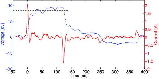
The high voltage pulse is produced by a Blumlein pulse forming network, creating $15\,$ – $35\,$ kV pulses with $130\,$ ns duration and $10\,$ ns rise and fall time. All measurements in this article have been done with positive 25 kV pulses, creating positive streamers emerging from the point electrode. A typical 25 kV voltage pulse and the corresponding current under vacuum conditions are shown in figure 1. The voltage is measured with a Northstar PVM-4 1:1000 voltage probe with a bandwidth of $110\,$ MHz. The current is determined from the voltage across a $50\,\Omega$ shunt resistor between the cathode plane and the grounded vessel. Because the current in figure 1 is measured under vacuum conditions, it is purely capacitive: $C\cdot dV/dt$ . The measurements indicate that the vessel capacitance is $C\approx 1\,$ pF.

Refer to caption — Figure 1: Averaged waveforms of thirty 25 kV Blumlein pulses under vacuum condition (i.e. without discharge). The voltage is shown as the dashed (blue) line. The continuous (red) line shows the current waveform, dominated by the displacement current C dV/dt. The horizontal dashed (black) line indicates the average voltage of the pulse as we report it.

The streamer discharges are imaged with a Stanford Computer Optics 4QuickE iCCD-camera and a Nikkor-UV $105\,$ mm $f/4.5$ UV-lens. This camera is capable of nanosecond delay and shutter control, allowing for precise image timing. More details on the setup can be found in [8].

3 Results

3.1 The variations of the voltage pulse

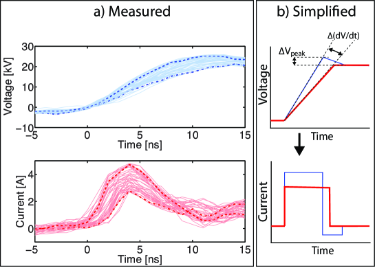
The voltage waveforms measured in our setup vary slightly from pulse to pulse in the rising and falling edges of the voltage pulses. These variations are related to the pulse forming network and we can (currently) not control it. The upper panel in figure 2a shows a series of measured voltage waveforms as a function of time during the time interval from $t=-5\,$ ns up to $t=15\,$ ns around the rising edge. The time axis is defined as in figure 1, with the voltage pulse starting to rise at $t=0\,$ ns. The lower panel in figure 2a shows the corresponding current waveforms. The waveforms shown here are measured under discharge conditions but are essentially identical to waveforms under vacuum conditions because the corona current is still negligible at the start of the voltage pulse.

The variation in the voltage wave form can be described in a simplified manner in terms of voltage slope and peak voltage. Figure 2b illustrates this simplified sketch for the voltage as well as for the corresponding capacitive current. Though the transitions in the actually measured waveforms are, of course, much smoother, the simplified schematic is useful to describe the variation.

For faster rising voltage pulses (with larger voltage slope $\textrm{d}V/\textrm{d}t$ ), the peak voltage $V_{\textrm{peak}}$ is larger as well, as it shows a short voltage overshoot. Taking $\textrm{d}V/\textrm{d}t$ between $t=2\,$ ns and $t=10\,$ ns as a measure, we find that the average slope varies between $1.9\,$ kV/ns and $2.7\,$ kV/ns in the measured waveforms. The maximal difference of the peak voltage $\Delta V_{\textrm{peak}}$ at $t=12\,$ ns is $6\,$ kV.

As far as we have been able to test, the voltage slope varies in a completely random manner. It is neither alternating, nor remaining for a while in one state and then jumping to another state. Our hypothesis for the physical mechanism behind the voltage rise variation is based on the breakdown of our multiple spark-gap. As a part of the Blumlein pulse forming network, the multiple spark-gap consists of seven electrodes that distribute the voltage over six gaps. After the trigger pulse the gaps break down one by one, leaving the full voltage distributed over less many gaps after every gap breakdown. At the final breakdown, the last gap releases the full DC-voltage.

We think that the order of breakdown of the individual gaps may cause the voltage rise variation. The trigger voltage is put across the first and second electrode, thereby changing not only the voltage over the first gap voltage, but also over the second gap. As a consequence, it is not a consecutive breakdown of adjacent gaps that evolves in the multiple spark-gap, but an interplay between gap voltage, gap distance and stochastic variations that lead to variable breakdown sequences and delays. For the multiple spark-gap as a whole, this means that the total breakdown delay may vary, resulting in slightly different voltage rise rates.

3.2 Discharge observations

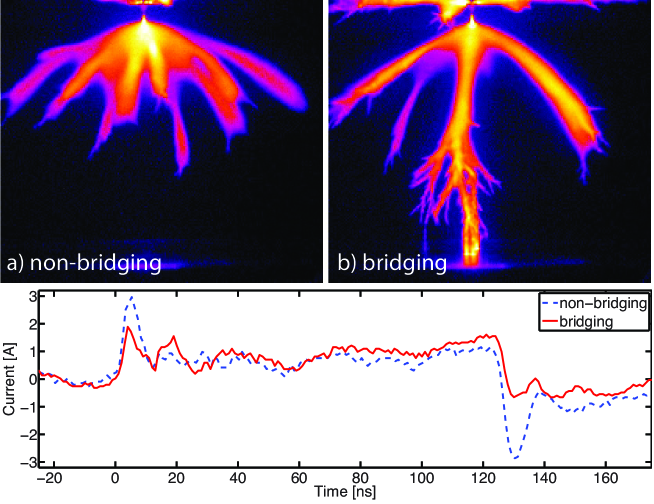
We have observed a structural variation of the discharge behaviour that is related to, and most likely caused by, the voltage pulse variation. Panels a and b in figure 3 show two discharges, and the lower panel shows the corresponding current waveforms. These discharges occurred in the same pulse sequence with fixed parameters: 100 mbar (nitrogen 6.0), 25 kV Blumlein pulses at 5 Hz repetition rate. Note that it has been shown previously [18] that at this repetition rate the influence of leftover background ionization from the previous discharge pulse is significant, creating thick and smooth channels rather than thin and feather-like branches like at low repetition rates. Other interesting aspects of the discharge morphology will be discussed later in section 5.

The discharge in figure 3a does not reach the cathode, while the discharge in figure 3b clearly does. In the discharge sequence of this measurement, the ratio of bridging to non-bridging discharges was about 50/50. Though the difference in the size of the two discharges is large, one must realise that during the latest stage of evolution, the high electric field between the approaching streamer and the cathode plane in the bottom part of the gap as well as possibly secondary emission from the cathode cause a significant acceleration of the channel propagation.

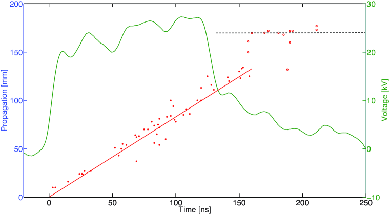
Figure 4 shows the length of the longest streamer channel as a function of time. The longest streamer channel of a discharge has been taken as a measure for the propagation, because it gives a lower boundary for the maximum velocity. Due to the 2D-projection of the discharge on the camera CCD, streamer channels with a component perpendicular to the image plane will appear shorter on the image. Therefore the longest streamer is the best measure for the actual streamer length. Note that all data points represent different discharges, because the camera cannot capture multiple images within one discharge. As a reference, a voltage pulse is also plotted in the figure. The start of the streamer propagation has been aligned with the rise of the voltage pulse.

The figure demonstrates that up to $t=150$ ns the streamers propagate with nearly constant velocity. The linear fit indicated by the solid red line corresponds to a velocity of $(8.3\pm 0.5)\cdot 10^{5}\,$ m/s. After $t=150$ ns, or at a distance of ~40 mm from the cathode plane, the streamers seem to ‘jump’ to the cathode plane whose position is marked with a dashed black line. Streamer lengths near this line represent discharges that have bridged the gap. The final streamer acceleration over the last 40 mm even after the main voltage pulse is probably caused by secondary electron emission from the cathode plane, combined with the field enhancement due to the streamer head charge approaching the planar electrode. In this discharge series, only one discharge has not bridged the gap after $t=150$ ns (data point at $t=185$ ns and $x=130$ mm). As stated before, the bridging to non-bridging ratio of the discharge series discussed in the rest of this article is about 50/50. The fast jump towards the cathode plane over the last 40 mm indicates that the difference in terms of propagation between the two discharges in figure 3 is quite small. Whether a discharges does or does not bridge, could thus in principle be caused by stochastic variations.

However, distinguishing between bridging and non-bridging discharges and analysing the corresponding current waveforms brings up structural differences related to the voltage rise variation. In figure 3, these current waveforms are shown below the discharge images. At the end of the voltage pulse, around $t=125$ ns, there is a significant difference in the current between the bridging and non-bridging discharges. While the non-bridging has a strong negative peak of about $-3\,$ A that corresponds to the displacement current $C\cdot dV/dt$ , the current of the bridging discharge decays only to just below zero. This can be attributed to the higher corona current associated with the bridging of the gap. Because the conductive connection with the cathode plane is formed just before the pulse voltage decreases, a significantly higher corona current flows as opposed to the non-bridging discharge. The negative capacitive current due to the voltage drop, which is clearly visible for the non-bridging discharge, is neutralised by the corona current.

The current waveforms in figure 3 also show a significant difference at the early stage, in the height of the first peak at $t\approx 6\,$ ns. As explained in the previous subsection, this peak corresponds to the capacitive current of the voltage pulse rise. In a measurement series of about thirty discharges, we have observed that structurally the bridging discharge has a lower first current peak. This makes it plausible that the bridging behaviour is linked to the voltage pulse variation.

3.3 Discharge behaviour related to the voltage pulse

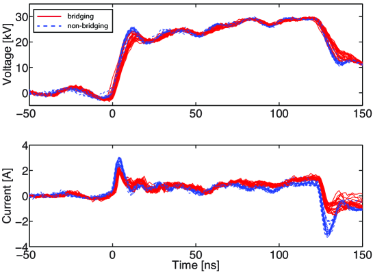
Figure 5 shows the individual voltage and current waveforms of the full discharge sequence. The solid red lines mark all discharges that clearly do not have the strongly negative current peak at the end of the voltage pulse. As discussed in the previous section, this means that these discharges have bridged the gap. The dashed blue lines, on the other hand, indicate the non-bridging discharges.

Just after the start of the discharge pulse, the first current peak of the bridging discharges is clearly lower than for the non-bridging ones. The average peak height is $2.0\pm 0.2\,$ A for the bridging discharges versus $2.8\pm 0.3\,$ A for the non-bridging discharges, which amounts to a significant difference of about a $3\sigma$ . The upper panel in figure 5 shows that the lower initial current peak of the bridging discharge indeed corresponds to a lower voltage rise time of the voltage switch, as argued earlier based on the capacitive nature of this initial current.

4 Physical interpretation

4.1 Formation and size of the inception cloud

How can it be explained that a faster rising and overall higher voltage creates discharges that propagate less far within the same time? Figure 3 shows another difference between bridging and non-bridging discharges: the size of the inception cloud. As shown previously in [19, 8, 18, 20, 21], next to a needle electrode, first an inception cloud grows. This cloud forms an ionization front that propagates outward and is visible as a shell. The shell eventually destabilizes into streamers. Analysing the discharge series, it seems that a faster voltage rise causes a larger inception cloud and correspondingly a later emergence of streamer channels.

The maximal radius $R_{max}$ of the inception cloud as a function of breakdown field $E_{\textrm{br}}$ and applied voltage V can be estimated as $R_{max}=V/E_{\textrm{br}}$ . This estimate is based on the assumption that the inception cloud is spherical and perfectly conducting; then if the cloud is on an electric potential V, and if the electric field on the surface is precisely the breakdown field, the radius is given by the equation above. We remark that the volume of the inception cloud is actually larger than the critical volume (where the electric field exceeds the breakdown field) in the absence of the discharge.

The breakdown field $E_{\textrm{br}}$ in 100 mbar nitrogen is approximately $2\,$ kV/cm. The maximal radius of the inception cloud is therefore 125 mm for a voltage of 25 kV; this is comparable to the size of the gap. However, even in air with its stabilizing effect of photo-ionization, the maximal radius is typically not reached in positive discharges (though a counter example is shown in figure 8d below) while for negative discharges an example can be found in [20] where the discharge cloud reaches approximately the maximal radius. The important fact is, however, that a faster voltage rise creates a more ionized and more stable inception cloud that breaks up later into individual streamer channels.

4.2 The sizes of the whole discharge and of the inception cloud

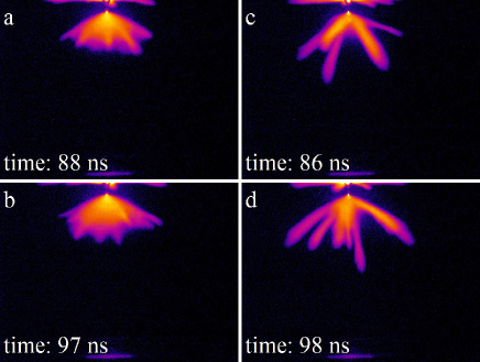
Now the evolution of the whole discharge will be related to the size of the inception cloud. We took time-resolved images of the discharge propagation. Figure 6 shows two sets of images, the upper ones with an exposure time of about 87 ns, the lower ones with about 97 ns. In both cases, the discharges on the left have much larger inception clouds and a smaller overall extension, while on the right the inception clouds are small and the emerged streamers have propagated much further out. We conclude that the inception cloud propagates slower than the individual channels. The explanation lies in the fact that at the same distance from the electrode, the electric field at the tip of a pointed streamer channel is enhanced to much higher values than at the rather flat ionization front around the inception cloud. The higher local field leads to a higher velocity.

Note that figures 6a and b show, that the inception cloud destabilises about $70-90\,$ ns after the start of the voltage pulse. As the rise time of the voltage pulse is only about $10\,$ ns, the actual differences in the inception cloud size are still visible much later, long after the voltage rise. We hypothesize that the more strongly driven early nucleation process of the discharge near the electrode needle during the first 10 ns still influences the stability of the cloud after 60 - 80 ns. The underlying reason could be the higher conductivity of the plasma directly at the electrode which is created at the early stages; a high conductivity there allows a continuous flow of electric current from the electrode into the plasma region. Simulations investigating this hypothesis are currently under development. Note that once the plasma front becomes unstable and starts to branch, the process cannot be reversed. It may continue in that form or branch even further, but it will never return to the homogeneous plasma front it originated from.

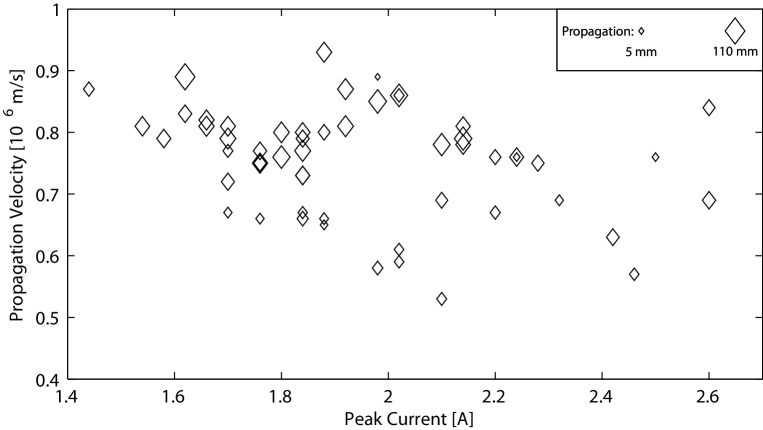
It appears that the inception cloud propagates slower than the streamers at the same distance from the electrode. This behaviour is further investigated in figure 7. It shows the average propagation velocity of the discharge during the exposure time as a function of the peak current (which is proportional to the voltage rise rate). The propagation distance is indicated by the size of the markers. Small diamonds represent measurements early in the discharge formation, whereas large diamonds correspond to almost fully developed discharges (discharges up to $110\,$ mm length have been measured). The larger diamonds show that the final average velocity is about $8\cdot 10^{5}\,$ m/s. For higher peak currents, there are relatively many data points for low velocities. These are mostly small diamonds, showing that the discharge is still small. The figure shows that indeed the discharge propagates more slowly when the peak current is higher (and thus the voltage rise faster).

Another aspect that supports our observation can be found in figure 4. Between 60 ns and 100 ns, a couple of data points significantly deviate from the trend through a shorter propagation length. From the corresponding images we have found that these are discharges with a larger inception cloud, from which no channels have emerged yet - similar to those on the left in figure 6.

We conclude that higher voltage rise times create inception clouds that grow to a larger size before they destabilize into streamers, and that the inception cloud grows more slowly than a streamer at the same distance from the electrode. This is very reasonable, since the electric field at the edge of an inception cloud is lower than at a streamer tip at the same distance from the electrode.

4.3 The inception cloud in air

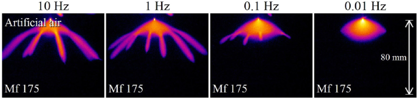
The size of the inception cloud and of the overall discharge behaves similarly in air; as can be found in an investigation of the effects of background ionization on streamer discharges in air and in nitrogen [18]. Figure 3 in that paper compares the observed effects in air and nitrogen. The paper as well as our figure 8 that is reproduced from [18] show that discharges in air behave similarly as discharges in nitrogen 6.0: a larger inception cloud coincides with a smaller overall discharge size within the same evolution time. Based also on our theoretical understanding, we hypothesize that this behaviour is valid in other gases as well. We also expect the influence of the voltage rise rate to be a general discharge effect, independently of the gas composition.

We conclude with two remarks on the discharge in air shown in figure 8. 1. The inception clouds in air are always much larger than in nitrogen under similar conditions; this is due to the stabilizing effect of the non-local photo-ionization reaction. The inception cloud in the rightmost panel of the figure is almost 30 mm which is close to the maximal radius predicted to be about 40 mm. This is the case even though the discharge is positive, and therefore more unstable. 2. Discharges at higher repetition rates develop a smaller inception cloud and their streamer channels propagate further. The higher repetition rate creates a higher background density [18]. But why a higher background ionization destabilizes the cloud earlier, is not understood yet, as the traces of the previous discharges are smoothed out by diffusion by the time of the next voltage pulse. In nitrogen we see and understand the opposite effect.

5 Discharge morphology: local branching reduction

The discharges in figure 3 have more interesting features besides their relation to the voltage rise rate. It was already noted by Nijdam et al.[18] that at the present repetition rate of 5 Hz the remaining ionization of the previous discharge pulse has a significant effect on the next discharge in nitrogen 6.0. Nijdam et al. conclude that the abundance of seed electrons reduces the stochastic fluctuations of electron density ahead of the ionization front of streamers or of the inception cloud, and that they therefore destabilize and branch later than in virgin gas [22]. In the lower part of the discharge in figure 3b, however, the channels are thinner and branch more, similarly to discharge in a lower background ionization. This observation is consistent with calculations in [18] that indicate that ionization created in the upper part of the discharge will not reach the lower discharge region in the time between consecutive voltage pulses.

An elegant experiment by Takahashi [23] shows that streamer branching can be controlled locally by irradiating an (argon) discharge at atmospheric pressure with a laser. From their results they deduce that ionization levels higher than $5\times 10^{5}\,$ cm^-3 influence streamer branching.

Both experiments show that the remaining ionization of a previous discharge pulse has local effects on the subsequent discharge for the discharge volume and gas considered here.

Similarly to the experiments performed by Takahashi, we have performed measurements to verify that a higher background ionization density reduces branching locally. The hypothesis is that at the next discharge pulse, there is non-uniform ionization remaining from the previous discharge(s). The pre-ionized volume and ionization density in pure nitrogen is determined by diffusion and recombination. When diffusion is fast, the remaining ionization is expected to be non-local and uniform, whereas for slow diffusion we expect to see clear local effects of the remaining ionization on the branching behaviour of the subsequent discharge.

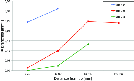
Figure 9a shows the branching rate of three subsequent discharges after a long pause. The pause is much longer than one minute, and experiments and calculations agree on the fact that after more than one minute, there are no visible effects of previous discharges left. The graph shows the number of (manually counted) branches per millimetre of streamer channel length as a function of the distance to the tip (grouped) for the first, second and third discharge after the pause. The number of branches is evaluated by selecting a certain part of a streamer channel and counting its branches. It can be seen clearly that the branching rate decreases for subsequent discharges, but only in the volume of the preceding discharge.

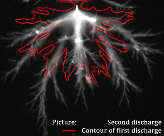
The effect of the first discharge on the second one at 5 Hz repetition frequency is visualised in a different manner in figure 9b; here a picture of the second discharge is overlayed with a contour sketch of the first discharge. Of course this is only a 2D-projection, but it is clearly visible that branching is suppressed within the contour of the first discharge. Note that the channels of subsequent discharges do not follow the exact same path (as was also shown in [18]). Branching is suppressed in the second discharge within roughly the whole (semi-)spherical volume of the first discharge, with a smooth transition outwards. This behaviour is consistent with the estimated diffusion length of pre-ionization within the available time, also calculated in [18], where the diffusion length after 0.2 s in 200 mbar pure nitrogen was found to be about 7 mm (see figure 6 of that work). At 100 mbar this length will double so that the pre-ionization is spread out over the whole (semi-)spherical volume covered by the discharge.

To the best of our knowledge, this is the first experiment that shows the build-up of pre-ionization in the discharge volume in repetitive discharges and its local influence on the morphology of subsequent discharges.

Another peculiarity that can be observed in figures 3b and 9b: is the structure about two-thirds of the distance between tip and plate. It shows a very sudden transition from thick, non-branching channels to many much thinner and feather-like branches that propagate into quite different directions. We name this structure a ‘knotwilg’, after the Dutch name for a pollard willow tree with a thick stem and many thin branches (that are harvested regularly). We will address possible explanations for this structure in future work.

6 Conclusions

We have investigated positive streamer discharges in high purity nitrogen at 100 mbar, generated by voltage pulses of 130 ns duration at 5 Hz repetition. We have shown that a slight variation in the voltage rise rate between different pulses has an important impact on the dynamics and morphology of the discharges. The voltage rise is characterised by the slope, which varies from $1.9\,$ kV/ns to $2.7\,$ kV/ns, and by the peak voltage, ranging from $22\,$ kV to $28\,$ kV.

Pulses with a faster rise rate create more compact discharges within the duration of the pulse and thus have a lower average propagation velocity. This difference appears to arise during the first phase of streamer formation, because the more compact discharges have a larger inception cloud. Time resolved measurements indicate that the inception cloud extends indeed slower than streamer channels. This can be immediately understood as the electric field enhancement at the edge of a (round) inception cloud is lower than at a (pointed) streamer tip.

The maximal size of the inception cloud depends on the voltage. Approximating the cloud as an ideally conductive sphere, its maximal radius is $R_{max}=V/E_{\textrm{br}}$ , where $V$ is the applied potential and $E_{\textrm{br}}$ the breakdown field of the gas. Therefore both our understanding and our measurements suggest that a faster voltage rise creates a larger and more stable inception cloud, thereby delaying the destabilisation into streamer channels. Therefore after the 130 ns voltage pulse, the discharge reaches out less far than with a lower voltage rise rate. We believe that this relation between voltage rise rate, size of inception cloud and spatial extension of the complete discharges holds in other gases as well.

We also investigate the consequences of pulse repetition for the discharge morphology. Remaining pre-ionization of previous discharge pulses creates thicker streamers and a lower branching rate as shown previously in [18]. We find that the effects of pre-ionization are constrained to the volume of the previous discharge, in agreement with estimates of the diffusion length between pulses. Like in the experiments of Takahashi [23], the pre-ionization has localised effects on the discharge.

References

[1] J. S. Clements, A. Mizuno, W. C. Finney, and R. H. Davis. Combined removal of SO₂, NO_x, and fly ash from simulated flue gas using pulsed streamer corona. IEEE T. Ind. Appl., 25(1):62 –69, jan. 1989.
[2] L. Grabowski, E. van Veldhuizen, A. Pemen, and W. Rutgers. Corona above water reactor for systematic study of aqueous phenol degradation. Plasma Chem. Plasma Process., 26:3–17, 2006. 10.1007/s11090-005-8721-8.
[3] E. M. van Veldhuizen. Electrical Discharges for Environmental Purposes: Fundamentals and Applications. Nova Science Publishers, New York, 2000.
[4] G. J. J. Winands, Keping Yan, A. J. M. Pemen, S. A. Nair, Zhen Liu, and E. J. M. van Heesch. An industrial streamer corona plasma system for gas cleaning. IEEE T. Plasma Sci., 34(5, Part 4):2426–2433, OCT 2006.
[5] U. Kogelschatz. Atmospheric-pressure plasma technology. Plasma Phys. Contr. F., 46(12B):B63, 2004.
[6] Eric Moreau. Airflow control by non-thermal plasma actuators. J. Phys. D: Appl. Phys., 40(3):605, 2007.
[7] A.Y. Starikovskii, N.B. Anikin, I.N. Kosarev, E.I. Mintoussov, M.M. Nudnova, A.E. Rakitin, D.V. Roupassov, S.M. Starikovskaia, and V.P. Zhukov. Nanosecond-pulsed discharges for plasma-assisted combustion and aerodynamics. J. Propul. Power, 24(6):1182, 2008.
[8] S. Nijdam, F. M. J. H. van de Wetering, R. Blanc, E. M. van Veldhuizen, and U. Ebert. Probing photo-ionization: Experiments on positive streamers in pure gases and mixtures. J. Phys. D: Appl. Phys., 43:145204, 2010.
[9] Sander Nijdam. Experimental Investigations on the Physics of Streamers. PhD thesis, Eindhoven University of Technology, 2011. http://alexandria.tue.nl/extra2/693618.pdf.
[10] D. Dubrovin, S. Nijdam, E. M. van Veldhuizen, U. Ebert, Y. Yair, and C. Price. Sprite discharges on Venus and Jupiter-like planets: a laboratory investigation. J. Geophys. Res. - Space Physics, 115:A00E34, 2010.
[11] T. M. P. Briels, J. Kos, E. M. van Veldhuizen, and U. Ebert. Circuit dependence of the diameter of pulsed positive streamers in air. J. Phys. D: Appl. Phys., 39:5201, 2006.
[12] T. M. P. Briels, J. Kos, G. J. J. Winands, E. M. van Veldhuizen, and U. Ebert. Positive and negative streamers in ambient air: measuring diameter, velocity and dissipated energy. J. Phys. D: Appl. Phys., 41:234004, 2008.
[13] G. J. J Winands, Z. Liu, A. J. M. Pemen, E. J. M. van Heesch, K. Yan, and E. M. van Veldhuizen. Temporal development and chemical efficiency of positive streamers in a large scale wire-plate reactor as a function of voltage waveform parameters. J. Phys. D: Appl. Phys., 39:3010, 2006.
[14] E. J. M. van Heesch, G. J. J Winands, and A. J. M. Pemen. Evaluation of pulsed streamer corona experiments to determine the O* radical yield. J. Phys. D: Appl. Phys., 41(23):234015, 2008.
[15] I. Yagi, S. Okada, T. Matsumoto, Douyan Wang, T. Namihira, and K. Takaki. Streamer propagation of nanosecond pulse discharge with various rise times. Plasma Science, IEEE Transactions on, 39(11):2232 –2233, nov. 2011.
[16] G. J. J Winands, Z. Liu, A. J. M. Pemen, E. J. M. van Heesch, and K. Yan. Analysis of streamer properties in air as function of pulse and reactor parameters by iccd photography. J. Phys. D: Appl. Phys., 41:234001, 2008.
[17] Q.G. Zhang, F.B. Tao, Z. Li, W.D. Ding, and A.C. Qiu. Effect of pulse rise time on the glow discharge in nonuniform electric field. Plasma Science, IEEE Transactions on, 36(4):1008 –1009, aug. 2008.
[18] S. Nijdam, G. Wormeester, E. M. van Veldhuizen, and U. Ebert. Probing background ionization: positive streamers with varying pulse repetition rate and with a radioactive admixture. J. Phys. D: Appl. Phys., 44(45):455201, 2011.
[19] T. M. P. Briels, E. M. van Veldhuizen, and U. Ebert. Time resolved measurements of streamer inception in air. IEEE T. Plasma Sci., 36(4):908–909, 2008.
[20] S. Nijdam, K. Miermans, E.M. van Veldhuizen, and U. Ebert. A peculiar streamer morphology created by a complex voltage pulse. IEEE T. Plasma. Sci., 2011. Submitted.
[21] U. Ebert, F. Brau, G. Derks, W. Hundsdorfer, C.-Y. Kao, C. Li, A. Luque, B. Meulenbroek, S. Nijdam, V. Ratushnaya, L. Schäfer, and S. Tanveer. Multiple scales in streamer discharges, with an emphasis on moving boundary approximations. NonLinearity, 24:C1, 2011.
[22] A. Luque and U. Ebert. Electron density fluctuations accelerate the branching of streamer discharges in air. Phys. Rev. E, 84:046411, 2011.
[23] E Takahashi, S Kato, A Sasaki, Y Kishimoto, and H Furutani. Controlling branching in streamer discharge by laser background ionization. J. Phys. D: Appl. Phys., 44(7):075204, 2011.