Coordination in Network Security Games:
a Monotone Comparative Statics Approach

Abstract

Malicious softwares or malwares for short have become a major security threat. While originating in criminal behavior, their impact are also influenced by the decisions of legitimate end users. Getting agents in the Internet, and in networks in general, to invest in and deploy security features and protocols is a challenge, in particular because of economic reasons arising from the presence of network externalities.

In this paper, we focus on the question of incentive alignment for agents of a large network towards a better security. We start with an economic model for a single agent, that determines the optimal amount to invest in protection. The model takes into account the vulnerability of the agent to a security breach and the potential loss if a security breach occurs. We derive conditions on the quality of the protection to ensure that the optimal amount spent on security is an increasing function of the agent’s vulnerability and potential loss. We also show that for a large class of risks, only a small fraction of the expected loss should be invested.

Building on these results, we study a network of interconnected agents subject to epidemic risks. We derive conditions to ensure that the incentives of all agents are aligned towards a better security. When agents are strategic, we show that security investments are always socially inefficient due to the network externalities. Moreover alignment of incentives typically implies a coordination problem, leading to an equilibrium with a very high price of anarchy.

I Introduction

Negligent users who do not protect their computer by regularly updating their antivirus software and operating system are clearly putting their own computers at risk. But such users, by connecting to the network a computer which may become a host from which viruses can spread, also put (a potentially large number of) computers on the network at risk [2, 3]. This describes a common situation in the Internet and in enterprise networks, in which users and computers on the network face epidemic risks. Epidemic risks are risks which depend on the behavior of other entities in the network, such as whether or not those entities invest in security solutions to minimize their likelihood of being infected. [4] is a recent OECD survey of the misaligned incentives as perceived by multiple stake-holders. Our goal in this paper is to study conditions for alignment of incentives for agents of a large network subject to epidemic risks and its implications for the equilibria.

Our work allows a better understanding of economic network effects: there is a total effect if one agent’s adoption of a protection benefits other adopters and there is a marginal effect if it increases others’ incentives to adopt it (we refer to Section 3 of [5] for a comprehensive survey about network effects). In information security economics, the presence of the total effect has been the focus of various recent works starting with Varian’s work [6]. When an agent protects itself, it benefits not only to those who are protected but to the whole network. Indeed there is also an incentive to free-ride the total effect. Those who invest in self-protection incur some cost and in return receive some individual benefit through the reduced individual expected loss. But part of the benefit is public: the reduced indirect risk in the economy from which everybody else benefits. As a result, the agents invest too little in self-protection relative to the socially efficient level. The efficiency loss (referred to as the price of anarchy) has been quantified in various game-theoretic models [7, 8, 9, 10, 11, 12].

In this paper, we focus on the marginal effect and its relation to the coordination problem (see Section 3.4 in [5]). To understand the mechanism of incentives regarding security in a large network, we need to analyze how an increase in the total population adopting security will impact one agent’s incentive to adopt it. To do so, we use a monotone comparative statics approach and start with an economic model for a single agent that determines the optimal amount to invest in protection. We follow the approach proposed by Gordon and Loeb in [13]. They found that the optimal expenditures for protection of an agent do not always increase with increases in the vulnerability of the agent. Crucial to their analysis is the security breach probability function which relates the security investment and the vulnerability of the agent with the probability of a security breach after protection. This function can be seen as a proxy for the quality of the security protection. Our first main result (Theorem 1) gives sufficient conditions on this function to ensure that the optimal expenditures for protection always increase with increases in the vulnerability of the agent (this sensitivity analysis is called monotone comparative statics in economics). From an economic perspective, these conditions will ensure that all agents with sufficiently large vulnerability value the protection enough to invest in it. We also extend a result of [13] and show (Theorem 2) that if the security breach probability function is log-convex in the investment, then a risk-neutral agent never invests more than 37% of the expected loss.

Building on these results, we study a network of interconnected agents subject to epidemic risks. We model the effect of the network through a parameter $\gamma$ describing the information available to the agent and capturing the security state of the network. We show that our general framework extends previous work [8, 14] and allows to consider a security breach probability function depending on the parameter $\gamma$ and possibly other private informations on the vulnerability of the asset. Our third main result (Theorem 3) gives sufficient conditions on this function to ensure that the optimal protection investment always increases with an increase in the security state of the network.

This property will be crucial in our last analysis: we use our model of interconnected agent in a game theoretic setting where agents anticipate the effect of their actions on the security level of the network. We diverge form most of the literature on security games (some exceptions are [15, 8, 16]) and relax the complete information assumption, i.e. each player’s security breach probability is not common knowledge but instead a private information. In our model only global statistics are publicly available and agents do not disclose any information concerning their own security strategy.

We show how the monotonicities (or the lack of monotonicities) impact the equilibrium of the security game. In particular, alignment of incentives typically implies a coordination problem, leading to an equilibrium with a very high price of anarchy. Moreover, we distinguish two parts in the network externalities that we call public and private. Both types of externalities are positive since any additional agent investing in security will increase the security level of the whole network. However, the effect of this additional agent will be different for an agent who did not invest in security from an agent who already did invest in security. The public externalities correspond to the network effect on insecure agents while the private externalities correspond to the network effect on secure agents (also called total effect in the economics literature [5]).

As a result of this separation of externalities, some surprising phenomena can occur: also both externalities are positive, there are situations where the incentive to invest in protection decreases as the fraction of the population investing in protection increases. This is an example where the total effect holds but the marginal effect fails (which is essentially a case where Segal’s increasing externalities [17] or Topkis’supermodularity [18] fails). We also show that in the security game, security investments are always inefficient due to the network externalities. This raises the question whether economic tools like insurance [19, 20, 21] could be used to lower the social inefficiency of the game?

The rest of the paper is organized as follows. In Section II, the optimal security investment for a single agent is analyzed. In Section III, we extend it to an interconnected agent and show it connects with the epidemic risk model. Finally in Section IV, we consider the case where agents are strategic. We introduce the notion of fulfilled expectations equilibrium and show our main game theoretic results.

II Optimal security investment for a single agent

In this section, we present a simple one-period model of an agent contemplating the provision of additional security to protect a given information set introduced by Gordon and Loeb in [13]. In one-period economic models, all decisions and outcomes occur in a simultaneous instant. Thus dynamic aspects are not considered.

II-A Economic model of Gordon and Loeb

The model is characterized by two parameters $\ell$ and $v$ (also Gordon and Loeb used a bit more involved notation). The parameter $\ell$ represents the monetary loss caused by a security breach. The parameter $\ell\in\mathbb{R}_{+}$ is a positive real number. The parameter $v$ represents the probability that without additional security, a threat results in the information set being breached and the loss $\ell$ occurs. The parameter $v$ is called the vulnerability of the asset. Being a probability, it belongs to the interval $[0,1]$.

An agent can invest a certain amount $x$ to reduce the probability of loss to $p(x,v)$. We make the assumptions $p(0,v)=v$ and since $p(x,v)$ is a probability we assume that for all $x>0$ and $v\in[0,1]$ we have $0\leq p(x,v)\leq v$. The function $p(x,v)$ is called the security breach probability.

The expected loss for an amount $x$ spent on security is given by $\ell p(x,v)$. Hence if the agent is risk neutral, the optimal security investment should be the value $x^{*}$ minimizing

$$\min\left\{\ell p(x,v)+x:x\geq 0\right\}.$$ (1)

We define the set of optimal security investment by $\varphi(v,\ell)=\arg\min\left\{\ell p(x,v)+x:x\geq 0\right\}$. Clearly in general the function $\varphi$ is set-valued and we will deal with this fact in the sequel. For now on, assume that the function $\varphi$ is real-valued, i.e. sets reduce to singleton. As noticed in [13], it turns out that the function $\varphi(v,\ell)$ does not need to be non-decreasing in $(v,\ell)$ for general functions $p(x,v)$. An example given in [13] is $p_{GL}(x,v)=v^{\alpha x+1}$, where the parameter $\alpha>0$ is a measure of the productivity of information security. This class of security breach probability functions has the property that the cost of protecting highly vulnerable information sets becomes extremely expensive as the vulnerability of the information set becomes very close to one. This is not the only class of security breach functions with this property. Their simplicity allows to gain further insights into the relationship between vulnerability and optimal security investment.

Indeed, an interior minimum $x^{*}>0$ is characterized by the first-order condition:

$$\ell\frac{\partial p}{\partial x}(x^{*},v)=-1.$$ (2)

In the particular case where $p_{GL}(x,v)=v^{\alpha x+1}$, we obtain $\frac{\partial p_{GL}}{\partial x}(x,v)=(\alpha\log v)v^{\alpha x+1}$. So that solving Equation (2), we get $\varphi_{GL}(v,\ell)=\frac{-\log\left(-\ell\alpha\log v\right)}{\alpha\log v}-\frac{1}{\alpha}$.

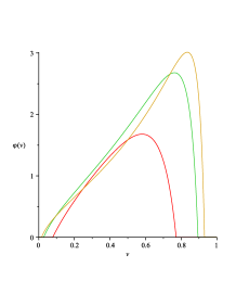
Figure 1: Function $\varphi_{GL}(v,\ell)$ as a function of the vulnerability $v$ and with parameters: $\ell=10$ and $\alpha=0.5,1,1.5$ (red, green, brown)

Figure 1 shows the optimal security investment for various values of $\alpha$ and $\ell$ as a function of the vulnerability $v$. In particular, we see that the optimal investment is zero for low values of the vulnerability and also for high values of the vulnerability. In other words, in this case, the marginal benefit from investment in security for low vulnerability information sets does not justify the investment since the security of the information set is already good. However if the information set is extremely vulnerable, the cost of security is too high to be ’profitable’, in the sense that there is no benefit in protecting it.

II-B Sufficient conditions for monotone investment

In this section, we derive sufficient conditions on the probability loss in order to avoid the non-monotonicity in the vulnerability of the information set. In such a case, the information security decision is simple since there is an augmenting return of investment with vulnerability: the security manager needs to adjust the security investment to the vulnerability. Also the security provider should set the price of its solution so as to remain in a region where such monotonicity is valid.

First we need to define the monotonicity of a set-valued function. We say that the set-valued function $f:\mathbb{R}^{n}\to 2^{\mathbb{R}}$ is non-decreasing if for any $x^{L},x^{H}\in\mathbb{R}^{n}$ with $x^{L}\leq x^{H}$ (for the product order), we have for any $y^{L}\in f(x^{L})$ and any $y^{H}\in f(x^{H})$: $y^{L}\leq y^{H}$.

We start with a particular case (its proof will follow from our more general result and is given at the end of this section):

Proposition 1.

Assume that the function $p(x,v)$ is twice continuously differentiable on $\mathbb{R}_{+}\times[0,1]$. If

$$\frac{\partial p}{\partial x}(x,v)\leq 0, \frac{\partial^{2}p}{\partial x\partial v}(x,v)\leq 0$$ and, (3)

then the function $(v,\ell)\mapsto\varphi(v,\ell)$ is non-decreasing in $(v,\ell)$.

Remark 1.

The first condition requires that the function $p(x,v)$ is non-increasing in $x$, i.e. the probability of a security break is lowered when more investment in security is done. In the particular case of $p_{GL}$ described above, we have $\frac{\partial^{2}p_{GL}}{\partial x\partial v}(x,v)=\alpha v^{\alpha x}\left(1+\alpha(\alpha x+1)\log v\right)$. In particular $\frac{\partial^{2}p_{GL}}{\partial x\partial v}(x,1)=\alpha>0$ and we see that the function $p_{GL}$ does not satisfy the conditions of the proposition which is in agreement with the fact that the associated function $\varphi_{GL}$ is not monotone in $v$.

It turns out that we often need to deal with cases where the choice sets are discrete. In reality, discrete investments in new security technologies are often more natural, resulting in discontinuities. For example the amount $x$ could live in a space $X\subset\mathbb{R}_{+}$ having empty interiors. In these cases, Proposition 1 is useless. In order to extend it, we introduce the notion of general submodular functions (see Topkis [22]). We first define the two operators $\wedge$ and $\vee$ in $\mathbb{R}^{n}$:

$$x\wedge y = \sup\{t\in\mathbb{R}^{n},\>t\leq x;\>t\leq y\}\mbox{and,}$$

$$x\vee y = \inf\{t\in\mathbb{R}^{n},\>t\geq x;\>t\geq y\}.$$

A set $S\subset\mathbb{R}^{n}$ is a lattice if for any $x$ and $y$ in $S$, the elements $x\wedge y$ and $x\vee y$ are also in $S$. A real valued function $f$ on a lattice $S$ is submodular if for all $x$ and $y$ in $S$, $f(x\wedge y)+f(x\vee y)\leq f(x)+f(y)$. $f$ is strictly submodular on $S$ if the inequality is strict for all pairs $x,y$ in $S$ which cannot be compared with respect to $\geq$, i.e such that neither $x\geq y$ nor $y\geq x$ holds.

We are now ready to state our main first result which is an adaptation of Theorem 6.1 in [22]:

Theorem 1.

Let $S=[0,1]\times\mathbb{R}_{+}$. If the function $f:X\times S\to\mathbb{R}$ is strictly submodular in the variables $x$ and $v$ in $X\times[0,1]$ for any fixed $\ell$ and in the variables $x$ and $\ell$ in $X\times\mathbb{R}_{+}$ for any fixed $v$, then $\varphi(v,\ell)=\arg\min\{f(x,v,\ell):\>x\in X\}$ is non-decreasing.

Remark 2.

Note that this Theorem does not require to take $f(x,v,\ell)=\ell p(x,v)+x$. In particular it can also be applied to the case of risk-adverse agents in which case $f$ depends on the (concave) expected utility function of the agent.

Proof.

If $x\leq x^{\prime}$ and $x\neq x^{\prime}$, then $x<x^{\prime}$ is written. By the definition of strict submodularity, we see that we have for $x^{\prime}>x$ and $(v^{\prime},\ell^{\prime})>(v,\ell)$:

$$f(x^{\prime},v^{\prime},\ell^{\prime})+f(x,v,\ell^{\prime}) < f(x^{\prime},v,\ell^{\prime})+f(x,v^{\prime},\ell^{\prime})$$

$$f(x^{\prime},v,\ell^{\prime})+f(x,v,\ell) < f(x^{\prime},v,\ell)+f(x,v,\ell^{\prime}),$$

so that we get

$$f(x^{\prime},v^{\prime},\ell^{\prime})+f(x,v,\ell) < f(x^{\prime},v,\ell)+f(x,v^{\prime},\ell^{\prime}).$$

This shows that $f$ has strictly increasing differences in $(x,v,\ell)$, i.e. $f(x,v,\ell)-f(x,v^{\prime},\ell^{\prime})$ is strictly increasing in $x$ for all $(v^{\prime},\ell^{\prime})>(v,\ell)$.

Consider $(v^{\prime},\ell^{\prime})>(v,\ell)$ and we now show that $y\geq x$ for $y\in\varphi(v^{\prime},\ell^{\prime})$ and $x\in\varphi(v,\ell)$. Suppose that $x>y$, so that $x\vee y>y$. Since $y\in\varphi(v^{\prime},\ell^{\prime})$ and $x\in\varphi(v,\ell)$, we have

$$f(x\vee y,v^{\prime},\ell^{\prime}) \geq f(y,v^{\prime},\ell^{\prime})\mbox{ and, }$$

$$f(x\wedge y,v,\ell) \geq f(x,v,\ell).$$

Using the fact that $f$ has strictly increasing differences, and $x\vee y>y$, we get:

$$f(x\vee y,v^{\prime},\ell^{\prime})-f(y,v^{\prime},\ell^{\prime}) < f(x\vee y,v,\ell)-f(y,v,\ell).$$

By the definition of submodularity, we have:

$$f(x\vee y,v,\ell)-f(y,v,\ell) \leq f(x,v,\ell)-f(x\wedge y,v,\ell)$$

Hence we finally get:

$$0 \leq f(x\vee y,v^{\prime},\ell^{\prime})-f(y,v^{\prime},\ell^{\prime})$$

$$< f(x,v,\ell)-f(x\wedge y,v,\ell)\leq 0,$$

which provides the desired contradiction. ∎

Remark 3.

It follows from the proof, that the sufficient conditions on $f$ to insure that $\varphi$ is non-decreasing, are equivalent to: $f(x,v,\ell)-f(x,v^{\prime},\ell^{\prime})$ is strictly increasing in $x$ for all $(v^{\prime},\ell^{\prime})>(v,\ell)$.

Proof.

of Proposition 1:
It follows from the definition of submodularity, that if $f$ is twice-continuously differentiable, then $\frac{\partial^{2}f}{\partial x\partial v}(x,v,\ell)\leq 0$ implies that $f$ is strictly submodular in the variables $x$ and $v$ in $X\times[0,1]$ for any fixed $\ell$. Taking, $f(x,v,\ell)=\ell p(x,v)+x$, we get $\frac{\partial^{2}f}{\partial x\partial v}(x,v,\ell)=\ell\frac{\partial^{2}p}{\partial x\partial v}(x,v)$, we get one of the condition of Proposition 1. The other condition comes from the symmetric condition on $f$: $\frac{\partial^{2}f}{\partial x\partial\ell}(x,v,\ell)\leq 0$. ∎

II-C A simple model and the $1/e$ rule

Consider now a scenario, where there are $K$ possible protections, where $K$ can be infinite. Each protection $j$ is characterized by a cost denoted $x_{j}>0$ and a function $s_{j}(v)$ from $[0,1]$ to $[0,1]$ with the following interpretation: if the system has a probability of loss $v$ without the protection $j$, applying the protection $j$ will lower this probability by a factor of $s_{j}(v)$ (at a cost $x_{j}$)

If an agent applies two different protections say $i$ and $j$, then we will assume that the resulting probability of loss is $s_{i}(v)s_{j}(v)$. The rational behind this assumption is that the protections are independent in a probabilistic sense. The probability of a successful attack is the product of the probabilities to elude each of the protections.

For a total budget of $x$, the agent will choose the subset $J\in[K]=\{1,2,\dots,K\}$ such that $\sum_{j\in J}x_{j}\leq x$ and which minimizes the final probability of loss $\prod_{j\in J}s_{j}(v)$. Hence we define the function $p:\mathbb{R}_{+}\to\mathbb{R}_{+}$ by, $p(x,v)=\inf\left\{\prod_{j\in J}s_{j}(v)\mbox{ s.t }\sum_{j\in J}x_{j}\leq x\right\}$, so that the optimal security investment problem is still given by (1). The problem of deriving the function $p(x,v)$ is a standard integer linear programming problem which can be rewritten as follows $\log p(x,v)=\inf\left\{\sum_{i\in[K]}e_{i}\log s_{j}(v)|\>e_{i}\in\{0,1\},\sum_{i\in[K]}e_{i}x_{i}\leq x\right\}$.

Our aim here is not to address issues dealing with complexity (this problem is known as the knapsack problem) and we will consider the relaxed problem where $e_{i}\in[0,1]$. In this case, the problem is a linear program which is a convex optimization problem. The important thing for us is that the function $x\mapsto p(x,v)$ is log-convex in $x$. We then have the following generalization of Gordon and Loeb’s Proposition 3:

Theorem 2.

If the function $x\mapsto p(x,v)$ is non-increasing and log-convex in $x$ then the optimal security investment is bounded by $\ell v/e$.

Proof.

We denote $x^{*}$ the optimal investment and $p^{*}=p(x^{*},v)$, so that

$$\ell p^{*}+x^{*}\leq\ell p(x,v)+x.$$ (4)

We denote $f(x)=\log\ell p(x,v)$. Firs assume that $x\mapsto p(x,v)$ is continuously differentiable so that we have

$$f(x) \geq f(x^{*})+f^{\prime}(x^{*})(x-x^{*})$$ (5)

$$= \log\ell p^{*}-\frac{1}{\ell p^{*}}(x-x^{*}),$$

where, in the last equality, we used (2). Hence we have, $f(0)\geq\log\ell p^{*}+\frac{x^{*}}{\ell p^{*}}$, which can be rewritten as

$$\ell v\frac{x^{*}}{\ell p^{*}}\exp\left(-\frac{x^{*}}{\ell p^{*}}\right)\geq x^{*}.$$

The theorem follows in this case from the observation that $z\exp(-z)\leq e^{-1}$ for $z\geq 0$.

If we do not assume that $x\mapsto p(x,v)$ is continuously differentiable, we will show (5) using (4). Namely, suppose there exists $x^{\prime}\geq 0$ such that

$$f(x^{\prime})<\log\ell p^{*}-\frac{1}{\ell p^{*}}(x^{\prime}-x^{*}).$$

Then by convexity, we have for any $\alpha\in[0,1]$,

$$f(\alpha x^{\prime}+(1-\alpha)x^{*}) \leq f(x^{*})+\alpha\left(f(x^{\prime})-f(x^{*})\right)$$

$$< \log\ell p^{*}-\frac{\alpha}{\ell p^{*}}(x^{\prime}-x^{*}).$$

However, by (4), we also have

$$f(\alpha x^{\prime}+(1-\alpha)x^{*}) \geq \log\left(\ell p^{*}-\alpha(x^{\prime}-x^{*})\right)$$

$$= \log\ell p^{*}-\frac{\alpha}{\ell p^{*}}(x^{\prime}-x^{*})+O(\alpha^{2}),$$

and we obtain a contradiction. Hence (5) is still true in this case and we can finish the proof as above so that the statement of the theorem holds. ∎

Theorem 2 shows that for a broad class of information security breach probability function, the optimal security investment is always less than 37% of the expected loss without protection. Note that the function $p_{GL}$ introduced above does not satisfy the conditions of Theorem 1 but is log-convex so that in this case, the optimal security investment is always less than 37% of the expected loss. Indeed, we saw that for high values of the vulnerability, the optimal investment is zero. We end this section with another function $p(x,v)=\frac{v}{(ax+1)^{b}}$ with $a,b>0$, which satisfies both the conditions of Theorems 1 and 2. Hence in this case, the optimal security investment increases with the vulnerability but remains below 37% of the expected loss without protection.

III Optimal security investment for an interconnected agent

We now extend the previous framework in order to model an agent who needs to decide the amount to spend on security if this agent is part of a network. In this section, we give results concerning the incentives of an agent in a network. In the next section, we will consider a security game associated to this model of agent and determine the equilibrium outcomes.

III-A General model for an interconnected agent

In order to capture the effect of the network, we will assume that each agent faces an internal risk and an indirect risk. As explained in the introduction, the indirect risk takes into account the fact that a loss can propagate in the network. The estimation of the internal risk depends only on private information available to the agent. However in order to decide on the amount to invest in security, the agent needs also to evaluate the indirect risk. This evaluation depends crucially on the information on the propagation of the risk in the network available to the decision-maker. We now describe an abstract and general setting for the information of the agent.

We assume that the information concerning the impact of the network on the security of the agent is captured by a parameter $\gamma$ living in a partially ordered set $\Gamma$ (poset, i.e a set on which there is a binary relation that is reflexive, antisymmetric and transitive). Indeed this assumption is not a technical assumption. The interpretation is as follows: $\gamma$ captures the state of the network from the point of view of security and we need to be able to compare secure states from unsecure ones.

Given $\gamma\in\Gamma$, the agent is able to compute the probability of loss for any amount $x\in X$ invested in security which is denoted by $p(x,v,\gamma)$. We still assume that the agent is risk neutral , so that the optimal security investment is given by:

$$\varphi(v,\ell,\gamma)=\arg\min\{\ell p(x,v,\gamma)+x:\>x\in X\}.$$ (6)

Note that in our model we consider that only global statistics about the network are available to all agents. The state of the network $\gamma$ is public. A ’high’ value of $\gamma$ corresponds to a secure environment, typically with a high fraction of the population investing in security while a ’low’ value of $\gamma$ corresponds to an unsecure environment with few people investing in security. For example, in the epidemic risk model described below, decision regarding investment are binary and the public information consists of the parameters of the epidemic risk model (which are supposed to be fixed) and the fraction $\gamma$ of the population investing in security. Then for any $\gamma\in[0,1]$, the agent is able to compute $p(x,v,\gamma)$ as explained below. Note that in our model, the vulnerability $v$ of an agent is an intrinsic parameter of this agent, in particular it does not depend on the behavior of others or $\gamma$.

III-B Epidemic risks model

In order to gain further insight, we consider in this section the case of economic agents subject to epidemic risks. This model was introduced in [8]. We concentrate here on a simplified version presented in [14]. In this section, we focus on the dependence of $p(x,v,\gamma)$ in $x$ and $\gamma$. For ease of notation, we remove the explicit dependence in the vulnerability $v$.

For simplicity, we assume that each agent has a discrete choice regarding self-protection, so that $X=\{0,1\}$. If she decides to invest in self-protection, we set $x=1$ and say that the agent is in state $S$ as secure, otherwise we set $x=0$ and say that the agent is in state $N$ as non-secure or negligent. Note that if the cost of the security product is not one, we can still use this model by normalizing the loss $\ell$ by the cost of the security investment. In order to take her decision, the agent has to evaluate $p(0,\gamma)$ and $p(1,\gamma)$. To do so, we assume that global statistics on the network and on the epidemic risks are publicly available and that the agent uses a simple epidemic model that we now describe.

Agents are represented by vertices of a graph and face two types of losses: direct and indirect (i.e. due to their neighbors). We assume that an agent in state $S$ cannot experience a direct loss and an agent in state $N$ has a probability $p$ of direct loss. Then any agent experiencing a direct loss ’contaminates’ neighbors independently of each others with probability $q$ if the neighbor is in state $S$ and $q^{+}$ if the neighbor is in state $N$, with $q^{+}\geq q$. Since only global statistics are available for the graph, we will consider random families of graphs $G^{(n)}$ with $n$ vertices and given vertex degree with a typical node having degree distribution denoted by the random variable $D$ (see [23]). In all cases, we assume that the family of graphs $G^{(n)}$ is independent of all other processes. All our results are related to the large population limit ($n$ tends to infinity). In particular, we are interested in the fraction of the population in state $S$ (i.e. investing in security) and denoted by $\gamma$.

Using this model the agent is able to compute the functions $p(0,\gamma)$ and $p(1,\gamma)$ thanks to the following result proved in [8] and [24] (using a local mean field):

Proposition 2.

Let $\Psi(x)=\mathbb{E}[x^{D}]$ be the generating function of the degree distribution of the graph. For any $\gamma\in[0,1]$, there is a unique solution in $[0,1]$ to the fixed point equation: $y=1-\gamma\Psi(1-qy)-(1-\gamma)(1-p)\Psi(1-q^{+}y)$, denoted by $y(\gamma)$. Moreover the function $\gamma\mapsto y(\gamma)$ is non-increasing in $\gamma$. Then we have, $p(1,\gamma)=1-\Psi(1-qy(\gamma))$, $p(0,\gamma)=1-(1-p)\Psi(1-q^{+}y(\gamma))$.

If we define $h(\gamma)=p(0,\gamma)-p(1,\gamma)$ as the difference of the two terms given in Proposition 2, we see that the optimal decision is:

$$\ell h(\gamma)>1 \Leftrightarrow$$ agent invests. (7)

This equation can be seen as a discrete version of (2). If the benefit of the protection which is $\ell h(\gamma)$ is more than its cost (here normalized to one), the agent decides to invest, otherwise the agents does not invest. In particular, we observe that the condition for the incentive to invest in security to increase with the fraction of population investing in security is given by:

$$h(\gamma)=p(0,\gamma)-p(1,\gamma)\mbox{ is an increasing function.}$$ (8)

We show in the next section that this result extends to a much more general framework.

Before that, we recall some results of [14] describing two simple cases, one where the condition (8) holds and the other where it does not. The computation presented in this section are done for the standard Erdös-Rényi random graphs: $G^{(n)}=G(n,\lambda/n)$ on $n$ nodes $\{0,1,\dots,n-1\}$, where each potential edge $(i,j)$, $0\leq i<j\leq n-1$ is present in the graph with probability $\lambda/n$, independently for all $n(n-1)/2$ edges. Here $\lambda>0$ is a fixed constant independent of $n$ equals to the (asymptotic as $n\to\infty$) average number of neighbors of an agent. As explained in the next section, these results extend to a much more general framework without modifying the qualitative insights.

We will consider two cases:

Strong protection: an agent investing in protection cannot be harmed at all by the actions or inactions of others: $q=0$. In this case, we have $p(1,\gamma)=0$ so that $h(\gamma)=p(0,\gamma)$ which is clearly a non-increasing function of $\gamma$ as depicted on Figure 2.

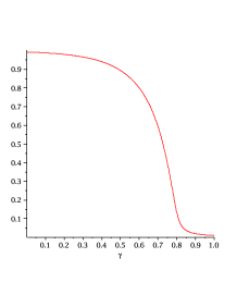
Figure 2: Function $h(\gamma)$ for strong protection as a function of $\gamma$; $\lambda=10$, $q^{+}=0.5$, $p=0.01$

As $\gamma$ the fraction of agents investing in protection increases, the incentive to invest in protection decreases. In fact, it is less attractive for an agent to invest in protection, should others then decide to do so. As more agents invest, the expected benefit of following suit decreases since there is a lower probability of loss, the network becoming more secure.

Weak protection: investing in protection does lower the probability of contagion $q$ but it remains positive: $0<q<q^{+}$. In this case, the map $\gamma\mapsto h(\gamma)$ can be non-decreasing for small value of $\gamma$ and decreasing for values of $\gamma$ close to one (see Figure 3).

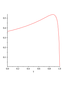
Figure 3: Function $h(\gamma)$ for weak protection as a function of $\gamma$; $\lambda=10$, $q^{+}=0.5$, $p^{+}=0.01$ and $q=0.1$

For small values of $\gamma$, the incentive for an agent to invest in security actually increases with the proportion of agents investing in security (recall Condition (8)). We will see in the next section, that this alignment of incentives is responsible for a coordination problem when agents are strategic.

III-C Sufficient conditions for monotone investment in a network

We now show how the condition (8) extends to a general framework. This extension is given by the following result:

Theorem 3.

If the function $p(x,v,\gamma)-p(x,v^{\prime},\gamma^{\prime})$ is strictly increasing in $x\in X$ for any $(v^{\prime},\gamma^{\prime})>(v,\gamma)$ and the function $p(x,v,\gamma)$ is non-increasing in $x$, then $\varphi(v,\ell,\gamma)$ defined in (6) is non-decreasing.

Proof.

As noticed in Remark 3, we need to prove that our condition ensures that $\ell p(x,v,\gamma)-\ell^{\prime}p(x,v^{\prime},\gamma^{\prime})$ is strictly increasing in $x\in X$ for any $(v^{\prime},\ell^{\prime},\gamma^{\prime})>(v,\ell,\gamma)$. If $\ell=\ell^{\prime}$, this follows from the condition of the theorem. We now deal with the case $\ell^{\prime}>\ell$. Let $x^{\prime}>x$, then by the condition of the theorem, we have

$$\ell p(x^{\prime},v,\gamma)-\ell p(x^{\prime},v^{\prime},\gamma^{\prime})>\ell p(x,v,\gamma)-\ell p(x,v^{\prime},\gamma^{\prime}),$$

but since $\ell^{\prime}>\ell$ and $p(x,v^{\prime},\gamma^{\prime})-p(x^{\prime},v^{\prime},\gamma^{\prime})\geq 0$ for $x^{\prime}>x$, we also have

$$\ell p(x^{\prime},v^{\prime},\gamma^{\prime})-\ell^{\prime}p(x^{\prime},v,^{\prime},\gamma^{\prime})>\ell p(x,v^{\prime},\gamma^{\prime})-\ell^{\prime}p(x,v^{\prime},\gamma^{\prime}).$$

Summing these inequalities gives exactly the desired result. ∎

Remark 4.

Clearly, the condition of Theorem 3 translates in the setting described in Section III-B to $p(0,\gamma)-p(0,\gamma^{\prime})<p(1,\gamma)-p(1,\gamma^{\prime}),\mbox{ for any }\gamma^{\prime}>\gamma$, which corresponds exactly to (8).

In the particular case where $\Gamma$ is a subset of $\mathbb{R}$, and under some smoothness conditions, we obtain:

Proposition 3.

If the function $p(x,v,\gamma)$ is twice continuously differentiable on $X\times[0,1]\times\Gamma$, then sufficient conditions for $\varphi(v,\ell,\gamma)$ to be non-decreasing are: $\frac{\partial p}{\partial x}(x,v,\gamma)\leq 0$, $\frac{\partial^{2}p}{\partial x\partial v}(x,v,\gamma)\leq 0$, $\frac{\partial^{2}p}{\partial x\partial\gamma}(x,v,\gamma)\leq 0$.

As we will see in the next section satisfying the conditions of Theorem 3 (or Proposition 3) ensures that the incentives in the population are aligned but this might lead to a coordination problem.

IV Equilibrium analysis of the security game

We now present our results in a game-theoretic framework where each agent is strategic. We assume that the effect of the action of any single agent is infinitesimal but each agent anticipates the effect of the actions of all other agents on the security level of the network.

IV-A Information structure and fulfilled expectations equilibrium

In most of the literature on security games, it is assumed that the player has complete information. In particular, each player knows the probability of propagation of the attack or failure from each other player in the network and also the cost functions of other players. In this case, the agent is able to compute the Nash equilibria of the games (if no constraint is made on the computing power of the agent) and decides on her level of investment accordingly. In particular, the agent is able to solve (6) for all possible values of $\gamma$ which capture the decision of all other agents. Note that even if only binary decisions are made by agents the size of the set $\Gamma$ grows exponentially with the number of players in the network. Moreover in a large network, the complete information assumption seems quite artificial, especially for security games where complete information would then implies that the agents disclose information on their security strategy to the public and hence to the potential attacker!

Here we relax the assumption of complete information. As in previous section, we assume that each agent is able to compute the function $p(x,v,\gamma)$ based on public information and on the epidemic risk model. The values of the possible loss $\ell$ and the vulnerability $v$ are private information of the agent and vary among the population. In order to define properly the equilibrium of the game, we assume that all players are strategic and are able to do this computation. Hence if a player expect that a fraction $\gamma^{e}$ of the population invests in security, she can decide for her own investment. We assume that at equilibrium expectations are fulfilled so that at equilibrium the actual value of $\gamma$ coincides with $\gamma^{e}$. This concept of fulfilled expectations equilibrium to model network externalities is standard in economics (see Section 3.6.2 in [5]).

We now describe it in more details. For simplicity of the presentation, we do not consider the dependence in the vulnerability $v$ since in the security game, we focus on the monotonicity in $\gamma$ which will turn out to be crucial. We also consider that the choice regarding investment is binary, i.e. $X=\{0,1\}$.

We consider a heterogeneous population, where agents differ in loss sizes only. This loss size $\ell$ is called the type of the agent. We assume that agents expect a fraction $\gamma^{e}$ of agents in state $S$, i.e. to make their choice, they assume that the fraction of agents investing in security is $\gamma^{e}$. We now define a network externalities function that captures the influence of the expected fraction of agents in state $S$ on the willingness to pay for security. Let the network externalities function be $h(\gamma^{e})$. More precisely, for an agent of type $\ell$, the willingness to pay for protection in a network with a fraction $\gamma^{e}$ of the agents in state $S$ is given by $\ell h(\gamma^{e})$ so that if

$$\ell h(\gamma^{e})\geq c,\mbox{ (where $c$ is the cost of the security option)}$$ (9)

the agent will invest and otherwise not. Hence (9) is in accordance with (7) (where the cost was normalized to one). Note that here, we do not make any a priori assumption on the network externalities function $h$ which can be general and fit to various models.

Indeed, our model corresponds exactly to the multiplicative formulation of Economides and Himmelberg [25] which allows different types of agents to receive differing values of network externalities from the same network. As explained above, agents with low $\ell$ have little or no use for the protection whereas agents with high $\ell$ value highly security. This is taken into account in our model since for a fixed expected fraction of agents in state $S$, agents with high $\ell$ have a higher willingness to pay for self-protection than agents with low $\ell$.

Let the cumulative distribution function of types be $F(\ell)$, i.e the fraction of the population having type lower than $\ell$ is given by $F(\ell)\leq 1$. We make the following hypothesis:

Hypothesis 1.

$F(\ell)$ is continuous with positive density everywhere on its support which is normalized to be $[0,1]$.

Note in particular that $F$ is strictly increasing and it follows that the inverse $F^{-1}(\gamma)$ is well-defined for $\gamma\in[0,1]$.

Given expectation $\gamma^{e}$ and cost for protection $c$, all agents with type $\ell$ such that $\ell h(\gamma^{e})>c$ will invest in protection. Hence the actual fraction of agents investing in protection is given by $\gamma=1-F\left(\min\left(\frac{c}{h(\gamma^{e})},1\right)\right)$. Hence following [25], we can invert this equation and we define the willingness to pay for the last agent in a network of size $\gamma$ with expectation $\gamma^{e}$ as

$$w(\gamma,\gamma^{e})=h(\gamma^{e})F^{-1}(1-\gamma).$$ (10)

Seen as a function of its first argument, this is just an inverse demand function: it maps the quantity of protection demanded to the market price. Because of externalities, expectations affect the willingness to pay:

$$\frac{\partial w}{\partial\gamma^{e}}(\gamma,\gamma^{e})=h^{\prime}(\gamma^{e})F^{-1}(1-\gamma).$$ (11)

For goods that do not exhibit network externalities, demand slopes downward: as price increases, less of the good is demanded. This fundamental relationship may fail in goods with network externalities. If $h^{\prime}(.)>0$, then the willingness to pay for the last unit may increase as the number expected to be sold increases as can be seen from (11): $\frac{\partial w}{\partial\gamma^{e}}(\gamma,\gamma^{e})>0$. For example in [25] studying the FAX market, as more and more agents buy a FAX, the utility of the FAX increases since more and more agents can be reached by this communication mean. For a fixed cost $c$, in equilibrium, the expected fraction $\gamma^{e}$ and the actual one $\gamma$ must satisfy

$$c=w(\gamma,\gamma^{e})=h(\gamma^{e})F^{-1}(1-\gamma).$$ (12)

If we assume moreover that in equilibrium, expectations are fulfilled, then the possible equilibria are given by the fixed point equation:

$$c=w(\gamma,\gamma)=h(\gamma)F^{-1}(1-\gamma)=:w(\gamma).$$ (13)

We see that if $h^{\prime}(.)>0$, the concept of fulfilled expectations equilibrium captures the possible increase in the willingness to pay as the number expected to be sold increases. This would corresponds to the case where we have $w^{\prime}(\gamma)>0$ for some values of $\gamma$. In such cases, a critical mass phenomenon (as in the FAX market [25]) can occurs : there is a problem of coordination. We explain this phenomenon more formally in the next section and then show how our results differ from [25]. We end this section with the following important remark:

Remark 5.

The case of an homogeneous population in which all agents have the same type, i.e the same loss size $\ell$ corresponds to the function $F^{-1}$ being constant equal to $\ell$. In this case, the willingness to pay is simply $w(\gamma)=h(\gamma)\ell$. In particular, the epidemic risk model presented above can be used to model the network externalities by the function $h(\gamma)$ computed in Section III. In this case, Condition (8) still gives a condition for incentives to be align. As we will see next, this condition might lead to critical mass: if incentives are aligned, there is a coordination problem!

IV-B Critical mass: coordination problem

To determine the possible equilibria, we analize the shape of the fulfilled expectations demand $w(\gamma)$. First we have $w(0)\geq 0$ which is equal to the value of the self-protection assuming there are no network externalities. We also have $w(1)=0$ since by Hypothesis 1, we have $F^{-1}(0)=0$. In words, this means that there are agents with very low $\ell$ who have little or no interest in self-protection. Then in order to secure completely the network, we have to convince even agents of very low willingness to pay.

The slope of the fulfilled expectations demand is

$$w^{\prime}(\gamma)=-\frac{h(\gamma)}{F^{\prime}(F^{-1}(1-\gamma))}+h^{\prime}(\gamma)F^{-1}(1-\gamma).$$ (14)

The first term measures the slope of the inverse demand without taking into account the effect of the expectations. The second term corresponds to the effect of an increase in the expected fraction of agents in state $S$. If $h^{\prime}(.)>0$ as in [25], it corresponds to the increase in the willingness to pay of the last agent investing in self-protection created by his own action in joining the group of agents in state $S$. Note that in any case, if the fraction of agents in state $S$ gets very large, i.e. $\gamma\to 1$, the last agent investing in self-protection has very low willingness to pay for it. Hence for $\gamma$ close to one, the effect of marginal expectations on the marginal agent investing in $S$ is negligible. Formally this is observed by $\lim_{\gamma\to 1}h^{\prime}(\gamma)F^{-1}(1-\gamma)=0$. It follows that

$$\lim_{\gamma\to 1}w^{\prime}(\gamma)=\lim_{\gamma\to 1}-\frac{h(\gamma)}{F^{\prime}(F^{-1}(1-\gamma))}=-\frac{h(1)}{F^{\prime}(0)}<0.$$ (15)

Note that we allow $F^{\prime}(0)=0$ in which case, Equation (15) should be interpreted as $\lim_{\gamma\to 1}w^{\prime}(\gamma)=-\infty$. The sign of $\lim_{\gamma\to 0}w^{\prime}(\gamma)$ depends on the parameters of the model and we will see that it is of crucial importance. We make the following hypothesis

Hypothesis 2.

The function $w(\gamma)$ is single-peaked.

Note that in the case of an homogeneous population, $w(\gamma)=h(\gamma)\ell$, where $h(\gamma)$ was computed in Section III for the epidemic risk model and is single-peaked.

We are now ready to state the main result of this section:

Theorem 4.

Under Hypothesis 1 and 2, a network has positive critical mass if $\lim_{\gamma\to 0}h^{\prime}(\gamma)>0$ and either

• $w(0)=0$, i.e. if all agents are in state $N$ then no agent is willing to invest in self-protection;

• $\lim_{\gamma\to 0}h^{\prime}(\gamma)$ is sufficiently large, i.e. there are large private benefits to join the group of agents in state $S$ when the size of this group is small;

• $\lim_{\gamma\to 1}F^{\prime}(\gamma)$ is sufficiently large, i.e. there is a significant density of agents who are ready to invest in self-protection even if the number of agents already in state $S$ is small.

Remark 6.

Note that if $h^{\prime}(\gamma)>0$ for small values of $\gamma$, then incentives are aligned by results of previous Section but this might lead to a coordination problem. Indeed as shown by previous theorem, this is a necessary condition for a network to exhibit positive critical mass. In the case of a homogeneous population (see Remark 5), the function $w(\gamma)$ is proportional to the function $h(\gamma)$ computed in Section III for the epidemic risk model. In particular, in the case of weak protection, there is positive critical mass as shown by Figure 3.

Proof.

Since we proved that $\gamma\mapsto w(\gamma)$ is decreasing for $\gamma$ close to one, there are only two possibilities: either is is increasing for small values of $\gamma$ or it is decreasing for all $\gamma$. As explained in Lemma 1 of [25], the network has a positive critical mass if and only if $\gamma\mapsto w(\gamma)$ is increasing for small values of $\gamma$.

\psfrag{pi}{$c$}\psfrag{pi0}{$c_{0}$}\psfrag{gam}{$\gamma$}\psfrag{gami}{$\gamma_{i}$}\psfrag{gams}{$\gamma_{s}$}\psfrag{gam0}{$\gamma_{0}$}\includegraphics[angle={0},width=113.81102pt]{dem.eps}

Figure 4: Willingness to pay curve (or demand curve) $w(\gamma)$

This is illustrated thanks to Figure 4 (which should be compared to Figure 3). Recall that in equilibrium, we have $w(\gamma^{*})=h(\gamma^{*})F^{-1}(1-\gamma^{*})=c$. If we imagine a constant cost $c$ decreasing parametrically, the network will start at a positive and significant size $\gamma^{0}$ corresponding to a cost $c^{0}$. For each smaller cost $c^{1}<c<c^{0}$, there are three values of $\gamma^{*}$ consistent with $c$: $\gamma^{*}=0$; an unstable value of $\gamma^{*}$ at the first intersection of the horizontal through $c$ with $w(\gamma)$; and the Pareto optimal stable value of $\gamma^{*}$ at the largest intersection of the horizontal with $w(\gamma)$.

As explained above, a network exhibits a positive critical mass if and only if $\lim_{\gamma\to 0}w^{\prime}(\gamma)>0$. Now by (14), we have $\lim_{\gamma\to 0}w^{\prime}(\gamma)=\lim_{\gamma\to 0}h^{\prime}(\gamma)-\frac{h(0)}{\lim_{\gamma\to 1}F^{\prime}(\gamma)}$, note that $h(0)=w(0)$ and the theorem follows easily. ∎

We finish this section by explaining the main difference between our model and models with standard positive externalities. Informally, in the model of [25] for the FAX market, when a new agent buys the good (a FAX machine), he has a personal benefit and he also increases the value of the network of FAX machines. This is a positive externality which are felt only by the adopters of the good. Indeed, when this agent buys the good, this is a negative externality on the agents who did not buy the good (see [26], Example A9 in [17]). In our case, when an agent chooses to invest in security, the externalities are always positive and we have to distinguish between two positive externalities: one is felt by the agents in state $S$ and the other is felt by the agent in state $N$. Indeed as $\gamma$ increases, both populations experience a decrease of their probability of loss but the value of this decrease is not the same in both populations. We call the ’public externalities’ the decrease felt by agents in state $N$ and it is given by $g(\gamma)=p(0,0)-p(0,\gamma)\geq 0$. We call the ’private externalities’ the decrease felt only by agents in state $S$ and it is given by $g(\gamma)+h(\gamma)=p(0,0)-p(1,\gamma)\geq g(\gamma)$.

First note that the notations are consistent. In particular, Equation (9) still gives the willingness to pay for self-protection in a network with a fraction $\gamma^{e}$ of the agents in state $S$. We are still dealing with positive externalities, however this does not imply that $h^{\prime}(.)>0$ (as it is the case in [25]). Instead, positive externalities (i.e. the fact that both the public externalities $g(\gamma)$ and the private externalities $g(\gamma)+h(\gamma)$ are increasing in $\gamma$) only ensures that:

$$g^{\prime}(.)\geq 0\mbox{ and, }g^{\prime}(.)+h^{\prime}(.)\geq 0.$$ (16)

Assumption (16) ensures the sensible fact that the more agents invest in self-protection, the more secure the network becomes (this is the total effect). If in addition, $h^{\prime}(.)\geq 0$, then adoption of security increases others’ incentive to invest (this is the marginal effect) and there might be a critical mass effect. Recent works on the marginal effect include Segal’s increasing externalities [17] or Topkis’supermodularity [18]. On the contrary when $h^{\prime}(.)<0$, there is no coordination problem (no critical mass). However, we show in the next section that even in this case, the equilibrium is not socially efficient. The intuition for this fact is that incentives are not anymore aligned and since agent benefits from the investment in security of the other agents, they prefers to ’free-ride’ the investment of the other agents.

IV-C Welfare Maximization

A planner who maximizes social welfare can fully internalize the network externalities and this is the situation we now consider. We will show that there is always efficiency loss in our model with exogenous price. In other words, the price of anarchy is always greater than one.

Theorem 5.

Under Hypothesis 1 and 2, a social planner will choose a larger fraction $\gamma$ of agents investing in self-protection than the market equilibrium for any fixed cost $c$.

We refer to [8] for an estimate of this price of anarchy for the epidemic risks model presented in previous section and to [24] for an extension to graphs with power-law degrees distribution.

Proof.

The social welfare function is:

$$W(\gamma) = g(\gamma)\int_{\gamma}^{1}F^{-1}(1-u)du$$

$$+ \left(g(\gamma)+h(\gamma)\right)\int_{0}^{\gamma}F^{-1}(1-u)du-c\gamma,$$

where $g(\gamma)\int_{\gamma}^{1}F^{-1}(1-u)du$ is the gross benefit for the fraction of agents in state $N$ and $\left(g(\gamma)+h(\gamma)\right)\int_{0}^{\gamma}F^{-1}(1-u)du$ for the fraction of agents in state $S$ and $c\gamma$ are the costs. We denote by $B(\gamma)$ the gross benefit for the whole population so that $W(\gamma)=B(\gamma)-c\gamma$, then we have:

$$B^{\prime}(\gamma) = h(\gamma)F^{-1}(1-\gamma)$$

$$= +\left(h^{\prime}(\gamma)+g^{\prime}(\gamma)\right)\int_{0}^{\gamma}F^{-1}(1-u)du$$

$$+ g^{\prime}(\gamma)\int_{\gamma}^{1}F^{-1}(1-u)du.$$

Recall that by (12), the equilibria of the game (without the social planner) are the values $\gamma$ such that $w(\gamma)=h(\gamma)F^{-1}(1-\gamma)=c$. In particular for such a value of $\gamma$, since we assume positive externalities (16), we have that $B^{\prime}(\gamma)\geq w(\gamma)=c$, hence $W^{\prime}(\gamma)\geq 0$ and the theorem follows. ∎

V Conclusion

In this paper, we study under which conditions agents in a large network invest in self-protection. We started our analysis with finding conditions when the amount of investment increases for a single agent as the vulnerability and loss increase. We also showed that risk-neutral agent do not invest more than 37% of the expected loss under log-convex security breach probability functions. We then extended our analysis to the case of interconnected agents of a large network using a simple epidemic risk models. We derived a sufficient condition on the security breach probability functions taking into consideration the global knowledge on the security of the entire network for guaranteeing increasing investment with increasing vulnerability. It would be interesting to use other epidemics models as in [27] to see the impact on the results of this section.

Finally, we study a security game where agents anticipate the effect of their actions on the security level of the network. We showed that in all cases, the fulfilled equilibrium is not socially efficient. We explained it by the separation of the network externalities in two components: one public (felt by agents not investing) and the other private (felt only by agents investing in self-protection). We also showed that alignment of incentives typically leads to a coordination problem.

In view of our results, it would be interesting to derive sufficient conditions for non-alignment of the incentives as these conditions would ensure that there is no coordination problem. Exploring this issue is an interesting open problem. Another interesting direction of research concerns the information structure of such games. For example, in the case presented here of epidemic risk model, what is the impact of an error in the estimation of the contagion probability which could be for example over evaluated by the firm selling the security solution? Also, in our work, the attacker is not a strategic player: attacks are made at random with probability of success depending of the security level of the agent targeted. However if the attacker can observe the security policies taken by the defenders, it can exploit this information [28]. An interesting extension would be to incorporate in our model such a strategic attacker as in [29]. Another extension could also consider the supply side, i.e. the firms distributing the security solution in the population. Very basic cases have been studied [30, 31] but again with a non strategic attacker.

References

- [1] M. Lelarge, “Coordination in network security games,” in INFOCOM, A. G. Greenberg and K. Sohraby, Eds. IEEE, 2012, pp. 2856–2860.
- [2] R. Anderson, “Why information security is hard-an economic perspective,” in ACSAC ’01: Proceedings of the 17th Annual Computer Security Applications Conference. Washington, DC, USA: IEEE Computer Society, 2001, p. 358.
- [3] R. Anderson and T. Moore, “Information security economics - and beyond,” Working Papers, 2008.
- [4] M. J. van Eeten and J. M. Bauer, “Economics of malware: Security decisions, incentives and externalities,” OECD Directorate for Science, Technology and Industry, OECD Science, Technology and Industry Working Papers 2008/1, May 2008. [Online]. Available: http://ideas.repec.org/p/oec/stiaaa/2008-1-en.html
- [5] J. Farrell and P. Klemperer, Coordination and Lock-In: Competition with Switching Costs and Network Effects, ser. Handbook of Industrial Organization. Elsevier, 2007, vol. 3, ch. 31, pp. 1967–2072.
- [6] H. R. Varian, “System reliability and free riding,” in in Economics of Information Security, Kluwer 2004 pp 1–15. Kluwer Academic Publishers, 2002, pp. 1–15.
- [7] H. Kunreuther and G. Heal, “Interdependent security,” Journal of Risk and Uncertainty, vol. 26, no. 2-3, pp. 231–49, March-May 2003.
- [8] M. Lelarge and J. Bolot, “Network externalities and the deployment of security features and protocols in the internet,” in SIGMETRICS ’08. New York, NY, USA: ACM, 2008, pp. 37–48.
- [9] J. Grossklags, N. Christin, and J. Chuang, “Security investment (failures) in five economic environments: A comparison of homogeneous and heterogeneous user agents,” WEIS, 2008.
- [10] L. Jiang, V. Anantharam, and J. Walrand, “How bad are selfish investments in network security?” Networking, IEEE/ACM Transactions on, vol. 19, no. 2, pp. 549 –560, april 2011.
- [11] R. A. Miura-Ko, B. Yolken, J. Mitchell, and N. Bambos, “Security decision-making among interdependent organizations,” in CSF ’08: Proceedings of the 2008 21st IEEE Computer Security Foundations Symposium. Washington, DC, USA: IEEE Computer Society, 2008, pp. 66–80.
- [12] J. Omic, A. Orda, and P. Van Mieghem, “Protecting against network infections: A game theoretic perspective,” in IEEE INFOCOM, 2009.
- [13] L. Gordon and M. Loeb, “The economics of information security investment,” ACM transactions on information and system security, vol. 5, no. 4, pp. 438–457, 2002.
- [14] M. Lelarge, “Economics of malware: Epidemic risks model, network externalities and incentives,” in Allerton, 2009.
- [15] B. Johnson, J. Grossklags, N. Christin, and J. Chuang, “Uncertainty in interdependent security games,” in Decision and Game Theory for Security, ser. Lecture Notes in Computer Science, T. Alpcan, L. Buttyán, and J. Baras, Eds., 2010, vol. 6442, pp. 234–244.
- [16] G. Theodorakopoulos, J.-Y. L. Boudec, and J. S. Baras, “Selfish response to epidemic propagation,” CoRR, vol. abs/1010.0609, 2010.
- [17] I. Segal, “Contracting with externalities,” The Quarterly Journal of Economics, vol. 114, no. 2, pp. 337–388, may 1999.
- [18] D. M. Topkis, Supermodularity and complementarity, ser. Frontiers of Economic Research. Princeton, NJ: Princeton University Press, 1998.
- [19] J. Bolot and M. Lelarge, “A New Perspective on Internet Security using Insurance,” in IEEE INFOCOM, 2008, pp. 1948–1956.
- [20] ——, “Cyber Insurance as an Incentive for Internet Security,” in Workshop in Economics of Information Security (WEIS) Seventh Workshop on Economics of Invormation Security, June, 2008, pp. 25–28.
- [21] M. Lelarge and J. Bolot, “Economic Incentives to Increase Security in the Internet: The Case for Insurance,” in IEEE INFOCOM, 2009.
- [22] D. M. Topkis, “Minimizing a submodular function on a lattice,” Operations Res., vol. 26, no. 2, pp. 305–321, 1978.
- [23] R. Durrett, Random graph dynamics, ser. Cambridge Series in Statistical and Probabilistic Mathematics. Cambridge: Cambridge University Press, 2007.
- [24] M. Lelarge and J. Bolot, “A local mean field analysis of security investments in networks,” in NetEcon ’08. New York, NY, USA: ACM, 2008, pp. 25–30.
- [25] N. Economides and C. Himmelberg, “Critical mass and network size with application to the us fax market,” New York University, Leonard N. Stern School of Business, Department of Economics, Working Papers 95-11, Aug. 1995.
- [26] M. L. Katz and C. Shapiro, “Network externalities, competition, and compatibility,” American Economic Review, vol. 75, no. 3, pp. 424–40, June 1985.
- [27] M. Lelarge, “Diffusion and cascading behavior in random networks,” Games and Economic Behavior, vol. 75, no. 2, pp. 752–775, 2012.
- [28] Z. Chen and C. Ji, “Optimal worm-scanning method using vulnerable-host distributions,” IJSN, vol. 2, no. 1/2, pp. 71–80, 2007.
- [29] Y. Bachrach, M. Draief, and S. Goyal, “Security games with contagion,” Tech. Rep., 2011.
- [30] M. Lelarge, “Efficient control of epidemics over random networks,” in SIGMETRICS/Performance, J. R. Douceur, A. G. Greenberg, T. Bonald, and J. Nieh, Eds. ACM, 2009, pp. 1–12.
- [31] C. Borgs, J. Chayes, A. Ganesh, and A. Saberi, “How to distribute antidote to control epidemics.”