A rapidly converging domain decomposition method for the Helmholtz equation

Abstract

A new domain decomposition method is introduced for the heterogeneous 2-D and 3-D Helmholtz equations. Transmission conditions based on the perfectly matched layer (PML) are derived that avoid artificial reflections and match incoming and outgoing waves at the subdomain interfaces. We focus on a subdivision of the rectangular domain into many thin subdomains along one of the axes, in combination with a certain ordering for solving the subdomain problems and a GMRES outer iteration. When combined with multifrontal methods, the solver has near-linear cost in examples, due to very small iteration numbers that are essentially independent of problem size and number of subdomains. It is to our knowledge only the second method with this property next to the moving PML sweeping method.

1 Introduction

In this paper we introduce a new domain decomposition method for the solution of the Helmholtz equation in two and three dimensions. To be specific we consider in 2-D

$$-\partial_{xx}^{2}u(x,y)-\partial_{yy}^{2}u(x,y)-k(x,y)^{2}u(x,y)=f(x,y),$$ (1)

where $k(x,y)=\frac{\omega}{c(x,y)}$, with $c(x,y)$ the wave speed. The computational domain is assumed to be a rectangle that is truncated using the perfectly matched layer [1]. We focus on solving the large linear systems resulting from discretization with standard 5 or 7 point finite differences.

We have two main findings. First, we have constructed new transmission conditions. These are designed to ensure that

(i) the boundary conditions at the subdomain interfaces are non-reflecting; (ii) if $$\Omega_{j-1} \Omega_{j} \Omega_{j-1} \Omega_{j}$$ and are neighboring subdomains then the outgoing wave field from equals the incoming wave field in at the joint boundary and vice versa. (2)

This is achieved in a simple and accurate way using PML boundary layers added to the subdomains and single layer potentials. See [2] for a related approach in the finite element discretization of the time harmonic Maxwell equations.

Our most remarkable finding concerns the situation where the domain is split into many thin layers along one of the axes, say $J$ subdomains numbered from 1 to $J$. Following [3] we will also call these quasi 2-D subdomains. Generally, an increase in the number of subdomains leads to an increase in the number of iterations required for convergence. Here we propose and study a method where the number of iterations is essentially independent of the number of subdomains.

A necessary condition for this is that information can travel over the entire domain (or at least an $O(1)$ part thereof) in one iteration. To achieve this we use a multiplicative method, where the subdomains are first solved consecutively from $j=1$ to $j=J$, each time using information from the solution of the neighboring, previously solved subdomain, and then in the same way from $j=J$ downto $j=1$ using the residual as right hand side. In this way information can travel all over the domain with only two solves per subdomain. The procedure is used as a preconditioner for GMRES.

We studied numerically the convergence of the method for different choices of the grid distance $h$ and the frequency $\omega$, keeping $\omega h$ constant, and different numbers of subdomains. In our examples the method converged rapidly, with generally less than 10 iterations needed for reduction of the residual by $10^{-6}$. Moreover, the required number of iterations was essentially independent of the size of the domain and the number of subdomains.

This is attractive in combination with the use of multifrontal methods for the subdomain solves. Indeed, as was argued by Engquist and Ying [3], in 3-D the set of quasi 2-D subproblems can be solved by multifrontal methods in $O(N\log N)$ time, with $O(N^{4/3})$ cost for the factorization, versus $O(N^{3/2})$ and $O(N^{2})$ when the multifrontal method is applied directly to the 3-D system. The method therefore behaves near-linearly. It is the second such method we are aware of, in addition to the moving PML sweeping method, for which such observations were made in [3].

Several things have to be kept in mind. First, we estimate, based on our examples, that the thickness of the PML layers needs to increase with increasing $N$. A required growth of $O(\log N)$ is consistent with our data. This would lead to an additional factor $O(\log N)$ for the cost of the solves and $O((\log N)^{2})$ for the cost of the preparation. Secondly, the method is only near-linear provided that solutions are required for a sufficiently large number of right hand sides to recoup the cost of the factorization. Thirdly, because of the multiplicative way of domain decomposition, the method is not in itself parallel. In section 5 two solutions for this problem are discussed. Finally, numerical tests have shown that for cavities, the claimed results do not hold. (Indeed, the cavity problem is known to be especially difficult for iterative methods because of the many near-zero eigenvalues.)

1.1 The method and its context

Next we discuss in more detail the ideas behind the method and some of the relevant literature.

To motivate our approach we recall the 1-D problem with $k=\text{constant}$, see the review in [4] or [5, 6, 7]. Let $]0,L[$ be the domain. The differential equation and the Robin boundary conditions read

$$-\partial^{2}_{xx}u(x)-k^{2}u(x)={} f(x) \text{for $0<x<L$},$$

$$\partial_{x}u+iku={} 0 x=0$$ at

$$-\partial_{x}u+iku={} 0 x=L$$ at .

The Robin boundary conditions are exact non-reflecting boundary conditions and ensure that there are no incoming waves at the boundaries. We assume the domain is divided in $J$ subdomains $]b_{j-1},b_{j}[$ with

$$0=b_{0}<b_{1}<\ldots<b_{J}=L.$$

The original problem is then equivalent to $J$ subdomain problems with continuity conditions at the interfaces as follows

$$-\partial_{xx}^{2}u^{(j)}-k^{2}u^{(j)}={} f^{(j)} \text{for }x\in]b_{j-1},b_{j}[$$

$$\partial_{x}u^{(j)}+iku^{(j)}={} \partial_{x}u^{(j-1)}+iku^{(j-1)} \text{at }x=b_{j-1}$$

$$-\partial_{x}u^{(j)}+iku^{(j)}={} -\partial_{x}u^{(j+1)}+iku^{(j+1)} \text{at }x=b_{j}$$

(by convention $u^{(0)}=0=u^{(J+1)}$). These continuity conditions satisfy the property (2). To obtain an iterative solution method, the right hand side of the continuity conditions is taken from the previous iteration, i.e. a sequence $v_{n}^{(j)}$ is constructed, where $n$ is the iteration number and $j$ the subdomain index according to

$$-\partial_{xx}^{2}v_{n}^{(j)}-k^{2}v_{n}^{(j)}={} f^{(j)} \text{for }x\in]b_{j-1},b_{j}[$$ (3)

$$\partial_{x}v_{n}^{(j)}+ikv_{n}^{(j)}={} \partial_{x}v_{n-1}^{(j-1)}+ikv_{n-1}^{(j-1)}, \text{at }x=b_{j-1}$$ (4)

$$-\partial_{x}v_{n}^{(j)}+ikv_{n}^{(j)}={} -\partial_{x}v_{n-1}^{(j+1)}+ikv_{n-1}^{(j+1)} \text{at }x=b_{j}.$$ (5)

This method is optimal in the sense that it converges in a finite number, namely $J$, of iterations. Indeed, recall that the solution for the problem $-\partial_{xx}^{2}u(x)-k^{2}u(x)=f(x)$ with Robin boundary conditions $\partial_{x}u(0)+iku(0)=h_{1}$, $-\partial_{x}u(L)+iku(L)=h_{2}$ is given by

$$u(x)=\frac{i}{2k}\int_{0}^{x}e^{ik(x-s)}f(s)\,ds+\frac{i}{2k}\int_{x}^{L}e^{-ik(x-s)}f(s)\,ds+\frac{e^{ikx}}{2ik}h_{1}+\frac{e^{-ik(x-L)}}{2ik}h_{2}$$ (6)

It follows by induction, starting from $v_{0}^{(j)}=0$, that $v_{n}^{(j)}$ satisfies

$$v_{n}^{(j)}(x)=\frac{i}{2k}\int_{A}^{x}e^{ik(x-s)}f(s)\,ds+\frac{i}{2k}\int_{x}^{B}e^{-ik(x-s)}f(s)\,ds$$

where $A=b_{\max(0,j-n)}$ and $B=b_{\min(J,j+n-1)}$. After $J$ steps, $A=0$ and $B=L$ for all $j\in\{1,\ldots,J\}$.

This work answers two questions about the iterative method (3)-(5). The first question concerns the generalization of the transmission conditions to two and three dimensions. The Robin boundary conditions then no longer satisfies the properties (2) (see the argument around (24) below). Several approaches have been proposed in the literature. First, the Robin boundary conditions can still be used as transmission conditions [8]. Several authors have also considered optimized Robin transmission conditions [9, 10]. A second possible approach involves operator valued Robin boundary conditions [11] and ideas about numerical absorbing boundary conditions, e.g. [12]. Padé approximations for $\lambda$ in (27) (see below) can be used to obtain numerical absorbing boundary and transmission conditions [13, 14]. In this paper we use PML boundary layers [1] to achieve (2). Earlier work using domain decomposition with PML’s is in [15] and in [2] (cf. the discussion in section 5).

The second question concerns the case of large $J$. In one iteration of (3)-(5) information from one subdomain can only travel to its neighbors. The method therefore requires at least $O(J)$ iterations to converge, hence $O(J^{2})$ subdomain solves. On the other hand, by using the multiplicative approach outlined below, solving the subdomains consecutively, first $j=1,2,\ldots,J$, and then $j=J,J-1,\ldots,1$, information can travel over the full domain in just $2$ solves per subdomain. Here we will follow this multiplicative approach.

As mentioned, the case of a large number of thin layers, say $k$ grid points thick, is of interest when the method is used in combination with multifrontal methods for the subdomain solves.The computational cost of such a setup was analyzed by Engquist and Ying [3], using results of [16]. Consider a cube with $n\times n\times n$ gridpoints, hence $N=n^{3}$. The cost of a $LU$ decomposition of a subdomain of the form $n\times n\times k$ is $O(k^{3}n^{3})$, while the cost of a backsubstition is $O(k^{2}n^{2}\log n)$. Assuming $k=O(1)$, the total cost of the factorizations is $O(N^{4/3})$, while the total cost per iteration is $O(N\log N)$. If the number of iterations depends weakly on problem size, as we see in examples, then this method scales well. In the presence of PML layers that have a thickness of $w_{\rm pml}$ grid points, a value $k\approx 4w_{\rm pml}$ is optimal for the thickness of the subdomains including PML layers, i.e. minimizes the cost of applying one set of subdomain solves. The details of our method will be explained in section 2.

The papers [17, 18] provide a review of solution methods for the Helmholtz equation. Some recent other work is given in [19, 20].

1.2 Results

Our first main result is a theoretical result, concerning the constant coefficient problem on a strip. Assuming that the PML layers perfectly reproduce the behavior of the solution on the unbounded domain, the methods solves this problem in one iteration, i.e. in one upward and one downward sequence of solves. We observe that the upward and downward sequence of solves can in fact be performed simultaneously, if the point where the the sequences cross is handled carefully.

The second main result is the good convergence behavior in numerical examples that was already mentioned in the first part of this introduction. In addition a comparison with a double sweep method with Robin transmission conditions was made. For small $J$ this can be attractive, but this method did not have near-linear cost like the PML-based method.

1.3 Contents

The paper is organized as follows. The next section explains in detail our method. Section 3 contains some theoretical results. Then in section 4 the numerical examples are discussed. We end the paper with a short discussion.

2 The method

2.1 Continuous formulation

In this section we formulate our method in 2-D. The domain is assumed to be a set of the form $\Omega=]0,L[\times]0,1[$. It is straightforward to generalize this to rectangular domains of different size, and to 3-D rectangular domains.

The Helmholtz operator will be referred to as $A$, given away from the PML boundary layers by

$$A=-\partial^{2}_{xx}-\partial^{2}_{yy}-k(x,y)^{2}.$$

The operator in a PML layer at a boundary, say $x=\text{constant}$, is obtained by replacing

$$\frac{\partial}{\partial x}\rightarrow\frac{1}{1+i\frac{\sigma_{x}(x)}{\omega}}\frac{\partial}{\partial x}$$

where $\sigma_{x}=0$ in the interior of the domain, and positive inside the PML layers [21, 22].

The domain is divided into $J$ subdomains along the $x$-axis. The interface locations will be denoted by $x=b_{j}$, where

$$0=b_{0}<\ldots<b_{J}=L$$

The “core” subdomains, without additional PML layers, will be denoted by $D^{(j)}=]b_{j-1},b_{j}[\times]0,1[$. With PML layers added the notation $\Omega^{(j)}$ will be used. The latter sets are obtained by padding the $D^{(j)}$ with PML layers of size $L_{\rm pml}$ at the internal boundaries, i.e.

$$\Omega^{(j)}=]b_{j-1}-L_{\rm PML}(1-\delta_{j,1}),b_{j}+L_{\rm PML}(1-\delta_{j,J})[\times]0,1[$$

On the domains $\Omega^{(j)}$, functions $k^{(j)}(x,y)$ are defined that agree with $k$ on $D^{(j)}$, and are independent of $x$ and equal to $k$ at the boundary of the core subdomain inside the added PML layers, i.e.

$$k^{(j)}(x,y)=\left\{\begin{array}[]{ll}k(x,y)&\text{for $b_{j-1}\leq x\leq b_{j}$}\\ k(b_{j-1},y)&\text{for $x<b_{j-1}$ (if $j>1$)}\\ k(b_{j},y)&\text{for $x>b_{j}$ (if $j<J$).}\end{array}\right.$$

On the domains $\Omega^{(j)}$ operators $A^{(j)}$ are defined as Helmholtz operators with PML modifications, similar as $A$ was defined on $\Omega$.

Next we consider the approximation by domain decomposition of a solution $u$ to the 2-D Helmholtz equation $Au=f$. The function $f$ is assumed to be integrable, which allows the definition of $f^{(j)}$ on $\Omega^{(j)}$ by

$$f^{(j)}=\left\{\begin{array}[]{ll}f(x)&\text{if $x\in D^{(j)}$}\\ 0&\text{otherwise}\end{array}\right.$$

A first set of subdomain solutions $v^{(j)}$ is obtained by solving the equations

$$A^{(j)}v^{(j)}=f^{(j)}-2\delta(x-b_{j-1})\partial_{x}v^{(j-1)}(b_{j-1},\cdot),$$ (7)

consecutively for $j=1,2,\ldots,J$. Here by convention $v^{(0)}=0$. A function $v$ on $\Omega$ is then defined by

$$v(x,y)=v^{(j)}(x,y)\qquad\text{with $j$ s.t.\ $b_{j-1}<x<b_{j}$.}$$ (8)

The second term in the right hand side of (7) requires some explanation. While this is mostly done in the next section, a short intuitive explanation goes as follows. The term $v^{(j-1)}(b_{j-1},\cdot)$ exclusively contains forward going waves because of the presence of a PML non-reflecting layer immediately to its right in $\Omega^{(j)}$. The term $-2\delta(x-b_{j-1})\partial_{x}v^{(j-1)}(b_{j-1},\cdot)$ is meant to cause the same forward going wave field in the field $v^{(j)}$. The form of this term can be explained by the properties of the single layer potential. The solution to

$$Au=h(y)\delta(x-b_{j-1})$$

has the property that

$$\lim_{\epsilon\rightarrow 0}\partial_{x}u(b_{j-1}+\epsilon,y)-\partial_{x}u(b_{j-1}-\epsilon,y)=-h(y),$$

if $k$ is continuous at $x=b_{j-1}$. Assuming the medium $k^{(j)}$ is independent of $x$, the source $h(y)\delta(x-b_{j-1})$ generates waves propagating both forwardly and backwardly in a symmetric fashion. The factor $-2$ is introduced so that the forward propagating part equals $v^{(j-1)}(b_{j-1},y)$. The backward propagating part is absorbed in the neighboring PML layer. Note that in this way, all the subdomain sources $f^{(k)}$ with $k\leq j$ can contribute to the field $v^{(j)}$.

The downward sequence of subdomain solves takes as right hand side the restrictions to a subdomain of the residual

$$g=f-Av$$

However, $v$ is undefined and generally discontinuous at the boundaries $x=b_{j}$, $j=1,\ldots,J-1$. While $g$ is still well defined, it only exists as a generalized function (distribution), with most singular term of the form $\delta^{\prime}(x-b_{j})h(y)$.

The problem with this is not that $g$ is unsuitable as a right hand side. Solutions to Helmholtz equations with distributional right hand sides in general exist. And, as a Helmholtz equation is formally an elliptic equation, the solutions are smooth away from the singular support of the right hand side. However, the restriction of $g$ to the subdomains $D^{(j)}$ is not well defined. Indeed, such a restriction is obtained by multiplying $g$ by the indicator function $I_{D^{(j)}}$ of $D^{(j)}$, and this multiplication is in general not well defined, because of the overlapping singular supports.

Therefore we introduce a second set of domain boundaries

$$0=\tilde{b}_{0}<\tilde{b}_{1}<\ldots<\tilde{b}_{\tilde{J}}=L.$$

with $\tilde{b}_{j}\neq b_{k}$ for all $0<j<\tilde{J}$ and $0<k<J$. Similarly as above we defined sets $\tilde{D}^{(j)}$ and $\tilde{\Omega}^{(j)}$, by $\tilde{D}^{(j)}=]\tilde{b}_{j-1},\tilde{b}_{j}[\times]0,1[$, and $\tilde{\Omega}^{(j)}=]\tilde{b}_{j-1}-L_{\rm PML}(1-\delta_{j,1}),\tilde{b}_{j}+L_{\rm PML}(1-\delta_{j,J})[\times]0,1[$, and we let $\tilde{A}^{(j)}$ be the Helmholtz operator with PML modification on $\tilde{\Omega}^{(j)}$. The function $g^{(j)}$ on $\tilde{\Omega}^{(j)}$ can now be defined by

$$g^{(j)}(x,y)=I_{\tilde{D}^{(j)}}g(x,y).$$

Next a series of functions $w^{(j)}$ on $\tilde{\Omega}^{(j)}$ is determined for $j=\tilde{J},\tilde{J}-1,\ldots,1$ (computed in this order) from the equations

$$\tilde{A}^{(j)}w^{(j)}=g^{(j)}+2\delta(x-\tilde{b}^{(j)})\partial_{x}w^{(j+1)}(\tilde{b}_{j},\cdot),$$ (9)

and a function $w$ is defined by

$$w(x,y)=w^{(j)}(x,y)$$

where $j$ is such that $\tilde{b}_{j-1}<x<\tilde{b}_{j}$. The function $w$ is in general undefined for $x=\tilde{b}_{j}$, $1\leq j\leq\tilde{J}-1$, where it is discontinuous, but this is not a problem (we don’t go into detail regarding the regularity of the solutions in this work.)

The approximate solution to the Helmholtz equation is given by $v+w$. We define $P$ to be the map $f\mapsto v+w$. The map $P$ can be used as a left- or right preconditioner in an iterative solution method like GMRES.

2.2 Discrete formulation

Discretization is done using finite differences. We focus on a relatively simple scheme, using the standard second order approximation to the Laplacian. Because the emphasis in this work is on the convergence of the iterative method for the discrete system, and on a proof of principle, questions related to the use of higher order discretizations and the use of different schemes such as finite elements are relegated to later work.

The grid distance is assumed to be equal in $x$ and $y$ directions and is denoted by $h$. The grid size is denoted by $n_{x}\times n_{y}$. In 2-D, the finite difference approximation to $Au$ is given by

$$(Au)_{i,j}=\frac{1}{h^{2}}\left(-u_{i-1,j}+2u_{i,j}-u_{i+1,j}\right)+\frac{1}{h^{2}}\left(-u_{i,j-1}+2u_{i,j}-u_{i,j+1}\right)-k_{i,j}^{2}u_{i,j}$$

In 3-D we use

$$\begin{split}(Au)_{i,j,k}={}&\frac{1}{h^{2}}\left(-u_{i-1,j,k}+2u_{i,j,k}-u_{i+1,j,k}\right)+\frac{1}{h^{2}}\left(-u_{i,j-1,k}+2u_{i,j,k}-u_{i,j+1,k}\right)\\ {}&+\frac{1}{h^{2}}\left(-u_{i,j,k-1}+2u_{i,j,k}-u_{i,j,k+1}\right)-k_{i,j,k}^{2}u_{i,j,k}\end{split}$$

In the PML layers we use the approximation

$$\alpha_{x}\partial_{x}(\alpha_{x}\partial_{x}u(x_{i},y_{j}))=\alpha_{x}(x_{i})\frac{\alpha_{x}(x_{i+1/2})\frac{u_{i+1,j}-u_{i,j}}{h}-\alpha_{x}(x_{i-1/2})\frac{u_{i,j}-u_{i-1,j}}{h}}{h}$$

where $\alpha_{x}(x)=\frac{1}{1+i\frac{\sigma_{x}(x)}{\omega}}$. The subdomain boundaries are assumed to be at half grid points $b_{j}=x_{\beta_{j}+1/2}$. The discrete equivalent to the interval $]b_{j-1},b_{j}[$ is therefore the set of points $\{x_{\beta_{j-1}+1},\ldots,x_{\beta_{j}}\}$.

The use of two sets of subdomains, with two sets of $LDL^{t}$ factorizations of the $A^{(j)}$ is not very attractive. Fortunately it is not needed. After the first set of discrete subdomain boundaries $\beta_{j}$ is chosen, the second set is defined by

$$\begin{split}\tilde{\beta}_{0}={}&\beta_{0}\\ \tilde{\beta}_{J}={}&\beta_{J}\\ \tilde{\beta}_{j}={}&\beta_{j}+1\qquad\text{for $j=1,\ldots,J-1$}.\end{split}$$

The domain for the operators $A^{(j)}$ is given by the grid

$$\begin{split}&\{x_{\beta_{j-1}+1},\ldots,x_{\tilde{\beta}}\}\times\{y_{1},\ldots,y_{n_{y}}\}\quad\text{ extended with PML layers of thickness $w_{\rm pml}$}\\ &\text{on the internal boundaries.}\end{split}$$ (10)

Finally, we need to specify the derivative $\partial_{x}$ and the distribution $\delta(x-b_{j})$ on the right hand side of (7) and (9) We approximate derivative on a half-grid point by

$$\partial_{x}u(x_{j+1/2})\approx\frac{1}{h}(u_{j+1}-u_{j}).$$

The $\delta$ function is approximated by

$$\delta(x_{l}-x_{j+1/2})\approx\left\{\begin{array}[]{ll}\frac{1}{2h}&\text{if }|l-(j+1/2)|=1/2\\ 0&\text{otherwise}\end{array}\right.$$

We generally aim that all subdomains have approximately the same size in number of gridpoints. Since this size is given by $(n_{x}+(J-1)(2w_{\rm pml}+1))n_{y}$, we choose the $\beta_{j}$ such that

$$\beta_{j}\approx w_{\rm pml}+j\frac{n_{x}-2w_{\rm pml}-1}{J}$$ (11)

2.3 Algorithm

In the previous sections the operators $A$ and $P$ where specified. Our plan is to use GMRES for one of the following two equations, the right preconditioned system

$$APv=f,\qquad\qquad u=Pv$$ (12)

or the left preconditioned system

$$PAu=Pf$$ (13)

These appear to be systems of size $n_{x}n_{y}\times n_{x}n_{y}$, but as is common in domain decomposition methods, a modification of the problem to one involving only degrees of freedom near the boundary is possible at least for (13).

Indeed, the GMRES iteration of the right-preconditioned problem can straightforwardly be restricted to the $2(J-1)$ layers of grid points at $x_{k,l}$, $k=\beta_{j}+1$ and $k=\beta_{j}+2$, for $j=1,\ldots,J-1$. This is based on two observations. The first is that for any $f$, the residual $f-APf$ is only non-zero at grid points $x_{k,l}$ with $k=\beta_{j}+1$ or $k=\beta_{j}+2$, for some $j$, $1\leq j\leq J-1$. The second is that the right hand side $f$ can easily be replaced by a right hand side $\phi$ with the same property. Namely, let $\tilde{f}^{(j)}$ be restriction of $f$ to the $x_{k,l}$ with $k\in\{\tilde{\beta}_{j-1}+1,\ldots,\tilde{\beta}_{j}\}$, and $\tilde{u}^{(j)}$ be the solution to

$$A^{(j)}\tilde{u}^{(j)}=\tilde{f}^{(j)}$$ (14)

and set $\tilde{u}_{k,l}=\tilde{u}^{(j)}_{k,l}$ if $k\in\{\tilde{\beta}_{j-1}+1,\ldots,\tilde{\beta}_{j}\}$. Then as new right hand side the residual can be used

$$\phi=f-A\tilde{u}.$$

Then, after solving $\psi$ from

$$A\psi=\phi$$ (15)

using the right-preconditioned equation in the reduced space, the solution of the original problem is obtained by taking

$$u=\psi+\tilde{u}.$$

This concludes our outline of the method. In Table 1 the main steps that can be used in a computer implementation are outlined.

Algorithm 1: Preparation given $J,n_{x}$ determine subdomain boundaries from (11) create matrix of operators $A^{(j)}$ on subdomains given in (10) perform $LDL^{t}$ decomposition Algorithm 2: Transform to have data only at boundaries solve $\tilde{u}^{(j)}$ and $\tilde{u}$ from (14) output $\phi=f-A\tilde{u}$ Algorithm 3: Apply $AP$ to an input $f$ for $j=2,...,J$, solve (7) compute the residual $g=f-Av$ for $j=J-1,\ldots,1$, solve (9) compute the residual $h=g-Aw$ output $f-h$ Algorithm 4: Apply $P$ to an input $\psi$ and add $\tilde{u}$ for $j=2,...,J$, solve (7) with $f=\psi$ compute the residual $g=\psi-Av$ for $j=J-1,\ldots,1$, solve (9) output $v+w+\tilde{u}^{(j)}$ Algorithm 5: Solve $Au=f$ use algorithm 2 to compute $\phi$ apply GMRES with $AP$ given by algorithm 3 to solve (15) use algorithm 4 to compute solution $u$ from $\psi$

Table 1: List of algorithms. Algorithms 1 and 5 form the top-level part of the program.

3 Theoretical results

3.1 Multiplicative domain decomposition with upward and downward sweeps in 1-D

Here we study our approach of using upward and downward sweeps of subdomain solves for the 1-D problem. We establish that the constant coefficient 1-D problem is solved in one step with this method. A similar result holds when the upward and downward sequences of solves are done concurrently. Note that these results are different from those in [11], even though similar ideas are used in the proofs.

For the upward sweep, consider $v^{(j)}$ defined by

$$-\partial_{xx}^{2}v^{(j)}-k^{2}v^{(j)}={} f^{(j)} \text{for }x\in]b_{j-1},b_{j}[$$ (16)

$$\partial_{x}v^{(j)}+ikv^{(j)}={} \partial_{x}v^{(j-1)}+ikv^{(j-1)}, \text{at }x=b_{j-1}$$ (17)

$$-\partial_{x}v^{(j)}+ikv^{(j)}={} 0 \text{at }x=b_{j}.$$ (18)

Then by induction it follows that

$$v^{(j)}(x)=\frac{i}{2k}\int_{0}^{x}e^{ik(x-s)}f(s)\,ds+\frac{i}{2k}\int_{x}^{b_{j}}e^{-ik(x-s)}f(s)\,ds$$ (19)

for $b_{j-1}<x<b_{j}$. Indeed, if (19) is satisfied with $j$ replaced by $j-1$, it follows that

$$\partial_{x}v^{(j-1)}(b_{j-1})+ikv^{(j-1)}(b_{j-1})=\int_{0}^{b_{j-1}}e^{ik(b_{j-1}-s)}f(s)\,ds,$$ (20)

which together with (6) implies (19).

Next let $U^{(j)}$ satisfy

$$-\partial_{xx}^{2}U^{(j)}-k^{2}U^{(j)}={} f^{(j)} \text{for }x\in]b_{j-1},b_{j}[$$ (21)

$$\partial_{x}U^{(j)}+ikU^{(j)}={} \partial_{x}v^{(j-1)}+ikv^{(j-1)}, \text{at }x=b_{j-1}$$ (22)

$$-\partial_{x}U^{(j)}+ikU^{(j)}={} -\partial_{x}U^{(j+1)}+ikU^{(j+1)} \text{at }x=b_{j},$$ (23)

obtained by setting $U^{(J)}=v^{(J)}$ and solving $U^{(j)}$ for $j=J-1,J-2\ldots,1$ in that order. (This way of double sweeping is slighly different from the one above.) Then by induction

$$-\partial_{x}U^{(j+1)}(b_{j})+ikU^{(j+1)}(b_{j})=\int_{b_{j}}^{L}e^{-ik(b_{j}-s)}f(s)\,ds$$

and for $b_{j-1}<x<b_{j}$

$$U^{(j)}(x)=\frac{i}{2k}\int_{0}^{x}e^{ik(x-s)}f(s)\,ds+\frac{i}{2k}\int_{x}^{L}e^{-ik(x-s)}f(s)\,ds$$

i.e. the solution of the full problem.

Next we discuss the case of an upward and a downward sweep that proceed concurrently. More precisely described it is the same method as in the introduction, but at iteration count $n$ only the functions $v^{(n)}_{n}$ and $v^{(J+1-n)}_{n}$ are updated. Using the solution formula (6) again it can be verified that $v_{J}(x)$, given by $v^{(j)}_{J}$ for $b_{j-1}<x<b_{j}$, is the solution of the original problem.

3.2 PML based transmission on the strip

Here we consider the problem with $k=\text{constant}$ on the strip $]0,L[\times]0,1[$, with Dirichlet boundary conditions at $y=0$ and $y=1$ and PML boundary layers at $x=0$ and $x=L$. In this section we assume that a PML boundary layer behaves like a perfect non-reflecting boundary condition.

The behavior of a perfect non-reflecting boundary is most easily described in the Fourier domain. After a Fourier transform $u=\sum_{l}\sin(2\pi l)\hat{u}_{l}(x)$, $l=1,2,\ldots$, and writing $\hat{u}_{l}(x)=\hat{u}(x,\eta)$, $\eta=2\pi l$, the Helmholtz equation becomes a family of ODE’s that reads

$$-\partial_{xx}^{2}\hat{u}+\eta^{2}\hat{u}-k^{2}\hat{u}=\hat{f}(x,\eta)$$ (24)

We assume that $k\neq 2\pi l$ for all integers $l>0$. The non-reflecting boundary condition becomes

$$\partial_{x}\hat{u}+\lambda\hat{u}={} h_{1} x=0$$ at (25)

$$-\partial_{x}\hat{u}+\lambda\hat{u}={} h_{2} x=L$$ at , (26)

where $\lambda$ is given by

$$\lambda=\left\{\begin{array}[]{ll}i\sqrt{k^{2}-\eta^{2}}&\text{if }|\eta|<k\\ -\sqrt{\eta^{2}-k^{2}}&\text{if }|\eta|>k,\end{array}\right.$$ (27)

and $h_{1}$ and $h_{2}$ are 0 for homogeneous non-reflecting boundary conditions and non-zero if incoming waves are to be modeled. (In the spatial domain, after inverse Fourier transform in $y$, the factor $\lambda$ would become a pseudodifferential operator that is non-local, explaining why in two and three dimension we can not obtain the properties (i) and (ii) of the introduction using Robin boundary conditions.)

We have the following result:

Theorem 1.

In the situation just described, the map $P$ satisfies $APf=f$.

Proof.

The solution formula for (24-26) is given by

$$\hat{u}(x,\eta)=\frac{-1}{2\lambda}\int_{0}^{x}e^{\lambda(x-s)}\hat{f}(s,\eta)\,ds+\frac{-1}{2\lambda}\int_{x}^{L}e^{-\lambda(x-s)}\hat{f}(s,\eta)\,ds+\frac{e^{\lambda x}}{2\lambda}h_{1}+\frac{e^{-\lambda(x-L)}}{2\lambda}h_{2}$$

First we consider the fields $v^{(j)}$, in other words the forward sweep. Using induction, it easy to show that

$$\hat{v}^{(j)}(x,\eta)=\frac{-1}{2\lambda}\int_{0}^{x}e^{\lambda(x-s)}\hat{f}(s,\eta)\,ds+\frac{-1}{2\lambda}\int_{x}^{b_{j}}e^{-\lambda(x-s)}\hat{f}(s,\eta)\,ds.$$ (28)

Indeed, assuming this is true with $j-1$ substituted for $j$ it follows that

$$\partial_{x}\hat{v}^{(j-1)}(b_{j-1},\eta)=\frac{-1}{2}\int_{0}^{x}e^{\lambda(x-s)}\hat{f}(s,\eta)\,ds$$

The solution formula applied to right hand side $\hat{f}^{(j)}(x,\eta)-2\delta(x-b_{j-1})\partial_{x}\hat{v}^{(j-1)}(b_{j-1},\eta)$ then gives (28).

Next we consider the backward sweep. The $w^{(j)}$ are solutions to Helmholtz equations with as right hand side the residual $f-Av$ derived from the $v^{(j)}$. From (28) it follows that

$$(\partial_{x}+\lambda)\hat{v}(\tilde{b_{j}},\eta)=-\int_{0}^{\tilde{b}_{j}}e^{\lambda(x-s)}\hat{f}(s,\eta)\,ds.$$ (29)

It follows that $\hat{v}+\hat{w}^{(j)}$ satisfies for $\tilde{b}_{j-1}<x<\tilde{b}_{j}$ the equations

$$-\partial^{2}_{xx}(\hat{v}+\hat{w}^{(j)})+(\eta^{2}-k^{2})(\hat{v}+\hat{w}^{(j)})=\hat{f}$$

while at the boundaries of the interval

$$(\partial_{x}+\lambda)(\hat{v}+\hat{w}^{(j)})={} -\int_{0}^{\tilde{b}_{j-1}}e^{\lambda(x-s)}\hat{f}(s,\eta)\,ds x=\tilde{b}_{j-1}$$ at (30)

$$(-\partial_{x}+\lambda)(\hat{v}+\hat{w}^{(j)}(\tilde{b}_{j}-0,\eta))={} (-\partial_{x}+\lambda)(\hat{v}+\hat{w}^{(j+1)}) x=\tilde{b}_{j}$$ at (31)

Here $\hat{w}^{(j)}(\tilde{b}_{j}-0,\eta)$ denotes the limit $\lim_{x\uparrow\tilde{b}_{j}}\hat{w}^{(j)}(x,\eta)$. The first of these two equations follows easily from (29), while the second follows from the transmission condition. Then by induction (31) can also be written as

$$(-\partial_{x}+\lambda)(\hat{v}+\hat{w}^{(j)}(\tilde{b}_{j}-0,\eta))=-\int_{\tilde{b}_{j}}^{L}e^{-\lambda(x-s)}\hat{f}(s,\eta)\,ds\qquad\qquad\text{at $x=\tilde{b}_{j}$}$$

It follows that

$$\hat{v}(x,\eta)+\hat{w}^{(j)}(x,\eta)=\frac{-1}{2\lambda}\int_{0}^{x}e^{\lambda(x-s)}\hat{f}(s,\eta)\,ds+\frac{-1}{2\lambda}\int_{x}^{L}e^{-\lambda(x-s)}\hat{f}(s,\eta)\,ds$$

for $\tilde{b}_{j-1}<x<\tilde{b}_{j}$, which completes the proof. ∎

4 Numerical results

In this section we present examples in 2-D and in 3-D with constant and variable $k$. We’ll focus on the convergence of the method, measured by the number of iterations for reduction of the residual by a factor $10^{-6}$. After studying the method in its own right, we compare the method with a method that combines classical Robin transmission conditions with the double sweeping method presented here.

In our 2-D example we will vary the size of the domain and the number of subdomains, keeping $h\omega$ constant. We will see that the number of iterations required is essentially independent of those parameters. In 3-D we take subdomains of constant thickness of 10 grid points, excluding the PML layers. The number of subdomains is therefore dictated by the size of the domain, and we study the convergence as a function of domain size. Again the number of iterations is approximately constant. We also study the influence on the parameter $w_{\rm pml}$ for constant coefficient media. In our 3-D examples a value of $w_{\rm pml}=4$ generally produced a good convergence. Nevertheless the parameter $w_{\rm pml}$ has some influence and some insight in this is obtained from the third example. The 3-D examples were done with domain sizes up to $(400)^{3}$.

Because of the size of the problems, the implementation was done under MPI. For the solution of the linear systems on the subdomain the parallel sparse multifrontal solver MUMPS [23] was used. In the version used to generate the 2-D examples the sequential sparse multifrontal solver UMFPACK [24] was used. The examples were run on the LISA linux cluster of the Stichting Academisch Rekencentrum Amsterdam (SARA).

The final part of this section concerns a comparison of PML-based and Robin transmission conditions. This is done in 2-D using a constant and a random medium. For these tests a Matlab implementation was used.

4.1 Example 1: Marmousi

Our first example is the Marmousi model, a synthetic model from reflection seismology. In this model the velocity $c(x,y)$ varies between $1500$ and $5500$ ms^-1. The model and a solution to the Helmholtz equation are given in Figure 1.

Our first set of computations shows the number of iterations required for convergence as a function of grid size $h$ and the number of subdomains $J$. It is summarized in Table 2. The grid size varies between $h=1$ and $h=16$ m, and the number of subdomains between 3 and 300. The frequency $\omega$ is chosen such that $h\omega$ is constant. The thickness of the PML layer is given by $w_{\rm pml}=5$ except for the case with 300 subdomains which we simulated twice, with $w_{\rm pml}=5$ and $w_{\rm pml}=6$.

What stands out is that the convergence is very fast, with between 4 and 9 iterations required for reduction of the residual by $10^{-6}$. There is only a mild dependence on the grid size and on the number of subdomains. The dependence on $w_{\rm pml}$ and the somewhat larger number for 300 subdomains with $w_{\rm pml}=5$ will be discussed below.

(a)

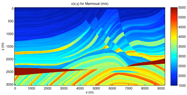
(b)

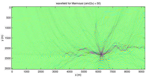
Figure 1: Marmousi model and solution with $\frac{\omega}{2\pi}=50$

$N_{x}\times N_{y}$	$h$ (m)	$\frac{\omega}{2\pi}$ (Hz)	Number of $x$-subdomains
			3	10	30	100	300
$600\times 212$	16	12.5	4	5	6
$1175\times 400$	8	25	5	6	7
$2325\times 775$	4	50	6	6	7	9
$4625\times 1525$	2	100	6	6	7	8
$9225\times 3025$	1	200		7	8	9	13 (8) (*)

(*) $13$ was obtained for $w_{\rm pml}=5$, $8$ for $w_{\rm pml}=6$.

Table 2: Convergence results for example 1. Displayed is the number of iterations for reduction of the residual by $10^{-6}$ as a function of the size of the domain and the number of subdomains.

4.2 Example 2: A random medium in 3-D

Our second example is random medium in 3-D. Plots of the medium and a solution are given in Figure 2. The size of the example varied between $100^{3}$ and $400^{3}$ (excluding PML layers on the sides). In all cases the medium was divided in layers of thickness $10$ (excluding again the PML layers). Experiments were performed with $w_{\rm pml}=4$ and $5$. The thickness of the subdomain on which the computation took place was hence 19 and 21 grid points respectively. The results are summarized in Table 3.

The result are similar to those of the Marmousi examples. The iterative method converged rapidly, in 6 to 8 iterations. In these examples the value $w_{\rm pml}=4$ is sufficient.

(a)

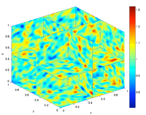
(b)

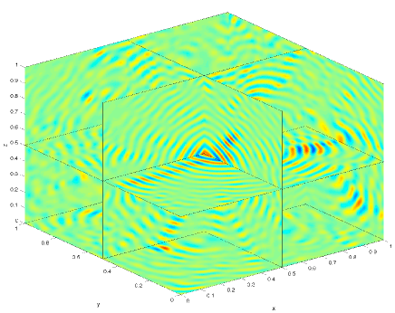
Figure 2: (a) Random medium used in example 2; (b) solution to the Helmholtz equation with a point source.

$n_{x}\times n_{y}\times n_{z}$	$h$	$\frac{\omega}{2\pi}$	$J$	$w_{\rm pml}$
				4	5
$100\times 100\times 100$	0.01	10	10	6	5
$200\times 200\times 200$	0.005	20	20	6	6
$300\times 300\times 300$	0.00333	30	30	7	6
$400\times 400\times 400$	0.0025	40	40	8	6

Table 3: Convergence results for example 2, a random medium in 3-D.

4.3 Example 3: A constant medium in 3-D and varying $w_{\rm pml}$

In our third example we explore the dependence of the convergence on $w_{\rm pml}$. The main conclusion of the previous two examples is that convergence is fast in all cases. Nevertheless, a increase in $w_{\rm pml}$ reduces the number of iterations somewhat in the larger examples.

In this example the domain is the unit cube, and the velocity $c=1$. (A constant medium is attractive because it requires less computational resources, due to the fact that for only one subdomain the $LDL^{t}$ decomposition has to be computed.) The subdomain size varies between $100^{3}$ and $400^{3}$ (excluding the outer PML layers), while the thickness of the PML layers varies between 3 and 6 gridpoints. The frequency $\omega$ is chosen to correspond to 10 grid points per wavelength. The results are given in Table 4.

While we have limited data, still the following pattern can be observed. For fixed $w_{\rm pml}$ the number of iterations increases with the grid size. However the number of iterations can be kept more or less constant if one can increases $w_{\rm pml}$ at the same time as the grid size. Here $w_{\rm pml}$ goes roughly logarithmically with the grid size.

$n_{x}\times n_{y}\times n_{z}$	$h$	$\frac{\omega}{2\pi}$	$J$	$w_{\rm pml}$
				3	4	5	6
$100\times 100\times 100$	0.01	10	10	5	4	4	3
$200\times 200\times 200$	0.005	20	20	7	5	4	4
$400\times 400\times 400$	0.0025	40	40	10	7	5	5

Table 4: Convergence results for example 3. Displayed is the number of iterations for reduction of the residual by $10^{-6}$ as a function of domain size and $w_{\rm pml}$.

4.4 Comparison between Robin and PML-based transmission conditions

Motivated by our results so far, we study a double sweep method with Robin transmission conditions. This appears to be a new combination even though Robin transmission conditions have been extensively studied. We will compare this with the method above.

Similarly as above, we introduce overlapping subintervals of the $x$-axis, here denoted by $]l^{(j)},r^{(j)}[$, $j=1,\ldots,J$, with $r^{(j)}=l^{(j+1)}+m_{\rm overlap}h$, $m_{\rm overlap}$ denoting the overlap in gridpoints (i.e. $l^{(j)}=b_{j}$ and $r^{(j)}=\tilde{b}^{(j+1)}$). In 2-D, for a rectangular domain $]0,L[\times]0,L_{y}[$, the right sweep with Robin transmission conditions amounts to solving the boundary value problems

$$-\partial_{xx}^{2}v^{(j)}-\partial_{yy}^{2}v^{(j)}-k(x)^{2}v^{(j)}={} f^{(j)} l^{(j)}<x<r^{(j)} 0<y<L_{y}$$ for ,

$$\partial_{x}v^{(j)}+ikv^{(j)}={} \partial_{x}v^{(j-1)}+ikv^{(j-1)} x=l^{(j)} 0<y<L_{y}$$ at ,

$$-\partial_{x}v^{(j)}+ikv^{(j)}={} 0 x=r^{(j)} 0<y<L_{y}$$ at ,

for $j=1,\ldots,J$ consecutively, where $f^{(j)}(x,y)=f(x,y)$ for $l^{(j)}<x<l^{(j+1)}$ and zero elsewhere and PML modifications are assumed to be present near all the external boundaries. This results in a an approximate solution given by $v(x)=v^{(j)}(x)$ for $l^{(j)}<x<l^{(j+1)}$. The left sweep uses the residual $g=f-Au$ as right hand side and is otherwise a left-right reflection of the right sweep. This algorithm was implemented in Matlab.

A choice in this algorithm was the overlap parameter $m_{\rm overlap}$. This parameter was set equal to 1, since a zero overlap resulted in significantly worse convergence and larger overlaps did not significantly improve the convergence.

On the unit square tests were performed for a constant medium ($c=1$) and a random medium displayed in Figure 3. We chose $N_{x}$ ranging from 100 to 1600 and $N_{y}=N_{x}$. The layer thickness was set at 10 points. Because of the absence of PML layers, the subdomain solves are roughly 4 times cheaper when using Robin transmission conditions compared to PML based conditions. Iteration numbers for reduction of the residual by $10^{-6}$ are given in Tables 5 and 6.

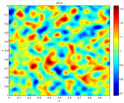
Figure 3: Random medium used for the comparision of Robin and PML-based transmission conditions

$N_{x}\times N_{y}$	$h$	$\frac{\omega}{2\pi}$	$J$	PML	Robin
$100\times 100$	0.01	10	10	3	9
$200\times 200$	0.005	20	20	4	13
$400\times 400$	0.0025	40	40	4	20
$800\times 800$	0.00125	80	80	5	42
$1600\times 1600$	0.000625	160	160	7	103

Table 5: Comparison of convergence between Robin and PML-based transmission conditions for a constant medium.

$N_{x}\times N_{y}$	$h$	$\frac{\omega}{2\pi}$	$J$	PML	Robin
$100\times 100$	0.01	7.14	10	7	11
$200\times 200$	0.005	14.29	20	6	14
$400\times 400$	0.0025	28.57	40	6	20
$800\times 800$	0.00125	57.14	80	7	34
$1600\times 1600$	0.000625	114.3	160	8	74

Table 6: Comparison of convergence between Robin and PML-based transmission conditions for the random medium displayed in Figure 3.

Two conclusions can be drawn. First the method looks very interesting, and certainly seems worthy of further study. On the other hand the remarkable scaling of the PML-based transmission conditions is not reproduced. With the Robin transmission conditions the iteration numbers grow roughly linearly in $N_{x}$, or as $N^{1/2}$ in 2-D. In 3-D this would lead to iteration numbers $O(N^{1/3})$.

We thank one of the anonymous reviewers for suggesting a comparison with Robin transmission conditions.

5 Discussion

A new domain decomposition method for the Helmholtz equation was presented. It has remarkably fast convergence, even in the case of thin-layered subdomains. We have focussed on the use of this method with sparse direct solvers on the subdomains.

The method is related to that of Schädle et al. in [2]. In this reference, the authors consider finite element methods for the time harmonic Maxwell equations on unbounded domains truncated using the perfectly matched layer. A domain decomposition method using PML-based interface conditions is derived using a single sweep in each iteration. While the transmission term is different from the one derived here, the difference is not very relevant since its contribution propagates from the boundary $b_{j}$ directly into the PML layer, not entering the physical domain. Numerical results are given for a 2-D example, using 2 or 3 subdomains, where in the second case the convergence is markedly worse, probably due to the use of a single sweep. We conclude that using a double sweep preconditioner is essential to obtain the good convergence properties.

As pointed out in the introduction, the use of multiplicative domain decomposition implies that the method is by nature sequential. There are basically two ways to obtain good parallel performance. One is the parallellization of the $LDL^{t}$ factorization and backsubstitution steps. Such an approach is described in [25] for the sweeping preconditioner. This is mostly a problem of parallel linear algebra, and not of domain decomposition (although the distribution of the unknowns is relevant for both parts of the story). The second strategy is to divide the subdomains over groups of processing nodes and perform the computation for multiple right hand sides in a pipelined fashion. Because of the setup time, the method is most relevant for the case with multiple right hand sides anyway. (In other cases it probably makes more sense to opt e.g. for the shifted Laplacian method).

The solutions to the time harmonic Maxwell equations and the time harmonic linear elastic wave equation behave in many respects the same as those of the Helmholtz equation. We expect that the techniques outlined in this paper are applicable in those cases as well.

References

References

- Berenger [1994] J.-P. Berenger, A perfectly matched layer for the absorption of electromagnetic waves, Journal of Computational Physics 114 (1994) 185–200.
- Schädle et al. [2007] A. Schädle, L. Zschiedrich, S. Burger, R. Klose, F. Schmidt, Domain decomposition method for Maxwell’s equations: scattering off periodic structures, J. Comput. Phys. 226 (2007) 477–493.
- Engquist and Ying [2011] B. Engquist, L. Ying, Sweeping preconditioner for the Helmholtz equation: moving perfectly matched layers, Multiscale Model. Simul. 9 (2011) 686–710.
- Collino et al. [2000] F. Collino, S. Ghanemi, P. Joly, Domain decomposition method for harmonic wave propagation: a general presentation, Comput. Methods Appl. Mech. Engrg. 184 (2000) 171–211. Vistas in domain decomposition and parallel processing in computational mechanics.
- Després [1991] B. Després, Domain decomposition method and the Helmholtz problem, in: Mathematical and numerical aspects of wave propagation phenomena (Strasbourg, 1991), SIAM, Philadelphia, PA, 1991, pp. 44–52.
- Després [1990] B. Després, Décomposition de domaine et problème de Helmholtz, C. R. Acad. Sci. Paris Sér. I Math. 311 (1990) 313–316.
- Shaidurov and Ogorodnikov [1991] V. V. Shaidurov, E. I. Ogorodnikov, Some numerical method of solving Helmholtz wave equation, in: Mathematical and numerical aspects of wave propagation phenomena (Strasbourg, 1991), SIAM, Philadelphia, PA, 1991, pp. 73–79.
- Benamou and Desprès [1997] J.-D. Benamou, B. Desprès, A domain decomposition method for the Helmholtz equation and related optimal control problems, J. Comput. Phys. 136 (1997) 68–82.
- Gander et al. [2002] M. J. Gander, F. Magoulès, F. Nataf, Optimized Schwarz methods without overlap for the Helmholtz equation, SIAM J. Sci. Comput. 24 (2002) 38–60 (electronic).
- Gander et al. [2007] M. J. Gander, L. Halpern, F. Magoulès, An optimized Schwarz method with two-sided Robin transmission conditions for the Helmholtz equation, Internat. J. Numer. Methods Fluids 55 (2007) 163–175.
- Nataf et al. [1994] F. Nataf, F. Rogier, E. de Sturler, Optimal Interface Conditions for Domain Decomposition Methods, Technical Report 301, Ecole Polytechnique, CMAP, 1994.
- Engquist and Majda [1977] B. Engquist, A. Majda, Absorbing boundary conditions for numerical simulation of waves, Proc. Nat. Acad. Sci. U.S.A. 74 (1977) 1765–1766.
- Chevalier and Nataf [1998] P. Chevalier, F. Nataf, An optimized order 2 (OO2) method for the Helmholtz equation, C. R. Acad. Sci. Paris Sér. I Math. 326 (1998) 769–774.
- Boubendir et al. [2012] Y. Boubendir, X. Antoine, C. Geuzaine, A quasi-optimal non-overlapping domain decomposition algorithm for the helmholtz equation, Journal of Computational Physics 231 (2012) 262 – 280.
- Toselli [1998] A. Toselli, Some results on overlapping Schwarz methods for the Helmholtz equation employing perfectly matched layers, Technical Report 765, New York University, 1998. Cs.nyu.edu/web/Research/TechReports/TR1998-765/TR1998-765.pdf.
- George [1973] A. George, Nested dissection of a regular finite element mesh, SIAM J. Numer. Anal. 10 (1973) 345–363.
- Erlangga [2008] Y. A. Erlangga, Advances in iterative methods and preconditioners for the Helmholtz equation, Arch. Comput. Methods Eng. 15 (2008) 37–66.
- Ernst and Gander [2011] O. G. Ernst, M. J. Gander, Why it is difficult to solve helmholtz problems with classical iterative methods, in: I. Graham, T. Hou, L. O., R. Scheichl (Eds.), Numerical Analysis of Multiscale Problems, Springer, 2011.
- Wang et al. [2011] S. Wang, M. V. De Hoop, J. Xia, On 3d modeling of seismic wave propagation via a structured parallel multifrontal direct helmholtz solver, Geophysical Prospecting 59 (2011) 857–873.
- Bollhöfer et al. [2009] M. Bollhöfer, M. J. Grote, O. Schenk, Algebraic multilevel preconditioner for the Helmholtz equation in heterogeneous media, SIAM J. Sci. Comput. 31 (2009) 3781–3805.
- Chew and Weedon [1994] W. C. Chew, W. H. Weedon, A 3D perfectly matched medium from modified Maxwell’s equations with stretched coordinates, Microwave and Optical Technology Letters 7 (1994) 599–604.
- Johnson [2010] S. G. Johnson, Notes on perfectly matched layers, http://math.mit.edu/ stevenj/18.369/pml.pdf, 2010.
- Amestoy et al. [2001] P. R. Amestoy, I. S. Duff, J.-Y. L’Excellent, J. Koster, A fully asynchronous multifrontal solver using distributed dynamic scheduling, SIAM J. Matrix Anal. Appl. 23 (2001) 15–41 (electronic).
- Davis [2004] T. A. Davis, Algorithm 832: UMFPACK V4.3—an unsymmetric-pattern multifrontal method, ACM Trans. Math. Software 30 (2004) 196–199.
- Poulson et al. [2012] J. Poulson, B. Engquist, S. Fomel, S. Li, L. Ying, A parallel sweeping preconditioner for high-frequency heterogeneous 3D Helmholtz equations, Technical Report, University of Texas at Austin, 2012. Http://www.math.utexas.edu/users/lexing/publications/parallelsweeping.pdf.