Trace transform based method
for color image domain identification

Abstract

Context categorization is a fundamental pre-requisite for multi-domain multimedia content analysis applications . Most feature extraction methods require prior knowledge to decide if they are suitable for a specific domain and to optimize their input parameters. In this paper, we introduce a new color image context categorization method (DITEC) based on the trace transform. We also analyze the distortions produce by the parameters that determine the sampling of the discrete trace transform. The problem of dimensionality reduction of the obtained trace transform signal is addressed through statistical descriptors that keep the underlying information. Moreover, Feature Subset Selection (FSS) is applied to both, improve the classification performance and compact the final length of the descriptor. These extracted features offer a highly discriminant behavior for content categorization. The theoretical properties of the method are analyzed and experimentally validated through two different datasets.

1 Introduction

The importance of semantic context is very well known in Content Based Image Retrieval (CBIR) [1, 2]. This is especially relevant for broad-domain data intensive multimedia retrieval activities such as TV production and marketing or large-scale earth observation archive navigation and exploitation. Most modeling approaches rely on local low-level features, based on shape, texture, color etc. The drawback of these methods is that the characterization of the context requires prior contextual information, introducing a chicken-and-egg problem[3]. A possible approach to try and reduce this dependency involves the exploitation of global image context characterization for semantic domain inference. This prior information on scene context could represent a valuable asset in computer vision for purposes ranging from regularization to the pre-selection of local primitive feature extractors [4].

Novel semantic approaches that try to overcome the current existing limitation derived from fixed taxonomies and manual annotations, rely on automatic or semi-automatic ingestion processes. These processes minimize the semantic gap by introducing semantic middleware [5] layers based on a combination of:

• explicit information provided by human made taxonomies.

• relevance feedback data and knowledge extracted from manual annotations.

• implicit information obtained by data mining techniques through training processes.

The major contributions made in this paper are:

• A new methodology for global feature extraction based on a statistical modeling of the trace transform in the frequency domain.

• An analysis of the effects of the discrete trace transform in order to establish the best sampling parameters.

• An analysis of the resulting feature space to have an estimation of the results that can be obtained with machine learning techniques

• A demonstration that DITEC provides highly discriminative global descriptors at very low dimensionality, a key factor for efficient retrieval in massive content databases [6][7].

• DITEC is very suitable for domain classification, especially for those cases where the lack of prior knowledge does not allow the effective use of specific local features.

1.1 Related works

Research contributions related to the approach proposed in this paper are outlined in this section.

Local features have been used broadly for context categorization [8, 9]. SIFT[10] and SURF[11] are among most popular choices in this respect. A two step approach for the efficient use of local features has been proposed by several authors such as Ravinovich et al. [12] and Choi et al.[13]. Olaizola et al. [14] have proposed an architecture for hypothesis reinforcement based on an initial analysis of low-level features for context categorization and further hypothesis creation. This architecture can exploit context specific feature extractors to validate or refuse the initial context hypothesis. This stresses the value of global descriptors for initial domain categorization purposes. Once a specific domain has been identified, different low-level features can be extracted. However, these features cannot be combined in a simple way and the obtained multi-attribute spaces must be normalized in order to be used in similarity search or retrieval tasks [15].

Among different global descriptors such as histograms of several local features [16], texture features, self similarity [17], there are some specific algorithms in the literature which have shown great potential: GIST[18, 19] is probably one of the most popular ones. Watanabe et al. [20] have proposed a global descriptor based on the codewords provided by Lempel-Ziv entropy coders [21, 22], exploiting the relationship between the complexity of an image and the context in which it may belong. The Ridgelet transform [23, 24, 25] has been successfully used as a global feature for image categorization and handwritten character recognition. In typical operational implementations, all these algorithms are typically combined with other global or local features.

The trace transform has already been proposed for several computer vision applications. Indeed, a method based on this transform has been included in the MPEG-7[26] standard specification for image fingerprinting[27, 28]. Other applications (mostly with monochrome images) include face recognition[29, 30, 31, 32], character recognition[33] and sign recognition[34]. The proposed approach based on a recursive application of the trace transform to reduce the dimensionality of the obtained feature space (known as the triple feature), offers an excellent performance for image fingerprinting, but does not offer good discriminative characteristics as a method for domain characterization due to the high data loss incurred by the diametrical and circus functionals [35].

The approach proposed by Liu and Wang [31] reduces the number of attributes using Principal Component Analysis (PCA) to select the most relevant coefficient and reduce the dimensionality of the feature space. However, this approach does not take into account the frequency relationships among the different coefficients and increases the feature extraction complexity as it requires the covariance matrix information of all previous samples. Moreover, the feature relevance of each individual DCT coefficient is too low and also sensitive to noise and variations.

Li et al. [36] have proposed a generalization of the Radon transform and trace transform by introducing prior knowledge of specific identification or fingerprinting tasks and extending the geometric sets from straight lines to arbitrary choices. This approach provides a complete set of resources for non-rigid object identification and has been successfully tested for pedestrian recognition, part segmentation and video retrieval. However, the broad set of configuration parameters and pre-processing tasks are not suitable for domain identification purposes where the lack of a priori knowledges is one of the main issues.

This paper is organized as follows: In Section 2 a general overview of our proposed DITEC method is presented. In Section 2.1, image pre-processing issues are addressed. The trace transform and its properties are analyzed in Section 2.2. Feature extraction process details are presented in Section 2.3 while the classification process is described in Section 2.4. The validation carried out with two different datasets is explained in Section 3. The computational complexity of the DITEC framework is analyzed in Section 4. Finally, Section 5 concludes with a discussion of the results.

2 General Description of the DITEC method

The DITEC method is composed of four main steps where an observed image $D$ is estimated as $\hat{C}$ of the unknown global image semantic concept $C$ (Figure 1).

Figure 1: DITEC System workflow

The four DITEC steps are thus the following:

• Sensor modeling: image acquisition and pre-processing (radiometric noise, color space, geometric quantization and image lattice finiteness effects).

• Data transformation: trace transform (detailed in 2.2) applied to the pre-processed image $I$. The result will depend on the chosen functional (e.g: (18)) and on the selected geometric parameters (detailed in Section 2.2.3). The outcome $T$ of the trace transform of an image is a two-dimensional signal represented by means of sinusoids with a particular amplitude, phase, frequency and intensity. This characterization process represents one of the key steps in the overall information extraction process.

• Feature extraction: summarization of the extracted features $T$, compressed and adapted into a manageable set $E$ of object-based descriptors. The wave features contained in the resulting image must be characterized. In order to do this,the 2D trace signal $T_{k}$ is transformed to the frequency domain. To concentrate the signal energy to the lowest spatial frequencies, a two-dimensional DCT (Discrete Cosine Transform) is applied. Then, the DCT is compressed to a vector of two components (average value and kurtosis of all the orthogonal elements of the main diagonal, Figure 6). This transformation considers the DCT space as representable by a superposition of leptokurtic distributions. It aims to reduce the considered descriptor space dimensionality while preserving essential information in order to allow a good performance in the subsequent classification process. The last $n$ values from the obtained data pair vector can be disregarded due to the empirical reason that given the low-pass filtering for most natural images the DCT concentrates the highest values in the lowest coefficients.

• Class assignment: vectors obtained in the previous step are processed to improve the performance of classifiers in the defined feature space. All the obtained vectors are statistically analyzed to select their most representative attributes. Then the supervised classification process is carried out to obtain an estimate $\hat{C}$ of the unknown global image semantic concept $C$.

2.1 Sensor modeling

The first pre-processing step transforms the $RGB$ color space into $YC_{b}C_{r}$[37]. The luminance channel ($Y$) will be used as the most relevant channel to encode shape related features. Color distribution information is encoded by processing the chrominance channels ($C_{b},C_{r}$).

In order to reduce effects introduced by radiometric noise, image lattice and quantization, a low-pass filter is applied to each channel.

HSV [37] color space information is encoded by obtaining mean and variance values ($\mu,\sigma$) of the corresponding intensity distributions in each H,S,V channel. In the Attribute Selection process, this ($\mu,\sigma$) information is introduced into the obtained descriptor $E$.

2.2 Data transformation

The data transformation process is carried out through the trace transform, a generalization of the Radon transform (1) where the integral of the function is substituted for any other functional $\Xi$ [38, 35, 39, 34, 40].

$$R(\phi,\rho)=\iint f(x,y)\delta(x\cos{\phi}+y\sin{\phi}-\rho)dx\;dy$$ (1)

The trace transform consists of applying a functional $\Xi$ along a straight line (L in Figure 2). This line is moved tangentially to a circle of radius $\rho$ covering the set of all tangential lines defined by $\phi$. The Radon transform has been used to characterize images [41] in well defined domains [42], in image fingerprinting [43] and as a primitive feature for general image description. The trace transform extends the Radon transform by enabling the definition of the functional and thus enhancing the control on the feature space. These features can be set up to show scale, rotation/affine transformation invariance or high discriminance for specific content domains.

Figure 2: Trace transform, geometrical representation

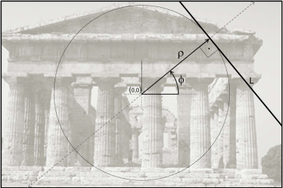
The outcome $T$ of the trace transform of a 2D image is another 2D signal composed by a set of sinusoidal shapes that vary in amplitude, phase, frequency, intensity and thickness. These sinusoidal signals encode the pre-processed image $I$ with a given level of distortion depending on the functional and quantization parameters.

2.2.1 Functionals

A functional $\Xi$ of a function $\xi(x)$ evaluated along the line $L$ will have different properties depending on the features of function $\xi(x)$ (e.g.: invariance to rotation, translation and scaling[44]). Kadirov et al. [45] propose several functionals with different invariance or sensitiveness properties. These invariant functionals have been used for expert systems for traffic sign recognition [34], face authentication[30, 46] or fingerprinting [35] purposes.

2.2.2 Geometrical constraints

The result of the discrete trace transform strongly depends on the selected geometrical parameters. The three resolution parameters denoted by $\Delta\phi,\Delta\rho,\xi(\Delta L)$ respectively for angle, radius and the sampling rate along the line $L$, establish distortions and aliasing effects that will affect the final result of the trace transform.

The final resolution of the sinogram $T$ obtained by applying the trace transform will be defined by $n_{\phi}$ and $n_{\rho}$ where:

$$n_{\phi}=\frac{2\pi}{\Delta\phi}$$ (2)

$$n_{\rho}=\frac{\min(X,Y)}{\Delta\rho}$$ (3)

with $X$ and $Y$ denoting the horizontal and vertical resolutions of the image $I_{l}$.

Low $(n_{\phi},n_{\rho},n_{\xi})$ values will have a non-linear downsampling effect on the original image, where $n_{\xi}$ is defined as:

$$n_{\xi}=\frac{1}{\Delta L}$$ (4)

The set of points used to evaluate each functional is described (assuming (0,0) as the center of the image) by:

$$y=2\rho\sin(\phi)-\frac{x}{\tan(\phi)}$$ (5)

A singularity can be observed at $\phi=0$ and $\phi=\pi$. For these cases it can be assumed that:

$$\begin{array}[]{rllll}x=&\rho&\forall y&if&\phi=0\\ x=&-\rho&\forall y&if&\phi=\pi\\ \end{array}$$ (8)

The range of the parameters is :

$$\phi\in[0,2\pi]$$ (9)

$$\rho\in\left[-r,r\right],r=\min\left(\frac{\frac{X}{2}}{\cos(\phi)},\frac{\frac{Y}{2}}{\sin(\phi)}\right)$$ (10)

$$\begin{array}[]{l}x\in\left\{\begin{array}[]{rcl}\left[-\frac{\textstyle X}{\textstyle 2},\frac{\textstyle X}{\textstyle 2}\right]&\forall&\phi\in\alpha\\[15.0pt] \left[-\frac{\frac{\textstyle Y}{\textstyle 2}}{\textstyle\tan(\phi)},\frac{\frac{\textstyle Y}{\textstyle 2}}{\textstyle\tan(\phi)}\right]&\forall&\phi\in\beta\end{array}\right\}\\[40.0pt] \textstyle\alpha\in\left[-\frac{\textstyle\pi}{\textstyle 4},\frac{\textstyle\pi}{\textstyle 4}\right]\cup\left[\textstyle-\frac{\textstyle 3\pi}{\textstyle 4},\frac{\textstyle 5\pi}{\textstyle 4}\right]\\[15.0pt] \textstyle\beta\in\left(\frac{\textstyle\pi}{\textstyle 4},\frac{\textstyle 3\pi}{\textstyle 4}\right)\cup\left(\frac{\textstyle 5\pi}{\textstyle 4}\frac{\textstyle 7\pi}{\textstyle 4}\right)\end{array}$$ (11)

$X$ and $Y$ are the horizontal and vertical resolutions of the image. Equation (5) shows a symmetrical result since the same lines are obtained for $\phi\in[0,\pi]$ and $\phi\in[\pi,2\pi]$. However this is only true for functionals that are not considering the position (like the Radon transform). Depending on the selected functional and on the desired properties of the trace transform(e.g: rotational invariance), the ranges of $\phi$ and $\rho$ can be modified to: $\phi\in[0,\pi]$ or $\rho\in[0,r]$.

2.2.3 Quantization effects

Digital images are affected by two main effects during trace transformation:

Figure 3: Trace transform contribution mask at very high resolution parameters (Image resolution:100x100px. $n_{\phi}=1000,n\rho=1000,n_{\xi}=5000$).

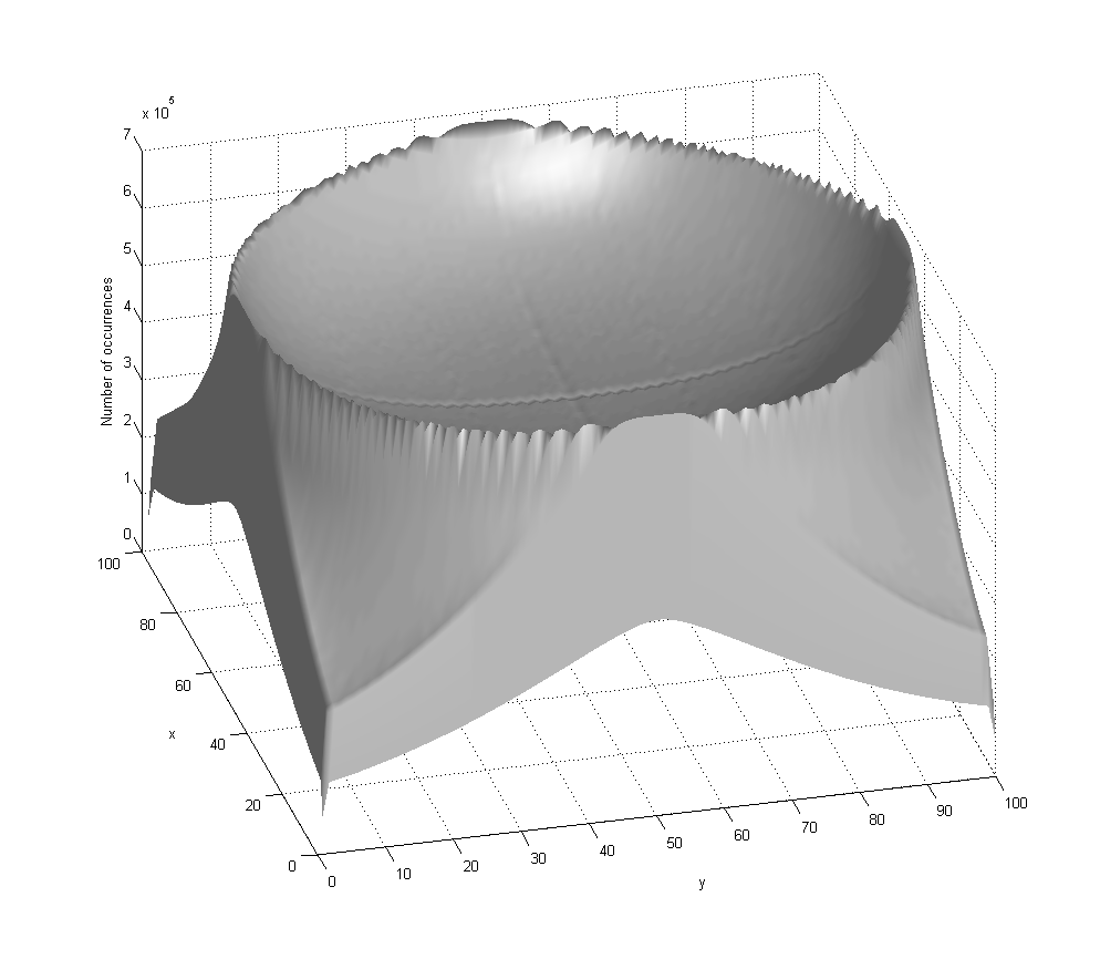
• some pixels might never be used by the functional given the geometrical setup of the transform, and to its integration nature.

• there may be some pixels that have much higher cumulated effect than the others into the functional.

In this section we will analyze the effects that need to be taken into account in order to preserve the homogeneity of the results, avoiding pixels or areas with higher relevance than others. Even for very high ($n_{\phi},n_{\rho},n_{\xi}$) values in relation to the original image resolution, the trace transform introduces a contribution intensity map that encodes the relevance of the different regions of the input picture. As shown in Figure 3, high resolution values of the trace transform parameters tend to create a convex contribution intensity map. Therefore, high parameter values do not necessarily imply optimal image content representation on the trace transform.

High values of $n_{\phi}$ improve the rotational invariance of the trace transform (although in such a manner that it is dependent on the selected functional) while very low values $n_{\phi}<5$ cannot be considered as producing a valid trace transform since there is not enough angular information.

(a) Original

(b) (64,64,15)

(c) (64,64,45)

(d) (64,64,185)

(e) (5,300,45)

(f) (5,300,151)

(g) (300,5,45)

(h) (300,5,151)

Figure 4: Pixels relevance in trace transform scanning process with different parameters $(n_{\phi},n_{\rho},n_{\xi})$. Original image resolution = 384x256.

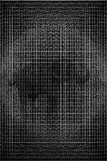
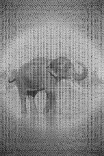
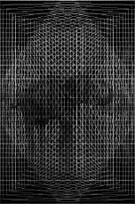
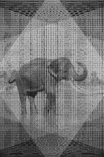
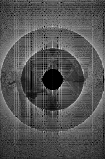
Ideally, the trace transform should keep the following constraints (considering $M$ as the matrix that contains the number of repetitions of each pixel during the trace transform):

• Coverage: all pixels of the image (including those located at the corners of the image) have to be included in at least one functional. $\min(M)>0$.

• Homogeneity: all pixels are used the same number of times. $\text{Var}(M)=0$ .

• High pixel repetition degree: each pixel has to be included in as many traces as possible (high values of $mean(M))$.

TABLE I: Quantization effects of the trace transform

			% pixels
$\boldsymbol{n_{\phi}}$	$\boldsymbol{n_{\rho}}$	$\boldsymbol{n_{\xi(L)}}$	used	Mean	Var
64	64	15	16.60	0.63	15.71
64	64	45	44.30	1.88	32.72
64	64	85	67.53	3.54	53.61
64	64	185	93.40	7.71	52.51
300	5	45	28.62	0.69	10.28
300	5	151	69.84	2.30	31.80
5	300	45	40.59	0.68	0.20
5	300	151	88.43	2.30	0.42
5	300	218	97.34	3.33	0.40
5	300	251	99.18	3.83	0.30
384	256	15	83.76	15.00	1.2$\cdot$106
100	100	85	85.55	8.65	872.47
100	100	185	98.72	18.82	708.64
100	100	218	99.55	22.18	511.61
100	100	2,185	100.00	222.27	3.6$\cdot$106
42	75	12,000	99.77	384.52	38.6$\cdot$106

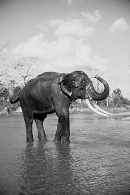
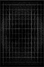
Table 2.2.3 shows some example values for coverage, homogeneity and repetition degree at different $n_{\phi},n_{\rho},n_{\xi}$ resolutions. Note that the best ratios are obtained for lower variations in $\phi$ as the angle is the main factor to increase the variance. The pixel repetition degree is also strongly conditioned by the angular resolution. This fact makes $n_{\phi}$ the main factor to balance the homogeneity and repetition degree (e.g: low repetition degrees show weaker rotational invariance). Once $n_{\phi}$ is set, $n_{\rho}$ can be adjusted to ensure the optimal coverage. $n_{\xi}$ has an almost asymptotic behavior once the other two parameters are set and can be optimized ensuring a minimum pixelwise sampling. However, these different sampling techniques (e.g.: fixed sampling step or Bresenham algorithm[47]) can also introduce some distortions produced by the different number of samples for each ($\rho,\phi$) combination. Figure 4 shows some cases applied to a real image and the convex contribution intensity mask effect for different values of $n_{\phi}$.

2.3 Feature extraction

Diametric and Circus transform have been used mostly in the literature [39, 45, 40, 27] to reduce the set of descriptors . However, even if this approach provides good results for similarity search or image hashing, the diametric and circus transform do not preserve the information. In fact, there is no inverse transform for these two operators.

In order to characterize the sinograms obtained from the trace transform ($T$), we propose the frequency analysis of the obtained signal and a representation based on statistical descriptor of the frequency distribution. To do this, DFT Discrete Fourier Transform (DFT) or Discrete Cosine Transform (DCT) can be applied. The DCT [48], which has become one of the most popular transforms for audio and image coding, has two main properties which make it more suitable than DFT for the feature extraction process: energy compaction and decorrelation [49]. The energy compaction means that the signal energy is accumulated in a small number of coefficients and that these coefficients are typically the lowest coefficients of the DCT transform. Taking into account that the trace transform does not introduce high frequencies into the transformed image, the DCT provides a good method to efficiently represent the wave-like signal information contained in the resulting images. The decorrelation property of the DCT implies that there is a very low interdependency among the coefficients. This property matches with the common needs of a number of data mining algorithms whose performance has a strong dependency on input attribute correlation. Moreover, the coefficients obtained by applying a DCT are real values while the DFT provides coefficients in the complex domain. The DCT thus allows us to encode information in lower dimensionality code spaces with better compaction characteristics. Moreover, from the computational cost point of view, there are efficient DCT implementations that make it suitable for real-time applications without high computing performance requirements.

The 2D forward DCT is given by:

$${\displaystyle\begin{array}[]{c}\displaystyle X_{k_{1}k_{2}}=\displaystyle\alpha_{k_{1}}\alpha_{k_{2}}\sum^{N_{1}-1}_{n_{1}=0}\displaystyle\sum^{N_{2}-1}_{n_{2}=0}x_{n_{1}n_{2}}\cos\left[\frac{\pi k_{1}(2n_{1}+1)}{2N_{1}}\right]\cdot\\[20.0pt] \displaystyle\cos\left[\frac{\pi k_{2}(2n_{2}+1)}{2N_{2}}\right]\end{array}}$$ (14)

where:

$$\alpha\in\left\{{\scriptstyle\begin{array}[]{rl}\displaystyle\frac{1}{\sqrt{N_{i}}}&k_{i}=0\\[15.0pt] \displaystyle\sqrt{\frac{2}{N_{i}}}&k_{i}\neq 0\end{array}}\right.$$ (17)

2.3.1 Statistical descriptors

As a consequence of the properties of the DCT and of the nature of the 2D signals resulting from the trace transform, the 2D DCT stores more energy in its lower frequencies.

(a) Original

(b) Trace transform (F3)

(c) DCT2 4 level quantization

Figure 5: Trace Transform and subsequent Discrete Cosine Transform of Lenna. (Y channel of YCbCr color space)

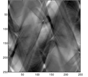
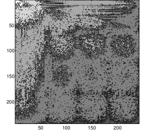
Figure 5 shows the process of trace transform evaluation and its 2D DCT where the intensity is quantized into 6 different levels. The functional used is the one enumerated by Kadyrov et al. [35] as invariant functional IF2 (18).

$$T_{IF2}=\left(\int\left|\xi(t)\right|^{q}dt\right)^{r}$$ (18)

This functional has invariance properties for independent variable and function scaling (21):

$$\begin{array}[]{lr}\displaystyle\Xi(\xi(ax)=\alpha(a)\Xi(\xi(x))&\forall{a}>0\\ \displaystyle\Xi(c\xi(x)=\gamma(c)\Xi(\xi(x))&\forall{c}>0\\ \end{array}$$ (21)

where:

$$\begin{array}[]{rrr}\displaystyle\alpha(a)=a^{\kappa_{\Xi}}&\text{and}&\gamma(c)=c^{\lambda_{\Xi}}\\[15.0pt] \end{array}$$ (23)

In the particular case of the IF2 functional, the invariance relation is given by: $\kappa=-r$ and $\gamma=qr$. Experimental tests demonstrate that the best performance is obtained by $r=0.5$ and $r=2$. These values match those proposed by Kadirov et al. [45].

In order to reduce the dimensionality of the obtained coefficients the $n$ first orthogonal straight lines to the main diagonal of the transformed signal $T$ are statistically characterized (Figure 6). These coefficients which correspond to similar frequency bands can be computed very efficiently and provide a high dimensionality reduction ratio.

Figure 6: Conceptual scheme: DCT matrix transformation into ${\mu,k}$ pair vector.

To study these statistical properties, over 50000 sample vectors have been analyzed using the 1000 sample images of Corel 1000 dataset (described in section 3.1). The analysis of obtained histograms shows strong leptokurtic distributions for all samples. Equation (24) defines the kurtosis of a distribution which is represented by (25) for a discrete set of elements. A distribution is considered leptokurtic when $k>3$. For all analyzed distributions the minimum kurtosis value has been greater than 30. More detailed statistical properties are shown in Figure 7.

$$k=\frac{E(x-\mu)^{4}}{\sigma^{4}}$$ (24)

$$k=\frac{\frac{1}{n}\sum\limits_{i=1}^{n}{(x_{i}-\bar{x})^{4}}}{\left(\frac{1}{n}\sum\limits_{i=1}^{n}{(x_{i}-\bar{x})^{2}}\right)^{2}}$$ (25)

Figure 7: Statistical properties of all Kurtosis measurements made on the distributions obtained by processing Corel 1000 dataset

Assuming the leptokurtic nature of the obtained distributions, the list of values can be represented by the mean value and the kurtosis of each vector. This pair of descriptors ($\mu,k$) of the first element (corresponding to the DC value of the DCT) is substituted by the mean and variance of the original image in HSV space. Considering that the mean and kurtosis values encode the information of coefficients corresponding to approximately similar frequencies. The obtained dimensionality of the transformed $(\mu,k)$ pairs is given by (26).

$$nDims=\sqrt{n_{\phi}^{2}+n_{\rho}^{2}}\cdot n_{c}\cdot n_{f}$$ (26)

where $n_{c}$ is the number of channels of the original image and $n_{f}$ the number of features extracted from each vector (2 in the case of using $[\mu,k]$). Thus, the dimensionality reduction is given by (27).

$$r_{f}=\frac{{n_{\phi}}{n_{\rho}}}{\sqrt{n_{\phi}^{2}+n_{\rho}^{2}}\cdot n_{f}}$$ (27)

For square resolutions and considering $n_{f}=2$ the reduction factor increases linearly with the resolution (28).

$$r_{f}=\frac{n^{2}}{n\cdot n_{f}\sqrt{2}}=\frac{n}{2\sqrt{2}}$$ (28)

2.4 Classification

After the feature extraction process explained in the previous section, a set of features $E$ is obtained. The dimensionality of $E$ can be reduced by attribute selection strategies in order to improve the efficiency of subsequent classification steps.

2.4.1 Feature Subset Selection in Machine Learning

Considering machine learning as a set of techniques to discover and extract knowledge in an automated way [50], the basic problem is concerned with the induction of a model which classifies a given object into one of several known classes. In order to induce the classification model, each element $E$ described by a pattern of $d$ features is simplified by applying the Feature Subset Selection (FSS) [51] approach. FSS can be reformulated as follows: given a set of candidate features, select the “best” subset in a classification problem. In our case, the “best” subset will be the one with the best predictive accuracy.

Most of the supervised learning algorithms perform rather poorly when faced with many irrelevant or redundant (depending on the specific characteristics of the classifier) features. In this way, the FSS proposes additional methods to reduce the number of features so as to improve the performance of the supervised classification algorithm.

There are two main approaches to tackle the Feature Subset Selection (FSS) problem from the Machine Learning point of view [52], namely wrapper and filter methods.

Wrapper approaches [53] try to identify the subset of variables that, given a classification paradigm and a dataset, provide the best classification function. The process consists on searching an optimal feature sub-space based on a performance measure (typically the accuracy, though other measures can be used). Each subset is evaluated by testing the performance of the chosen paradigm in the dataset, using only the variables in the subset for evaluation. The estimation of the performance of the classifiers requires a validation scheme, such as cross validation or bootstrap estimation. As a result, the evaluation of each subset involves the training and testing of several classification functions, increasing the computational time required for the FSS process.

The filter approaches search for the best variable subset, independently of the classification paradigm, considering the relationship between the predicting variables and the class, and occasionally the relationship between the predicting variables. One of the simplest approaches consists of ranking the variables according to their usefulness and selecting only those at the top of the ranking. The usefulness of a variable is measured univariately by means of different metrics.

Once the features are ranked, a threshold must be set to obtain the final subset. The ranking methods are only concerned with the relevance of the features considered and, thus, they do not filter out redundant variables.

The selected classifiers are briefly described below; a wrapper Feature Subset Selection has been used in this paper.

For the supervised learning task, in the training set used to generate the classification model, for each $x$ sample its $y$ label value is known. For this analysis, Bayesian Networks [54] and Support Vector Machines (SVM) [55] have been used.

2.4.2 Attribute contribution analysis

In order to appreciate the attribute contributions to the classification task, different approaches can be taken; on the one hand, used attributes could be considered as specifically constructed to the classification problem at hand, and therefore perform a study similar to that of Kumar et al. [56]. On the other hand, the individual contribution of each attribute could be analyzed, using the same classifier and looking at the accuracies obtained [57].

The study of Kumar et al. [56] is based on the analysis of the behavior of binary classifiers, and therefore can hardly be adapted to multi-class problems, although it is possible to perform a similar one based on a pair-wise division of the classification task [58]. Nevertheless, such a deep analysis of the attribute contribution could digress the goal of this paper, and therefore we have decided to perform an analysis of the contribution of the attributes from the classification accuracy point of view.

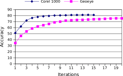
In order to do that, first the accuracy of each of the individual attributes has been computed. Following, a greedy experiment has been performed in order to select the best attribute in each step, and continue selecting features until no improvements have been reached. Figure 8 shows the evolution of the obtained accuracies for each step. As can be seen the evolution of the accuracy is similar in both case studies: the best feature obtains an accuracy of about 35% in the Corel-1000 dataset and of about 50% in Geoeye, but the evolution increases these accuracies to about 80% in both cases.

Figure 8: Accuracy during the FSS process

3 Experimental Results

The presented method has been tested with 2 different datasets. The first of them (Corel 1000 [59]) is a standard dataset which will allow the comparison of the obtained validation data with other methods existing in the literature. The second case (earth observation data), will be used to show the potential of the proposed method under diverse conditions. For both cases, the obtained feature space will be analyzed by establishing metrics that will help to predict the behavior of applied machine learning techniques. A 10-fold cross validation has been used in both cases to split the data into training and testing sets.

3.1 Case study 1: Corel 1000 dataset

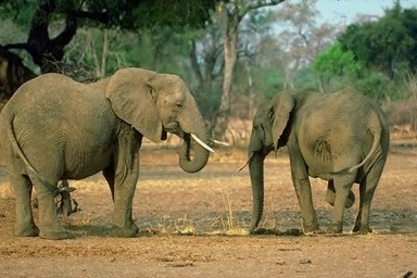
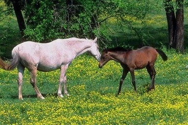
The Corel 1000 dataset is composed of 1000 images distributed in 10 classes (100 instances per class). The tags of the classes are: Africans, Beach, Architecture, Buses, Dinosaurs, Elephants, Flowers, Horses, Mountains and Food. Figure 2.2.3 shows one sample per each class. Even though they are semantically separated, visual similarities may be found among some of them. For example, people and trees can be found under Africa, Beach, and Mountain categories.

(f) Elephants

(g) Flowers

(h) Horses

(i) Mountains

(j) Food

Figure 9: Samples of Corel 1000 dataset. The dataset includes 256x384 or 384x256 images.

The following parameters have been selected: $n_{\phi}=71,n_{\rho}=71,n_{c}=3,n_{f}=2$. This choice results in 15,123 trace transform coefficients per image. By obtaining the mean values and kurtosis as described in the previous section, the number of attributes is reduced to 606 (by a factor of 25).

Based on the fact that the DCT gathers signal energy in the lower frequencies (see Figure 4c), highest coefficients are removed. Moreover, it can be assumed that chrominance channels ($C_{b}$ and $C_{r}$) contain less visual information and therefore more coefficients can be removed from these channels than from the luminance signal ($Y$). Experimental results carried out with different combination of $YC_{b}C_{r}$ coefficients, demonstrate that luminance related attributes have more relevance than chrominance related ones. The selected parameters for this example result in 202 attributes per channel. We will select the first 104 ones for $Y$ and 60 for each $C_{b}C_{r}$ signal, thus reducing the total amount of attributes to 224.

TABLE II: Corel 1000 dataset confusion matrix. Ground truth represented in rows, predicted labels in columns. Labels correspond to the assignment in Figure 2.2.3. F–Measure is the harmonic mean: $F=2\cdot\frac{precision\cdot recall}{precision+recall}$.

	a	b	c	d	e	f	g	h	i	j	Precision	Recall	F–Measure
a	75	2	6	0	2	5	0	2	1	7	0.75	0.75	0.75
b	5	79	6	1	0	6	0	0	2	1	0.752	0.79	0.771
c	3	4	78	1	0	3	1	0	8	2	0.772	0.78	0.776
d	3	3	3	81	0	0	1	0	4	5	0.9	0.81	0.853
e	0	0	0	0	100	0	0	0	0	0	0.98	1	0.99
f	7	1	3	0	0	83	0	2	3	1	0.806	0.83	0.818
g	1	1	0	0	0	0	95	2	0	1	0.941	0.95	0.945
b	1	0	1	1	0	0	0	97	0	0	0.942	0.97	0.956
i	0	14	4	1	0	3	0	0	78	0	0.813	0.78	0.796
j	5	1	0	5	0	3	4	0	0	82	0.828	0.82	0.824
Average											0.848	0.848	0.848

The best performance has been obtained by applying a SVM classifier (accuracy = 84.8% in a k-fold 10 test). 117 attributes have been selected for the final feature space by applying FSS. The information provided by the confusion matrix (Table II) can be represented graphically in order to represent the qualitative behavior of the method. We have selected the Force Atlas 2 algorithm [60] to distribute the classes on a 2D plane. Force Atlas 2 establishes a force directed layout simulating a physical system where nodes (classes) repulse each other and edges apply an attraction force. For the method presented in this paper, the repulsion force is adjusted to scale the layout to a convenient size while edge forces are represented by the error information stored in the confusion matrix. Thus, the attraction force of two nodes will be proportional to the mutual miss-classifications.

For the Corel 1000 dataset, it can be observed in Figure 10 that Dinosaurs, Flowers and Horses are clearly separated from the rest of the categories. This result can also be verified via the precision and recall data. Precision is above 94% and there are very few instances for other classes estimated as Dinosaurs, Flowers or Horses.

Figure 10: Distance among classes in the Corel 1000 dataset according to misclassified instances.

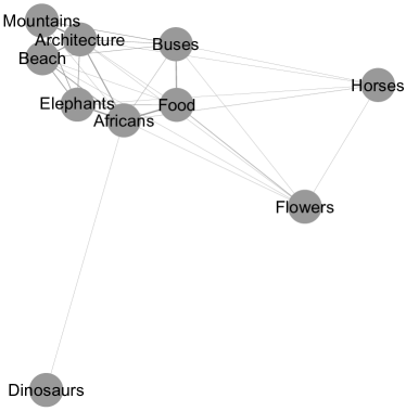
A deeper analysis of class distribution can be performed by removing the aforementioned three categories. Figure 11 shows that there is a group formed by Beach, Mountains and Architecture and other by Africans which links to Elephants and Food although these two are not directly connected.

Figure 11: Distance among most inter-related classes in the Corel 1000 dataset according to misclassified instances.

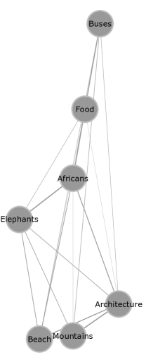
Figure 12 shows an example of one of the classification errors. As it can be seen, the presence of vegetation and trees associates the image to the Mountain class even if it belongs to Architecture. These semantic overlays of Corel 1000 categories put some visually similar images in different classes.

Figure 12: Corel 1000 picture corresponding to class Architecture and classified as Mountain

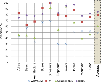
Comparing the obtained results with other feature extraction approaches (Mean-Shift and Gaussian Mixtures based on Weighted Color Histograms[16], Reduced Feature Vector with Relevance Feedback[61] and SIFT based Gaussian Naïve Bayesian Network [62]), DITEC shows the best performance for most categories (Figure 13) and the highest mean precision value. Other performance parameters (such as recall, F–Measure) have not been compared since they have not be indicated in the papers related with the rest of the methods.

Figure 13: Corel 1000 precision results with different feature extraction algorithms. WHMSGM: Mean-Shift and Gaussian Mixtures based on Weighted Color Histograms, FVR: Reduced Feature Vector with Relevance Feedback, Gaussian NBN: SIFT based Gaussian Naïve Bayesian Network.

3.2 Case study 2: Geoeye satellite imagery

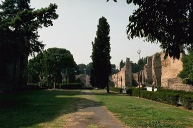
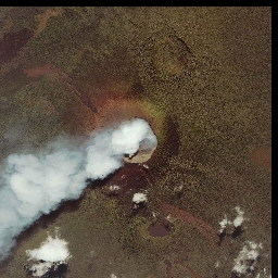
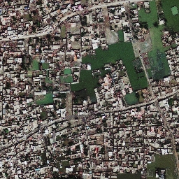
The Geoeye [63] dataset is composed by 1003 multi-resolution patches of Digital Globe Earth observation satellite imagery with up to $\sim 1$m spatial resolution. The dataset is categorized in 7 classes corresponding to different geographical locations (Figure 2.2.3). All the resolutions have been processed with the same trace transform parameters.

(e) Nyragongo

(f) Risalpur

(g) Rome

Figure 14: Samples of satellite footage dataset. 256x256px patches at different scales.

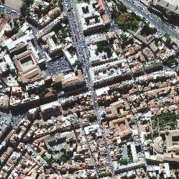
During the data mining process Bayesian networks have shown the best performance, reaching an accuracy of 94.51% in a k-fold 10 test. The final dimensionality of the feature space has been reduced to 61 attributes. Table III shows the confusion matrix of the classification results.

TABLE III: Geoeye dataset confusion matrix. Ground truth represented in rows, predicted labels in columns. Labels correspond to the assignment in Figure 2.2.3. F–Measure is the harmonic mean: $F=2\cdot\frac{precision\cdot recall}{precision+recall}$.

	a	b	c	d	e	f	g	Precision	Recall	F–Measure
(a) Athens	74	0	1	0	2	0	0	0.961	0.961	0.961
(b) Davis	0	183	0	0	2	7	2	1	0.943	0.971
(c) Manama	1	0	193	0	0	0	0	0.97	0.995	0.982
(d) Midway	2	0	0	62	1	0	0	1	0.954	0.976
(e) Nyragongo	0	0	4	0	77	2	2	0.939	0.906	0.922
(f) Risalpur	0	0	0	0	0	177	17	0.898	0.912	0.905
(g) Rome	0	0	1	0	0	11	182	0.897	0.938	0.917
Average								0.946	0.845	0.945

Figure 15: Distance among classes in the Geoeye dataset according to misclassified instances.

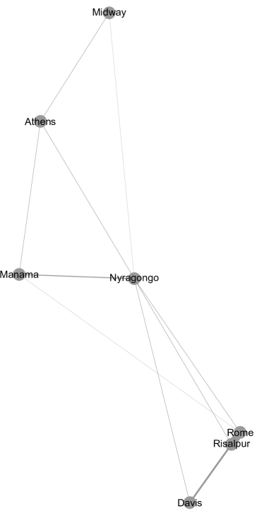
Applying the Force Atlas 2 method to Geoeye classification errors, we obtain the distribution shown in Figure 15. It can be observed that Risalpur and Rome are the categories with the highest mutual similarity (2 cities). The Davis-Monthan aircraft boneyard has shown a remarkable similarity with Risalpur due to the fact that wide areas of bare soil are a common element in both Risalpur and Davis.

The Midway atoll is the most distinguishable category of the Geoeye dataset. It has special color features and textures and shapes are also singular within the dataset. All these characteristics have been successfully detected by the method (Precision = 100%, Recall = 0.954%).

4 Computational complexity

From the complexity point of view, there are two critical steps along the DITEC pipeline: The calculation of the trace transform and the machine learning process. The computational power requirements of the rest of the steps (pre-processing, DCT, $(\mu,k)$ extraction) are not significant when compared with the trace transform or with the different techniques employed by the attribute selection, training and classification.

4.1 Computational complexity of the trace transform

The Computational complexity of the trace transform has been previously analyzed in the literature[35, 29]. In general terms, the trace transform presents a complexity given by the pixel extraction process determined by $(n_{\phi},n_{\rho},n_{\xi})$ and the computation of the trace functionals $N_{T}$. Thus, the number of operations needed is: $n_{p}hi\cdot n_{\rho}\cdot n_{\xi}\cdot N_{T}$.

From an experimental point of view, the implementation used to perform the trace transform has been developed in C++. Different approaches have been tested to get the pixels values.

• Sequential extraction of $\xi(\phi,\rho)$ by using bilinear interpolation

• Sequential extraction of $\xi(\phi,\rho)$ by using nearest pixel value

• Sequential extraction of $\xi(\phi,\rho)$ by using Bresenham algorithm (OpenCV implementation)

• Image rotation for block-wise data access

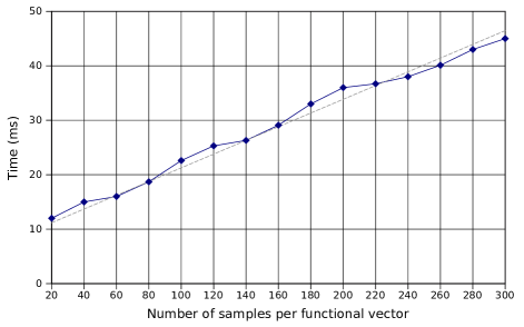
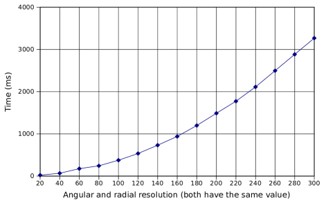
The datasets analyzed in this paper have been processed using sequential extraction of $\xi(\phi,\rho)$ and bilinear interpolation. In order to give an idea of the time spent in a real execution, performance tests have been carried out using a computer with an Intel Core i7-740QM processor at 1.73GHz and 8GB RAM. For Corel 1000, the average time to perform the trace transform of each of the images is 42ms with $n_{\phi}=71$, $n_{\rho}=71$ and $n_{\xi(L)}=251$. There is a very low variance in this processing time as once the parameters are set, this mode of performing the trace transform does not depend on the input image resolution. In the case of Geoeye, the average time is 21ms and the parameters employed $n_{\phi}=51$, $n_{\rho}=71$ and $n_{\xi(L)}=151$. Figure 16 shows the behavior of the trace transform implementation for different values of ($n_{\phi},n_{\rho},n_{\xi(L)}$).

(a) $n_{\xi_{(}L)}$

(b) $n_{\rho}=n_{\phi}$

Figure 16: Time performance behavior depending on applied sampling parameters. Experiments have been carried out using a computer with an Intel Core i7-740QM processor at 1.73GHz and 8GB RAM

4.2 Computational complexity of attribute selection and classification

Attribute selection process is the most computationally expensive task of the process. The training time for Corel 1000 and Geoeye datasets is under one second (609ms average for Corel 1000 and 370ms for Geoeye) and the classification time per sample is around 1$\mu$s.

The attribute selection task can last for some hours and as part of the training process, this fact can lead to strong limitations for some specific uses. Therefore, it can be cut down (as an iterative optimization process, it can interrupted at any point) or even removed. Experimental tests have demonstrated that the attribute selection process can improve the final accuracy by up to 10%.

4.3 Scalability

Each of the datasets used during the validation process contains around 1,000 items. The scalability of the presented framework to larger datasets can be carried out by parallelizing the most critical part of the process which is the trace transform. In fact, the calculation of each functional can be independently executed as it is demonstrated by Meena et al. [64] where an implementation on FPGA of the trace transform operator obtained a throughput of 2725 images per second.

5 Conclusion

We have shown that the DITEC method provides highly discriminant features for context categorization purposes that can be encoded as considerably short feature vectors. We have presented the geometrical constraints of the trace transform that can be optimized to efficiently represent the information contained in the original images. We also have demonstrated that the dimensionality reduction in terms of mean and kurtosis value pair of frequency coefficients results in a very robust set of features in terms of precision. For most resolution ($n_{\phi},n_{\rho},L(n)$) settings maintaining acceptable coverage, homogeneity and redundancy conditions, the accuracy has maintained around 82% for the Corel 1000 dataset and 92% for Geoeye.

Moreover, the method has successfully identified visual similarities within the datasets, and as seen in the validation section, some incorrectly classified instances are in fact visually similar to those pointed out by the classifier. The error analysis has also shown some semantic proximity between visually similar categories, a fact that can be used for context modeling and automatic ontology building.

Igor García Olaizola is the head of Digital TV and Multimedia Services Department in Vicomtech (http://www.vicomtech.org). He received his MEng degree in Electronic and Control Engineering from the University of Navarra, Spain (2001). He developed his Master thesis at Fraunhofer Institut für Integrierte Schaltungen (IIS), Erlangen -Germany- 2001 and currently he is preparing his PhD in Computing Science and Artificial Intelligence at University of Basque Country. He has participated in many industrial projects related with Digital TV as well as several European research projects in the area of audiovisual content management. His current research interests include multimedia content analysis frameworks and techniques to decrease the semantic gap.

Marco Quartulli Marco Quartulli Marco Quartulli received the laurea degree in physics from the University of Bari, Italy, in 1997 and a PhD in EE and CS from the University of Siegen, Germany, in 2005. He worked from 1997 to 2010 on remote sensing ground segment engineering, image analysis, archives and mining for Advanced Computer Systems, Italy. From 2000 to 2003, he was with the Image Analysis Group at the Remote Sensing Technology Institute of the German Aerospace Center (DLR) in Germany. Since 2010, he has joined the Digital Television department of Vicomtech in Spain. His research interests include multimedia mining and asset management, multiple acquisition high-resolution optical and radar remote sensing, scene understanding, data fusion and Bayesian modeling.

Julián Flórez Dr. Julián Flórez studied Industrial Engineering in the University of Navarra (1980), and obtained his Ph.D. in the University of Manchester, Institute of Science and Technology UMIST (1985), in the field of Adaptive Control. From 1985 to 1990, he worked as Researcher in the Centre of Study and Technical Research of Gipuzkoa (CEIT), where he collaborated in several research projects related to Electrical and Industrial Engineering with a marked industrial focus. From 1985 to 1994, he was Associate Professor in the School of Industrial Engineering of the University of Navarra, and since 1994, he is Professor at the same university. From 1990 to 1997, Dr. Flórez worked as Senior Researcher in CEIT, where he was in charge of a Department of Industrial Applications. From 1997 to 2001, he worked as Director of Corporate Development of Avanzit-SGT (Servicios Generales de Teledifusión) in the fields of Information Systems, Communications and Broadcasting infrastructure. He has a strong background in Digital Television infrastructures and was tightly involved in the deployment of one of the biggest Digital TV organizations in Spain and Europe: Quiero TV. Since 2001, he is Principal Researcher in Vicomtech. He holds some patents and has written more than 40 research papers in different areas of Industrial and Electrical Engineering.

Basilio Sierra is Full Professor in the Computer Sciences and Artificial Intelligence Department at the University of the Basque Country. He received his BSc in Computer Sciences in 1990, MSc in Computer Science and Architecture in 1992 and PhD in Computer Sciences in 2000 at the University of the Basque Country. He is the director of the Robotics and Autonomous Systems Group in Donostia-San Sebastian. Professor Sierra is presently a researcher in the fields of Robotics, Computer Vision and Machine Learning, and he is working on the development of different paradigms to improve classification behaviors; he has written more than 25 journal papers in those fields, as well as more than 100 conference contributions and more than 30 book chapters.

References

- [1] T. M. Strat and M. A. Fischler, “Context-based vision: recognizing objects using information from both 2 d and 3 d imagery,” IEEE Transactions on Pattern Analysis and Machine Intelligence, vol. 13, no. 10, pp. 1050–1065, 1991.
- [2] A. Torralba and P. Sinha, “Statistical context priming for object detection,” in Proceedings of the IEEE International Conference on Computer Vision (ICCV), 2001. [Online]. Available: http://web.mit.edu/torralba/www/iccv2001.pdf
- [3] A. Torralba, K. P. Murphy, and W. T. Freeman, “Using the forest to see the trees: exploiting context for visual object detection and localization,” Commun. ACM, vol. 53, no. 3, pp. 107–114, Mar. 2010. [Online]. Available: http://doi.acm.org/10.1145/1666420.1666446
- [4] A. W. M. Smeulders, M. Worring, S. Santini, A. Gupta, and R. Jain, “Content-based image retrieval at the end of the early years,” IEEE Trans. Pattern Anal. Mach. Intell., vol. 22, no. 12, pp. 1349–1380, Dec. 2000. [Online]. Available: http://dx.doi.org/10.1109/34.895972
- [5] G. Marcos, K. Alonso, I. G. Olaizola, J. Florez, and A. Illarramendi, “Dms-1 driven data model to enable a semantic middleware for multimedia information retrieval in a broadcaster,” in Proc. 4th Int. Workshop Semantic Media Adaptation and Personalization SMAP ’09, 2009, pp. 33–37.
- [6] P. J. Haas, “Sketches get sketchier,” Commun. ACM, vol. 54, pp. 100–100, August 2011. [Online]. Available: http://doi.acm.org/10.1145/1978542.1978565
- [7] P. Li and C. König, “b-bit minwise hashing,” in Proceedings of the 19th international conference on World wide web, ser. WWW ’10. New York, NY, USA: ACM, 2010, pp. 671–680. [Online]. Available: http://doi.acm.org/10.1145/1772690.1772759
- [8] C. G. M. Snoek and A. W. M. Smeulders, “Visual-concept search solved?” Computer, vol. 43, no. 6, pp. 76–78, 2010.
- [9] J. C. van Gemert, C. J. Veenman, A. W. M. Smeulders, and J.-M. Geusebroek, “Visual word ambiguity,” IEEE Transactions on Pattern Analysis and Machine Intelligence, vol. 32, no. 7, pp. 1271–1283, 2010.
- [10] D. G. Lowe, “Object recognition from local scale-invariant features,” in Proceedings of the IEEE International Conference on Computer Vision (ICCV), vol. 2. Ieee, 1999, pp. 1150–1157. [Online]. Available: http://ieeexplore.ieee.org/xpls/abs_all.jsp?arnumber=790410
- [11] H. Bay, T. Tuytelaars, and L. V. Gool, “Surf: Speeded up robust features,” in In ECCV, 2006, pp. 404–417.
- [12] A. Rabinovich, A. Vedaldi, C. Galleguillos, E. Wiewiora, and S. Belongie, “Objects in context,” in Proceedings of the IEEE International Conference on Computer Vision (ICCV), 2007, pp. 1–8.
- [13] M. J. Choi, J. J. Lim, A. Torralba, and A. S. Willsky, “Exploiting hierarchical context on a large database of object categories,” in Proc. IEEE Conf. Computer Vision and Pattern Recognition (CVPR), 2010, pp. 129–136.
- [14] I. G. Olaizola, G. Marcos, P. Kramer, J. Florez, and B. Sierra, “Architecture for semi-automatic multimedia analysis by hypothesis reinforcement,” in Proc. IEEE Int. Symp. Broadband Multimedia Systems and Broadcasting BMSB ’09, 2009, pp. 1–6.
- [15] W. Scheirer, N. Kumar, P. Belhumeur, and T. Boult, “Multi-attribute spaces: Calibration for attribute fusion and similarity search,” in Computer Vision and Pattern Recognition (CVPR), 2012 IEEE Conference on, 2012, pp. 2933–2940.
- [16] M. A. Bouker and E. Hervet, “Retrieval of images using mean-shift and gaussian mixtures based on weighted color histograms,” in Proc. Seventh Int Signal-Image Technology and Internet-Based Systems (SITIS) Conf, 2011, pp. 218–222.
- [17] E. Shechtman and M. Irani, “Matching local self-similarities across images and videos,” in Proc. IEEE Conf. Computer Vision and Pattern Recognition CVPR ’07, 2007, pp. 1–8.
- [18] A. Oliva and A. Torralba, “Modeling the shape of the scene: A holistic representation of the spatial envelope,” International Journal of Computer Vision, vol. 42, pp. 145–175, 2001.
- [19] A. Torralba, R. Fergus, and Y. Weiss, “Small codes and large image databases for recognition,” in Proc. IEEE Conf. Computer Vision and Pattern Recognition CVPR, 2008, pp. 1–8.
- [20] T. Watanabe, K. Sugawara, and H. Sugihara, “A new pattern representation scheme using data compression,” IEEE Transactions on Pattern Analysis and Machine Intelligence, vol. 24, no. 5, pp. 579–590, 2002.
- [21] S. Ahmed, M. Khan, and M. Shahjahan, “A filter based feature selection approach using lempel ziv complexity,” in Advances in Neural Networks ISNN 2011, ser. Lecture Notes in Computer Science, D. Liu, H. Zhang, M. Polycarpou, C. Alippi, and H. He, Eds. Springer Berlin / Heidelberg, 2011, vol. 6676, pp. 260–269, 10.1007/978-3-642-21090-7_31. [Online]. Available: http://dx.doi.org/10.1007/978-3-642-21090-7_31
- [22] D. Cerra, A. Mallet, L. Gueguen, and M. Datcu, “Algorithmic information theory-based analysis of earth observation images: An assessment,” IEEE_J_GRSL, vol. 7, no. 1, pp. 8–12, 2010.
- [23] M. R. Mustaffa, F. Ahmad, R. Mahmod, and S. Doraisamy, “Generalized ridgelet-fourier for mxn images: Determining the normalization criteria,” in Proc. IEEE Int Signal and Image Processing Applications (ICSIPA) Conf, 2009, pp. 380–384.
- [24] M. R. Mustaffa, F. Ahmad, R. Mahmod, and s. Doraisamy, “Invariant generalised ridgelet-fourier for shape-based image retrieval,” in Proc. Int Information Retrieval & Knowledge Management, (CAMP) Conf, 2010, pp. 79–84.
- [25] H. Nemmour and Y. Chibani, “Handwritten arabic word recognition based on ridgelet transform and support vector machines,” in High Performance Computing and Simulation (HPCS), 2011 International Conference on, july 2011, pp. 357 –361.
- [26] J. M. Martinez, MPEG-7 Overview, ISO/IEC JTC1/SC29/WG11 Std., Rev. 10, October 2004. [Online]. Available: http://mpeg.chiariglione.org/standards/mpeg-7/mpeg-7.htm
- [27] M. Bober and R. Oami, “Description of mpeg-7 visual core experiments,” ISO/IEC JTC1/SC29/WG11, Tech. Rep., 2007.
- [28] R. O’Callaghan, M. Bober, and P. Oami, R. and. Brasnett, Information technology - Multimedia content description interface - Part 3: Visual, AMENDMENT 3: Image signature tools, ISO/IEC Std. ISO/IEC TC JTC1/SC 29/WG 11 N 9581, 01 2008.
- [29] S. A. Fahmy, “Investigating trace transform architectures for face authentication,” in Proc. Int. Conf. Field Programmable Logic and Applications FPL ’06, 2006, pp. 1–2.
- [30] S. Srisuk, M. Petrou, W. Kurutach, and A. Kadyrov, “Face authentication using the trace transform,” in Proc. IEEE Computer Society Conf. Computer Vision and Pattern Recognition, vol. 1, 2003.
- [31] N. Liu and H. Wang, “Recognition of human faces using siscrete cosine transform filtered trace features,” in Proc. 6th Int Information, Communications & Signal Processing Conf, 2007, pp. 1–5.
- [32] n. Liu and h. Wang, “Modeling images with multiple trace transforms for pattern analysis,” IEEE J SPL, vol. 16, no. 5, pp. 394–397, 2009.
- [33] M. F. Nasrudin, M. Petrou, and L. Kotoulas, “Jawi character recognition using the trace transform,” in Proc. Seventh Int Computer Graphics, Imaging and Visualization (CGIV) Conf, 2010, pp. 151–156.
- [34] J. Turan, Z. Bojkovic, P. Filo, and L. Ovsenik, “Invariant image recognition experiment with trace transform,” in Proc. 7th Int Telecommunications in Modern Satellite, Cable and Broadcasting Services Conf, vol. 1, 2005, pp. 189–192.
- [35] A. Kadyrov and M. Petrou, “The trace transform and its applications,” IEEE Transactions on Pattern Analysis and Machine Intelligence, vol. 23, no. 8, pp. 811–828, 2001.
- [36] J. Li, S. K. Zhou, and R. Chellappa, “Appearance modeling using a geometric transform.” IEEE Trans Image Process, vol. 18, no. 4, pp. 889–902, Apr 2009. [Online]. Available: http://dx.doi.org/10.1109/TIP.2008.2011381
- [37] C. Poynton, A technical introduction to digital video. J. Wiley, 1996. [Online]. Available: http://books.google.es/books?id=jI5jQgAACAAJ
- [38] A. Kadyrov and M. Petrou, “The trace transform as a tool to invariant feature construction,” in Proc. Fourteenth Int Pattern Recognition Conf, vol. 2, 1998, pp. 1037–1039.
- [39] M. Petrou and A. Kadyrov, “Affine invariant features from the trace transform,” IEEE Transactions on Pattern Analysis and Machine Intelligence, vol. 26, no. 1, pp. 30–44, 2004.
- [40] P. Brasnett and M. Bober, “Fast and robust image identification,” in Proc. 19th Int. Conf. Pattern Recognition ICPR 2008, 2008, pp. 1–5.
- [41] F. Peyrin and R. Goutte, “Image invariant via the radon transform,” in Proc. Int Image Processing and its Applications Conf, 1992, pp. 458–461.
- [42] S. Lin, S. Li, and C. Li, “A fast electronic components orientation and identify method via radon transform,” in Proc. IEEE Int Systems Man and Cybernetics (SMC) Conf, 2010, pp. 3902–3908.
- [43] J. S. Seo, J. Haitsma, T. Kalker, and C. D. Yoo, “A robust image fingerprinting system using the radon transform,” Sig. Proc.: Image Comm., vol. 19, no. 4, pp. 325–339, 2004.
- [44] R. Fooprateepsiri, W. Kurutach, and S. Tamsumpaolerd, “An image identifier based on hausdorff shape trace transform,” in Proceedings of the 16th International Conference on Neural Information Processing: Part I, ser. ICONIP ’09. Berlin, Heidelberg: Springer-Verlag, 2009, pp. 788–797. [Online]. Available: http://dx.doi.org/10.1007/978-3-642-10677-4_90
- [45] A. Kadyrov and M. Petrou, “Affine parameter estimation from the trace transform,” IEEE Transactions on Pattern Analysis and Machine Intelligence, vol. 28, no. 10, pp. 1631–1645, 2006.
- [46] Z. Shi, M. Du, and R. Huang, “A trace transform based on subspace method for face recognition,” in Proc. Int Computer Application and System Modeling (ICCASM) Conf, vol. 13, 2010.
- [47] J. E. Bresenham, “Algorithm for computer control of a digital plotter,” IBM Systems journal, vol. 4, no. 1, pp. 25–30, 1965. [Online]. Available: http://ieeexplore.ieee.org/xpls/abs_all.jsp?arnumber=5388473
- [48] N. Ahmed, T. Natarajan, and K. R. Rao, “Discrete cosine transform,” IEEE-J-C, no. 1, pp. 90–93, 1974.
- [49] I. E. Richardson, Video Codec Design: Developing Image and Video Compression Systems. New York, NY, USA: John Wiley & Sons, Inc., 2002.
- [50] T. M. Mitchell, Machine Learning, 1st ed. New York, NY, USA: McGraw-Hill, Inc., 1997.
- [51] H. Liu and H. Motoda, Feature Selection for Knowledge Discovery and Data Mining. Kluwer Academic Publishers, 1998.
- [52] I. Inza, P. Larrañaga, and B. S. R. Etxeberria, “Feature subset selection by Bayesian networks based optimization,” Artificial Intelligence, vol. 123, no. 1–2, pp. 157–184, 2000.
- [53] R. Blanco, P. Larrañaga, I. Inza, and B. Sierra, “Gene selection for cancer classification using wrapper approaches,” International Journal of Pattern Recognition and Artificial Intelligence, 2004.
- [54] B. Sierra, E. Lazkano, E. Jauregi, and I. Irigoien, “Histogram distance-based bayesian network structure learning: A supervised classification specific approach,” Decision Support Systems, vol. 48, no. 1, pp. 180–190, 2009.
- [55] D. Meyer, F. Leisch, , and K. Hortnik, “The support vector machine under test,” Neurocomputing, vol. 55, pp. 169–186, 2003.
- [56] N. Kumar, A. C. Berg, P. N. Belhumeur, and S. K. Nayar, “Describable visual attributes for face verification and image search,” IEEE Trans. Pattern Anal. Mach. Intell., vol. 33, no. 10, pp. 1962–1977, 2011.
- [57] F. Dornaika, E. Lazkano, and B. Sierra, “Improving dynamic facial expression recognition with feature subset selection,” Pattern Recognition Letters, vol. 32, no. 5, pp. 740 – 748, 2011. [Online]. Available: http://www.sciencedirect.com/science/article/pii/S0167865510004071
- [58] G. Dalley and P. Flynn, “Pair-wise range image registration: A study in outlier classification,” Computer Vision and Image Understanding, vol. 87, no. 1-3, pp. 104 – 115, 2002. [Online]. Available: http://www.sciencedirect.com/science/article/pii/S1077314202909860
- [59] [Online]. Available: http://wang.ist.psu.edu/docs/related.shtml
- [60] M. Jacomy, S. Heymann, T. Venturini, and M. Bastian, “Forceatlas2, a graph layout algorithm for handy network visualization,” Gephi – Web Atlas, Draft, 2011. [Online]. Available: http://webatlas.fr/tempshare/ForceAtlas2_Paper.pdf
- [61] G. Zajic, N. Kojic, N. Reljin, and B. Reljin, “Experiment with reduced feature vector in cbir system with relevance feedback,” IET Conference Publications, vol. 2008, no. CP543, pp. 176–181, 2008. [Online]. Available: http://link.aip.org/link/abstract/IEECPS/v2008/iCP543/p176/s1
- [62] W. Bouachir, M. Kardouchi, and N. Belacel, “Fuzzy indexing for bag of features scene categorization,” in Proc. 5th Int I/V Communications and Mobile Network (ISVC) Symp, 2010, pp. 1–4.
- [63] [Online]. Available: http://www.geoeye.com
- [64] M. Meena, K. Pramod, and K. Linganagouda, “Optimized trace transform based feature extraction architecture for cbir,” in Advances in Computing and Communications, ser. Communications in Computer and Information Science, A. Abraham, J. Mauri, J. Buford, J. Suzuki, and S. Thampi, Eds. Springer Berlin Heidelberg, 2011, vol. 192, pp. 444–451. [Online]. Available: http://dx.doi.org/10.1007/978-3-642-22720-2_46
![[Uncaptioned image]](/html/1208.3901/assets/images/iolaizola.jpg) |