A study on the interacting Ricci dark energy in $f(R,T)$ gravity

Abstract

The present work reports study on the interacting Ricci dark energy in a modified gravity theory named $f(R,T)$ gravity. The specific model $f(R,T)=\mu R+\nu T$ (proposed by R. Myrzakulov, arXiv:1205.5266v2 Myrza1 ) is considered here. For this model we have observed a quintom-like behavior of the equation of state (EoS) parameter and a transition from matter dominated to dark energy density has been observed through fraction density evolution. The statefinder parameters reveal that the model interpolates between dust and $\Lambda$CDM phases of the universe.

I Introduction

The origin of dark energy (for review see Copeland ; Paddy ; BambaOdintsov ) responsible for the cosmic acceleration Spergel ; Perlmu is one of the most serious problems in modern cosmology. The first step toward understanding the nature of dark energy is to clarify whether it is a simple cosmological constant or it originates from other sources that dynamically change in time Tsuza . In an extensive review, Nojiri and Odintsov Nojiri1 thoroughly discussed the reasons why modified gravity approach is extremely attractive in the applications for late accelerating universe and dark energy. Other remarkable reviews on modified gravity are Clifton ; Tsuza . Various modified gravity theories have been proposed so far. These include, $f(R)$ Nojiri2 ; Nojiri3 , $f(T)$ Cai1 ; Ferraro ; Bamba1 ; BambaGeng , $f(G)$ Myrza2 ; Setare1 , Horava-Lifshitz Kiritsis ; Nishioka and Gauss-Bonnet Nojiri4 ; Li theories. The present work concentrates on $f(R,T)$ gravity, with $T$ being the trace of stress-energy tensor, manifesting a coupling between matter and geometry. Before going into the details of $f(R,T)$ gravity, let us first briefly survey the $f(R)$ gravity. The recent motivation for studying $f(R)$ gravity has come from the necessity to explain the apparent late-time accelerating expansion of the Universe Clifton . Some extensive reviews of $f(R)$ gravity are Soti ; Antonio ; Soti1 ; Capoz . Thermodynamic aspects of $f(R)$ gravity have been investigated in the works of Bambathermo ; Akbar . A generalization of $f(R)$ modified theories of gravity including in the theory an explicit coupling of an arbitrary function of the Ricci scalar $R$ with the matter Lagrangian density $\mathcal{L}_{m}$ leads to the motion of the massive particles is non-geodesic, and an extra force, orthogonal to the four-velocity, arises Nojiri5 ; Papa . Harko et al Nojiri5 proposed an extension of standard general relativity, where the gravitational Lagrangian is given by an arbitrary function of the Ricci scalar $R$ and of the trace of the stress-energy tensor $T$ and dubbed this as $f(R,T)$ gravity. The $f(R,T)$ gravity model depends on a source term, representing the variation of the matter stress-energy tensor with respect to the metric. A general expression for this source term is obtained as a function of the matter Lagrangian $\mathcal{L}_{m}$ Nojiri5 . In a recent paper, Myrzakulov Myrza1 derived exact solutions for a specific model $f(R,T)=\mu R+\nu T$ and showed that for some values of the parameters the expansion of our universe can be accelerated without introducing any dark component. The present work aims to reconstruct the Ricci dark energy (RDE) Gao ; Kim ; Feng ; Fu ; Xu under $f(R,T)$ gravity. Rest of the work is organized as follows: In section II we have briefly reviewed RDE. In section III we have presented an overview of $f(R,T)$ gravity. In section IV we have reconstructed interacting RDE in $f(R,T)$ gravity. We have concluded in section V.

II A brief overview of Ricci dark energy

Gao et.al Gao proposed a holographic dark energy model in which the future event horizon is replaced by the inverse of the Ricci scalar curvature, and dubbed this model the “Ricci dark energy model”(RDE). This model (i) avoids the causality problem (ii) is phenomenologically viable, and (iii) can solve the coincidence problem of dark energy Feng . The Ricci curvature of FRW universe is given by Feng

$$R=-6\left(\dot{H}+2H^{2}+\frac{k}{a^{2}}\right)$$ (1)

where, $k$ is the curvature of the universe and $a$ is the scale factor. The energy density of RDE is given by Feng1

$$\rho_{X}=3c^{2}\left(\dot{H}+2H^{2}+\frac{k}{a^{2}}\right)$$ (2)

In flat FRW universe, $k=0$ and hence we have

$$\rho_{X}=3c^{2}\left(\dot{H}+2H^{2}\right)$$ (3)

In the present work we are considering RDE interacting with pressureless dark matter with energy density $\rho_{m}$. Various forms of “interacting” dark energy models have been constructed in order to fulfil the observational requirements. Plethora of literatures are available where the interacting dark energies have been discussed. Several examples of interacting dark energy are presented in Jamil ; Wu ; Kim ; Setare ; Wang ; Karami . In a subsequent section we shall consider the interacting RDE in $f(R,T)$ gravity. The metric of a spatially flat homogeneous and isotropic universe in FRW model is given by

$$ds^{2}=dt^{2}-a^{2}(t)\left[dr^{2}+r^{2}(d\theta^{2}+sin^{2}\theta d\phi^{2})\right]$$ (4)

where $a(t)$ is the scale factor. The Einstein field equations are given by

$$H^{2}=\frac{1}{3}\rho$$ (5)

and

$$\dot{H}=-\frac{1}{2}(\rho+p)$$ (6)

where $\rho$ and $p$ are energy density and isotropic pressure respectively (choosing $8\pi G=c=1$). The conservation equation is given by

$$\dot{\rho}+3H(\rho+p)=0$$ (7)

As we are considering interaction between RDE and dark matter,

$$\rho=\rho_{X}+\rho_{m},~{}~{}p=p_{X}$$ (8)

It should be stated that we are considering pressureless dark matter, $p_{m}=0$. Since the components do not satisfy the conservation equation separately in the case of interaction, we need to reconstruct the conservation equation by introducing an interaction term $Q$. The interaction term could be in any of the forms sheykhi : $Q\propto H\rho_{X}$, $Q\propto H\rho_{m}$ and $Q\propto H(\rho_{X}+\rho_{m})$. In the present paper we take the interaction term in the second of the three forms mentioned above. Accordingly the conservation equation is reconstructed as

$$\dot{\rho}_{X}+3H(\rho_{X}+p_{X})=3H\delta\rho_{m}$$ (9)

$$\dot{\rho}_{m}+3H\rho_{m}=-3H\delta\rho_{m}$$ (10)

III The $f(R,T)$ model

One of interesting models of $f(R,T)$ gravity is the so-called $M_{37}$-model. Its action is Myrza1

$$S=\int f(R,T)\sqrt{-g}d^{4}x+\int\mathcal{L}_{m}\sqrt{-g}d^{4}x$$ (11)

where $\mathcal{L}_{m}$ is the matter Lagrangian and $f(R,T)$ is an arbitrary function of $R$ and $T$, where $R$ is the scalar curvature and $T$ is the torsion scalar. Here,

$$R=u+6(\dot{H}+2H^{2})$$ (12)

$$T=v-6H^{2}$$ (13)

Ref Myrza1 considered the following model of $f(R,T)$

$$f(R,T)=\mu R+\nu T$$ (14)

where $\mu$ and $\nu$ are real constants and $u$ and $v$ are taken as $u=\alpha a^{n}$ and $v=\beta a^{m}$ with $m,~{}n,~{}\alpha$ and $\beta$ as real constants. The equations system of this $f(R,T)$ is

$$\mu D_{1}+\nu E_{1}+K(\nu T+\mu R)=-2a^{3}\rho$$ (15)

$$\mu A_{1}+\nu B_{1}+M(\nu T+\mu R)=6a^{2}p$$ (16)

$$\dot{\rho}+3H(\rho+p)=0$$ (17)

where,

$$D_{1}=a^{3}\left(6\frac{\ddot{a}}{a}+\dot{a}u_{\dot{\alpha}}\right)$$ (18)

$$E_{1}=a^{3}\left(-12\frac{\dot{a}^{2}}{a^{2}}+\dot{a}v_{\dot{\alpha}}\right)$$ (19)

$$K=-a^{3}$$ (20)

$$A_{1}=12\dot{a}^{2}+6a\ddot{a}+3a^{2}\dot{a}u_{\dot{\alpha}}+a^{3}\dot{u}_{\dot{\alpha}}-a^{3}u_{\alpha}$$ (21)

$$B_{1}=-24\dot{a}^{2}-12a\ddot{a}+3a^{2}\dot{a}v_{\dot{\alpha}}+a^{3}\dot{v}_{\dot{\alpha}}-a^{3}v_{\alpha}$$ (22)

$$M=-3a^{2}$$ (23)

$$R=u+6(\dot{H}+2H^{2})$$ (24)

$$T=v-6H^{2}$$ (25)

Subsequently, the modified field equations are obtained as Myrza1

$$3(\mu+\nu)H^{2}+\frac{1}{2}(\mu\alpha a^{n}+\nu\beta a^{m})=\rho$$ (26)

$$(\mu+\nu)(2\dot{H}+3H^{2})+\frac{\mu\alpha(n+3)}{6}a^{n}+\frac{\nu\beta(m+3)}{6}a^{m}=-p$$ (27)

IV Interacting RDE in the $f(R,T)$ gravity

As stated earlier, $\rho=\rho_{X}+\rho_{m}$ and $p=p_{X}$ are taken in the equations (26) and (27). From equation (10) we get

$$\rho_{m}=\rho_{m0}a^{-3(1+\delta)}$$ (28)

Using equations (3) and (28) in the right hand side of the equation (26) we get the Hubble’s parameter as a function of the scale factor $a$ as

$$H^{2}=C_{1}a^{\frac{2(-2c^{2}+\mu+\nu)}{c^{2}}}+\frac{1}{3a^{3}}\left[\frac{\alpha\mu a^{3+m}}{c^{2}(4+m)-2(\mu+\nu)}+\frac{\beta\nu a^{3+n}}{c^{2}(4+n)-2(\mu+\nu)}+\frac{2a^{-3\delta}\rho_{m0}}{c^{2}(-1+3\delta)+2(\mu+\nu)}\right]$$ (29)

Subsequently we get $\dot{H}$ and $\ddot{H}$ as functions of $a$ as follows

$$\begin{array}[]{c}\dot{H}=\frac{a^{\frac{2(-2c^{2}+\mu+\nu)}{c^{2}}}C_{1}(-2c^{2}+\mu+\nu)}{c^{2}}\\ +\frac{a^{m}m\alpha\mu}{6(c^{2}(4+m)-2(\mu+\nu))}+\frac{a^{n}n\beta\nu}{6(c^{2}(4+n)-2(\mu+\nu))}-\frac{a^{-3(1+\delta)(1+\delta)\rho_{m0}}}{c^{2}(-1+3\delta)+2(\mu+\nu)}\\ \end{array}$$ (30)

$$\begin{array}[]{c}\ddot{H}=\frac{H}{6a^{4}}\left[\frac{12a^{\frac{2(\mu+\nu)}{c^{2}}}C_{1}(-2c^{2}+\mu+\nu)^{2}}{c^{4}}\right.\\ \left.+\frac{a^{4+m}m^{2}\alpha\mu}{c^{2}(4+m)-2(\mu+\delta)}+\frac{a^{4+n}n^{2}\beta\nu}{c^{2}(4+n)-2(\mu+\nu)}+\frac{18a^{1-3\delta}(1+\delta)^{2}\rho_{m0}}{c^{2}(-1+3\delta)+2(\mu+\nu)}\right]\\ \end{array}$$ (31)

Using (29) and (30) in equation (3) we get the energy density for RDE under interaction with pressureless dark matter under $f(R,T)$ gravity as

$$\rho_{X}=\frac{1}{2}\left[6a^{\frac{2(-2c^{2}+\mu+\nu)}{c^{2}}}C_{1}(\mu+\nu)+\frac{a^{m}c^{2}\alpha\mu(4+m)}{c^{2}(4+m)-2(\mu+\nu)}+\frac{a^{n}c^{2}\beta\nu(4+n)}{c^{2}(4+n)-2(\mu+\nu)}-\frac{2a^{-3(1+\delta)}c^{2}(-1+3\delta)\rho_{m0}}{c^{2}(-1+3\delta)+2(\mu+\nu)}\right]$$ (32)

Using the above form of $\rho_{X}$ in the conservation equation (9) we get the pressure for RDE in the present case as

$$\begin{array}[]{c}p_{X}=\frac{1}{6}\left[-a^{n}(3+n)\alpha\mu-a^{m}(3+m)\beta\nu-6(\mu+\nu)\left\{-\frac{a^{\frac{2(-2c^{2}+\mu+\nu)}{c^{2}}}C_{1}(c^{2}-2(\mu+\nu))}{c^{2}}+\right.\right.\\ \left.\left.\frac{a^{m}(3+m)\alpha\mu}{3(c^{2}(4+m)-2(\mu+\nu))}+\frac{a^{n}(3+n)\beta\nu}{3(c^{2}(4+n)-2(\mu+\nu))}-\frac{2a^{-3(1+\delta)}\delta\rho_{m0}}{c^{2}(-1+3\delta)+2(\mu+\nu)}\right\}\right]\\ \end{array}$$ (33)

Using the expressions for energy density and pressure derived above we get the equation of state parameters

$$w_{X}=\frac{p_{X}}{\rho_{X}}$$ (34)

and

$$w_{total}=\frac{p_{X}}{\rho_{X}+\rho_{m}};~{}~{}(p_{m}=0)$$ (35)

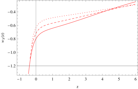
Figure 1: Behavior of $w_{X}=\frac{p_{X}}{\rho_{X}}$ against redshift $z=a^{-1}-1$.

Figure 2: Behavior of $w_{total}=\frac{p_{X}}{\rho_{X}+\rho_{m}}$.

The deceleration parameter $q$ Gong comes out to be

$$q=-\frac{a\ddot{a}}{\dot{a}^{2}}=-1-\frac{\dot{H}}{H^{2}}=-1-\frac{\zeta_{1}}{\zeta_{2}}$$ (36)

where,

$$\zeta_{1}=\frac{6a^{2(-2c^{2}+\mu+\nu)}C_{1}(-2c^{2}+\mu+\nu)}{c^{2}}+\frac{a^{m}m\alpha\mu}{c^{2}(4+m)-2(\mu+\nu)}+\frac{a^{n}n\beta\nu}{c^{2}(4+n)-2(\mu+\nu)}-\frac{6a^{-3(1+\delta)}(1+\delta)\rho_{m0}}{c^{2}(-1+3\delta)+2(\mu+\nu)}$$ (37)

$$\zeta_{2}=2\left(3a^{\frac{2(-2c^{2}+\mu+\nu)}{c^{2}}}C_{1}+\frac{a^{m}m\alpha\mu}{c^{2}(4+m)-2(\mu+\nu)}+\frac{a^{n}\beta\nu}{c^{2}(4+n)-2(\mu+\nu)}+\frac{2a^{-3(1+\delta)}\rho_{m0}}{c^{2}(-1+3\delta)+2(\mu+\nu)}\right)$$ (38)

Next, we consider the statefinder parameters $\{r,s\}$ Sahni for the present case. Using equations (29), (30) and (31) we get the statefinder parameters as

$$r=1+3\frac{\dot{H}}{H^{2}}+\frac{\ddot{H}}{H^{3}}=1+\frac{\varrho_{1}}{\varrho_{2}}$$ (39)

$$\begin{array}[]{c}\varrho_{1}=\frac{6a^{\frac{2(-2c^{2}+\mu+\nu)}{c^{2}}}C_{1}\{2c^{4}-5c^{2}(\mu+\nu)+2(\mu+\nu)^{2}\}}{c^{4}}\\ +\frac{a^{m}m(3+m)\alpha\mu}{(c^{2}(4+m)-2(\mu+\nu))}+\frac{a^{n}n(3+n)\beta\nu}{(c^{2}(4+n)-2(\mu+\nu))}-\frac{18a^{-3(1+\delta)}(1+\delta)\delta\rho_{m0}}{c^{2}(-1+3\delta)+2(\mu+\nu)}\\ \end{array}$$ (40)

$$\begin{array}[]{c}\varrho_{2}=2\left[3C_{1}a^{\frac{2(-2c^{2}+\mu+\nu)}{c^{2}}}+\frac{1}{a^{3}}\left\{\frac{\alpha\mu a^{3+m}}{c^{2}(4+m)-2(\mu+\nu)}+\right.\right.\\ \left.\left.\frac{\beta\nu a^{3+n}}{c^{2}(4+n)-2(\mu+\nu)}+\frac{2a^{-3\delta}\rho_{m0}}{c^{2}(-1+3\delta)+2(\mu+\nu)}\right\}\right]\\ \end{array}$$ (41)

$$s=-\frac{3H\dot{H}+\ddot{H}}{3H(2\dot{H}+3H^{2})}=\frac{\xi_{1}}{\xi_{2}}$$ (42)

where,

$$\begin{array}[]{c}\xi_{1}=-\left(\frac{a^{m}m(3+m)\alpha\mu}{6(c^{2}(4+m)-2(\mu+\nu))}+\frac{a^{n}n(3+n)\beta\nu}{6(c^{2}(4+n)-2(\mu+\nu))}\right.\\ \left.+\frac{1}{c^{4}}a^{\frac{2(-2c^{2}+\mu+\nu)}{c^{2}}}C_{1}(2c^{4}-5c^{2}(\mu+\nu)+2(\mu+\nu)^{2})+\frac{3a^{-3(1+\delta)}\delta(1+\delta)\rho_{m0}}{c^{2}(-1+3\delta)+2(\mu+\nu)}\right)\\ \end{array}$$ (43)

$$\begin{array}[]{c}\xi_{2}=3\left(-\frac{1}{c^{2}}a^{\frac{2(-2c^{2}+\mu+\nu)}{c^{2}}}+\frac{a^{m}(3+m)\alpha\mu}{3(c^{2}(4+m)-2(\mu+\nu))}\right.\\ \left.+\frac{a^{n}(3+n)\beta\nu}{3(c^{2}(4+n)-2(\mu+\nu))}-\frac{2a^{-3(1+\delta)}\delta\rho_{m0}}{c^{2}(-1+3\delta)+2(\mu+\nu)}\right)\\ \end{array}$$ (44)

V Discussions

In figure 1 we have presented the EoS parameter $w_{X}=\frac{p_{X}}{\rho_{X}}$ for RDE under $f(R,T)$ gravity against redshift $z=a^{-1}-1$. In this and the subsequent figures the solid, dashed and dotted lines would correspond to $c^{2}<,~{}=,~{}>0.5$ respectively. Figure 1 shows that for all values of $c^{2}$ the EoS parameter transits from $w_{X}>-1$ to $w_{X}<-1$ i.e. from quintessence to phantom. From this figure we see that at early times, roughly $z>2$, the EoS approaches 0; i.e., in this model the dark energy behaves like dust matter during most of the epoch of matter domination. The EoS crosses phantom crossing $w_{X}=-1$ at $z\approx-0.2$ and in the distant future, the equation of state approaches $w_{X}=-1.2$, the Universe evolves into the phantom-dominated epoch. For this model, the EoS crosses $-1$ , so it may be classified as a “quintom”. Thus, the interacting RDE behaves like quintom in the $f(R,T)$ gravity model proposed by Myrza1 . In figure 2 we have plotted $p_{total}=\frac{p_{X}}{\rho_{X}+\rho_{m}}$, where we found similar crossing of the phantom divide $w_{total}=-1$ and transition from $w_{total}>-1$ at higher redshift to $w_{total}<-1$ at lower redshifts. It might be stated that we have chosen the model parameters as $\alpha=1.2,~{}\beta=1.2,~{}\nu=0.3,~{}\mu=0.4,~{}n=3,C_{1}=3.02,~{}\delta=0.05,~{}\rho_{m0}=0.23$ and $m=2$. In all the figures, the solid, dashed and dotted lines correspond to $c^{2}<0.5,~{}=0.5$ and $>0.5$ respectively.

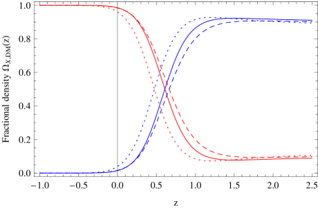
Figure 3: Behavior of fractional densities $\Omega_{X}=\frac{\rho_{X}}{3\tilde{H}^{2}}$ (red lines) and $\Omega_{m}=\frac{\rho_{m}}{3\tilde{H}^{2}}$ (blue lines) with evolution of the universe.

In figure 3 we have plotted fractional densities $\Omega_{X}=\frac{\rho_{X}}{3\tilde{H}^{2}}$ and $\Omega_{m}=\frac{\rho_{m}}{3\tilde{H}^{2}}$ against redshift $z$. where, $\tilde{H}^{2}=(\mu+\nu)H^{2}+\frac{1}{6}(\mu\alpha(1+z)^{-n}+\nu\beta(1+z)^{-m})$. We observe that at from higher to lower redshifts the fractional density $\Omega_{X}$ of RDE is increasing, while the fractional density of dark matter is decreasing. This indicates the transition from the matter dominated to dark energy dominated universe. At very early stage of universe $z>2$, the fractional density of dark energy $\Omega_{X}$ is dominated by fractional density of dark matter $\Omega_{DM}$. After $z=2$, the $\Omega_{X}$ starts showing an increasing pattern and $\Omega_{DM}$ starts showing a decaying pattern. This indicates the gradual transition from matter dominated era to the dark energy dominated era. We denote the cross-over point of the fractional densities by $z_{cross}$, where $\Omega_{X}=\Omega_{DM}$. For $c^{2}<0.5,~{}=0.5$ and $>0.5$ the $z_{cross}\approx 0.6,~{}0.75$ and $0.5$ respectively. It is also observed that in the early universe the density contribution of dark energy can occupy roughly 20$\%$-30$\%$. However, at this stage the dark energy behaves like dust matter. So, effectively speaking, the matter density contribution is still 100$\%$. Finally, from figure 3 our observation is that RDE in $f(R,T)$ gravity is capable of achieving the transition from matter-dominated to dark energy-dominated universe.

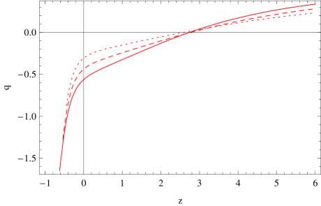
Figure 4: Behavior of deceleration parameter $q$ (Eq. 36).

In figure 4 we have plotted the deceleration parameter $q$ as a function of the redshift $z$. We observe that at very early stage, roughly $z>2$, $q>0$ i.e. the decelerated universe. At $z\approx 2.5$ the deceleration parameter transits from positive to negative level. That is, the universe gradually transits from decelerated to accelerated stage. At later stage $q=-1.5$. Thus, we observe that it is possible to achieve the accelerated phase of the universe from decelerated phase for RDE under $f(R,T)$ gravity.

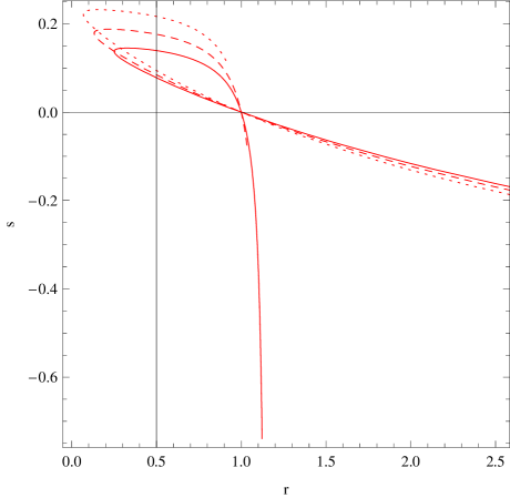
Figure 5: The $r-s$ trajectory (Eqs. 39 and 42).

In figure 5 we have created the $r-s$ trajectories for the three values of $c^{2}$ under consideration. Sahni et al. Sahni demonstrated that the statefinder diagnostic could effectively discriminate different forms of dark energy. Cosmological constant, quintessence, Chaplygin gas, and braneworld models were investigated by Alam using the statefinder diagnostics and it was observed that the statefinder pair could differentiate between these models. An investigation on statefinder parameters for differentiating between dark energy and modified gravity was carried out in Wang1 . Statefinder diagnostics for $f(T)$ gravity has been investigated in WuYu . In the $\{r,s\}$ plane, $s>0$ corresponds to a quintessence like dark energy and $s<0$ corresponds to a phantom-like dark energy, and an evolution from phantom to quintessence or inverse is given by a crossing of the point $(r=1,s=0)$ in $\{r,s\}$ plane WuYu . Also, the fixed point $(r=1,s=0)$ corresponds to $\Lambda$CDM scenario. In figure 5 we clearly observe a transition from quintessence to phantom as the $r-s$ trajectory transits from positive to negative sides of $s$ after crossing the $(r=1,s=0)$ point. Also, we find that, for finite $r$, $s\rightarrow-\infty$ that corresponds to dust phase. Thus, the interacting RDE in $f(,T)$ gravity with $f(R,T)=\mu R+\nu T$ interpolates between dust and $\Lambda$CDM phases of the universe. Also, the statefinder diagnostics supports the quintom-like behavior of the equation of state.

VI Concluding remarks

In this work we considered interacting Ricci dark energy in $f(R,T)=\mu R+\nu T$ gravity. We have observed that the EoS parameter exhibits quintom like behavior for this model. Also, the transition from matter dominated to dark energy dominated universe is achievable by this model. The deceleration parameter have exhibited a transition from positive to negative sign, thereby showing the evolution of the universe from deceleration to acceleration. The statefinder diagnostics have been investigated and an interpolation between dust and $\Lambda$CDM phases of the universe has been observed under this model.

References

(1) E. J. Copeland, M. Sami and S. Tsujikawa, Int. J. Mod. Phys. D 15 1753
(2006).
(2) T. Padmanabhan, Current Science 88 1057 (2005).
(3) K. Bamba, S. Capozziello, S. Nojiri and S. D.
Odintsov, arXiv:1205.3421v3 [gr-qc].
(4) D. N. Spergel et al., Astrophys. J. Suppl. 148 175 (2003).
(5) S. Perlmutter et al., Astrophys. J. 517 565 (1999).
(6) S. Tsujikawa, Lect. Notes Phys. 800 99
(2010).
(7) S. Nojiri and S. D. Odintsov, Int. J. Geom. Meth. Mod. Phys. 4 115
(2007).
(8) T. Clifton, P. G. Ferreira, A. Padilla and C.
Skordis, Physics Reports 513 1 (2012).
(9) S. Nojiri and S. D. Odintsov, Phys. Rev. D 74 086005 (2006).
(10) S. Nojiri and S.D. Odintsov, Phys. Rev. D 77 026007 (2008).
(11) Y-F. Cai, S-H. Chen, J. B. Dent, S. Dutta and E. N.
Saridakis, Class. Quantum Grav. 28 215011 (2011).
(12) R. Ferraro and F. Fiorini, Phys. Rev. D 75 084031
(2007).
(13) K. Bamba, C-Q. Geng, C-C. Lee and L-W. Luo, JCAP 1101 021
(2011).
(14) K. Bamba, C-Q. Geng and Chung-Chi Lee, arXiv:1008.4036v1
[astro-ph.CO].
(15) R. Myrzakulov, D. S aez-G omez and A. Tureanu, Gen. Rel. Grav. 43 1671
(2011).
(16) A. Banijamali, B. Fazlpour and M. R. Setare,
Astrophys. Space Sci. 338 327 (2012).
(17) E. Kiritsis and G. Kofinas, Nucl. Phys. B 821 467
(2009).
(18) T. Nishioka, Class. Quant. Grav. 26 242001
(2009).
(19) S. Nojiri and S. D. Odintsov, Phys. Lett. B 631 1
(2005).
(20) B. Li, J. D. Barrow and D. F. Mota, Phys. Rev. D 76 044027
(2007).
(21) T. P. Sotiriou and V. Faraoni, Rev. Mod. Phys. 82 451
(2010).
(22) A. De Felice and S. Tsujikawa, Living Rev. Rel. 13 3
(2010).
(23) T. P. Sotiriou, Class. Quant. Grav. 23 5117
(2006).
(24) S. Capozziello and M. De Laurentis, Phys. Rept. 509 167
(2011).
(25) K. Bamba and C.-Q. Geng, Phys. Lett. B 679 282
(2009).
(26) M. Akbar and R-G. Cai, Phys. Lett. B 648 243
(2007).
(27) T. Harko, F. S. N. Lobo, S. Nojiri and S. D.
Odintsov, Phys. Rev. D 84 024020 (2011).
(28) N. J. Poplawski, arXiv:gr-qc/0608031v2.
(29) R. Myrzakulov, arXiv:1205.5266v2 (2012).
(30) Gao et al., Phys. Rev. D 79 043511 (2009).
(31) K. Y. Kim, H. W. Lee and Y. S. Myung, Gen. Rel. Grav. 43 1095
(2011).
(32) C-J. Feng, Phys. Lett. B 670 231 (2008).
(33) T-F. Fu, J-F. Zhang, J-Q. Chen and X. Zhang, Eur. Phys. J. C 72 1932
(2012).
(34) L. Xu and Y. Wang, JCAP 06 002 (2010).
(35) C-J. Feng, Phys. Lett. B 676 168 (2009).
(36) M. Jamil, E. N. Saridakis and M.R. Setare, 81 023007
(2010).
(37) Q. Wu et al., Phys. Lett. B 659 34 (2008).
(38) H. Kim, H. W. Lee, and Y. S. Myung, Phys. Lett. B
632 605 (2006).
(39) M. R. Setare, J. Cosmol. Astropart. Phys. 01 023 (2007).
(40) B. Wang, Y.G. Gong, and E. Abdalla, Phys. Lett. B
624 141 (2005).
(41) K. Karami and A. Sorouri, Phys. Scripta 82 025901
(2010).
(42) A. Sheykhi, Phys. Lett. B 682,
329 (2010).
(43) Y. Gong and A. Wang, Phys. Rev. D 75 043520
(2007).
(44) V. Sahni et al., JETP Lett. 77 201 (2003).
(45) U. Alam, V. Sahni, T. D. Saini and A. A. Starobinsky, MNRAS 344
1057 (2003).
(46) F. Y. Wang, Z. G. Dai and S. Qi, Astronomy Astrophysics 507 53 (2009).
(47) P. Wu and H. Yu, Phys. Lett. B 693 415
(2010).