General relativistic null-cone evolutions with a high-order scheme

Abstract

We present a high-order scheme for solving the full non-linear Einstein equations on characteristic null hypersurfaces using the framework established by Bondi and Sachs. This formalism allows asymptotically flat spaces to be represented on a finite, compactified grid, and is thus ideal for far-field studies of gravitational radiation. We have designed an algorithm based on 4th-order radial integration and finite differencing, and a spectral representation of angular components. The scheme can offer significantly more accuracy with relatively low computational cost compared to previous methods as a result of the higher-order discretization. Based on a newly implemented code, we show that the new numerical scheme remains stable and is convergent at the expected order of accuracy.

1 Introduction

Characteristic formulations of the Einstein equations have proven to be an important tool for numerical relativity. Most recently, they have been employed for the practical problem of measuring gravitational waves in a gauge-invariant and unambiguous way from numerically evolved spacetimes of binary black hole mergers [1, 2, 3, 4], rotating stellar core collapse [5], and collapsar formation [6]. The technique, called Cauchy-characteristic extraction (CCE) (see [7] for a review) takes metric boundary data produced by a 3+1 evolution on a worldtube $\Gamma$ of finite radius, and uses null-cone evolutions of the Einstein equations to transport that metric data to future null infinity, $\mathcal{J}^{+}$, the conformal outer boundary of spacetime where gravitational radiation is invariantly defined and interpreted in the Bondi gauge [8, 9, 10]. Thus, this technique removes the influence of near-zone and coordinate effects [1, 2, 3, 4, 5].

The null formulation is extremely efficient for evolving fields in the wave zone, where the null coordinates are well-behaved and caustics along geodesics are unlikely to be an issue. On relatively small computational grids, by comparison with standard 3+1 methods, it is possible to achieve an accuracy which has proven to be sufficient for practical applications (gravitational wave measurement from compact bodies). In the case of characteristic gravitational-wave extraction, the inner boundary data for characteristic evolution is constructed on a worldtube at some distance form the source where the curvature gradients are already rather small compared to those close to the source. Thus, characteristic extraction requires comparatively little numerical resolution and is therefore less computationally demanding than 3+1 evolutions in the near-zone of a dynamical source.

Although the computational effort is smaller, it is still non-trivial. To yield sufficient accuracy, for example to extract the gravitational radiation from a binary black hole evolution, the characteristic computation by current methods requires several days on up to a dozen processors on a workstation or small cluster to complete a $3000M$ time-series encompassing a dozen orbits of the binary (where $M$ is the dimensionless mass of the spacetime). The application of higher-order discretization schemes, on the other hand, may deliver sufficient accuracy at much lower computational cost so that the additional effort of characteristic extraction would become negligible. If the characteristic code could be run concurrently with the underlying 3+1 simulation, this would allow for on-the-fly extraction of waveforms, as well as the interesting potential of using characteristic methods to provide exact non-linear boundary conditions for 3+1 codes.

Characteristic codes have a long history in numerical relativity. A prominent result was the first stable dynamical evolution of a black hole spacetime in three spatial dimensions achieved by the Pittsburgh group [11, 12]. Since then, the Pittsburgh null code (or PITTNullCode) has become the main building block for current implementations of characteristic extraction used in numerical relativity simulations [1, 2, 3, 4, 5], and is now part of the publicly available Einstein Toolkit [13]. The code employs a single-null coordinate system, and is formulated in terms of spin-weighted variables that are related to the original variables defined by Bondi and collaborators [8, 9, 10]. It is built around a numerical scheme based on points located at the corners of null parallelograms, which was originally shown to be stable [14] in the context of the scalar wave equations. The PITTNullCode in its original form is 2nd-order accurate in space and time discretization, meaning that the error decreases as $O(1/N^{2})$ as the resolution $N$ is increased.

Over the years, there have been several improvements to the original algorithm as implemented in [11, 12]. Stereographic coordinates were replaced by more uniform angular grids [15, 16]. Fourth-order accurate angular derivatives have also been introduced, though retaining the 2nd-order parallelogram-based radial integration scheme [15, 3].

An alternative to the 2nd-order accurate null parallelogram was attempted by Bartnik and Norton [17, 18]. They developed an algorithm based on a null quasi-spherical gauge, using method-of-lines integrators and 4th-order in time accuracy. They also used a spherical harmonic decomposition of variables on angular shells, and thus their code was pseudo-spectral in the angular directions. Their formulation of the null evolution equations (and coordinates) lead to certain numerical complications, including the need for high-accuracy interpolation operators to compute radial derivatives, and an elliptic gauge equation. Ultimately, the code did not demonstrate long-term stability.

In this paper, we present a new high-order integration scheme for characteristic evolutions in general relativity. The evolution equations are written in the Bondi form, following the prescription of [12]. Time and outward radial integrations are performed by method-of-lines schemes. In particular, for the time integration, we use a classical 4th-order Runge-Kutta integrator. For the radial direction, we use a modified Adams-Moulton multi-step method. A multistep method is required by the lack of information at points between grid spacings, which is needed by the intermediate steps of the Runge-Kutta schemes. A similar method, for the case of 2nd-order accuracy and axisymmetry, was previously used in [19]. In the present context of full three-dimensional characteristic evolutions, we additionally need to discretize the angular direction. For this, we use spectral expansions in terms of spin-weighted real-valued spherical harmonics. The equations are solved on an angular collocation grid using the pseudo-spectral method. Radial and time integrations are performed on the angular spectral coefficients of the evolution variables.

By referring to a simplified linear model problem in Section 2, we argue analytically that the proposed method is stable. We review the Bondi evolution equations in Section 3. In Section 4, we describe the numerical methods, including time and radial integrators, and pseudo-spectral derivatives. Finally, we test a newly implemented three-dimensional high-order code, demonstrating the expected order of convergence and accuracy of the method. We find that the new scheme is significantly more efficient than the old scheme, reaching the same level of accuracy using only very few radial and angular points.

2 Integration schemes and stability

Characteristic evolution schemes based on null or double-null coordinates have a significantly different character than conventional 3+1 (Cauchy) evolutions. In 3+1 evolutions, spacetime is foliated along a timelike vector field $t^{\alpha}$ by spacelike hypersurfaces $\Sigma$. In so-called 2+1+1 characteristic evolutions (the characteristic initial boundary value problem [20]), spacetime is foliated along a timelike vector field by null hypersurfaces, which are characteristic surfaces of the Einstein field equations. In this section, we describe a simplified model characteristic problem which exhibits the important features of the Einstein system, which we outline explicitly in Section 3.

The characteristic method solves for the values of a field, $J$, which obeys a hyperbolic equation of the form

$$J_{,ur}=F(J,J_{,r},J_{,rr},J_{,A})\,.$$ (1)

Here $u=t-r$ is a retarded time coordinate labeling individual null slices, $r$ is a radial coordinate along each null slice, and the index $A=(\theta,\phi)$ labels angular coordinates. We allow the function $F$ to depend on $J$, and its partial derivatives (to 2nd-order in $r$), which we label by subscripts

$$\frac{\partial^{2}J}{\partial u\partial r}\;\Rightarrow\;J_{,ur}\,.$$ (2)

We consider the problem on a domain bounded on the interior by a timelike worldtube, $\Gamma$, at some finite areal radius $R=R(\theta,\phi)$ from the centre of our coordinate system, and on the exterior by $\mathcal{J}^{+}$. Boundary data consists of the variables required to evaluate $F$ on $\Gamma$, as well as initial data for $J$ along a single null cone at $u=u_{0}$.

We introduce an intermediate variable $\Phi=J_{,u}$, which allows us to recast Eq. (1) as a pair of 1st-order equations

$$\Phi_{,r} = F(J,J_{,r},J_{,rr},J_{,A})\,,$$ (3a)

$$J_{,u} = \Phi\,.$$ (3b)

Equation (3a) does not involve time derivatives $J_{,u}$ and can thus be solved on a $u=\text{constant}$ null slice by radial integration. Given data for $J$ on a $u=\text{constant}$ slice either from the last time step or by appropriate initial data, we propagate the system forward in time by first solving Eq. (3a) along the radial direction, and then integrating Eq. (3b) forward in time to determine $J$ on the next slice.

The schemes which we use for both radial and null integrations fall within the broad class of method-of-lines integrators for partial differential equations. These schemes assume that we have been able to evaluate the RHS at a point, so that standard ordinary differential equation (ODE) solvers can be applied to evolve the functions either forward in time, $u$, or (in the case of $\Phi$) outward in $r$.

For the time direction, we can use an explicit integrator, such as a standard 4th-order Runge-Kutta scheme. Recall, however, that in taking the solution from $u$ to $u+\Delta u$, the Runge-Kutta method involves calculating the right-hand side (RHS) at a number of intermediate steps. In the case of the $J$ integration the RHS is $\Phi$, and thus we need to compute $\Phi$ via radial integration of Eq. (3a) at intermediate substeps between our timesteps of size $\Delta u$.

Applying such a scheme in the radial direction for $\Phi$ is more problematic. In that case, the RHS is given by $F$, which is a function of data which is only known on discrete spheres (separated by a fixed distance, $\Delta r$), and so we cannot evaluate the intermediate substeps required by a Runge-Kutta-type integrator. Alternatively, we could make use of a multi-step algorithm, such as Adams-Bashforth or Adams-Moulton. These methods evaluate the RHS over some number of previous points, which in the case of the radial integration correspond to a set of the radial spheres on which $J$ and its derivatives can been evaluated.

We have examined a number of numerical schemes for carrying out the radial integration required by Eq. (3a) for the Einstein system, but almost universally found them to be unstable in empirical tests. To investigate the stability of different numerical methods, we turn to a simpler model which embodies the main features of the Einstein system, on which we can carry out a von Neumann analysis.

By setting individual terms in the Einstein equations to zero and examining the subsequent numerical evolution, we came to the conclusion that the key terms determining the stability are those which involve the variables $J_{,r}$ and $J_{,rr}$. Thus we constructed two simplified systems which consist exclusively of these terms in the radial integration of a variable $\Phi=J_{,u}$. That is, we considered the systems

$$\Phi_{,r}=J_{,r}\,,\qquad J_{,u}=\Phi\,,{}$$ (4)

and

$$\Phi_{,r}=J_{,rr}\,,\qquad J_{,u}=\Phi\,,{}$$ (5)

individually. In practice, we replace the areal radius $r$ by a compactified coordinate $x$, defined by

$$x=\frac{1}{r_{\Gamma}+r}$$ (6)

where $r_{\Gamma}$ is a non-zero parameter corresponding to the radius of the inner boundary (see Eq. (25), below), and have found this transformation to be important in the stability analysis. In terms of $x$, Eqs. (4) and (5) become

$$\Phi_{,x}+\frac{(r+r_{\Gamma})^{2}}{r\,r_{\Gamma}}\Phi=\frac{r_{\Gamma}}{r(r+r_{\Gamma})}J_{,x}\,,\qquad J_{,u}=\Phi\,,$$ (7)

and

$$\Phi_{,x}+\frac{(r+r_{\Gamma})^{2}}{r\,r_{\Gamma}}\Phi=\frac{r_{\Gamma}}{2(r+r_{\Gamma})^{2}}J_{,xx}\,,\qquad J_{,u}=\Phi\,,$$ (8)

respectively.

The von Neumann analysis corresponds to assuming the following form for the model variables:

$$J=e^{wu}e^{ikx}\,,\qquad\Phi=EJ\,,{}$$ (9a)

$$\Delta x=h\,,\qquad\Delta u=\mu h\,,\qquad\nu=\frac{kh}{2}.$$ (9b)

The $J_{,u}$ equations are evolved using a 4th-order Runge-Kutta integration, for which the general stability analysis is quite involved. However, to leading order in $h$, it is the same as the Euler method (and this was also found for other evolution algorithms such as the Adams-Bashforth methods). Thus,

$$e^{w\mu h}=1+\mu hE,$$ (10)

and the stability is determined by the sign of $\Re(E)$:

$$\Re(E)\;\cases{>0,&\text{Unstable},\\ =0:&\text{Stability unknown},\\ <0:&\text{Stable.}}$$ (11)

The quantity $E$ is determined by the particular finite difference algorithm used to evaluate Eq. (7) or Eq. (8), followed by substitution of Eqs. (9a, 9b). We investigated both second and 4th-order explicit (Adams-Bashforth) and implicit (Adams-Moulton) multi-step methods, with finite differences evaluated using centred, forward and backward methods of the appropriate accuracy. The calculations are somewhat lengthy and were done using a computer algebra script (see the file vN_comp3.map in the online supplement).

We found that the case Eq. (7) involving $J_{,x}$ always leads to values of $\nu$ for which $\Re(E)>0$ so that the system is always unstable, independent of the integration scheme for $\Phi$. However, there are cases for which Eq. (8), involving $J_{,xx}$, is stable. Since a second derivative term in the stability analysis is divided by $h^{2}$ compared to division by $h$ for the first derivative term, to leading order in $h$ the stability of the second derivative term dominates that of the first derivative term.

The stability analysis of Eq. (8) indicates that among the tested methods, only the following cases are stable:

• 2nd-order, Adams-Moulton, centred differences;

• 2nd-order, Adams-Bashforth, forward differences;

• 2nd-order, Adams-Moulton, forward differences;

• 4th-order Adams-Moulton, forward differences;

where by “forward” difference operator we indicate that radial derivatives of $J$ are calculated using a stencil which involves points in the positive radial direction. We were able to confirm these results by empirical tests with the simplified system, Eq. (8). Thus, for the full Einstein equations, described in the next section, we implemented a scheme in which radial integrations are carried out using a 4th-order Adams-Moulton method with upwinded radial derivatives.

3 The Einstein equations in the Bondi-Sachs framework

3.1 Coordinates

The Bondi formulation writes the Einstein equations in terms of a null foliation of an asymptotically flat spacetime. We introduce coordinates $y^{\alpha}=(r,y^{A},u)$. The coordinate $r$ is a radial surface area coordinate, and $u=t-r$ is a retarded time coordinate which replaces the time, $t$, of 3+1 formulations. The $y^{A}$ are angular coordinates, labeled by uppercase indices that take the values $1$ and $2$. The coordinates $(y^{A},u)$ label individual null geodesics extending from a worldtube $\Gamma=S^{2}\times\mathbb{R}$. The worldtube is chosen so that $r=\text{constant}$ on $\Gamma$. In these coordinates, the general spacetime line element is

$$ds^{2} = -\Big{(}\rme^{2\beta}\frac{V}{r}-r^{2}h_{AB}U^{A}U^{B}\Big{)}\,du^{2}-2\rme^{2\beta}\,du\,dr$$ (12)

$$\qquad{}-2r^{2}h_{AB}U^{B}\,du\,dy^{A}+r^{2}h_{AB}\,dy^{A}\,dy^{B}\,,{}$$

where $h_{AB}$ satisfies

$$h^{AB}h_{BC}={\delta^{A}}_{C},\qquad\det(h_{AB})=\det(q_{AB})\,,{}$$ (13)

and $q_{AB}$ is the unit sphere metric.

The spacetime is described by $V$, $\beta$, $U^{A}$, and $h_{AB}$, which are functions of the coordinates. It is convenient to write quantities in terms of spin-weighted scalars in order to remove explicit angular tensor components. This simplifies the expression of the field equations in a way that is independent of the choice of angular coordinates. To this end, we introduce a complex dyad $q^{A}$ satisfying $q^{A}=q^{AB}\,q_{B}$, $q^{A}\,q_{B}=0$, $q^{A}\bar{q}_{A}=2$. . By projecting the angular variables onto this dyad, we define the complex valued scalars

$$J=\frac{1}{2}\,h_{AB}q^{A}q^{B}\,,\qquad K=\frac{1}{2}\,h_{AB}q^{A}\bar{q}^{B}\,,\qquad U=U^{A}q_{A}\,,$$ (14)

of spin weights 2, 0, and 1, respectively. The components of $h_{AB}$ are uniquely determined by $J$ due to the determinant condition, Eq. (13), thus fixing $K$ as a function of $J$ via

$$K=\sqrt{1+J\bar{J}}\,.$$ (15)

Corresponding to the complex dyad, we introduce complex angular covariant differential operators $\eth$ and $\bar{\eth}$ which maintain the property of spin-weight when acting on a scalar $\Phi$ of spin-weight $s$ [21]. The action of the $\eth$ and $\bar{\eth}$ operators is restricted to transformations of our spin-weighted spherical harmonic basis functions (see Section 4.3).

Before writing out the Einstein equations, we note that it is convenient to introduce an additional intermediate variable defined by

$$Q:=r^{2}e^{-2\,\beta}h_{AB}U^{B}_{,r}q^{A}\,.$$ (16)

This spin-weight 1 variable, which is the first radial derivatives of $U$, will allow us to write the equations in 1st-order form. Also, we re-express $V$ in terms of a new variable

$$\hat{W}:=\frac{V-r}{r^{2}}\,,$$ (17)

which has a regular limit as $r\rightarrow\infty$.

3.2 Einstein equations

In Bondi coordinates, the vacuum Einstein equations

$$R_{ab}=0\,$$ (18)

give rise to a hierarchy of equations which we can characterize as (i) hypersurface equations, (ii) evolution equations, and (iii) constraints.

Hypersurface equations do not depend on $u$-derivatives, and thus can be evaluated within a $u=\text{constant}$ slice. They are determined by the components $R_{rr}$, $R_{rA}q^{A}$, and $R_{AB}h^{AB}$ and lead to the following hierarchy of equations:

$$\beta_{,r} = N_{\beta}\,,{}$$ (19a)

$$(r^{2}Q)_{,r} = -r^{2}(\bar{\eth}J+\eth K)_{,r}+2r^{4}\eth\left(r^{-2}\beta\right)_{,r}+N_{Q}\,,{}$$ (19b)

$$U_{,r} = r^{-2}e^{2\beta}Q+N_{U}\,,{}$$ (19c)

$$(r^{2}\hat{W})_{,r} = \frac{1}{2}e^{2\beta}{\cal R}-1-e^{\beta}\eth\bar{\eth}\,e^{\beta}$$ (19d)

$$+\frac{1}{4}r^{-2}\big{(}r^{4}(\eth\bar{U}+\bar{\eth}U)\big{)}_{,r}+N_{W}\,,$$

where the Ricci scalar is given explicitly by

$${\cal R}=2K-\eth\bar{\eth}K+\frac{1}{2}(\bar{\eth}^{2}J+\eth^{2}\bar{J})+\frac{1}{4K}(\bar{\eth}\bar{J}\eth J-\bar{\eth}J\eth\bar{J})\,,$$ (20)

and $N_{\beta}$, $N_{Q}$, $N_{U}$, and $N_{W}$ are non-linear aspherical terms given explicitly in A. The equations are solved in succession, assuming available data $J$ on a $u=\text{constant}$ slice and constraint satisfying inner boundary data at the worldtube $\Gamma$ for each of the hypersurface variables. This allows us to solve for $\beta$, which in turn provides data for the equation for $Q$. Given $\beta$ and $Q$, we can then solve for $U$, and finally for $\hat{W}$.

The $R_{AB}q^{A}q^{B}$ component of the Einstein equations determines the evolution equation for $J$:

$$2\left(rJ\right)_{,ur}-\left(\big{(}1+r\hat{W}\big{)}\left(rJ\right)_{,r}\right)_{,r}=$$

$$\qquad-r^{-1}\left(r^{2}\eth U\right)_{,r}+2r^{-1}e^{\beta}\eth^{2}e^{\beta}-\big{(}r\hat{W}\big{)}_{,r}J+N_{J}\,,$$ (21)

where the non-linear aspherical terms have been gathered in the quantity $N_{J}$ (specified in A). We introduce an intermediate variable

$$\Phi:=J_{,u}\,.$$ (22)

In terms of $\Phi$,  Eq. (21) becomes a new hypersurface equation

$$2\left(r\Phi\right)_{,r}-\left(\big{(}1+r\hat{W}\big{)}\left(rJ\right)_{,r}\right)_{,r}=$$

$$\qquad-r^{-1}\left(r^{2}\eth U\right)_{,r}+2r^{-1}e^{\beta}\eth^{2}e^{\beta}-\big{(}r\hat{W}\big{)}_{,r}J+N_{J}\,.$$ (23)

which is integrated radially from $\Gamma$ using known values of the hypersurface variables determined in Eq. (19a)-(19d). Then, $J$ is determined by a timelike integration of

$$J_{,u}=\Phi\,.$$ (24)

We have expressed the Einstein system in a form analogous to the simplified model described in Eq. (3). The source for $\Phi$ is complicated, but determined entirely by radial integration. Note the presence of the $J_{,rr}$ in the second term of Eq. (23), which we have highlighted in Section 2 as key to determining the stability of numerical evolution schemes.

Finally, we take advantage of the nature of null geodesics in asymptotically flat spacetimes to compactify the radial direction so that $\mathcal{J}^{+}$ is a boundary point of a closed domain. We replace the areal radius $r$ by a new coordinate $x$ via the invertible coordinate transformation

$$x(r)=\frac{r}{r_{\Gamma}+r}\,,\qquad r(x)=r_{\Gamma}\frac{x}{1-x}\,,$$ (25)

where $r_{\Gamma}$ is a constant, which we choose to be the radius of the worldtube, $\Gamma$. In this coordinate, the equations have a regular limit as $x\rightarrow 1$, and furthermore, we are able to set terms of order $1/r^{n}$ for $n=1,2,\ldots$, to zero at $\mathcal{J}^{+}$ (see Section 3.3). Throughout the domain, derivatives are evaluated numerically in terms of the new coordinate, $x$, and then transformed into $r$-derivatives using the standard Jacobian transformations. For Eq. (25), these are

$$\frac{dx}{dr}=\frac{r_{\Gamma}}{(r+r_{\Gamma})^{2}},\qquad{}\frac{d^{2}x}{dr^{2}}=-\frac{2r_{\Gamma}}{(r+r_{\Gamma})^{3}}.$$ (26)

3.3 Form of the equations at $\mathcal{J}^{+}$

In the limit of $r\rightarrow\infty$, corresponding to $x=1$, the numerical treatment of the equations requires special care. The problematic terms are those involving the Jacobian and the coordinate function $r(x)$, which are not regular as $r\rightarrow\infty$. If the coordinate function and the Jacobian are explicitly inserted into the equations, using their form given by Eq. (25) and Eq. (26), respectively, divergent terms are seen to cancel. However, since we do not explicitly impose a specific compactification — we have formulated the problem in terms of generic Jacobians rather than the specific formulas of Eqs. (25) and (26) — we need to be careful to avoid irregular terms at $\mathcal{J}^{+}$.

It is sufficient to require that in the limit $r\rightarrow\infty$, the compactified coordinate transformation and its Jacobian approach the explicit forms given in Eq. (26) and Eq. (25), respectively. For instance, consider the equation

$$U_{,x}=\Big{(}r^{2}(x)\frac{dx}{dr}\Big{)}^{-1}\rme^{2\beta}\Big{(}Q+r^{2}e^{-2\beta}N_{U}\Big{)}\,.{}$$ (27)

According to Eq. (26) and Eq. (25), we have

$$\Big{(}r^{2}(x)\frac{dx}{dr}\Big{)}^{-1}\;\rightarrow\;r_{\Gamma}^{-1}$$ (28)

as $r\rightarrow\infty$. Hence, at $\mathcal{J}^{+}$,

$$U_{,x}=r_{\Gamma}^{-1}\rme^{2\beta}\Big{(}Q+r^{2}e^{-2\beta}N_{U}\Big{)}=r_{\Gamma}^{-1}\rme^{2\beta}\Big{(}KQ-J\bar{Q}\Big{)}\,.{}$$ (29)

We proceed in a similar manner for the other hypersurface equations. The specific form of the equations at $\mathcal{J}^{+}$ is given in B. Note additionally that for $Q$, $\hat{W}$ and $\Phi$ it is possible to directly evaluate the respective quantity without radial integration at $\mathcal{J}^{+}$. For instance, as $r\rightarrow\infty$,

$$Q=-2\eth\beta\,.$$ (30)

4 Numerical methods

4.1 Discrete representation of the evolution variables

The evolution algorithm is a hybrid of finite-difference (for radial and time integration) and pseudo-spectral (for angular directions) methods. In the compactified radial direction $x$, fields $\Phi$ are evaluated on a uniform grid of $N_{x}$ points, $\Phi_{i}$, $i=0,\ldots,N_{x}-1$ at points $x\in[x_{\rm in},\ldots,1]$. The inner coordinate radius, $x_{\rm in}=x_{i=0}$, is that of the world-tube $\Gamma$, where we need to specify appropriate boundary data at any given time $u$ to carry out a radially outward hypersurface integration. As we will see in Section 4.4, our radial integration scheme actually requires $3$ radial points to start the algorithm. We therefore need to provide boundary data on the first $i=0,1,2$ radial points so that our worldtube $\Gamma$ spans three radial points. Boundary data is required for

$$\left\{\beta,Q,U,\hat{W},\Phi\right\}\quad\text{for all}\quad y^{A}_{i=0,1,2}\in\Gamma|_{u}\,.$$ (31)

The outer boundary of the compactified radial grid is placed at the outermost gridpoint $i=N_{x}-1$ corresponding to future null infinity $\mathcal{J}^{+}$.

At each radial point $x_{i}$, we represent angular dependence as a spectral expansion in terms of real-valued spin-weighted spherical harmonics, according to

$$\Phi_{i}(y^{A})=\sum_{\ell=s}^{\infty}\sum_{m=-\ell}^{m=+\ell}\Phi_{\ell m}(x_{i})\;{}_{s}Z_{\ell m}(y^{A})\,,$$ (32)

where the ${}_{s}Z_{\ell m}$ are spin $s$ real-valued spherical harmonics, defined in terms of the standard ${}_{s}Y_{\ell m}$ basis [22] by

$${}_{s}Z_{\ell m}=\cases{\frac{1}{\sqrt{2}}\left({}_{s}Y_{\ell m}+(-1)^{m}{}_{s}Y_{\ell-m}\right)\,,&$m>0$\,,{}\\ {}_{s}Y_{\ell m}\,,&m=0\,,\\ \frac{i}{\sqrt{2}}\left((-1)^{m}{}_{s}Y_{\ell m}-{}_{s}Y_{\ell-m}\right)\,,&$m<0$\,.\\ }$$ (33)

We use the ${}_{s}Z_{\ell m}$ to accommodate the real-valued spin-0 quantities, which naturally yield real valued coefficients.

We store a finite number of harmonic coefficients for each variable, terminating the sum according to the maximum number of measurable gravitational wave modes contained in the solution. For our test case with linearized solutions as discussed in Section 5, this is $\ell_{\rm max}=3$. For the realistic case of current binary black hole merger simulations the number of resolved gravitational-wave modes in the 3+1 evolution is typically $\ell_{\rm max}\sim 8$, beyond which their amplitude is below the level of discretization error. Although this case is not considered here and is left for future work, we do present results of a stability test in which $\ell_{\rm max}=8$. We store the spectral coefficients of the expansion of each evolution variable at each point of the radial grid.

Radial and time integration is performed entirely on the spherical harmonic coefficients of the evolution variables, with the one exception being Eq. (56), to be introduced below. This equation contains non-linear terms of the form $a\,\Phi$ where $a$ and $\Phi$ are both functions of angular coordinates $y^{A}$. To compute non-linear terms occurring either in Eq. (56) or in the RHS for a given hypersurface equation, we first need to recompose the involved variables on a collocation grid. After the terms have been evaluated on the collocation grid, we decompose them back into real-valued spin-weighted spherical harmonics.

We construct a pseudo-spectral collocation grid for spherical harmonics by defining a set of grid points on a spherical shell $S^{2}$ using a $y^{A}=(\theta,\phi)$ spherical-polar coordinate system with constant grid spacing in $\theta$ and $\phi$ direction

$$\left\{(\theta_{j},\phi_{k})=\left(\pi\frac{j+\frac{1}{2}}{N_{\theta}},2\pi\frac{k}{N_{\phi}}\right)\,:\,j,k\in\mathbb{N};\,0\leq j<N_{\theta},\,0\leq k<N_{\phi}\right\}\,.$$ (34)

Recomposing quantities on the collocation grid is easily done by evaluating the sum of the spherical harmonic expansion via

$$f(\theta_{j},\phi_{k})=\sum_{\ell m}f_{\ell m}{}_{s}Z_{\ell m}(\theta_{j},\phi_{k})\,.$$ (35)

Decomposing a quantity into spherical harmonics requires surface integration over $S^{2}$. The expansion coefficients are computed according to a discrete version of

$$f_{\ell m}=\int_{\Omega}d\Omega f(\theta,\phi){}_{s}\bar{Z}_{\ell m}(\theta,\phi)\,,$$ (36)

where $d\Omega=r^{2}\sin\theta\,d\theta\,d\phi$ is the surface element on the collocation grid. A numerical integration algorithm which is exact for spherical harmonics up to order $(\ell,m)$ is given by Gauss-Chebyshev quadratures using $(N_{\theta},N_{\phi})=(2(\ell+1),2(\ell+1))$ points on $S^{2}$ ( e.g. [23]). This algorithm makes use of coordinate dependent weights $w_{j}$ in $\theta$ direction. In $\phi$, the weights are simply $1$ since $\phi$ is a periodic coordinate direction. Since we use equally spaced points in $\theta$ (equivalent to Chebyshev nodes in $x\equiv\cos\theta$), the weights in $\theta$ direction are [24]

$$w_{j}=\frac{4}{N_{\theta}}\sum_{\ell=0}^{N_{\theta}/2-1}\frac{1}{2\ell+1}\sin((2\ell+1)\theta_{j})\,.$$ (37)

The integral Eq. (36) reduces to

$$f_{\ell m}=\frac{\pi}{N_{\theta}}\frac{2\pi}{N_{\phi}}\sum_{j=0}^{N_{\theta}}\sum_{k=0}^{N_{\phi}}f(\theta_{j},\phi_{k}){}_{s}\bar{Z}_{\ell m}(\theta_{j},\phi_{k})\sin\theta_{j}\,w_{j}\,,$$ (38)

provided we have

$$(N_{\theta},N_{\phi})\leq(2(\ell+1),2(\ell+1))$$ (39)

points on $S^{2}$.

We have thus established an exact mapping between the representation in terms of spherical harmonic coefficients and the representation on the collocation grid. To speed up the computation, we precompute the ${}_{s}Z_{\ell m}$, and the product $w_{j}\sin\theta_{j}$.

As an example for our algorithm, consider the linearized version of the hypersurface equation for $U$,

$$U_{,x}=\left(r^{2}(x)\frac{dx}{dr}\right)^{-1}\rme^{2\beta}Q\,.{}$$ (40)

We recompose $\beta$ and $Q$ on the sphere using their spectral expansion coefficients in order to carry out the required multiplications. The complete procedure for integrating Eq. (40) can be summarized as follows.

1. Loop over radial points. On each radial shell $x_{i}$:

   1. Define grid points on a spherical shell $S^{2}$ according to Eq. (34).

   2. Recompose

      $$\beta(x_{i},\theta_{j},\phi_{k})=\sum_{\ell m}\beta^{\ell m}(x_{i})\;{}_{0}Z_{\ell m}(\theta_{j},\phi_{k})\,,{}$$ (41)

      and

      $$Q(x_{i},\theta_{j},\phi_{k})=\sum_{\ell m}Q^{\ell m}(x_{i})\;{}_{1}Z_{\ell m}(\theta_{j},\phi_{k})\,.$$ (42)

   3. Loop over all angular points $\theta_{j}$ and $\phi_{k}$. For each angular point, compute $U_{,x}(\theta_{j},\phi_{k})$ using  Eq. (40).

   4. Decompose $U_{,x}(\theta_{j},\phi_{k})$ via

      $$(U_{\ell m})_{,x}(x_{i})=\frac{\pi}{N_{\theta}}\frac{2\pi}{N_{\phi}}\sum_{j=0}^{N_{\theta}}\sum_{k=0}^{N_{\phi}}U_{,x}(\theta_{j},\phi_{k}){}_{s}\bar{Z}_{\ell m}(\theta_{j},\phi_{k})\sin\theta_{j}\,w_{j}\,.$$ (43)

2. Radially integrate $(U_{\ell m})_{,x}(x_{i})$ to obtain $U_{\ell m}(x_{i})$.

The last step, radial integration, is described in more detail in Section 4.4.

4.2 Radial derivatives and dissipation

Radial derivatives of all hypersurface quantities are generally obtained from the RHS of their corresponding radial ODE integrations and hence do not need to be recomputed by means of finite difference operators. However, the metric variable $J$ (and also $K$) itself is not directly obtained via radial integration and hence must be computed everywhere. We approximate $J_{,x}$ and $J_{,xx}$ by means of finite difference operators of 4th-order. The radial derivative of $K$ can be obtained by using Eq. (15).

According to stability analysis and empirical findings (see Section 2), we apply fully side-winded derivatives with the stencil points in the direction of $\mathcal{J}^{+}$. We use 4th-order first and second derivatives

$$\partial f_{i} = \frac{1}{\Delta x}\left(-\frac{25}{12}f_{i}+4f_{i+1}-3f_{i+2}+\frac{4}{3}f_{i+3}-\frac{1}{4}f_{i+4}\right)\,,$$ (44)

$$\partial^{2}f_{i} = \frac{1}{\Delta x^{2}}\left(\frac{15}{4}f_{i}-\frac{77}{6}f_{i+1}+\frac{107}{6}f_{i+2}-13f_{i+3}+\frac{61}{12}f_{i+4}-\frac{5}{6}f_{i+5}\right),$$ (45)

where $\Delta x$ is the grid spacing in the compactified radial coordinate direction.

Close to $\mathcal{J}^{+}$ when $i>N_{x}-5$, we switch to 4th-order centred stencils

$$\partial f_{i} = \frac{1}{\Delta x}\left(+\frac{1}{12}f_{i-2}-\frac{2}{3}f_{i-2}+\frac{2}{3}f_{i+1}-\frac{1}{12}f_{i+2}\right)\,,$$ (46)

$$\partial^{2}f_{i} = \frac{1}{\Delta x^{2}}\left(-\frac{1}{12}f_{i-2}+\frac{4}{3}f_{i-1}-\frac{5}{2}f_{i}+\frac{4}{3}f_{i+1}-\frac{1}{12}f_{i+2}\right),$$ (47)

and when $i>N_{x}-3$, we switch to side-winded stencils pointing towards the inner boundary

$$\partial f_{i} = \frac{1}{\Delta x}\left(\frac{25}{12}f_{i}-4f_{i-1}+3f_{i-2}-\frac{4}{3}f_{i-3}+\frac{1}{4}f_{i-4}\right)\,,$$ (48)

$$\partial^{2}f_{i} = \frac{1}{\Delta x^{2}}\left(\frac{15}{4}f_{i}-\frac{77}{6}f_{i-1}+\frac{107}{6}f_{i-2}-13f_{i-3}+\frac{61}{12}f_{i-4}-\frac{5}{6}f_{i-5}\right).$$ (49)

In addition, we apply a numerical dissipation operator to $J$. We use a 5th-order Kreiss-Oliger dissipation operator of the form

$$Df_{i}=\frac{\epsilon_{\rm diss}}{64\Delta x}\left(f_{i-3}-6f_{i-2}+15f_{i-1}-20f_{i}+15f_{i+1}-6f_{i+2}+f_{i+3}\right),$$ (50)

where $\epsilon_{\rm diss}$ controls the strength of the applied dissipation operator $D$. At the outer boundary (at $\mathcal{J}^{+}$), where we do not have enough points to compute the dissipation operator, we use one-sided stencil derived for an overall 4th-order accurate summation-by-parts (SBP) operator (though we do not make explicit use of the SBP property). The particular stencil coefficients are derived in [25]. We explicitly state the stencil coefficients in C.

Empirical tests have shown that radial dissipation applied to $J$ is crucial to improve the stability properties of our scheme.

4.3 Angular derivatives

Numerical derivatives in the angular direction are obtained via analytic angular derivatives of the spin-weighted real-valued spherical harmonic spectral basis functions. The action of the $\eth$ derivative on the real-valued spherical harmonics is given by [22]

$$\eth\;{}_{s}Z_{\ell m}=\sqrt{(\ell+s+1)(\ell-s)}\;{}_{s+1}Z_{\ell m}\,.$$ (51)

The action of $\eth$ on a spectrally expanded function is

$$\eth f=\sum_{\ell m}f_{\ell m}\sqrt{(\ell+s+1)(\ell-s)}\;{}_{s+1}Z_{\ell m}\,.$$ (52)

Similarly, the action of $\bar{\eth}$ is given by

$$\bar{\eth}\;{}_{s}Z_{\ell m}=-\sqrt{(\ell-s+1)(\ell+s)}\;{}_{s-1}Z_{\ell m}\,.$$ (53)

4.4 Radial integration

The hypersurface equations are integrated in the radial direction using a multistep method. The classes of methods that we have studied for this problem are either the explicit Adams-Bashforth methods, the implicit Adams-Moulton methods, and a combination of the two in the form of a predictor-corrector scheme. However, as discussed in Section 2, at 4th-order, explicit methods are unstable for our particular set of equations.

Thus, the radial integration uses a fully implicit method. Fortunately, the Einstein equations in Bondi-Sachs form are particularly convenient for this purpose, as they form a hierarchy (as outlined in Section 3) with only one unknown function in each equation. Furthermore, the equations are linear in this unknown. Schematically, we write each equation in the form

$$\frac{dy}{dx}+yg(x)=f(x),$$ (54)

and the 4th-order fully implicit Adams-Moulton scheme can be written in explicit form as

$$y_{i+1} \Big{(}1+\frac{3}{8}hg_{i+1}\Big{)}=y_{i}+h\Big{(}\frac{3}{8}f_{i+1}+\frac{19}{24}(f_{i}-y_{i}g_{i})$$ (55)

$$\qquad-\frac{5}{24}(f_{i-1}-y_{i-1}g_{i-1})+\frac{1}{24}(f_{i-2}-y_{i-2}g_{i-2})\Big{)}.$$

We again note that the quantities we work with are the spherical harmonic coefficients of each variable, which are which are functions of the compactified radius $x_{i}$, according to the procedure outlined at the end of Section 4.1.

The radial $\Phi$ integration requires special treatment due to the nonlinear term, $N_{J}$ in Eq. (21) (given explicitly in A). It is a function of both $J_{,u}$ and $\bar{J}_{,u}$, and thus, according to Eq. (22), both $\Phi$ and $\bar{\Phi}$. We write Eq. (21) in the form

$$\Phi_{,x}+\Phi a+\bar{\Phi}b=R_{\Phi},{}$$ (56)

where

$$a = \Big{(}r(x)\frac{dx}{dr}\Big{)}^{-1}+\;\frac{J}{2K}(\bar{J}K_{,x}-\bar{J}_{,x}K)$$

$$b = \frac{J}{2K}(JK_{,x}-J_{,x}K).$$ (57)

and $R_{\Phi}$ contains the remaining terms but does not involve $\Phi$ or $\bar{\Phi}$ or their derivatives. This is integrated using the scheme of Eq. (55) to obtain an equation that involves both $\Phi_{i+1}$ and $\bar{\Phi}_{i+1}$. Taking the complex conjugate leads to a second equation in the two unknowns, and solving the system gives

$$\Phi_{i+1} \bigg{(}\Big{[}1+\frac{3h}{8}\bar{a}_{i+1}\Big{]}\Big{[}1+\frac{3h}{8}a_{i+1}\Big{]}-\left(\frac{3h}{8}\right)^{2}\bar{b}_{i+1}b_{i+1}\bigg{)}$$ (58)

$$=T_{i}\Big{(}1+\frac{3h}{8}\bar{a}_{i+1}\Big{)}-\bar{T}_{i}\frac{3h}{8}b_{i+1},$$

where

$$T_{i}=\Phi_{i} + \frac{3h}{8}R_{\Phi,i+1}$$ (59)

$$+ \frac{19h}{24}(R_{\Phi,i}-\Phi_{i}a_{i}-\bar{\Phi}_{i}b_{i})$$

$$- \frac{5h}{24}(R_{\Phi,i-1}-\Phi_{i-1}a_{i-1}-\bar{\Phi}_{i-1}b_{i-1})$$

$$+ \frac{h}{24}(R_{\Phi,i-2}-\Phi_{i-2}a_{i-2}-\bar{\Phi}_{i-2}b_{i-2}).$$

The scheme above does not allow us to work directly with the spherical harmonic coefficients of $\Phi$, $K$, $J$, $K_{,x}$, $J_{,x}$, and $R_{\Phi}$, due to the non-linear terms $\Phi a$ and $\bar{\Phi}b$ which must be evaluated on the collocation grid. To compute Eq. (59), we therefore recompose $K$, $J$, $K_{,x}$, $J_{,x}$, and $R_{\Phi}$ on the collocation grid defined by Eq. (34) to perform the required multiplications. Having evaluated $\Phi$ according to Eq. (59) on the collocation grid, we decompose $\Phi$ to obtain its spectral coefficients in terms of spin $s=2$ real-valued spherical harmonics ${}_{2}Z_{\ell m}$ for each radial point $x_{i}$.

Note that the radial integration schemes Eq. (55) and Eq. (59) both require data on $3$ radial points to start the algorithm. These must be provided as boundary data on the worldtube $\Gamma$.

4.5 Time integration

The evolution equation for $J$ has the form

$$J_{,u}=\Phi\,.$$ (60)

This equation can be straightforwardly integrated via a 4th-order Runge-Kutta scheme using the spectral coefficients of $\Phi$. In addition, we add numerical dissipation to Eq. (60). To be explicit, we solve

$$(J_{i}^{\ell m})_{,u}=\Phi_{i}^{\ell m}+DJ_{i}^{\ell m}\,,{}\qquad\forall\;\ell,m,i\,,$$ (61)

where $D$ is a dissipation operator defined in Section 4.2. Since it is necessary to solve the hypersurface equations to obtain the $\Phi_{i}^{\ell m}$, the hypersurface equations must be solved for each intermediate Runge-Kutta step.

4.6 Summary of algorithm

1. Assume data for $J$ in the form of spectral coefficients $J^{\ell m}(x_{i})$ at (intermediate) timestep $t_{n}$ for each radial shell $x_{i}$ . If $t_{n}$ is the first timestep, the $J_{\ell m}(x_{i})$ are given by initial data.

2. Compute $K_{\ell m}(x_{i})$, as well as radial derivatives $J_{,x}^{\ell m}(x_{i})$ and $J_{,xx}^{\ell m}(x_{i})$ from $J(x_{i})$ by means of Eq. (44) and Eq. (45), respectively. Since $K$ is related non-linearly to $J$, we need to recompose $J(x_{i})$ from $J^{\ell m}(x_{i})$ to evaluate $K(x_{i})$ on the collocation grid. Afterwards, we decompose $K(x_{i})$ to obtain $K^{\ell m}(x_{i})$.

3. Provide inner worldtube boundary data for $\beta$, $U$, $\hat{W}$ and $\Phi$ at (intermediate) timestep $t_{n}$ in terms of spectral coefficients on the first $3$ radial points.

4. Integrate hypersurface equations in the order (i) $\beta$, (ii) $Q$, (iii) $U$, (iv) $\hat{W}$, and (v) $\Phi$ by using the steps described in Section 4 and Section 4.4.

5. Evaluate next Runge-Kutta step for $J_{,u}=\Phi$ to obtain $J$ at next (intermediate) step $t_{n+1}$ as described in Section 4.5.

4.7 Remarks on the computational implementation

We have implemented a new code within the Cactus computational toolkit [26, 27]. The underlying grid array structures are provided by Carpet [28, 29]. Memory handling of the collocation grid, and recomposition/decomposition in terms of spin-weighted spherical harmonics is provided by SphericalSlice [30].

Since the memory consumption of the implemented code is rather low, and since the computational efficiency is high, we do not currently decompose the domain to distribute the work load across multiple processing units. We do, however, make use of multi-threading via OpenMP to enable faster processing on shared memory units. In particular, we use multi-threading in the following two kinds of loops: (i) when looping over spectral coefficients to perform, for instance, radial integration for each separate mode, and (ii) when looping over points on the collocation grid to evaluate non-linear terms in the equations (such as RHS evaluation). Depending on the number of spectral coefficients and the number of available cores within one shared memory unit, the observed scaling can be close to the optimum (though we remark that we have done a rather limited number of tests on a compute node with up to $12$ shared memory cores).

The implemented code is designed such that it can run concurrently with our 3+1 evolution code Llama [31, 32]. This is important for future application in on-the-fly Cauchy-characteristic extraction, where the metric data will be transported to $\mathcal{J}^{+}$ during Cauchy evolution without the need of an additional post-processing step (which is currently the case for the algorithm presented in [2, 3]). Furthermore, this is necessary for a future implementation of Cauchy characteristic matching[33, 7] in which the characteristic evolution is used to provide on-the-fly boundary data for a Cauchy evolution.

5 Results

5.1 Linearized solutions

To test the convergence of our numerical scheme on a dynamical spacetime, we use solutions to the linearized Einstein equations in Bondi-Sachs form on a Minkowski background (Section 4.3 of  [34]). We write

$$J^{\rm lin} = \sqrt{(\ell-1)\ell(\ell+1)(\ell+2)}\;{}_{2}Z_{\ell m}\,\Re(J_{\ell}(r)\,e^{i\nu u}),$$

$$U^{\rm lin} = \sqrt{\ell(\ell+1)}\;{}_{1}Z_{\ell m}\,\Re(U_{\ell}(r)\,{}e^{i\nu u}),$$

$$\beta^{\rm lin} = Z_{\ell m}\,\Re(\beta_{\ell}e^{i\nu u}),$$

$$\;\hat{W}^{\rm lin} = Z_{\ell m}\,\Re(\hat{W}_{\ell}(r)e^{i\nu u}),$$ (62)

where $J_{\ell}(r)$, $U_{\ell}(r)$, $\beta_{\ell}$, $\hat{W}_{\ell}(r)$ are in general complex, and taking the real part leads to $\cos(\nu u)$ and $\sin(\nu u)$ terms. The quantities $\beta$ and $\hat{W}$ are real; while $J$ and $U$ are complex due to the terms $\eth^{2}Z_{\ell m}$ and $\eth Z_{\ell m}$, representing different terms in the angular part of the metric. We require a solution that is well-behaved at future null infinity. We find [15], in the case $\ell=2$,

$$\beta_{2} = \beta_{0},$$

$$J_{2}(r) = \frac{24\beta_{0}+3i\nu C_{1}-i\nu^{3}C_{2}}{36}+\frac{C_{1}}{4r}-\frac{C_{2}}{12r^{3}},$$

$$U_{2}(r) = \frac{-24i\nu\beta_{0}+3\nu^{2}C_{1}-\nu^{4}C_{2}}{36}+\frac{2\beta_{0}}{r}+\frac{C_{1}}{2r^{2}}+\frac{i\nu C_{2}}{3r^{3}}+\frac{C_{2}}{4r^{4}},$$

$$\hat{W}_{2}(r) = \frac{24i\nu\beta_{0}-3\nu^{2}C_{1}+\nu^{4}C_{2}}{6}+\frac{3i\nu C_{1}-6\beta_{0}-i\nu^{3}C_{2}}{3r}$$ (63)

$$-\frac{\nu^{2}C_{2}}{r^{2}}+\frac{i\nu C_{2}}{r^{3}}+\frac{C_{2}}{2r^{4}},$$

with the (complex) constants $\beta_{0}$, $C_{1}$ and $C_{2}$ freely specifiable; and in the case $\ell=3$

$$\beta_{3} = \beta_{0},$$

$$J_{3}(r) = \frac{60\beta_{0}+3i\nu C_{1}+\nu^{4}C_{2}}{180}+\frac{C_{1}}{10r}-\frac{i\nu C_{2}}{6r^{3}}-\frac{C_{2}}{4r^{4}},$$

$$U_{3}(r) = \frac{-60i\nu\beta_{0}+3\nu^{2}C_{1}-i\nu^{5}C_{2}}{180}$$

$$+\frac{2\beta_{0}}{r}+\frac{C_{1}}{2r^{2}}-\frac{2\nu^{2}C_{2}}{3r^{3}}+\frac{5i\nu C_{2}}{4r^{4}}+\frac{C_{2}}{r^{5}},$$

$$\hat{W}_{3}(r) = \frac{60i\nu\beta_{0}-3\nu^{2}C_{1}+i\nu^{5}C_{2}}{15}+\frac{i\nu C_{1}-2\beta_{0}+\nu^{4}C_{2}}{3r}$$ (64)

$$-\frac{i2\nu^{3}C_{2}}{r^{2}}-\frac{4i\nu^{2}C_{2}}{r^{3}}+\frac{5\nu C_{2}}{r^{4}}+\frac{3C_{2}}{r^{5}}.$$

We establish convergence by testing the evolution quantities against linearized solutions listed in Section 5.1. The linearized solution provides initial data for $J$ on a null cone, as well as boundary data for $\beta$, $Q$, $U$, $\hat{W}$, and $\Phi$ at the worldtube $\Gamma$. During evolution, we compute the error $\epsilon$ in all evolved quantities by comparing with the linearized solution. Since the code solves the general nonlinear case whereas the exact solution satisfies the linearized Einstein equations, we expect $\epsilon(J)$ to converge towards zero at the order of accuracy of the numerical scheme only in a regime in which $|\epsilon(J)|$ is much larger than any nonlinear contribution.

We have performed a number of test cases using $(\ell,m)=(2,2)$ linearized solutions, $(\ell,m)=(3,3)$ linearized solutions, and a superposition of both. In the latter case, we compute $J$ via

$$J^{\rm lin}=\sum_{\ell,m}\kappa_{\ell}\,{}_{2}Z_{\ell m}\,\Re(J_{\ell}(r)\rme^{i\nu u})\,,$$ (65)

where $\kappa_{\ell}=\sqrt{(\ell-1)\ell(\ell+1)(\ell+2)}$. The remaining superposed linearized solutions for all other quantities are constructed in the same way, using the appropriate spin weight for the ${}_{s}Z_{\ell m}$ and the appropriate $\ell$-dependent coefficients $\kappa_{\ell}$, respectively (compare Eq. (62)).

The linearized solutions depend on free parameters $C_{1}$, $C_{2}$, $\beta_{0}$ and $\nu$ which we have tested for a range of different values. Note that the amplitudes $C_{1}$, $C_{2}$, and $\beta_{0}$ must be of linear order ($\lesssim 10^{-5}$).

In all cases considered, we find better than 4th-order convergence until the error roughly reaches the square of the amplitude of the linearized solution, beyond which convergence deteriorates, as expected, due to the emergence of nonlinear behavior.

As a particular example, we show convergence of a superposed $(\ell,m)=(2,2)+(3,3)$ solution with parameters

$$C_{1} =3\times 10^{-6},\qquad C_{2} =1\times 10^{-6},$$ (66)

$$\beta_{0} =i\times 10^{-6},\qquad\quad\nu =1.0\,.$$ (67)

Fig. 1 plots the $L_{2}$-norm of the error $\Arrowvert{\epsilon(J)}\Arrowvert$ on two resolutions $r0$ and $r1$ (see Table 1) scaled for 4th-order convergence. We define the $L_{2}$-norm in terms of the sum over all modes and radial points by

$$\Arrowvert{f}\Arrowvert=\sqrt{\sum_{i,\ell,m}\left(f_{\ell m}(x_{i})\right)^{2}}\,.$$ (68)

The appropriate convergence scaling can be determined from the convergence rate defined in terms of the grid spacing $\Delta x$,

$$C=\left(\frac{\Delta x_{r0}}{\Delta x_{r1}}\right)^{p}\,,$$ (69)

where $p=4$ is the expected order of convergence. By doubling the resolution, we expect the higher resolution error, $r1$, to be smaller by a factor of $16$ given our 4th-order accurate algorithm, i.e., we should get

$$C=\left(\frac{\Arrowvert{\epsilon(J)}\Arrowvert_{r0}}{\Arrowvert{\epsilon(J)}\Arrowvert_{r1}}\right)^{p=4}=16\,.$$ (70)

As shown in Fig. 1, this is indeed the case. We measure better than 4th-order convergence (see further below for a discussion). Furthermore, the evolution is still stable after $T=20000M$ (corresponding to $\sim 6400$ cycles of the solution).

The grid settings and parameters for this test are given in Table 1. In all cases, we apply radial dissipation of amplitude $\epsilon_{\rm diss}=0.2$. The inner boundary is located at $R_{\Gamma}=15M$ (corresponding to $r_{\Gamma}=15$, Eq. (25)). The inner compactified coordinate radius $x_{\rm in}$ is chosen such that the nominal grid (i.e., the grid excluding the 3 inner boundary points) starts at $x_{i=3}=0.36$.

In Fig. 2, we plot the time $L_{2}$-norm of the error $\epsilon(J)$, defined in terms of the sum of all modes on all radial points over all time steps $t_{n}$

$$\Arrowvert{f}\Arrowvert=\sqrt{\sum_{i,\ell,m,n}\left(f_{\ell m}(x_{i},t_{n})\right)^{2}}\,.$$ (71)

We consider radial resolutions $N_{x}=\left[13,17,21,25,29,33,37,41,45,49,65\right]$ with appropriately adapted time resolutions. As the resolution is increased, the error drops as expected. Note that even on the coarsest radial grids, the code achieves an accuracy with a relative error better than $\epsilon(J)\approx 10^{-4}$ (the amplitude of our solution is on the order of $10^{-6}$; compare Eq. (66)). This is a significant improvement in efficiency over the original 2nd-order scheme developed in [12] including its advancements [15, 3]. We also note that when further increasing the radial and time resolution, the error falls below $\sim 10^{-12}$ and we observe an expected drop in convergence order due to nonlinear effects. By fitting a line through the sampled error norms (red dashed line in Fig. 2), we can measure the convergence order. In the present case, we find $\sim 5$. Note that we have excluded the coarsest and the finest three resolutions from the fit.

We have also checked convergence for each individual hypersurface equation by systematically setting all other quantities to their linearized solutions, and have found that while the equations for $\beta$, $Q$, $\Phi$ and $J$ converge consistently at 4th-order, the equation for $U$ and $\hat{W}$ both achieve measured convergence orders of $\sim 5$ at the given resolutions (the coefficient of the 5th-order error is apparently larger than the 4th-order term). These contributions lead to an overall 5th-order convergence for $J$. With sufficiently high resolution ($N_{x}\gtrsim 60$ points) the 5th-order error term in the individual equations for $U$ and $\hat{W}$ diminishes sufficiently so that we observe the 4th-order convergence expected of the algorithm. As we increase the resolution further to the point that the error approaches the square of the amplitude of the linearized solution, we start to see the influence of nonlinear terms and the comparison with the linearized exact solution no longer holds.

Table 1: Numerical grid settings used. $N_{x}$ denotes the number of radial points on the nominal compactified grid, $\ell_{\rm max}$ is the number of angular spectral coefficients used, $N_{\theta}$ and $N_{\phi}$ denote the number of angular collocation points in $\theta$ and $\phi$ direction, respectively, and $\Delta u$ is the time resolution. Note that our choice of the number of angular spectral coefficients and collocation points results in an exact representation of angular derivatives and functions in the case of a solution with $\ell\leq 3$.

	$N_{x}$	$\ell_{\rm max}$	$N_{\theta}$	$N_{\phi}$	$\Delta u$
$r0$	$17$	$3$	$8$	$8$	$0.1$
$r1$	$33$	$3$	$8$	$8$	$0.05$

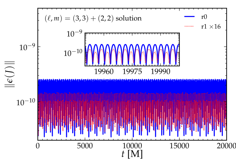
Figure 1: $L_{2}$ norm Eq. (68) of the error in the evolution variable $J$ of a superposed $(\ell,m)=(2,2)+(3,3)$ linearized solution on two resolutions $r0$ and $r1$ (Table 1). Given that the amplitude of $J$ itself is on the order of $10^{-6}$ (compare Eq. (66)), we observe that the relative error at the given resolutions is $<10^{-4}$. The error in the high resolution $r1$ is scaled for 4th-order convergence. We observe better than 4th-order convergence (see text for a discussion). The evolution is still stable after $T=20000M$. This corresponds to $\sim 6400$ cycles in the solution. The inset shows a close up of the error for the last $50M$ of evolution.

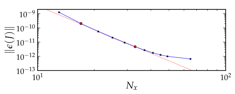
Figure 2: $L_{2}$-norm over time Eq. (71) of the error in the evolution variable $\epsilon(J)$ of a superposed $(\ell,m)=(2,2)+(3,3)$ linearized solution on multiple radial resolutions. As the radial resolution is increased starting from $N_{x}=13$ up to $N_{x}=65$ points, the error decreases at better than 4th-order. The two highlighted (red) markers correspond to resolutions $r0$ and $r1$ (Table 1), respectively. The red dashed line corresponds to a fit excluding the first point and the last four points. We measure a convergence order of $\sim 5$. When the error reaches roughly the square of the amplitude of the linearized solution ($\sim 10^{-12}$) where quadratic (and higher order) terms become important, the convergence order starts to deteriorate. This is expected since the linearized solutions only satisfy the Einstein equations to linear order.

5.2 Pseudo random noise

A strong test for stability involves injecting (pseudo) random noise into the evolution, via the initial and boundary data [35, 36]. By this method, any exponentially growing error modes, if present, will be stimulated at a much higher amplitude than would naturally occur due to truncation or round-off error.

In this test, we add noise to all spectral coefficients of $J$ on the initial null hypersurface, and also to all spectral coefficients of all remaining quantities that are needed at the inner boundary, the worldtube $\Gamma$, at each timestep. We add noise of amplitude $A_{\rm noise}=10^{-2}$ to a $(\ell,m)=(3,3)$ linearized solution with parameters given by Eq. (66). Note that the amplitude of the noise is $10,000$ times stronger than the amplitude of the linearized solution itself, and thus of nonlinear scale.

In Fig. 3, we show the norm Eq. (68) of the error $\epsilon(J)$ over a period of $T=2500M$, where we have chosen resolution $r1$ as listed in Table 1. To allow for higher frequency angular modes, in the solution we use spectral coefficients up to $\ell=8$, and increase the number of collocation points to $(N_{\theta},N_{\phi})=(18,18)$ accordingly. We inject noise not only into the $(\ell,m)=(3,3)$ solution mode, but also into all other modes up to $\ell=8$, which would otherwise be zero. To control the stability of the scheme, we set the amount of dissipation to $\epsilon_{\rm diss}=0.5$. The test demonstrates that the non-linear coupling of angular modes does not lead to unstable behavior over the observed timescale.

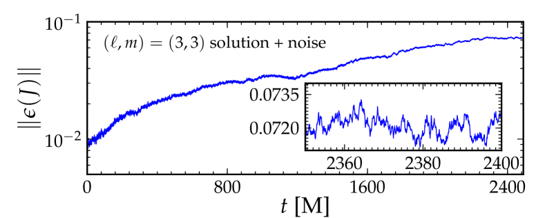
Figure 3: $L_{2}$ norm Eq. (68) of the error in the evolution variable $J$ of a $(\ell,m)=(3,3)$ linearized solution with pseudo random noise of amplitude $A_{\rm noise}=10^{-2}$ injected into modes $\ell\leq 8$ at the worldtube. The error remains bounded after a few tens of thousand iterations. This indicates that the scheme is stable even in the presence of strong noise. The inset shows a close-up of the error over a timescale of $50M$.

6 Discussion

We have developed and implemented a high-order algorithm for numerically integrating the full non-linear Einstein equations along characteristic null hypersurfaces in the Bondi-Sachs framework. The implemented code evolves the full Einstein equations in the wave zone of a compact body, remaining stable, convergent, and achieving high accuracy with relatively low computational cost compared to the previous 2nd-order algorithm. Radial integration is performed in terms of a modified Adams-Moulton scheme that is 4th-order accurate. Radial derivatives are computed in terms of 4th-order finite differences. Angular derivatives are computed in terms of spectral expansions of real-valued spin-weighted spherical harmonics. It is in principle straightforward to design an algorithm along the lines used here at even higher order of convergence than 4th-order. However, the stability properties of the algorithm are clearly dependent on its order, and achieving stability for an algorithm of higher order may be problematic.

The implemented algorithm is a first step towards more efficient gravitational-wave extraction algorithms via Cauchy-characteristic extraction. It is also a first step towards Cauchy-characteristic matching in which the characteristic evolution is used to provide on-the-fly boundary data for a 3+1 evolution. In view of this, we have designed our code such that it can run concurrently with our 3+1 evolution code. The next step will be the implementation of an improved algorithm for worldtube boundary data transformation that couple Cauchy and characteristic evolutions, and that is of higher than 2nd-order.

Appendix A The nonlinear terms in the Einstein equations

The nonlinear terms $N_{\beta},N_{Q},N_{U},N_{W}$ and $N_{J}$ in Eq. (19a) through Eq. (21) were first presented in [12]. We repeat them here, but with a mis-print in Eq. (A3) of [12] corrected.

$$N_{\beta}=\frac{r}{8}\left(J_{,r}\bar{J}_{,r}-K^{2}_{,r}\right).$$ (72)

$$N_{U}=\frac{e^{2\beta}}{r^{2}}\left(KQ-Q-J\bar{Q}\right),$$ (73)

$$N_{Q} = r^{2}\Bigg{(}(1-K)(\eth K_{,r}+\bar{\eth}J_{,r})+\eth(\bar{J}J_{,r})+\bar{\eth}(JK_{,r})-J_{,r}\bar{\eth}K$$ (74)

$$+ \frac{1}{2K^{2}}(\eth\bar{J}(J_{,r}-J^{2}\bar{J}_{,r})+\eth J(\bar{J}_{,r}-\bar{J}^{2}J_{,r}))\Bigg{)}.$$

$$N_{W} = e^{2\beta}\Bigg{(}(1-K)(\eth\bar{\eth}\beta+\eth\beta\bar{\eth}\beta)+\frac{1}{2}\bigg{(}J(\bar{\eth}\beta)^{2}+\bar{J}(\eth\beta)^{2}\bigg{)}$$ (75)

$$-\frac{1}{2}\bigg{(}\eth\beta(\bar{\eth}K-\eth\bar{J})+\bar{\eth}\beta(\eth K-\bar{\eth}J)\bigg{)}+\frac{1}{2}\bigg{(}J\bar{\eth}^{2}\beta+\bar{J}\eth^{2}\beta\bigg{)}\Bigg{)}$$

$$-e^{-2\beta}\frac{r^{4}}{8}(2KU_{,r}\bar{U}_{,r}+J\bar{U}^{2}_{,r}+\bar{J}U^{2}_{,r}).$$

$$N_{J}=N_{J1}+N_{J2}+N_{J3}+N_{J4}+N_{J5}+N_{J6}+N_{J7}+\frac{J}{r}(P_{1}+P_{2}+P_{3}+P_{4})$$ (76)

where

$$N_{J1} = -\frac{e^{2\beta}}{r}\bigg{(}K(\eth J\bar{\eth}\beta+2\eth K\eth\beta-\bar{\eth}J\eth\beta)+J(\bar{\eth}J\bar{\eth}\beta-2\eth K\bar{\eth}\beta)-\bar{J}\eth J\eth\beta\bigg{)},$$

$$N_{J2} = -\frac{1}{2}\bigg{(}\eth J(r\bar{U}_{,r}+2\bar{U})+\bar{\eth}J(rU_{,r}+2U)\bigg{)},$$

$$N_{J3} = (1-K)(r\eth U_{,r}+2\eth U)-J(r\eth\bar{U}_{,r}+2\eth\bar{U}),$$

$$N_{J4} = \frac{r^{3}}{2}e^{-2\beta}\bigg{(}K^{2}U^{2}_{,r}+2JKU_{,r}\bar{U}_{,r}+J^{2}\bar{U}^{2}_{,r}\bigg{)},$$

$$N_{J5} = -\frac{r}{2}J_{,r}(\eth\bar{U}+\bar{\eth}U),$$

$$N_{J6} = r\Bigg{(}\frac{1}{2}(\bar{U}\eth J+U\bar{\eth}J)(J\bar{J}_{,r}-\bar{J}J_{,r})$$

$$+(JK_{,r}-KJ_{,r})\bar{U}\bar{\eth}J-\bar{U}(\eth J_{,r}-2K\eth KJ_{,r}+2J\eth KK_{,r})$$

$$-U(\bar{\eth}J_{,r}-K\eth\bar{J}J_{,r}+J\eth\bar{J}K_{,r})\Bigg{)},$$

$$N_{J7} = r(J_{,r}K-JK_{,r})\bigg{(}\bar{U}(\bar{\eth}J-\eth K)+U(\bar{\eth}K-\eth\bar{J})$$

$$+K(\bar{\eth}U-\eth\bar{U})+(J\bar{\eth}\bar{U}-\bar{J}\eth U)\bigg{)},$$

$$P_{1} = r^{2}\bigg{(}\frac{J_{,u}}{K}(\bar{J}_{,r}K-\bar{J}K_{,r})+\frac{\bar{J}_{,u}}{K}(J_{,r}K-JK_{,r})\bigg{)}-8\left(r+r^{2}\hat{W}\right)\beta_{,r},$$

$$P_{2} = e^{2\beta}\Bigg{(}-2K(\eth\bar{\eth}\beta+\bar{\eth}\beta\eth\beta)-(\bar{\eth}\beta\eth K+\eth\beta\bar{\eth}K)$$

$$+ \bigg{(}J(\bar{\eth}^{2}\beta+(\bar{\eth}\beta)^{2})+\bar{J}(\eth^{2}\beta+(\eth\beta)^{2})\bigg{)}+(\bar{\eth}J\bar{\eth}\beta+\eth\bar{J}\eth\beta)\Bigg{)},$$

$$P_{3} = \frac{r}{2}\bigg{(}(r\bar{\eth}U_{,r}+2\bar{\eth}U)+(r\eth\bar{U}_{,r}+2\eth\bar{U})\bigg{)},$$

$$P_{4} = -\frac{r^{4}}{4}e^{-2\beta}(2KU_{,r}\bar{U}_{,r}+J\bar{U}^{2}_{,r}+\bar{J}U^{2}_{,r}).$$ (77)

Appendix B Regularized equations at $\mathcal{J}^{+}$

At $\mathcal{J}^{+}$, the equations simplify when inserting Eq. (25) and Eq. (26) and taking the limit $r\rightarrow\infty$. In particular, terms containing powers of $1/r,...,1/r^{n}$ vanish. Below, we give the equations evaluated at $\mathcal{J}^{+}$.

$$\beta_{,x} = 0\,,$$ (78)

$$Q = -2\eth\beta\,,$$ (79)

$$U_{,x} = r_{\Gamma}^{-1}e^{2\beta}(KQ-J\bar{Q})\,,$$ (80)

$$\hat{W} = \frac{\eth\bar{U}+\bar{\eth}U}{2}\,,$$ (81)

$$\Phi = -\eth U+N_{J,\mathcal{J}^{+}}\,,$$ (82)

where

$$N_{J,\mathcal{J}^{+}}=-\frac{\bar{U}\eth J+U\bar{\eth}J}{2}+(1-K)\eth U-\frac{J(\eth\bar{U}-\bar{\eth}U)}{2}\,.$$ (83)

Appendix C Dissipation operator stencil

Close to the outer boundary where we do not have enough points to apply the standard centred-stencil Kreiss-Oliger dissipation operator Eq. (50), we use side-winded dissipation operator stencils derived for SBP operator $D_{4-2}$ of [25]. This particular dissipation operator is defined via coefficients $a_{ij}$ and $q_{i}$. In the interior of the domain the operator reads

$$A_{ij}u_{j} = \frac{\epsilon_{\rm diss}}{2^{2p}}\left[q_{0}u_{i}+\sum_{j=1}^{7}q_{j}\left(u_{i-j}+u_{i+j}\right)\right]$$ (84)

where the $q_{i}$ are the coefficients given in Eq. (50). Near the outer boundary (on points $i=N_{x}-5,...,N_{x}-1$), the operator can be written as

$$A_{ij}u_{j} = \frac{\epsilon_{\rm diss}}{2^{2p}}\sum_{j=1}^{7}a_{j,N_{x}-i}u_{N_{x}-j},$$ (85)

where the coefficients $a_{ij}$ are taken from [25] reported below. We note that $\epsilon_{\rm diss}\geq 0$ selects the amount of dissipation and is usually of order unity.

$$(a_{ij})=\left(\begin{array}[]{ccccccc}-\frac{48}{17}&\frac{144}{17}&-\frac{144}{17}&\frac{48}{17}&0&0&0\\ \frac{144}{59}&-\frac{480}{59}&\frac{576}{59}&-\frac{288}{59}&\frac{48}{59}&0&0\\ \frac{144}{43}&\frac{576}{43}&-\frac{912}{43}&\frac{720}{43}&-\frac{288}{43}&\frac{48}{43}&0\\ \frac{48}{49}&-\frac{288}{49}&\frac{720}{49}&-\frac{960}{49}&\frac{720}{49}&-\frac{288}{49}&\frac{48}{49}\end{array}\right)$$ (86)

References

References

- [1] C. Reisswig, N. T. Bishop, D. Pollney, and B. Szilagyi. Unambiguous determination of gravitational waveforms from binary black hole mergers. Phys. Rev. Lett., 103:221101, 2009.
- [2] C. Reisswig, N. T. Bishop, D. Pollney, and B. Szilagyi. Characteristic extraction in numerical relativity: binary black hole merger waveforms at null infinity. Class. Quant. Grav., 27:075014, 2010.
- [3] M.C. Babiuc, B. Szilagyi, J. Winicour, and Y. Zlochower. A Characteristic Extraction Tool for Gravitational Waveforms. Phys.Rev., D84:044057, 2011.
- [4] M.C. Babiuc, J. Winicour, and Y. Zlochower. Binary Black Hole Waveform Extraction at Null Infinity. Class.Quant.Grav., 28:134006, 2011.
- [5] C. Reisswig, C.D. Ott, U. Sperhake, and E. Schnetter. Gravitational Wave Extraction in Simulations of Rotating Stellar Core Collapse. Phys.Rev., D83:064008, 2011.
- [6] C. D. Ott, C. Reisswig, E. Schnetter, E. O’Connor, U. Sperhake, F. Löffler, P. Diener, E. Abdikamalov, I. Hawke, and A. Burrows. Dynamics and Gravitational Wave Signature of Collapsar Formation. Phys. Rev. Lett., 106:161103, April 2011.
- [7] Jeffrey Winicour. Characteristic evolution and matching. Living Rev. Relativ., 8:10, 2005. [Online article].
- [8] H. Bondi, M. G. J. van der Burg, and A. W. K. Metzner. Gravitational waves in general relativity VII. Waves from axi-symmetric isolated systems. Proc. Roy. Soc. A, 269:21–52, 1962.
- [9] R. K. Sachs. Gravitational waves in general relativity. Proc. Roy. Soc. A, 270:103–126, 1962.
- [10] R. Penrose. Asymptotic properties of fields and spacetimes. Phys. Rev. Lett., 10:66–68, 1963.
- [11] N. T. Bishop, R. Gómez, L. Lehner, and J. Winicour. Cauchy-characteristic extraction in numerical relativity. Phys. Rev. D, 54:6153–6165, 1996.
- [12] Nigel T. Bishop, Roberto Gómez, Luis Lehner, Manoj Maharaj, and Jeffrey Winicour. High-powered gravitational news. Phys. Rev. D, 56(10):6298–6309, 15 November 1997.
- [13] F. Löffler, J. Faber, E. Bentivegna, T. Bode, P. Diener, R. Haas, I. Hinder, B. C. Mundim, C. D. Ott, E. Schnetter, G. Allen, M. Campanelli, and P. Laguna. The Einstein Toolkit: a community computational infrastructure for relativistic astrophysics. Classical and Quantum Gravity, 29(11):115001, 2012.
- [14] Roberto Gómez, Jeffrey Winicour, and Richard Isaacson. Evolution of scalar fields from characteristic data. J. Comput. Phys., 98:11 – 25, 1992.
- [15] Christian Reisswig, Nigel T. Bishop, Chi Wai Lai, Jonathan Thornburg, and Belá Szilágyi. Characteristic evolutions in numerical relativity using six angular patches. Class. Quantum Grav., 24:S327–S339, 2007.
- [16] Roberto Gomez, Willians Barreto, and Simonetta Frittelli. A framework for large-scale relativistic simulations in the characteristic approach. Phys. Rev., D76:124029, 2007.
- [17] Robert Bartnik. Einstein equations in the null quasispherical gauge. Class.Quant.Grav., 14:2185–2194, 1997.
- [18] Robert A. Bartnik and Andrew H. Norton. Einstein equations in the null quasi-spherical gauge III: numerical algorithms. gr-qc/9904045, 1999.
- [19] Nigel T. Bishop, C. Clarke, and R. d’Inverno. Numerical relativity on a transputer array. Class. Quantum Grav., 7(2):L23–L27, February 1990.
- [20] J. M. Stewart. Advanced general relativity. Cambridge University Press, Cambridge, 1990.
- [21] Roberto Gómez, Luis Lehner, Philippos Papadopoulos, and Jeffrey Winicour. The eth formalism in numerical relativity. Class. Quantum Grav., 14(4):977–990, 1997.
- [22] J. N. Goldberg, A. J. MacFarlane, Ezra T. Newman, F. Rohrlich, and E. C. G. Sudarshan. Spin- spherical harmonics and . J. Math. Phys., 8(11):2155–2161, 1967.
- [23] W. H. Press, S. A. Teukolsky, W. T. Vetterling, and B. P. Flannery. Numerical recipes in C++ : the art of scientific computing. New York, 3rd edition, 2002.
- [24] James R. Driscoll and Dennis M. Healy, Jr. Computing fourier transforms and convolutions on the 2-sphere. Adv. Appl. Math., 15(2):202–250, 1994.
- [25] Peter Diener, Ernst Nils Dorband, Erik Schnetter, and Manuel Tiglio. Optimized high-order derivative and dissipation operators satisfying summation by parts, and applications in three-dimensional multi-block evolutions. J. Sci. Comput., 32:109–145, 2007.
- [26] T. Goodale, G. Allen, G. Lanfermann, J. Massó, T. Radke, E. Seidel, and J. Shalf. The Cactus framework and toolkit: Design and applications. In Vector and Parallel Processing – VECPAR’2002, 5th International Conference, Lecture Notes in Computer Science, Berlin, 2003. Springer.
- [27] http://www.cactuscode.org.
- [28] Erik Schnetter, Scott H. Hawley, and Ian Hawke. Evolutions in 3D numerical relativity using fixed mesh refinement. Class. Quantum Grav., 21(6):1465–1488, 21 March 2004.
- [29] http://www.carpetcode.org.
- [30] Christian Reisswig. Binary Black Hole Mergers and Novel Approaches to Gravitational Wave Extraction in Numerical Relativity. PhD thesis, Leibniz Universität Hannover, 2010.
- [31] Denis Pollney, Christian Reisswig, Erik Schnetter, Nils Dorband, and Peter Diener. High accuracy binary black hole simulations with an extended wave zone. arXiv:0910.3803, 2009.
- [32] Denis Pollney, Christian Reisswig, Nils Dorband, Erik Schnetter, and Peter Diener. The Asymptotic Falloff of Local Waveform Measurements in Numerical Relativity. Phys. Rev., D80:121502, 2009.
- [33] Nigel T. Bishop, Roberto Gómez, Paulo R. Holvorcem, Richard A. Matzner, Philippos Papadopoulos, and Jeffrey Winicour. Cauchy-characteristic matching: A new approach to radiation boundary conditions. Phys. Rev. Lett., 76(23):4303–4306, 3 June 1996.
- [34] Nigel T. Bishop. Linearized solutions of the Einstein equations within a Bondi-Sachs framework, and implications for boundary conditions in numerical simulations. Class. Quantum Grav., 22(12):2393–2406, 2005.
- [35] B. Szilágyi, Roberto Gomez, N. T. Bishop, and Jeffrey Winicour. Cauchy boundaries in linearized gravitational theory. Phys. Rev. D, 62:104006, 2000.
- [36] Miguel Alcubierre, Gabrielle Allen, Thomas W. Baumgarte, Carles Bona, David Fiske, Tom Goodale, Francisco Siddhartha Guzmán, Ian Hawke, Scott Hawley, Sascha Husa, Michael Koppitz, Christiane Lechner, Lee Lindblom, Denis Pollney, David Rideout, Marcelo Salgado, Erik Schnetter, Edward Seidel, Hisa aki Shinkai, Deirdre Shoemaker, Béla Szilágyi, Ryoji Takahashi, and Jeffrey Winicour. Towards standard testbeds for numerical relativity. Class. Quantum Grav., 21(2):589–613, 2004.