Coordination Level Modeling and Analysis of Parallel Programs using Petri Nets

Abstract

In the last fifteen years, the high performance computing (HPC) community has claimed for parallel programming environments that reconciles generality, higher level of abstraction, portability, and efficiency for distributed-memory parallel computing platforms. The Hash component model appears as an alternative for addressing HPC community claims for fitting these requirements. This paper presents foundations that will enable a parallel programming environment based on the Hash model to address the problems of “debugging”, performance evaluation and verification of formal properties of parallel program by means of a powerful, simple, and widely adopted formalism: Petri nets.

1 Introduction

Haskell$\#$ is a parallel extension to Haskell [6], the most widely used non-strict pure functional programming language [25]. It makes possible the coordination of a set of functional processes written in Haskell through a configuration language, called HCL (Haskell$\#$ Configuration Language). Thus, Haskell_# separate the programming task in two levels: the computation level, where functional processes are written in Haskell, and the coordination level, where functional processes are coordinated. The coordination media of Haskell_# is also called the Hash component model. In recent works, we have generalized the Hash component model in order to support other programming languages than Haskell at the computation level. Functional processes are now units, possibly written in any programming language supported by a programming environment that complies to the Hash component model. In this paper, we still suppose that units are the functional processes of Haskell$\#$.

The coordination level of Haskell_#, i. e. the Hash component model, was designed in order to make possible to translate the coordination media of Haskell$\#$ programs onto Petri nets. This paper addresses the issue of presenting a translation schema for that, demonstrating its use to formal analysis of them, involving verification of formal properties. The use of Petri nets allows for reusing existing automatic tools based on this formalisms for reasoning about Hash programs, such as PEP [4] and INA [21]. Further extensions could make possible performance evaluation using timed or stochastic Petri Nets variants [14, 26].

In the rest of the paper, we use the Hash component model to refer to the coordination level of Haskell_#, i.e. it is assumed that functional processes are written in Haskell (functional modules) and they communicate through either stream-based or singleton communication channels that link their input and output ports. Such concepts are not present in the general definition of the Hash component model.

In additional to this introduction, this paper comprises the following sections. Section 2 presents additional details about the Hash component model. Section 3 presents a translation schema of Hash programs onto Petri nets. Section 4 demonstrates how Petri net models of Hash programs may be used for verification of formal concurrency properties of Hash programs.

2 The Hash Component Model

Distributed parallel programs may be viewed as collections of processes that interact by exchanging messages during execution. Current programming models provide the ability to describe computation of processes by augmenting common languages with notations for explicit message passing. However, they do not provide ability to modularize concerns that appear in the design of parallel applications, including the concern of parallelism itself, which are scattered across the implementation of processes. We advocate that this is the key feature for integrating advanced software engineering techniques in the development environment of HPC parallel applications. In sequential programming, the focus is on modularization of concerns, since there are a unique conceptual “process” and efficiency requirements are less restrictive. This is the essential difference that makes sequential programming actually more suitable for current software engineering techniques for large scale applications than current parallel programming.

The Hash component model may be viewed as a new paradigm for developing message passing programs. Now, they may be viewed from two orthogonal perspective dimensions: the dimension of processes and the dimension of components.

A process correspond to the related notion derived from conventional message passing programming. Thus, they are agents that perform computational tasks, communicating through communication channels. Conceptually, Hash channels, like in OCCAM [17], are point-to-point, synchronous, typed and unidirectional. Bounded buffers are also supported. The disciplined use of channels is the feature that makes possible formal analysis of parallel programs by using Petri nets, the main topic of this paper.

A component is an abstract entity that address a functional or non-functional concern of the application or its execution environment in the parallel program. A component describe the role of a set of processes with respect to a given concern. The sets of components that respectively implement a set of concerns may overlap, allowing for modular separation of concerns that are interlaced across implementation of processes (cross-cutting concerns). The separation of cross-cutting concerns is an active research area in object-oriented programming of large scale applications [19]. A Hash program is defined by a main component that address the overall application concern. Some common examples of cross-cutting non-functional concerns that appears in HPC applications are: placement of processes onto processors, secure policies for accessing computing resources on grids, fault-tolerance schemes for long-running applications, parallel debugging, execution timing, and so on.

Hash programming is performed from the perspective of components, instead of processes, but resulting in the specification of the topology of a network of parallel processes.

Components may be composed or simple. Composed components are programmed using the Hash configuration language (HCL), being built by hierarchical composition of other components, called inner components. HCL may be viewed as a language for gluing and orchestrating components, i.e. a connector language. It is distinguished from other compositional languages because it supports composition of parallel components by overlapping the concerns they address. Conventional compositional languages only allows nested composition of sequential components. Simple components addresses functional concerns, implemented using a host language, supposed to be sequential. Simple components are the atoms of functionality in Hash programs, constituting the leaves in their component hierarchy.

The Hash component model supports parallel programming with skeletons [11] without any additional language support. Partial topological skeletons may expose topological patterns of interaction between processes in a Hash program, which may be used to produce more efficient code for specific architectures and execution environments [8]. They are implemented as composed components parameterized by their addressed concerns.

The Hash component model has origins in Haskell_# [6], where the host language used to program simple components is Haskell. Haskell enables separation between coordination and computation code, by attaching lazy streams to communication channels at coordination level, avoiding the use of communication primitives in communication code [5]. This paper on focused in Haskell_#.

In the next section, it is described how composed components, and skeletons, are programmed using Hash configurations, while programming of simple components, in Haskell, is described in Section 2.2.

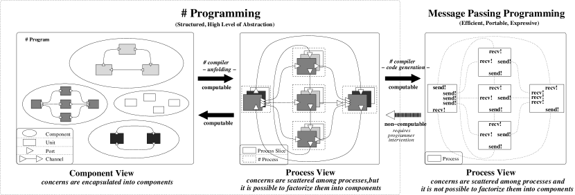
Figure 1: Component Perspective versus Process Perspective

2.1 Programming Composed Components

Composed components define coordination media of Haskell_# programs, where all parallelism concerns are addresses without mention to entities at computation levels, where computations are specified. Composed components are written in HCL (Hash Configuration Language). Also, they define the core of the Hash component model, supported by Haskell_#.

Figure 2: Instantiating and Configuring a Unit

The configuration of a composed component specifies how a collection units, agents that perform specific tasks, interact by means of point-to-point, typed, and unidirectional communication channels, for addressing a given parallel programming concern. For that, a unit is instantiated from an interface and associated to a component (Figure 2). The latter specifies the task performed by the unit, since functional modules describe addressed concerns, while the former specifies how the unit interacts with the coordination medium. A unit associated with a simple component is called process, while a unit associated with a composed component is called a cluster. A interface of a unit is defined by a set of typed input and output ports and a protocol. The protocol of an interface specifies the order in which ports may be activated during execution of the units instantiated from that interface, by means of an embedded language whose constructors have semantic equivalence to regular expressions controlled by semaphores. This formalism is equivalent to place/transition Petri nets, allowing for formal property analysis, simulation and performance evaluation of programs using available Petri net tools [10], such as PEP [16] and INA [21]. A port is activated between the time in which it becomes ready to perform a communication operation and the time it completes this operation, according to the communication mode of the channel where the port is connected.

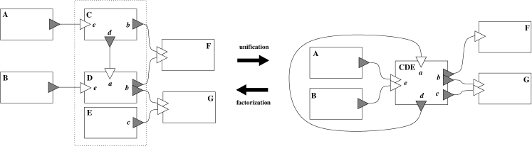
Figure 3: Unification/Factorization

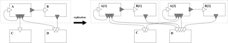
Figure 4: An Illustrative Example of Replication

Units interact through communication channels, which connect an output port from an unit (transmitter) to an input port of another one (receiver). The types of the connected ports must be the same. The supported communication modes, inspired on MPI, are : synchronous, buffered and ready.

In a unit specification, interface ports can be replicated to form groups. Groups may be of two kinds: any and all, according to the semantics of activation. The activation of a group of ports of kind all implies activation of all its port members. The activation of a group of ports of kind any implies that one of the port members will be put ready for communication but only one will complete communication. The chosen port is one of the activated ports whose communication pairs are also activated at that instant. From the internal perspective of the unit, groups are treated as indivisible entities, while from the perspective of the coordination medium, port members are referred directly in order to forming channels. Input and output ports (groups individually) of the unit interface must be mapped to arguments and return points of the component assigned to it, respectively. Wire functions are useful when it is necessary to transform values at the boundary between ports and arguments/exit points. A particularly useful use of wire functions is to aggregate data received from input ports belonging to a group of ports of kind all to a unique value, passed to the associated argument. Similarly, wire functions allow that a value produced in an exit point to be mapped onto a collection of values in order to be sent by the port members of the associated group of output ports of kind all. Wire functions increases the changes for reusing a component, resolving possible conflicts.

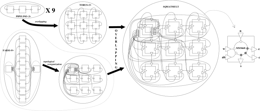
Figure 5: Topology of Matrix Multiplication Using a Torus

Two operations are defined on units: unification and factorization. Unification allows to unify a collection of units, forming a single unit. Factorization is the inverse of unification, allowing units to be divided into many virtual units. Replication, a third operation applied to units, allows that the network induced by a collection of units to be replicated. All operations assume that units are fully connected. Behavioral and connectivity preserving restrictions are applied, but not formalized here. Connectivity restrictions imply the possibility of to replicate ports whenever it is necessary to adjust topological connectivity after an operation. Figures 3 and 4 present illustrative examples of these operations.

2.1.1 Virtual Units and Skeletons

To allow overlapping of components and the support for skeletons, the notion of virtual unit has been introduced. A unit is virtual whenever there is no component associated with it. In other terms, the task performed by a virtual unit is not defined. Components are partially parameterized in its addressed concern by means of placing virtual units in its constitution. A component that comprises at least one virtual unit is called an abstract component, or a partial topological skeleton. These terms are used as synonyms. When a programmer re-use an abstract component for specification of a Hash program, it must to assign components to the virtual units comprising it.

Abstract components may not instantiate applications. It is necessary to describe the computation performed by their constituent virtual units. The assignment operation is used allows to associate a component to a virtual unit, making it a non-virtual unit. Also, there is a superseding operation, which allows to take a non-virtual unit for replacing a virtual unit of the topology. The behavioural compatibility restrictions from the non-virtual unit to the replaced virtual unit guarantees that any sequence of communication actions that is valid in the non-virtual unit remains valid in the virtual unit. The superseding operation is a “syntactic sugar” of HCL, since it may be implemented using unification and assignment.

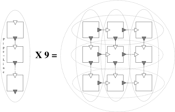
Figure 6: Composing Pipe-Lines to Form a Systolic Mesh

Figure 6 shows how a skeleton describing a systolic mesh of processes, implemented by overlapping a collection of pipe-line skeleton instances. The abstract components PipeLine is used to describe interaction of processes placed at the mesh lines and columns. Each unit in SystolicMesh abstract component is formed by two slices: one described by the unit that comes from the vertical PipeLine component and the other described by the unit that comes from the horizontal one.

component CPipeLine $<$N$>$ with iterator i range [1,N] interface ICPipe where ports: i* $\rightarrow$ o* protocol: repeat seq{o!; i?} until $<$o & i$>$ $[/$ unit pipe[i] where ports: ICPipe $/]$ connect pipe[i]$\rightarrow$o to pipe[i+1]$\leftarrow$i, buffered component Torus $<$N$>$ with use Skeletons.Common.CPipeLine iterator i, j range [1,N] interface ITorus where ports: ICPipe @ n $\rightarrow$ s # ICPipe @ e $\rightarrow$ w protocol: repeat seq { par {s!; w!}; par {n?; e?}} until $<$n & e & s & w$>$ $[/$ unit vpipe[i]; assign CPipeLine$<$N$>$ to vpipe[i] $/]$ $[/$ unit hpipe[j]; assign CPipeLine$<$N$>$ to hpipe[j] $/]$ $[/$ unify vpipe[i].pipe[j], hpile[j].pipe[i] to node[i][j] where ports: ITorus $/]$ component Farm$<$N$>$ with unit distributor where ports: () $\rightarrow$ job unit worker where ports: job $\rightarrow$ result protocol: seq {job?; result!} unit collector where ports: result $\rightarrow$ () connect distributor.job to worker.job, synchronous connect worker.result to collector.result, synchronous replicate N: worker

component SqMatMult$<$N$>$ where iterator $i$, $j$ range [1,N] use Skeletons.Common.{Torus, Farm} use MMShift int erface ISqMatMult where ports: j $\rightarrow$ r # ITorus protocol: seq {j?; repeat seq {s!;e!;n?;w?} counter $N$ } unit mm_torus; assign Torus$<$N$>$ to mm_torus unit mm_farm; assign Farm$<$N$>$ to mm_farm $[/$ unify farm.worker[$i+j\times N$], torus.node[$i$][$j$] to sqmm[$i$][$j$] $/]$ where ports: ISqMatMult unify farm.distributor, farm.collector, sqmm[0][0] to sqmm_root where ports: () $\rightarrow$ ab # c $\rightarrow$ () # ISqMatMult @ mm protocol: seq {ab!; c?; do mm } $[/$ assign MMShift to sqmm[$i$][$j$] $/]$ module MMShift(main) where main :: Num t $\Rightarrow$ t $\rightarrow$ t $\rightarrow$ [t] $\rightarrow$ [t] $\rightarrow$ ([t],[t],t) main a b as_i bs_i = (as_o,bs_o,c) where c = matmult as_o bs_o (as_o, bs_o) = (a:as_i, b:bs_i) matmult :: Num t $\Rightarrow$ t $\rightarrow$ [t] $\rightarrow$ [t] $\rightarrow$ t matmult [] [] = 0 matmult (a:as) (b:bs) = a*b + matmult as bs

Figure 7: Configuration Code of Matrix Multiplication on a Torus

module Tracking(main) where
import Track
import Tallies
import Mcp_types
main :: User_spec_info $\rightarrow$ [(Particle,Seed)] $\rightarrow$ ([[Event]],[Int])
main	user_info particle_list =	let	events’s = map f particle_list in (events’s, tally_bal event_lists)
	where
		f (particle@(_,_,_, e, _), sd) = (Create_source e):(track user_info particle [] sd)

Figure 8: A Functional Module from MCP-Haskell_#

2.2 Programming Simple Components

Simple components, also called functional modules, are atoms of functionalities in Hash programming. The collection of simple components in a Hash program describes its computation media. Simple components might be programmed virtually in any general purpose language, called host language. For that, it is needed to define which host language constructions correspond to the arguments and return points of the underlying functional module. It is preferred that no extensions to the host language be necessary for this purpose, keeping transparency between coordination and computation media. Simple components may be overlapped when configuring composed components. The goal is to implement a really multi-lingual approach for parallel programming. For that, it has been proposed to use CCA (Common Component Architecture) [2], a recent standard proposed for integrating components written in different languages in a parallel environment. Another possibility is to use heterogeneous implementations of MPI [24, 23], recently proposed, facilitating this task since, in cluster environments, Hash programs are compiled to MPI.

Since the translation schema onto Petri nets is defined on top of coordination media, abstracting from computation media concerns, specific details about programming simple components is not provided in this paper. For illustration, Figure 8 presents an example of functional module from MCP-Haskell_# program [9], written in Haskell.

$<$Component$>$ $\rightarrow$ component (	{$u_{1}$:$<$Unit$>$, $\dots$, $u_{i}$:$<$unit$>$}, {$c_{1}$:$<$Channel$>$, $\dots$,$c_{j}$:$<$Channel$>$})
$<$Unit$>$ $\rightarrow$ unit ($id$, {$p_{1}$:$<$Port$>$, $\dots$, $p_{k}$:$<$Port$>$}, $<$Typeu$>$)
$<$Typeu$>$ $\rightarrow$ repetitive $\mid$ non-repetitive
$<$Behavior$>$ $\rightarrow$ protocol ($\{id^{sem}_{1},\dots,id^{sem}_{n}\}$, $<$Action$>$)
$<$Action$>$	$\rightarrow$	skip
	$\mid$	seq {$a_{1}$:$<$Action$>$; $\dots$; $a_{k}$:$<$Action$>$}
	$\mid$	par {$a_{1}$:$<$Action$>$; $\dots$; $a_{k}$:$<$Action$>$}
	$\mid$	alt {$g_{1}$:$<$Action$>$; $\dots$; $g_{k}$:$<$Action$>$}
	$\mid$	repeat_until ($<$Action$>$, C)
	$\mid$	repeat_counter ($<$Action$>$, N)
	$\mid$	repeat_forever $<$Action$>$
	$\mid$	signal $id$
	$\mid$	wait $id$
	$\mid$	activate $id$
$<$Port$>$ $\rightarrow$ port ($id$,$<$Direction$>$,$<$Multiplicity$>$,$<$Typep$>$,$nesting\_factor$)
$<$Multiplicity$>$	$\rightarrow$	single $\mid$ group ($<$Typeg$>$, {$p_{1}$:$<$Port$>$, $\dots$, $p_{n}$:$<$Port$>$})
$<$Direction$>$ $\rightarrow$ input $\mid$ output
$<$Typep$>$ $\rightarrow$ stream $\mid$ non-stream
$<$Typeg$>$ $\rightarrow$ any $\mid$ all
$<$Channel$>$ $\rightarrow$ connect ($id^{port}$, $id^{port}$, $<$ChanMode$>$)
$<$ChanMode$>$ $\rightarrow$ synchronous $\mid$ buffered $\mid$ ready

Figure 9: Abstract Hash Configuration Language Syntax

2.3 An Abstract Representation for Hash Components

In Figure 9, it is defined a simplified syntax for an abstract representation of Hash configurations, named Abstract Hash. The abstract Hash configuration language (AHCL) only captures information strictly relevant to the translation schema onto Petri nets further presented. For example, interface declarations and operations over units, such as unifications, factorizations, replications, and assign operation are not represented in AHCL. It is supposed that these operations are all resolved before translation process. AHCL is not a simplification. Indeed, in the compilation process of Hash configurations, AHCL correspond to the intermediate code generated by the front-end compiler module, which serves as input to all back-end modules. A back-end was developed for generating PNML (Petri Net Markup Language) code from a Hash configuration. The following paragraph describes the structure of AHCL.

A component is composed by a set of units ($u_{1},\dots,u_{i}$) and a set of channels ($c_{1},\dots,c_{j}$). Units are described by an identifier, a collection of ports ($<\textsc{Port}>$). A unit can be repetitive or non-repetitive ($<\textsc{Type${}_{u}$}>$). The interface of a unit is defined by a collection of ports and a protocol, described by means of an embedded language that specifies valid orders for activation of ports. This language have constructors equivalent to combinators of regular expressions controlled by balanced semaphores. A port is described by an identifier ($id$), a direction ($<\textsc{Direction}>$), a type (stream or non-stream) and a nesting factor. Additionally, port multiplicity specifies if a port is a single port or a group of ports. Notice that a group of port can be of two types: any or all. All port identifiers are assumed to be distinct in an abstract Hash programs. A channel connect two ports and is associated to a mode (synchronous, buffered and ready). Notice that, abstract Hash syntax does not force that these two ports be from opposite directions. This restriction is implicitly assumed.

Figure 10: Translating a Component

3 Translating Hash programs into Petri Nets

In this section, a schema for translating Hash programs into Petri nets is introduced. In order to make translation schema easier to understand, it is informally described using diagrams. The possibility of making intuitive visual descriptions is an interesting feature of Petri nets.

The translation schema is specified inductively in the hierarchy of components at the coordination medium of the Hash program. Thus, simple components are ignored. The overall steps in the translation procedure of a Hash program into an interlaced Petri net are:

1. Translating units: For each unit comprising the component (unit declarations), its interface is used for yielding an interlaced Petri net describing activation order of their interface ports. In Hash configuration language, it is defined by an embedded language, in interface declarations, whose combinators have correspondence to operators of regular expression controlled by semaphores. This formalism was proved to have expressiveness equivalence to Petri nets according to formal language theory. If a unit is a cluster (a composed component is assigned to the unit), it is necessary to generate the Petri net that corresponds to the assigned component. Using information about mapping of argument/return points to input/output ports of the unit, it is possible to synchronize behavior of the unit with behavior of the component, in such way that they are compatible;

2. Synchronize units. Now that a Petri net exists for describing communication behavior (traces) of each unit, communication channels (connect declarations) may be used for coordinating synchronized behavior of these Petri nets (units);

3. Synchronize streams. For each port carrying a stream, a Petri net describing a protocol for stream synchronization is overlapped with the Petri net produced in the last step. The semantics of stream communication is described separately because it increases complexity of the generated interlaced Petri net, making computationally hard its analysis. Thus, in Hash programming environment, the programmer may decide not to include stream synchronization protocol. Obviously, information may be lost, but it may not be necessary for some useful analysis.

The next sections provide details about the above translation steps. Also, it is discussed how higher-level information encompassed in skeletons may be used to simplify the generated network.

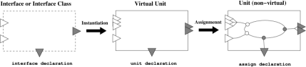
Figure 11: Unit = Interface (by instantiation) + Component (by assignment)

3.1 Modelling Components $(\Upsilon^{C})$

In Figure 10, the Petri net resulted from application of translation function $\Upsilon^{C}$ to the configuration of a component is illustrated. The translation function $\Upsilon^{U}$ is applied to each unit comprising the component, generating a Petri net that describes its communication behavior. The resulting Petri nets are connected in order to model parallel execution of units. The places process_started[$j$] and process_finished[$j$], $1\leq j\leq n$, where $n$ is the number of units, correspond to start places and stop places of the Petri nets modelling units, respectively. When a token is placed on process_started[$j$], the unit $j$ is ready to initiate execution, and when a token is placed on process_finished[$j$], the unit $j$ had finished. The transitions process_restart[$k$], $1\leq k\leq r$, where $r$ is the number of repetitive units, allows that repetitive units return back to its initial state after finalization. They are introduced in the Petri net generated for each unit. The place program_end_ready receives a mark when all non-repetitive units terminates. In this case, the tokens in places process_restart_enabled[$k$], $1\leq k\leq r$, are removed, preventing repetitive processes execute again. At this state, the program terminates after all repetitive processes also terminate, which causes transition processes_all_join to be fired and a token to be deposited in program_end.

Figure 12: Translating Unit’s Ports

3.2 Modelling Units $(\Upsilon^{U})$

This section intends to describe how individual units are translated into Petri nets. Firstly, Figure 12 presents interlaced Petri nets that model the activation of the ports of the interface of a unit. A mark in place port_prepared[$p$] indicates that the port $p$ is prepared for communication. The firing of transition port_send[$p$]/port_recv[$p$] models communication, causing the deposit of a mark in place port_complete[$p$] for indicating that communication has been completed on port $p$. It is possible that two ports be active at the same time. In groups of ports, the places group_prepare[$g$] and group_complete[$g$] are connected to places port_prepared[$p$] and port_complete[$p$] of each port $p$ belonging to the group $g$ that model local preparation and completion of communication in ports belonging to the group, according to their semantics: any or all. In groups of ports of kind all, all individual ports are activated in consequence of activation of the group. In groups of ports of kind any, only one port is chosen among the ports that are ready for communication completion. For obeying this semantic restriction, the firing of a transition port_send[$p$]/port_recv[$p$] of a port $p$ in group $g$ of kind any causes removal of the marks in places port_prepared[$p^{\prime}$], for all places $p^{\prime}$ belonging to $g$, in such a way that all ports $p$, such that $\overline{p}\neq p$, cannot complete communication (firing of transition port_send[$\overline{p}$]/port_recv[$\overline{p}$]).

The order in which marks are placed in places port_prepared[$p$], for any $p$, is controlled by an interlaced Petri net that models the protocol of the unit. The following sections discusses how primitive actions and action combinators of behavior expressions are translated into Petri nets. The primitive actions are: skip (null action), wait (increment semaphore primitive), signal (decrement semaphore primitive), ? (activation of input port), and ! (activation of output ports). The combinators of actions are: seq (sequential actions), par (concurrent actions), alt (non-deterministic choice among $n$ actions), and if (conditional choice between two actions).

Figure 13: Translating “Null Action”

3.2.1 Null Action (skip)

The skip combinator have no communication effect. Because that, it is known as the “null action”. Only one place is needed, where it is both start and stop place (Figure 13) of the interlaced Petri net generated.

3.2.2 Sequencing (seq)

Figure 14: Sequence of Actions

The seq combinator describes a total ordering for execution of a set of actions (sequential execution), represented by $a_{1},a_{2},\dots,a_{n}$. It may be modelled by sequential composition of the Petri nets induced for each action (Figure 14).

Figure 15: Interleaving (Concurrency) Among Actions

3.2.3 Concurrency (par)

The par combinator describes a concurrent (interleaving) execution of a set of actions, represented by $a_{1},a_{2},\dots,a_{n}$. It may be modelled by parallel composition of the Petri nets induced by each action (Figure 15).

3.2.4 Non-Deterministic Choice (alt)

The alt combinator describes a conceptually non-deterministic choice among a set of actions, represented by $a_{1},a_{2},\dots,a_{n}$. It may be modelled by composing the Petri nets induced for each action using a conflict in place alt_begin[$alt\_label$], its start place (Figure 16). The firing of transitions alt_select_branch[$alt\_label$, i], $1\leq i\leq n$, models the choice.

Figure 16: Choice Among Actions

3.2.5 Streams and Conditions for Checking Stream Termination

The two combinators modelled in the next sections, repeat and if, requires testing a condition in order to choose the next action to be performed. The condition is defined by a logical predicate in its disjunctive normal form (DNF). Logical variables are references to ports that carry streams. This section attempts to formalize the notion of streams in the Hash component model and valuation of logical variables of termination-test conditions of streams.

A stream is defined as a sequence of semantically related data items, terminated with a special mark, that is transmitted through a channel. By making an analogy with conventional message passing programming using MPI, a trivial example of stream is a sequence of data items transmitted in calls to a specific occurrence of MPI_Send primitive in the context of an iteration. At each iteration, an item of the stream is transmitted. The termination of the iteration is modelled, in the Hash program, by the end mark carried by the stream. Communication on channels that carry streams may be implemented using persistent communication objects in the underlying messaging passing library, which may reduce communication overhead.

Hash streams may be nested. Streams of streams, at any nesting depth may be defined. A stream $S_{x}^{(1,d)}$, where $d$ is the nesting factor of the stream and $x$ is a positive integer that indicates the order of a nested stream in a stream, may be defined as following:

$$\footnotesize\begin{array}[]{c}S_{x}^{(i,d)}=\left\{\begin{array}[]{ll}\langle S_{1}^{(i+1,d)},S_{2}^{({i+1},d)},\dots,S_{n}^{({i+1},d)},\texttt{EOS}[i]\rangle,n\geq 0&\mbox{, if $i<d$}\\ \texttt{VALUE}&\mbox{, if $i=d$}\end{array}\right.\\ \end{array}$$ (1)

where VALUE is a data item and $\texttt{EOS}[i]$ is a termination value at nesting level $i$. Notice that termination values should carry an integer indicating the nesting level of the stream being terminated. The feature of nested streams appeared in consequence of design of Haskell_#. Streams at coordination level must be associated to lazy lists in computation media . The experience with Haskell_# programming have shown that laziness of Haskell nested lists may be useful in some applications. This feature is analogous to communication operations that occurs in context of nested iterations in MPI parallel programming.

In Hash configuration language, streams are declared by placing “*” symbols after the identifier of a port in the declaration of interfaces. The number of “*”’s indicates the nesting factor of the stream carried by the port. Only ports carrying streams of the same nesting levels may be connected through a channel. It is defined that a port that transmit a single value (non-streamed) have nesting level zero.

Now that the notion of streams is defined, it is possible to define the syntax and semantics of predicates for testing synchronized termination of streams, a necessary feature for combinators if and repeat. This kind of predicate will be referred as stream predicate.

Syntactically, a stream predicate is a logical predicate in its disjunctive normal form. The logical operators supported are “&”, the logical and, and “$|$”, the logical or. Disjunctions may be enclosed by “$\langle$” and “$\rangle$” delimiters. Logical variables are references to interface ports of a unit. The formal syntax of stream predicates is shown below:

stream_predicate	$\rightarrow$ sync_conjunction1 ‘$\mid$’ $\dots$ ‘$\mid$’ sync_conjunctionn    ($n\geq 1$)
sync_conjunction	$\rightarrow$ ‘$\langle$’ simple_conjunction ‘$\rangle$’ $\mid$ simple_conjunction
simple_conjunction	$\rightarrow$ port_id $\mid$ ( port_id1 ‘&’ $\dots$ ‘&’ port_idn )    ($n\geq 1$)

Let $d$ be the depth of nesting of an occurrence $R$ of a repeat or if combinator in relation to an outermost occurrence, if it exists ($d=0$, if it does not exists). Only port carrying streams with nesting factor equal or less than $d$ can appear in the termination condition of $R$. It is now possible to define semantics of stream predicates, by defining how values of logical variables may be inferred in execution of units. For instance, let $p$ be a port carrying stream $S^{(1,n)}$. Its value is false whenever a data value (VALUE) or an ending value at nesting level $i$ (EOS[$i$]), such that $i<d$, was transmitted (sent or received) in its last activation. Otherwise, it is true. The value of the stream predicate may evaluate to true, false or fail. A value true is obtained by evaluating the stream predicate ignoring semantics of angle brackets delimiters. A fail is obtained if negation of some conjunction enclosed in angle brackets evaluates to true, assuming the following identity that defines angle brackets semantics:

$$\neg\langle a_{(k,r)}\wedge a_{(k,r+1)}\wedge\dots\wedge a_{(k,s)}\rangle=\neg a_{(k,r)}\wedge\neg a_{(k,r+1)}\wedge\dots\wedge\neg a_{(k,s)}$$ (2)

If stream predicate evaluates neither to true or error, the value of the stream predicate is false. Angle brackets delimiters are used for ensuring synchronization of the nature of values transmitted by streams, whenever necessary.

In order to make possible to model test of stream predicates with Petri nets, it is firstly necessary to model stream communication by using this formalism.

Particularly, it is necessary to introduce, in the Petri net of the Hash program, places that can remember the kind of value transmitted in the last activation of ports that carry streams.

Figure 17: Stream Controlled Repetition

In a Hash program, for each port $s$ that carries a stream with nesting factor $n$, there are two sets of $n+1$ places, here referred as Stream_Flags(s) and $\overline{\textsc{Stream\_Flags}}(s)$:

$$\textsc{Stream\_Flags(s)}=\{\textsc{stream\_port\_flag}[s,k]\mid 0\leq k\leq n\}$$

$$\overline{\textsc{Stream\_Flags}(s)}=\{\textsc{stream\_port\_flag\_dual}[s,k]\mid 0\leq k\leq n\}$$

For some stream port $s$, the places in set Stream_Flags(s) form a split binary semaphore:

$$\sum_{\textsc{p}\in\textsc{Stream\_Flags(s)}}M(\textsc{p})=1$$

Also, they are mutually exclusive with its corresponding places in $\overline{\textsc{Stream\_Flags}}(s)$:

$$\forall k:0\leq k\leq n:M(\textsc{stream\_port\_flag}[s,k])+M(\textsc{stream\_port\_flag\_dual}[s,k])=1$$

For a port $s$ carrying a stream with nesting factor $n$, the places $\overline{\textsc{Stream\_Flags}}(s)$ and Stream_Flags(s) are used to remember which kind of value was transmitted in the last activation of $s$. There are $n+1$ possibilities:

• An ending marker at nesting level $i$ (EOS[$i$]), for $0\leq i\leq n-1$;

• A data value.

The places stream_port_flag[$s$,$k$], such that $0\leq k\leq n-1$, are respectively associated to ending marks EOS[$k$] of a port $s$ carrying a stream with nesting factor $n$. The place stream_port_flag[$s$,$n$] is associated to a data value. Assuming the restrictions above, if there is a mark on the stream_port_flag[$s$,$k$] place, then a value of its corresponding kind was transmitted in the last activation of the port.

All the above restrictions are guaranteed by the Petri net protocol for synchronization of streams introduced further, in Section 3.4. The next two sections present respectively how to model repeat and if combinators, assuming the existence of sets of places ${\textsc{Stream\_Flags}}(s)$ and $\overline{\textsc{Stream\_Flags}}(s)$.

Figure 18: Repeated Action by a Fixed Number of Times

Figure 19: Infinite Repetition (repeat)

3.2.6 Repetition Controlled by Stream Predicates

The repeat combinator is used to model repeated execution of an action. The termination condition may be provided in a until or a counter clause. The later will be introduced in the next section. The former uses a stream predicate for testing termination of a repetition after each iteration. In the Petri net modelling of repeat combinator with until clause, it is assumed existence of the sub-network modelling stream communication introduced in Section 3.2.5.

In Figure 17, it is illustrated the Petri net resulted from translation of repeat combinator with an until clause to check termination. The conflict in place ru_checking_conditions models the decision on to terminate or not the iteration. Values of logical variables corresponding to ports in the stream predicate are tested using their respective $\overline{\textsc{Stream\_Flags}}(s)$ and Stream_Flags(s) places. The arrangement of places and transitions in Figure 17 allows for testing the value of stream predicates at each iteration. The mutual exclusive firing of transitions ru_terminate, ru_fail and ru_loop correspond, respectively, to values true (execute one more iteration), false (termination) and error (abort the program) for the stream predicate.

3.2.7 Bounded Repetition

The combinator repeat with termination condition defined by a counter clause models repeated execution of an action by a fixed number of times. Its translation into Petri nets is illustrated in Figure 18. For a certain fixed bounded repetition $r$, the weight of arcs $(\textsc{rc\_enter}[$r$],\textsc{rc\_remaining}[$r$])$ and $(\textsc{rc\_performed}[$r$],\textsc{rc\_exit}[$r$])$ ($n$) define the number of repetitions of $<ACTION>$.

3.2.8 Infinite Repetition

Whenever no termination condition is defined for a given occurrence of the repeat combinator, the given action is repeated infinitely. The Petri net that models this kind of repeat combinator is illustrated in Figure 19.

Figure 20: Conditional

3.2.9 Conditional Choice (if)

The if combinator describes a conditional choice between to two actions. Its translation into Petri nets is illustrated in Figure 20. The reader may notice the analogy between the construction of the Petri net in this diagram with the Petri net generated for the repeat … until combinator, mainly concerning the test of the stream predicate.

3.2.10 Semaphore Primitives

The wait and signal (balanced counter) semaphore primitives and the par combinator make behavior expressions comparable to labelled Petri nets in descriptive power [18]. In absence of semaphore primitives, only regular patterns of unit behavior could be described. The semantic of semaphore primitives is now defined using the notation introduced in [1] for concurrent synchronization:

	$wait(s)$: $<$await $s>0\rightarrow s:=s-1$$>$
	$signal(s)$: $<$ $s:=s$ + 1 $>$

The angle brackets model mutual exclusion (atomic actions in concurrent processes), while the await statement models condition synchronization. The wait primitive causes a process to delay until the value of the semaphore $s$ is greater than zero in order to decrement its value. Thus, the value of a semaphore is greater than zero in any instant of execution of a unit. In concurrent systems where synchronization is controlled by balanced counter semaphores, like in behavior expressions here defined, the value of a semaphore must be the same at the initial and final states of the system.

Figure 21: signal (left) and wait (right) Semaphore Primitives

The signal and wait primitives are modelled using Petri nets as described in Figure 21. Given a semaphore $s$, the number of marks in place sem_counter[s] models the semaphore value at a given state.

Figure 22: Activation of Ports

3.2.11 Port Activation

The Hash primitive actions ! and ? models respectively send and receive primitives in message passing programming. In Hash programs, they cause activation of groups of ports and individual ports that are not member of any group. In Section 3.2, the Petri net slice that model individual ports and groups of ports is illustrated in Figure 12. An individual port $p$ is prepared for communication whenever a mark is deposited in place port_prepared[$p$]. A group of ports of kind all is prepared whenever all of its ports are prepared, while a group of kind any is prepared whenever any of its ports are prepared. The communication is completed whenever a place is deposited in place port_complete[$p$] or group_complete[$p$]. The activation $a$ of a port $p$ is defined as the time between preparation of a port and completion of communication. The format of Petri net slices induced by translation of occurrences of primitives ! and ? is illustrated in Figure 22. The firing of transition activate_start[$a$] prepares port $p$ for communication and firing of transition activate_stop[$a$] occurs whenever the port completes communication. Notice that whenever a mark is deposited in place activate_on[$p$], the port $p$ is active.

Figure 23: Modelling Communication Channels

3.3 Communication between Units

In the translation of a component, the Petri net slices resulted from translation of their units form an interlaced Petri net that models their asynchronous execution. Information regarding synchronization of units, by means of communication channels, is not yet included. In Figure 23, Petri net slices that model, respectively, the three kinds of channels that may occur in a Hash program (synchronous, buffered and ready) are presented. The translation function $\Upsilon^{L}$ is applied to each communication channel in a component, generating Petri net slices according to the translation schema illustrated in Figure 23. These Petri net slices are overlapped with the Petri net slices that models behavior of units in order to model synchronous execution of the units.

For synchronous channels, communication pairs must be active at the same time for communication to complete. For implementing that, it is only necessary to unify the respective transitions modelling completion of communication from the respective pairs. For buffered channels (bounded buffers), the sender does not need to wait completion of communication operation for resuming execution. For that, whenever the sender port $s$ in a channel $c$ is activated, transition port_send[$s$] must be activated if there is a mark in place chan_buffer_free[$c$], which models the number of empty slots in the buffer. The place chan_buffer_used[$c$], which receives a mark after activation of port_send[$s$], models the number of used slots in the buffer. Notice that the sender blocks whenever there is no empty slots in the buffer. Channels supporting ready mode require a more complex protocol. The place chan_ready_is_open[$c$] ensures that communication proceeds only if activation of the sender port precedes activation of the receiver. Notice that whenever receiver is activated before sender, the sender cannot proceed, causing a deadlock that may be detected by a Petri net verification tool. Using this approach, it is possible to verify, for example, if a certain parallel program using ready channels may fail in some program state during execution. Ready communication mode may improve communication performance of MPI programs, but unfortunately it is hard to ensure that communication semantics is safe in arbitrary parallel programs. The modelling of communication semantics with Petri nets may overcome these difficulties for debugging.

Figure 24: Activation of Stream Ports

3.4 Synchronization of Streams Protocol

In Section 3.2.5, it was introduced two sets of places that must exist for each stream port $s$: ${\textsc{Stream\_Flags}}(s)$ and $\overline{\textsc{Stream\_Flags}}(s)$. Additionally, restrictions were introduced for their markings. They allow to check the kind of the transmitted value in the last activation of the port, making possible to check stream termination conditions that occurs in repeat and if combinators. This section presents a protocol for updating marking of places ${\textsc{Stream\_Flags}}(s)$ and $\overline{\textsc{Stream\_Flags}}(s)$ in such a way that restrictions introduced in Section 3.2.5 are obeyed.

In Figure 24, it is illustrated how the network presented in Figure 22 (activation of ports) may be enriched in order to introduce a protocol for updating places in ${\textsc{Stream\_Flags}}(s)$ and $\overline{\textsc{Stream\_Flags}}(s)$, for an arbitrary stream port $s$ with nesting factor $n$. The Petri net slice introduced have the transitions sp_clear_flag[$s$,$i$] e sp_set_flag[$s$,$i$], for $0\leq i\leq n$ as its main components. They are arranged in such a way that transitions inside the sets are mutually exclusive. The firing of a transition in sp_clear_flag[$s$,$i$] clears the set of places ${\textsc{Stream\_Flags}}(s)$, by moving the mark in the corresponding cleared place to the corresponding place in set $\overline{\textsc{Stream\_Flags}}(s)$. After that, all places in $\overline{\textsc{Stream\_Flags}}(s)$ have exactly one mark, while all places in ${\textsc{Stream\_Flags}}(s)$ have zero mark. In sequence, one transition of set sp_set_flag[$s$,$i$] is fired causing the moving of a mark from one of the places in $\overline{\textsc{Stream\_Flags}}(s)$, chosen non-deterministically, to the corresponding place in ${\textsc{Stream\_Flags}}(s)$. This sequence of actions models the test of the kind of the value transmitted in the current activation of the port. Notice that the moment of the choice is different for input and output ports. An input port only updates its ${\textsc{Stream\_Flags}}(s)$ after communication has been completed. This is in accordance with implementation semantics, once only after receiving the value, the receiver may check the kind of the transmitted value.

Figure 25: Ensuring the Consistency of Streams Connected through Synchronous Channels

3.4.1 Ensuring Consistency of Communication

Channel communication semantics imposes that the kind of value transmitted by the sender in a given activation of a stream port is the same as the kind of the value that the receiver receives in the corresponding activation.

In Figure 25, it is shown how this restriction is ensured for channels with synchronous and ready mode of communication.

For the following description, consider that individual ports are groups containing only one port. Thus, consider a channel $c$ connecting a sender stream port $s$ and a receiver stream port $r$, both with nesting factor $n$. The groups where $s$ and $r$ are contained are respectively $g_{s}$ and $g_{r}$.

For each $i$, $0\leq i\leq n$, it is necessary to create an arc that links the place stream_port_flag[$g_{s}$,$i$] to the transition sp_set_flag[$g_{r}$,$i$], in such way that consistency of ${\textsc{Stream\_Flags}}(s)$ and ${\textsc{Stream\_Flags}}(r)$ is forced after communication completion. If two different senders, connected to ports belonging to a group $g_{r}$ of kind all, decide to transmit values of different nesting levels in a give activation of $g_{r}$, a deadlock occurs. But it was possible to introduce a Petri net slice for detecting this event.

Bounded buffered communication imposes a more complicated approach, illustrated in Figure 26. Consider that channel $c$ have a buffer of size $b$. For each buffer slot $k$, $0\leq k\leq b-1$, in a channel connecting ports with nesting factor $n$, there is a set of places buf_slot_flag[$c$,$k$,$i$], for $0\leq i\leq n$. They remember the kind of value stored in a buffer slot $k$, after communication in a channel $c$. Essentially, after firing transition sp_set_flag[$g_{s}$,$i$], the marking of stream_port_flag[$g_{s}$,$i$] at the moment of the activation of the group $g_{s}$ is saved in buf_slot_flag[$c$,$k$,$i$], where $k$ is the number of the next available buffer slot. If all slots are filled, the sender blocks until a slot is freed by the receiver.

Figure 26: Ensuring Consistency Streams Connected through Buffered Channels

If $g_{r}$ is a group of kind all (notice that all groups with one port is of kind all), an arc from each place buf_slot_flag[$c$,0,$i$] to transition sp_set_flag[$g_{r}$,$i$] ensures that the marking of ${\textsc{Stream\_Flags}}(r)$ reflects the kind of the oldest value placed in the buffer by the sender, as semantics of buffered communication imposes. If $g_{r}$ is a group of kind any, it is necessary to introduce the Petri net slice shown in Figure 27. It ensures to copy the marking of the places buf_slot_flag[$c$,0,$i$] of the chosen receiver port $r$ in $g_{r}$. For that, the mutually exclusive places any_group_port_activated[$r$], for each $r$ belonging to $g_{r}$, remember which port of $g_{r}$ was chosen. They enable the appropriate set of transitions any_group_copy_flag[$r$], which are connected to places buf_slot_flag[$c$,$0$,$i$] of the channel where the chosen port is connected. The marking of this set of places is copied to places any_group_copied_flag[$r$,$i$], which are connected to transitions sp_set_flag[$g_{r}$, $i$].

Figure 27: Copying Protocol for Groups of Input Ports of Kind any

The arrangement of the places buf_slots_locked[$c$] and buf_slots_unlocked[$c$] and the transition buf_slots_unlock[$c$] avoids accesses to the buffer while it is being updated after a transmission. The firing of a transition buf_slot_select[$c$,$k$] means the selection of the next empty slot. Whenever the buffer is full ($n$ marks are deposited in place chan_buffer_used[$c$]), the sender must block for waiting that the receiver consume the contents of the first slot entry.

After copying the kind of the value in the first slot of the buffer, it is discarded. For that, a shift operation, that occurs while a mark is deposited in place buf_slots_shifting[$c$], allows to save the marking of places buf_slot_flag[$c$,$k$,$i$] to buf_slot_flag[$c$,$k-1$,$i$], for $1\leq k\leq n$.

3.4.2 Ensuring Consistency of Order of Kind of Transmitted Values

The following example illustrates the needs for imposing one more restriction in the Petri net slice of the stream control protocol. For instance, consider a nested Haskell list of Int’s with nesting factor 4.

[[[[1],[5,6]],[[2,3]]],[],[[[[4,5,7],[8,9]]],[[6],[7,9]]]]

The correspondent stream in the Hash component model will transmit the following values at each activation of the corresponding port:

{	1,Eos 3, 5, 6,Eos 3,Eos 1, 2, 3,Eos 3,Eos 2,Eos 1,Eos 1, 4, 5, 7,
	Eos 3, 8, 9,Eos 3,Eos 2,Eos 1, 6,Eos 3, 7, 9,Eos 3,Eos 2,Eos 1,Eos 0}

Notice that after transmitting a value Eos $2$, it is not possible to transmit a value Eos $0$, since the enclosing stream at nesting level $1$ was not finalized yet. In this case, only values Eos $1$, Eos $2$, Eos $3$ and a data item may be transmitted.

Now, consider the general case for the transmission of given end marker at nesting level $k$. If $k\geq 1$, the next value to be transmitted may be any of the end markers at nesting level greater than $k-1$ or a data item. If $k=0$, the stream is finalized. Any attempt to read a value in a finalized stream is considered an error.

Figure 28: Consistency of the Order of Kind of Transmitted Stream Values

In Figure 28, it is shown how the Petri net slice presented in Figure 24 (output port) may be enriched in order to support the restriction stated in the last paragraph. A mark is placed in place sp_order_fail[$s$] whenever an attempt to activate a finalized stream port $s$ (the kind of last transmitted value is Eos $0$) occurs. For each nesting level $i$, four places and two transitions controls the consistency of the order of the transmitted value. The place sp_flag_open[$s$,$i$] receives a value whenever a value Eos $i$ may be sent. Its mutually exclusive dual place, named sp_flag_open_dual[$s$,$i$] allows for resetting the marking of sp_flag_open[$s$,$i$] after activation. Resetting procedure is implemented using the next elements described here. The place sp_cleaning_flag[$s$,$i$] has a mark whenever the resetting procedure is enabled for the port $s$ in nesting level $i$. Its corresponding place sp_cleaned_flag[$s$,$i$] has a mark after resetting procedure finishes. The transition sp_clean[$s$,$i$] resets the place sp_flag_open[$s$,$i$] to its original state (zero marks), while transition sp_keep_cleaned[$s$,$i$] fires whenever the place sp_flag_open[$s$,$i$] is already cleaned. Notice that the transitions sp_keep_cleaned[$s$,$i$] and sp_clean[$s$,$i$] are mutual exclusive, since sp_flag_open[$s$,$i$] and sp_flag_open_dual[$s$,$i$] are too.

3.5 The Complexity of the Generated Petri Net

After overlapping the Petri net slice that models stream communication semantics, allowing to make precise analysis about behavior of Hash programs at coordination level, the Petri net of simple Hash programs may become very large. Large Petri nets may turn impossible for programmers the analysis without help of some automatic or higher level means. Also, it makes hard and memory consuming the computations performed by the underlying Petri net tools, such as computation of reachability and coverability graphs, place and transition invariants, etc. These difficulties comes from transitory technological limitations, since processing power and memory amount of machines have increased rapidly in the recent years and it is expected that they will continue to increase in the next decades. Also, it is possible to use parallel techniques to perform high computing demanding analysis, but this approach has been exploited by few designers of Petri net tools. It is a reasonable assumption that parallel programmers have access to some parallel computer.

Despite these facts, it is desirable to provide ways for helping programmers to work with large Petri nets or simplifying the generated Petri net. The following techniques have been proposed:

• During the process of analysis, the programmer may decide not to augment the Petri net of the Hash program with the protocol for modelling stream communication. This approach makes sense whenever the information provided by the protocol is not always necessary for the analysis being conducted. This is the reason for the separation of the stream communication protocol from the rest of the Petri net in the Hash program;

• Another approach that have been proposed, but for further works, is to build higher level environments for analysis of Hash programs on top of Petri net tools. Instead of programmers to manipulate Petri net components, they manipulate Hash program elements of abstraction. Then, the analysis are transparently and automatically translated into proving sequences using INA tool;

• Specific translation schemas for skeletons might be specified in order to simplify the generated Petri net. This approach is illustrated in the next section. For instance, it is defined how higher-level information provided by the use of collective communication skeletons might be used in the translation process of Hash programs into Petri nets.

1.	component IS$<$	problem_class, num_procs,	max_key_log2, num_buckets_log2,
2.			total_keys_log2, max_iterations, max_procs, test_array_size$>$ with
3.
4.	#define PARAMETERS (IS_Params	problem_class num_procs	max_key_log2 num_buckets_log2
5.			total_keys_log2 max_iterations max_procs test_array_size)
6.
7.	iterator i range [1, num_procs]
8.
9.	use Skeletons.{Misc.RShift, Collective.{AllReduce, AllToAllv}}
10.	use IS_FM $--$ IS Functional Module
11.
12.	unit bs_comm	assign AllReduce$<$num_procs, MPI_SUM, MPI_INTEGER$>$	to bs_comm
13.	unit kb_comm	assign AllToAllv$<$num_procs$>$	to kb_comm
14.	unit k_shift	assign RShift$<$num_procs$>$ 0 $\rightarrow$ _	to k_shift
15.
16.	interface	IIS (bs*, kb*, k) $\rightarrow$ (bs*, kb*, k)
17.		where: bs@IAllReduce (UArray Int Int) # kb@IAllToAllv (Int, Ptr Int) # k@RShift Int
18.		behaviour: seq {	repeat seq {do bs; do kb} until $<$bs & kb$>$; do k}
19.
20.	$[/$	unify	bs_comm.p[i] # bs, kb_comm.p[i] # kb, k_comm.p[i] # k to is_peer[i]	# IIS
21.		assign IS_FM (PARAMETERS, bs, kb, k) $\rightarrow$ (bs, kb, k) to is_peer[i] # bs # kb # k $/]$

Figure 29: The Configuration Code of IS Program

3.6 Modelling Collective Communication Skeletons

Message passing libraries, such as MPI, support special primitives for collective communication. In Hash programming environment, it is defined a library of skeletons that implement the pattern of communication involved in collective communication operations supported by MPI. They are: Bcast, Scatter, Scatterv, Reduce_Scatter, Scan, Gather, Gatherv, Reduce, AllGather, AllGatherv, AllToAll, AllToAllv, and AllReduce. In the next paragraphs, the use of collective communication skeletons is illustrated by means of an example.

In Figure 29, the code for the Hash version of IS program, from NPB (NAS Parallel Benchmarks) [3] is presented. IS is a parallel implementation of the bucket sort algorithm, originally written in C/MPI. In this section, IS is used to illustrate the use of collective communication skeletons in a Hash program, motivating definition of a specific strategy for translating collective communication patterns of interaction among units in a Hash program.

Figure 30: Modelling Collective Communication Skeleton Semantics

In the line 9 of Figure 29, it is declared that skeletons AllReduce and AllToAllv will be used in the configuration. In lines 12, 13, and 14, three units are declared, named bs_comm, kb_comm and k_shift. The first two have collective communication skeletons assigned to them, respectively AllReduce and AllToAllv. Since skeletons are composed components, these units are clusters of units that interact using the collective communication patterns described by the skeleton. In line 20, the unification of correspondent units that comprise clusters bs_comm, kb_comm and k_shift forms the units that comprise the IS topology. The unification of virtual units from distinct cluster allows to overlap skeletons. The behavior of the virtual units that result from unification, named is_peer[i], $1\leq i\leq\textsc{num\_procs}$, is specified by interface IIS. The simple component IS_FM is assigned to them for defining the computation of each process in the IS program. Notice that IS is a SPMD program, where the task performed by all processes is defined by the same simple component [7].

The interface IIS is declared from composition of IAllReduce, IAllToAllv and IRShift interfaces, the interface slices of IIS. The interface slices are respectively identified by bs, kb, and k. The use of combinator do is an abbreviation that avoids to rewrite the behavior of interface slices. Thus, “do bs” relates to the sequence of actions encapsulated in the specification of interface IAllReduce.

Using the above conventions for overlapping collective communication skeletons in order to form more complex topologies, it is simple to define a specific translation rule for patterns of collective communication interactions. The identifiers of interface slices from collective communication skeletons might be viewed as special kinds of ports (collective ports) and the operator do as its activation operator. Notice that interface slices may be used in termination conditions of streams, like in line 18. Collective ports have no direction, since all processes participate in communication. All communication operations are synchronous. The Figure 30(b) illustrates a Petri net slice that models a collective communication operation. The involved ports are collective ports that correspond to interface slices of units that participates in a certain collective communication operation, defined by the cluster of units that defines it. In Figure 30(c), it is illustrated how to augment the Petri net slice shown in Figure 30(b) with a protocol for modelling stream communication semantics. It is important to notice that the set of places $\textsc{Stream\_Flags}(s)$ and $\overline{\textsc{Stream\_Flags}}(s)$ are shared by all collective ports involved in a collective operation.

4 Petri Net Analysis of Formal Properties

In this section, solutions for two well known synchronization problems, implemented in Hash approach, illustrates the use of Petri nets for analyzing Hash programs by verifying their formal properties.

4.1 Dining Philosophers

The dining philosophers problem is one of the most relevant synchronization problems in concurrency theory. Since it was originally proposed by Dijkstra in 1968 [12], it has been widely used for exercising the ability of concurrent languages and models for providing elegant solutions for avoiding deadlocks in concurrent programs. The dining philosophers problem is stated in the following way:

Five philosophers are sited around a table for dinner. The philosophers spend their times eating and thinking. When a philosopher wants to eat, he takes two forks from the table. When a philosopher wants to think, he keeps the two forks available on the table. However, there are only five forks available, requiring that each philosopher share their two forks with their neighbors. Thus, whenever a philosopher is eating, its neighbors are thinking.

(a)

(b)

Figure 31: Hash Topologies for the Dining Philosophers Problem

component DiningPhilosophers$<$N$>$ with index i range [0,N-1] interface IPhil where ports: (rf_get*, lf_get*) $\rightarrow$ (rf_put*, rf_put*) protocol: seq { rf_put!; repeat seq { par {lf_get?; rf_get?}; par {lf_put!; rf_put!}} until $<$ lf_get & rf_get & lf_put & rf_put $>$} $[/$ unit phil[i] where ports: IPhil grouping: rf_get {neighbor,self} any, lf_get {neighbor,self} any, rf_put {neighbor,self} any, lf_put {neighbor,self} any $/]$ $[/$ connect phil[i]$\rightarrow$rf_put[neighbor] to phil[i-1 mod N] $\leftarrow$lf_get[neighbor] , buffered 1 connect phil[i]$\rightarrow$rf_put[self] to phil[i] $\leftarrow$rf_get[self] , buffered 1 connect phil[i]$\rightarrow$lf_put[neighbor] to phil[i+1 mod N] $\leftarrow$rf_get[neighbor] , buffered 1 connect phil[i]$\rightarrow$lf_put[self] to phil[i] $\leftarrow$lf_get[self] , buffered 1 $/]$

(a)

component DiningPhilosophers$<$N$>$ with index i range [0,N-1] interface IPhil[0] where ports: (rf_get, lf_get) $\rightarrow$ (rf_put, rf_put) protocol: repeat seq {lf_put!;rf_get?; lf_get?; rf_put!} interface IPhil[1] where ports: (rf_get, lf_get) $\rightarrow$ (rf_put, rf_put) protocol: repeat seq {rf_get?; lf_put!; rf_put!; lf_get?} $[/$ unit phil[i] where ports: IPhil[i mod 2] $/]$ $[/$ connect phil[i]$\rightarrow$rf_put to phil[i-1 mod N]$\leftarrow$lf_get, buffered connect phil[i]$\rightarrow$lf_put to phil[i+1 mod N]$\leftarrow$rf_get, buffered $/]$

(b)

Figure 32: Hash Code for the First Solution of the Dining Philosophers Problem

A solution to the dining philosopher problem establishes a protocol for ordering the activity of the philosophers. In Figure 31, Hash topologies for solutions for the dining philosophers problem are presented. The first one, whose code is presented in Figure 32(a), is an “anarchical” solution, where philosophers are free to decide when to think or to eat. In this solution, the reader may observe the use of buffered channels and groups of ports of kind any composing the network topology. The one-slot buffered channel allows to model the fact that a fork may be on the table waiting for a philosopher to acquire them. This occurs whenever there is one message pending on the buffer. At the beginning of the interaction, all philosophers have a fork and release them. When a philosopher releases a fork, the semantics of group of ports of kind any ensures that if there is a philosopher waiting for the fork, he will obtain the fork immediately. Otherwise, it is possible that the philosopher that released the fork have a chance to acquire the fork again. This solution does not satisfy some of the enunciated requisites for a good solution to an instance of the critical section problem. For example, if all philosophers acquire their right (left) forks, they will be in deadlock. It is also possible that a philosopher never get a chance to obtain the forks (eventual entry). The second solution, whose code is presented in Figure 32(b), ensure all requisites. Additionally, it ensures maximal parallelism. In any state of execution, there are two philosophers eating.

Figure 33 presents the Petri nets that model the respective behaviors of individual philosophers in the first and in the second solutions. Figure 34 presents the Petri nets modelling the interaction among the five philosophers, after modelling communication channels. The figures are only illustrative, since the networks have a number of components intractable by simple visual inspection.

4.1.1 Proving Properties on the Dining Philosophers Solution

In this section, INA (Integrated Network Analyzer) is used as an underlying engine for verifying formal properties about the above Hash solutions for the dining philosophers problem. INA allows to perform several structural and dynamic analysis on the Petri net induced from the two solutions. Among other possible analysis approaches, INA provides model checking facilities that allows to check validity of CTL (Constructive Tree Logic) formulae, describing properties about the Hash program, on the reachability graph of its corresponding Petri net. CTL is a suitable formalism, from branching-time temporal logics, for expressing and verifying safety (invariance) and liveness properties of dynamic systems. It allows temporal operators to quantify over paths that are possible from a given state. There exist a superset of CTL, named CTL^∗, that augments expressive power of CTL by allowing to express fairness constrains that are not allowed to be expressed in CTL. However, INA restricts to CTL because model checking algorithms for CTL are more efficient (linear in the formula size) that in CTL^∗ (exponential in the formula size).

(a)

(b)

Figure 33: Petri Net Modelling Behavior of One Philosopher

(a)

(b)

Figure 34: Petri nets for Dining Philosophers Hash Solutions

Now, let us to introduce relevant properties that may be proved about solutions to the dining philosophers problems and to model these properties using CTL. The dining philosophers problem may be thought as an instance of the critical section problem. In fact, forks are critical sections, since it cannot be taken by more than one philosopher. A good solution to an instance of the critical section problem must ensure three properties [1]:

• Mutual exclusion: Two adjacent philosophers cannot obtain the same fork (enter critical section);

• Absence of deadlock: A deadlock occurs whenever there is at least one active philosopher and all active (not terminated) philosophers are blocked. The classical deadlock situation in dining philosophers problem occurs when all philosophers acquire its right, or left, forks. In this state, all philosophers may not proceed and they are not finished. Thus, they are in deadlock;

• Absence of unnecessary delay: If a philosopher demands its right (left) fork and their right (left) neighbor is thinking, the philosopher is not prevented from obtaining the fork;

• Eventual entry: Each philosopher that demands for a fork eventually will obtain it.

(a) Macros About Channels			s	b	r
$\textsc{sender\_prepared}[c]$	$=$	$\textsc{port\_prepared}[\partial_{0}(c)]$	$\bullet$	$\bullet$	$\bullet$
$\textsc{receiver\_prepared}[c]$	$=$	$\textsc{port\_prepared}[\partial_{1}(c)]$	$\bullet$	$\bullet$	$\bullet$
$\textsc{rendezvous}[c]$	$=$	$\textsc{sender\_ready}[c]\wedge\textsc{receiver\_ready}[c]$	$\bullet$	$\bullet$	$\bullet$
$\textsc{buffer\_full}[c]$	$=$	$\neg\textsc{chan\_buffer\_free}[c]$		$\bullet$
$\textsc{buffer\_empty}[c]$	$=$	$\neg\textsc{chan\_buffer\_used}[c]$		$\bullet$
$\textsc{sender\_blocked}[c]$	$=$	$\textsc{sender\_ready}[c]\wedge\neg\textsc{receiver\_ready}[c]$	$\bullet$
$\textsc{sender\_blocked}[c]$	$=$	$\textsc{sender\_ready}[c]\wedge\textsc{buffer\_full}[c]$		$\bullet$
$\textsc{receiver\_blocked}[c]$	$=$	$\textsc{receiver\_ready}[c]\wedge\neg\textsc{sender\_ready}[c]$	$\bullet$
$\textsc{receiver\_blocked}[c]$	$=$	$\textsc{receiver\_ready}[c]\wedge\textsc{buffer\_empty}[c]$		$\bullet$

(b) Macros About Ports			i	o
$\textsc{port\_pair\_prepared}[p]$	$=$	$\textsc{port\_prepared}[\partial_{1}\circ\partial_{0}^{-}1(p)]$	$\bullet$
$\textsc{port\_pair\_prepared}[p]$	$=$	$\textsc{port\_prepared}[\partial_{0}\circ\partial_{1}^{-}1(p)]$		$\bullet$

(c) Macros About Groups of Ports			all	any
$\textsc{group\_prepared}[G]$	$=$	$(\forall p)_{\in G}:\textsc{port\_prepared}[p]$	$\bullet$
$\textsc{group\_prepared}[G]$	$=$	$(\exists p)_{\in G}:\textsc{port\_prepared}[p]$		$\bullet$

Table 1: Some Useful Formula Macros for Hash programming

In the following paragraphs, the above properties are characterized using CTL formulae. But before, intending to facilitate concise and modular specification of complex CTL formulas, we define the notion of CTL-formula macro. A CTL-formula macro is new kind of CTL-formula of the form $\langle macro\_name\rangle[q_{1},q_{2},\dots,q_{n}]$, where $\langle macro\_name\rangle$ is a macro name, $q_{i}$, $1\leq i\leq n$, are qualifiers. CTL-formulae macros may be expanded in flat CTL-formulae, by applying recursively their definitions. For instance, A CTL-formula macro is defined using the following syntax:

$\langle macro\_name\rangle[v_{1},v_{2},\dots,v_{n}]::f$

where $\langle macro\_name\rangle$ is a name for the macro, $v_{i}$, $1\leq i\leq n$, are qualifier variables, and $f$ is a CTL-formula (possibly making reference to CTL-formula macros). In a flat CTL-formula that appears in the right-hand-side of a CTL-formula macro, qualifier variables are used as qualifiers for place and transition identifiers and for references to enclosed CTL-formulae macros.

(a) Macros About Philosophers		($p=0\dots N-1$)
$\textsc{phil\_demands\_lf}[p]$	=
$\textsc{phil\_demands\_rf}[p]$	=
$\textsc{phil\_posseses\_lf}[p]$	=
$\textsc{phil\_posseses\_rf}[p]$	=
$\textsc{phil\_is\_eating}[p]$	=	$\textsc{phil\_posseses\_lf}[p]\wedge\textsc{phil\_posseses\_rf}[p]$
$\textsc{phil\_is\_thinking}[p]$	=	$\neg\textsc{phil\_is\_eating}[p]$
$\textsc{phil\_waiting}[p]$	=	$\textsc{phil\_demands\_rf}[p]\vee\textsc{phil\_demands\_lf}[p]$
$\textsc{phil\_finished}[p]$	=	$\textsc{process\_finished}[phil[p]]$
all_phil_finished	=	$(\forall p)_{<N}:\textsc{phil\_finished}[p]$

(b) Macros About Forks		($f=0\dots N-1$)
$\textsc{fork\_is\_free}[f]$	=	$\textsc{phil\_is\_thinking}[f]\wedge\textsc{phil\_is\_thinking}[f{\oplus}_{N}1]$
$\textsc{fork\_in\_use\_by\_right}[f]$	=	$\textsc{phil\_posseses\_lf}[f]$
$\textsc{fork\_in\_use\_by\_left}[f]$	=	$\textsc{phil\_posseses\_rf}[f{\oplus}_{N}1]$
$\textsc{fork\_in\_use}[f]$	=	$\textsc{fork\_in\_use\_by\_right}[f]\vee\textsc{fork\_in\_use\_by\_left}[f]$

Table 2: Some Useful Formula Macros for Dining Philosophers

In Table 1, some useful CTL-formulae macros are defined for simplifying specification of CTL formulae on the restrict domain of Hash programs. In Table 2, other CTL-formulae macros are defined, but now on the restrict domain of the dining philosophers problem (application oriented). Notice that CTL-formulae macros of Table 2 are defined on top of that defined in Table 1. Unlike the later macros, the implementation of the former ones is not sensitive to modifications in the underlying translation schema. This illustrates the transparency provided by the use of CTL-formulae macros in an environment for proof and analysis of formal properties.

We have used INA for proving the three properties enunciated above for dining philosophers. The first three ones are safety properties. It may be proved by negating a predicate describing a state that cannot be reached in execution (bad state). The last one is a liveness property, for which validity of a predicate must be checked in all possible states.

Proof of Mutual Exclusion.

Safety property. One valid formulation for the corresponding bad state is:

$\textsc{bad}=\textbf{EF}\left[(\exists f)_{0\leq f<N}:\textsc{fork\_in\_use\_by\_right}[f]\wedge\textsc{fork\_in\_use\_by\_left}[f]\right]$

Proof of Absence of deadlock.

Safety property. One valid formulation for the corresponding bad state is:

$\textsc{bad}=\textbf{EF}\left[\left((\forall p)_{0\leq p<N}:\textsc{phil\_waiting}[p]\vee\textsc{phil\_finished}[p]\right)\wedge\neg\textsc{all\_phil\_finished}\right]$

Proof of Absence of unnecessary delay.

Safety property. One valid formulation for the corresponding bad state is:

$\textsc{bad}=\textbf{EF}\left[\left((\forall p)_{0\leq f<N}:\textsc{fork\_is\_free}[f]\wedge\left(\textsc{phil\_demands\_lf}[f]\vee\textsc{phil\_demands\_rf}[f{\oplus}_{N}1]\right)\right)\right]$

Proof of Eventual entry.

Liveness property. One valid formulation for the corresponding good state is: :

$\textsc{good}=\textbf{AG}\left[\textsc{phil\_waiting}[p]\Rightarrow\left(\textbf{AF}\left[\textsc{phil\_eating}[p]\right]\right)\right]$

4.2 The Alternating Bit Protocol

The alternating bit protocol (ABP) is a simple and effective technique for managing retransmission of lost messages in fault-tolerant low level implementations of message passing libraries. Given a transmitter process $A$ and a receiver process $B$, connected by a point-to-point stream channel, ABP ensures that whenever a message sent from $A$ to $B$ is lost, it is retransmitted.

The Hash implementation described here is based on a functional implementation described in [13]. The Figure 35 illustrates the topology of the component ABP, which might be used for implementing ABP protocol. The virtual units transmitter and receiver model the processes involved in the communication. The other units implement the protocol. The units transmitter, out, await, and corrupt_ack implement the sender side of the ABP protocol, while the units receiver, in, ack, and corrupt_send implement the receiver side. The await process may retransmit a message repetitively until the message is received by process ack. Retransmissions are modelled using streams with nesting factor 2 (streams of streams). The elements of the nested stream correspond to the retransmission attempts of a given value. The correct arrive of the message is performed by inspecting the value received through the port $ds$. The processes corrupt_ack and corrupt_send verify the occurrence of errors in the messages that arrive at the sender and receiver, respectively, modelling the unreliable nature of the communication channel. The Hash configuration code presented in Figure 36 implements the ABP component.

Figure 35: Hash Topology for of ABP (Alternating Bit Protocol)

component ABP with
use Out, Await, Corrupt, Ack, In
interface ABP_Transmitter where	ports: () $\rightarrow$ (out*::t)
	protocol: repeat out! until out
interface ABP_Receiver t where	ports: (in*::t) $\rightarrow$ ()
	protocol: repeat in? until in
interface Out where	ports: (is::t) $\rightarrow$ (as::(t,Bit))
	protocol: repeat seq {is?; as!} until $<$is & as$>$
interface Await where	ports: (as*::(t,Bit),ds**::Err Bit) $\rightarrow$ (as’**::(t,Bit))
	protocol: repeat seq { as?; repeat seq {as’!; ds?} until $<$as’ & ds$>$} until $<$as & as’ & ds$>$
interface Corrupt where	ports: (as**::(t,Bit)) $\rightarrow$ (bs**::Err (t,Bit))
	protocol: repeat seq {as?; bs!} until $<$as & bs$>$
interface Ack where	ports: (bs**::Err (t,Bit)) $\rightarrow$ (cs**::Bit)
	protocol: repeat seq {bs?; cs!} until $<$bs & cs$>$
interface In where	ports: (bs**::Err (t,Bit)) $\rightarrow$ (os*::t)
	protocol: repeat seq { repeat bs? until bs; os!} until $<$bs & os$>$
unit transmitter	where ports: ABP_Transmitter () $\rightarrow$ out
unit receiver	where ports: ABP_Receiver in $\rightarrow$ ()
unit out	where ports: IOut	assign Out	to out
unit await	where ports: IAwait	assign Await	to await
unit corrupt_ack	where ports: ICorrupt	assign Corrupt	to corrupt_ack
unit in	where ports: IIn	assign In	to in
unit ack	where ports: IAck	assign Ack	to ack
unit corrupt_send	where ports: ICorrupt grouping: bs*2 all	assign Corrupt	to corrupt_send
connect * transmitter$\rightarrow$out	to out$\leftarrow$is
connect * in$\rightarrow$os	to receiver$\leftarrow$in
connect * out$\rightarrow$as	to await$\leftarrow$as
connect * await$\rightarrow$as	to corrupt_send$\leftarrow$as	, buffered
connect * corrupt_ack$\rightarrow$ds	to ack$\leftarrow$ds
connect * corrupt_send$\rightarrow$bs[0]	to in$\leftarrow$bs
connect * corrupt_send$\rightarrow$bs[1]	to ack$\leftarrow$bs
connect * ack$\rightarrow$cs	to corrupt_ack$\leftarrow$cs	, buffered

Figure 36: ABP Component

Figure 37: Petri Net Induced by ABP Component

The Petri net induced by translating ABP component is presented in Figure 37.

Appendix A The Formal Syntax of HCL

In what follows, it is described a context-free grammar for HCL, the Haskell_# Configuration Language, whose syntax and programming abstractions were informally presented in Section LABEL:sec2. Examples of HCL configurations and their meanings were presented in Sections LABEL:sec2 and LABEL:sec3. The notation employed here is similar to that used for describing syntax of Haskell 98 [20]. Indeed, some non-terminals from that grammar are reused here, once some Haskell code appears in HCL configurations. They are faced italic and bold. A minor difference on notation resides on the use of $(\dots)^{?}$, instead of $[\dots]$, for describing optional terms. For simplicity, notation for indexed notation is ignored from the description of formal syntax of HCL. It may be resolver by a pre-processor, before parsing.

A.1 Top-Level Definitions

configuration	$\rightarrow$ header declaration1 $\dots$ declarationn ($n\geq 0$)
header	$\rightarrow$ component ID static_parameter_list? component_interface?
static_parameter_list	$\rightarrow$ $<$ ID1 $\dots$ IDn $>$ ($n\geq 0$)
component_interface	$\rightarrow$ ports_naming
declaration	$\rightarrow$	import_decl	$\mid$ use_decl	$\mid$ iterator_decl	$\mid$ interface_decl
	$\mid$	unit_decl	$\mid$ assign_decl	$\mid$ replace_decl	$\mid$ channel_decl
	$\mid$	unify_decl	$\mid$ factorize_decl	$\mid$ replicate_decl	$\mid$ bind_decl
	$\mid$	haskell_code

A.2 Use Declaration

use_decl $\rightarrow$ use use_spec

use_spec $\rightarrow$ id $\mid$ id.use_spec $\mid$ id.{ use_spec1 , $\dots$ , use_specn }          ($n\geq 1$)

A.3 Import Declaration

import_decl $\rightarrow$ impdecl

A.4 Iterator Declaration

iterator_decl $\rightarrow$ iterator id1, $\dots$, idn range [ numeric_exp , numeric_exp ] ($n\geq 1$)

A.5 Interface Declaration

interface_decl	$\rightarrow$ interface (context $=>$)? ID tyvar1 $\dots$ tyvark interface_spec
interface_spec	$\rightarrow$	interface_ports_spec
		(where : interface_inheritance)? (behavior : behavior_expression)?

A.5.1 Interface Ports Description

interface_ports_spec	$\rightarrow$ port_spec_list -$>$ port_spec_list
port_spec_list	$\rightarrow$ port_spec $\mid$ ( port_spec1 , $\dots$ , port_specn ) ($n\geq 2$)
port_spec	$\rightarrow$ id (*)? (:: atype)? $\mid$ id

A.5.2 Interface Composition

interface_inheritance	$\rightarrow$ interface_slice1 # $\dots$ # interface_slicek ($k\geq 1$)
interface_slice	$\rightarrow$ id @ ID $\mid$ ID ports_naming_composition
ports_naming_composition	$\rightarrow$	ports_naming
	$\mid$	( ports_naming1 # $\dots$ # ports_namingn)   ($n\geq 1$)
ports_naming	$\rightarrow$ port_naming_list -$>$ port_naming_list
port_naming_list	$\rightarrow$ id $\mid$ ( id1 , $\dots$ , idn) ($n\geq 1$)

A.5.3 Interface Behavior

behavior_expression	$\rightarrow$ (sem id1 , $\dots$ , idn)? : action    ($n\geq 1$)
action	$\rightarrow$	par { action1 ; $\dots$ ; actionn } $\mid$ seq { action1 ; $\dots$ ; actionn }
	$\mid$	alt { action1 ; $\dots$ ; actionn } $\mid$ repeat action condition?
	$\mid$	if condition then action else action
	$\mid$	id ! $\mid$ id ? $\mid$ signal id $\mid$ wait id    ($n\geq 2$)
condition	$\rightarrow$ until disjunction $\mid$ counter numeric_exp
disjunction	$\rightarrow$ sync_conjunction1 ‘$\mid$’ $\dots$ ‘$\mid$’ sync_conjunctionn    ($n\geq 1$)
sync_conjunction	$\rightarrow$ $\langle$ simple_conjunction $\rangle$ $\mid$ simple_conjunction
simple_conjunction	$\rightarrow$ id $\mid$ ( id1 & $\dots$ & idn )    ($n\geq 1$)

A.6 Unit Declaration

unit_decl	$\rightarrow$ unit unit_spec
unit_spec	$\rightarrow$ (*)? id (# unit_interface)? (wire wf_setup1 , $\dots$ , wf_setupn)?
unit_interface	$\rightarrow$ ID ports_naming_composition? $\mid$ interface_spec
wf_setup	$\rightarrow$	id (group_type group_spec)? (: wire_function)?
group_spec	$\rightarrow$ { id1, $\dots$, idn } $\mid$ * numeric_exp
group_type	$\rightarrow$ any $\mid$ all
wire_function	$\rightarrow$ ? $\mid$ exp

A.7 Assignment Declaration

assign_decl	$\rightarrow$ assign assigned_component to assigned_unit
assigned_component	$\rightarrow$ ID actual_parameter_list? ports_naming_composition?
actual_parameter_list	$\rightarrow$ $<$ numeric_exp1 , $\dots$ , numeric_expn $>$ ($n\geq 1$)
assigned_unit	$\rightarrow$ qid ports_naming_composition?

A.8 Replace Declaration

replace_decl

$\rightarrow$ replace qid ports_naming_composition? by operand_unit

A.9 Channel Declaration

channel_decl	$\rightarrow$ connect qid -$>$ qid to qid $<$- qid , comm_mode
comm_mode	$\rightarrow$ synchronous $\mid$ buffered numeric_exp $\mid$ ready

A.10 Unification Declaration

unify_decl	$\rightarrow$ unify	operand_unit1 , $\dots$ , operand_unitn to unit_spec
		adjust wire wf_setup1 , $\dots$ , wf_setupk   ($n\geq 2,\ k\geq 1$)
operand_unit	$\rightarrow$ qid # interface_pattern1 $\dots$ # interface_patternn ($n\geq 1$)
interface_pattern	$\rightarrow$ port_pattern_list -$>$ port_pattern_list $\mid$ id
port_pattern_list	$\rightarrow$ pattern $\mid$ ( pattern1 , $\dots$ , patternn )
pattern	$\rightarrow$ id $\mid$ @ qid $\mid$ _ $\mid$ __

A.11 Factorization Declaration

factorize_decl $\rightarrow$ factorize	operand_unit to unit_spec1 $\dots$ unit_specn
	adjust wire wf_setup1 , $\dots$ , wf_setupk   ($n\geq 2,\ k\geq 1$)

A.12 Replication Declaration

replicate_decl $\rightarrow$ replicate	operand_unit1 , $\dots$ , operand_unitn into numeric_exp
	adjust wire wf_setup1 , $\dots$ , wf_setupk   ($n\geq 2,\ k\geq 1$)

A.13 Bind Declaration

bind_declaration $\rightarrow$ bind qid -$>$ qid to -$>$ id $\mid$ bind qid $<$- qid to $<$- id

A.14 Miscelaneous

haskell_code $\rightarrow$ topdecls

qid $\rightarrow$ id1 ‘.’ $\dots$ ‘.’ idn   ($n\leq 2$)

qID $\rightarrow$ ID1 ‘.’ $\dots$ ‘.’ IDn   ($n\leq 2$)

Appendix B Foundations and Notations

In this section, it is discussed the formalisms that comprise the formal framework for the development of this work, concerning modelling of communication behavior of processes, according to the Hash component model design principles.

B.1 Formal Languages

The theory of formal languages will be employed as a framework for the study of patterns of communication interaction of Hash process in a parallel program. The main interest is to investigate relations between descriptive power of concurrent expressions and Petri nets, in order to define a language for expressing communication behavior of processes, embedded in the Hash language.

Definition 1 (Alphabet)

An alphabet is a finite set of indivisible symbols, denoted by $\Sigma$.

Definition 2 (Word)

A word is a finite sequence of symbols of some alphabet $\Sigma$. The symbol $\epsilon$ denotes the empty word, whose length is zero.

Definition 3 (Kleene’s Closure of an Alphabet )

A Kleene’s closure of an alphabet $\Sigma$, denoted by $\Sigma^{*}$, is defined as below:

$\Sigma^{*}=\{w\mid w\ is\ a\ word\ in\ \Sigma\}$

Thus, any sequence of symbols in $\Sigma$, including $\epsilon$, belongs to $\Sigma^{*}$. It is common to define $\Sigma^{+}$ as:

$\Sigma^{+}=\Sigma^{*}-\{\epsilon\}$

Definition 4

Given an alphabet $\Sigma$, a formal language L is defined as follows:

$L\subset\Sigma^{*}$

B.2 Labelled Petri Nets and Formal Languages

Now, notations and definitions concerning Petri nets are presented.

Definition 5 (Place/Transition Petri Net)

A place/transition Petri net is a directed bipartite graph that can be formalized as a quadruple $(P,T,A,M_{0})$, where:

1. $P$ is a finite set of places, which can store an unlimited number of marks;

2. $T$ is a finite set of transitions.

3. $P\cap T=\emptyset$.

4. $A$ defines a set of arcs, in such way that $A\subseteq((P\times T)\cup(T\times P))\times Naturais$. Thus, an arc can go from a transition to a place or from a place to a transition. A number is associated to the arc, indicating its weight. For simplicity, if the weight is omitted it is one ($(p,t)\equiv(p,t,1)$).

5. The relation $M_{0}\subset P\times N$ defines the initial marking, or the number of marks that are stored in each place at the initial state of the Petri net;

From the initial marking, a Petri net defines a set reachable markings. A marking is reachable if it can be obtained from the initial marking by firing a sequence of transitions, according to firing rules, formalized in what follows.

Definition 6 (Enabled Transition)

Be $\Pi$, $\Pi=(P,T,A,M_{O})$, a Petri net and $t$, $t\in T$, a transition of $\Pi$:

$t\mbox{ is enabled}\Leftrightarrow(\forall p\in P,\exists m,n\in N:(p,t,m)\in A\wedge(p,n)\in M:n\geq m$)

Thus, a transition $t$ is enabled if the number of marks in each one of its input places is greater than or equal to the weight of the arc that links it to the transition.

Definition 7 (Firing Rule and Reachable Markings)

Be $\Pi=(P,T,A,M_{0})$ a Petri net and a marking $M$ of $\Pi$. The transition from the marking M to a new marking M’ is a side effect of firing an enabled transition $t$, and represented by the relation $M\stackrel{{\scriptstyle t}}{{\rightarrow}}M^{\prime}$, where:

$M^{\prime}=\bar{M}\cup M_{I}\cup M_{O}$

$M_{I}=\{(p,n-m)\mid\exists m,n\in N:p\in P,(p,t,m)\in A,(p,n)\in M\}$

$M_{O}=\{(p,n+m)\mid\exists m,n\in N:p\in P,(t,p,m)\in A,(p,n)\in M\}$

The sub-marking $M_{I}$ indicates the new marking for the input places of the transition $t$, while $M_{O}$ indicates the new marking for output places of $t$. The transition can be fire if it is enabled and the effect of firing is to remove marks from input places and add marks to output places, according to the weights of the arcs that link these places to $t$. It is necessary to generalize this definition to cover the concept of (transitively) reachable marking. Thus, a marking $M_{n}$ is reachable from a mark M if there is a sequence of firing of transitions from M to $M_{n}$:

$M\stackrel{{\scriptstyle t_{1}}}{{\rightarrow}}M_{1}\stackrel{{\scriptstyle t_{2}}}{{\rightarrow}}M_{2}\stackrel{{\scriptstyle t_{3}}}{{\rightarrow}}\cdots\stackrel{{\scriptstyle t_{n}}}{{\rightarrow}}M_{n}$

This notation can be abbreviated to:

$M\stackrel{{\scriptstyle\sigma}}{{\rightarrow}}M_{n}$, where $\sigma=t_{1}t_{2}\cdots t_{n}$

The symbol $\sigma$ denotes a sequence of firings of transitions.

Definition 8 (Labelled Petri nets)

Be $\Sigma$ an alphabet. A labelled Petri net is a 7-uple $(P,T,A,M_{0},\rho)$, where $(P,T,A,M_{0})$ is a place/transition Petri net and $\rho:T\rightarrow\Sigma\cup\{\lambda\}$ is a function that associate transitions to a symbol in $\Sigma$. Transitions labelled with $\lambda$ are called silent transitions.

Labelled Petri nets are an extension of Petri nets for generating formal languages. There are two classes of Petri net languages.

Definition 9 (Petri Net Language)

Given a labelled Petri net $\Pi=(P,T,A,M_{0},\rho)$, we define the formal language generated by $\Pi$ as:

$L(\Pi,M_{0})=\{\rho(\sigma)\mid\exists M:M_{0}\stackrel{{\scriptstyle\sigma}}{{\rightarrow}}M$}.

Definition 10 (Petri Net Terminal Language)

Given a Petri net $\Pi(P,T,A,M_{0},\rho)$ and a final marking $M_{f}$, we can define the terminal language generated by $\Pi$, with respect to $M_{f}$, by:

$T(N,M_{0},M_{f})=\{\rho(\sigma)\mid M_{0}\stackrel{{\scriptstyle\sigma}}{{\rightarrow}}M_{f}\}$

Given a labelled Petri net $\Pi$, the language generated by $\Pi$ defines the possible sequence of firing traces from its initial marking. The terminal language generated by $\Pi$, with respect to final marking $M_{f}$, differs from $\Pi$ language because only that traces from $M_{0}$ to $M_{f}$ are considered.

Definition 11 (Classes of Petri Nets Languages)

We denote the class of all Petri net languages as $\ell{{}_{\lambda}}{{}^{0}}$, and the class of all Petri net terminal languages as $\ell{{}_{\lambda}}{{}^{1}}$. It is simple to demonstrable that $\ell{{}_{\lambda}}{{}^{0}}\subset\ell{{}_{\lambda}}{{}^{1}}$.

B.3 Interlaced Petri Nets

Interlaced Petri nets are an alternative extension to labelled Petri nets, introduced in this article for simplifying specification of the translation schema of Hash programs into labelled Petri nets. Like hierarchic Petri nets , interlaced Petri nets allows that complex and large scale Petri nets be implemented in a simpler and modular way. It does not modify descriptive power of labelled Petri nets. However, while hierarchic Petri nets allow only nesting composition of Petri nets, interlaced Petri nets also allow overlapping of them. Given a set of Petri net slices, each one addressing different concerns, they may be overlapped to form an interlaced Petri net. Interlaced Petri nets may also be viewed as Petri net slices for composing higher level interlaced Petri nets.

Definition 12 (Interlaced Petri Nets)

An interlaced Petri net $\Pi$ can be defined inductively as:

1. (Base) A tuple $(P,T,A,M_{0},\rho,\delta)$, where $(P,T,A,M_{0},\rho)$ represents a labelled Petri net and $\delta:(P\cup T)\rightarrow 2^{\Delta}$ is a function that maps Petri net nodes (places and transitions) onto a list of qualifiers, represents a simple interlaced Petri net;

2. (Induction) Let $\Pi_{1},\Pi_{2},\dots,\Pi_{n}$ be interlaced Petri nets, called Petri net slices in this context (hypothesis). $\Pi$, such that $\Pi=\langle\Pi_{1},\Pi_{2},\dots,\Pi_{n}\rangle$, is a composed interlaced Petri net (induction step).

3. Anything that may not be formed from application of inductive rules 1 and 2 is not an interlaced Petri net.

Definition 13 (Unfolding Composite Interlaced Petri Nets)

An unfolded interlaced Petri net $\breve{\Pi}$ is obtained from a interlaced petri net $\Pi$ by applying the transformation function $\mu$, defined below:

1. $\mu\left[(P,T,A,M_{0},\rho,\delta)\right]=(P,T,A,M_{0},\rho,\delta)$

2. $\mu\left[<\Pi_{1},\Pi_{2},\dots,\Pi_{n}>\right]=\mu\left[\Pi_{1}\right]\breve{\cup}\mu\left[\Pi_{2}\right]\breve{\cup}\dots\breve{\cup}\mu\left[\Pi_{n}\right]$ (composite)

The binary operator $\breve{\cup}$ correspond to the Petri net union operator, defined as below:

$(P_{1},T_{1},A_{1},{M_{0}}_{1},\rho_{1},\delta_{1})\breve{\cup}(P_{2},T_{2},A_{2},{M_{0}}_{2},\rho_{2},\delta_{2})=(P_{1}\cup P_{2},T_{1}\cup T_{2},A_{1}\cup A_{2},{M_{0}}_{1}\cup{M_{0}}_{2},\rho_{1}\cup\rho_{2},\delta_{1}\cup\delta_{2})$

Qualifiers are used to identify components of interlaced Petri nets (places or transitions) that must be treated as the same component. These components are said to be equivalent components. They may belong to distinct slices. Next, qualifiers and identification rules are formalized.

Definition 14 (Qualifier)

Let $\Theta$ be a finite set of symbols. The set $\Delta$ is informally defined as all qualifiers that can be induced from set $\Theta$. A qualifier $\delta$, $\delta\in\Delta$, is defined from $\Theta$ as following:

• $a$, $a\in\Theta$, is a qualifier (primitive qualifier);

• A tuple $(a_{1},a_{2},\dots,a_{n})$ is a qualifier (composed qualifier), assuming that each $a_{i}$, $1\leq i\leq n$, is a primitive qualifier;

The following rule teaches how to identify equivalent vertices in an interlaced Petri net, using their qualifiers.

Definition 15 (Identification of Vertices (Places or Transitions))

Let $\Pi$ be an interlaced Petri net. Consider its unfolded variant $\mu\left[\Pi\right]=(P,T,A,M_{0},\rho,\delta)$. Let $V$ be the collection of components of $\mu\left[\Pi\right]$ ($P\cup T$). The following equivalence relation is defined between two vertices $v_{1}$ and $v_{2}$ ($\{v_{1},v_{2}\}\subset V$):

$v_{1}\equiv v_{2}\Leftrightarrow(\{v_{1},v_{2}\}\subset T\vee\{v_{1},v_{2}\}\subset P)\wedge(\delta(v_{1})\cap\delta(v_{2})\neq\emptyset)$

B.4 Regular Expressions Controlled by Balanced Semaphores (SCRE)

The following definitions are presented in order to introduce the class of regular expressions controlled by balanced semaphores (SCRE). This generalization to regular expressions, with descriptive power comparable to labelled Petri nets, will be used to model a language for specification of communication behavior of Hash processes.

Definition 16 (Regular Expressions)

A regular expression E over an alphabet $\Sigma$ is inductively defined as follows:

1. a $\in$ $\Sigma$ is a regular expression;

2. $\lambda$ is a regular expression;

3. $\emptyset$ is a regular expression;

4. Be $S_{1}$ and $S_{2}$ regular expression. Thus, ($S_{1}$), ${S_{1}}\cdot{S_{2}}$, ${S_{1}}+{S_{2}}$ e, ${S_{1}}^{*}$ are also regular expressions.

Definition 17 (Regular Language)

Be $E$ a regular expression over $\Sigma$. The formal language generated by $E$, $L_{\textsf{RE}}(E)$, is defined in the following way:

1. $L_{\textsf{RE}}(\emptyset)=\emptyset$

2. $L_{\textsf{RE}}(\lambda)=\{\lambda\}$

3. $L_{\textsf{RE}}(a)=\{a\},\ para\ a\in\Sigma$,

4. $L_{\textsf{RE}}((E))=L_{\textsf{RE}}(E)$

5. $L_{\textsf{RE}}({E_{1}}.{E_{2}})=\{xy\mid x\in L_{\textsf{RE}}(E_{1})\wedge y\in L_{\textsf{RE}}(E_{2})\}$

6. $L_{\textsf{RE}}(E_{1}+E_{2})=\{x\mid x\in L_{\textsf{RE}}(E_{1})\vee x\in L_{\textsf{RE}}(S_{2})\}$

7. $L_{\textsf{RE}}(E^{*})=\bigcup L_{\textsf{RE}}(E_{i})$

where:

1. $E^{0}=\lambda$

2. $E^{i}=E^{i-1}E,i>0$

The class of regular languages are denoted by RE.

A previous version of the Hash language used regular expressions to model communication traces of processes [5]. However, Petri nets are far more expressive than simple regular expressions for describing communication traces. This fact motivated us to generalize the adopted approach, using some class of synchronized concurrent expressions shown to be equivalent to Petri nets. Concurrent expressions are an extension to regular expressions defined to model concurrency. Some authors refer to these languages as shuffle languages.

Definition 18 (Concurrent Expressions)

Be $\Sigma$ an alphabet. A concurrent expression S over $\Sigma$ is defined by the following rules:

1. If $S$ is a regular expression over $\Sigma$, then $S$ is a concurrent expression;

2. If $S_{1}$ e $S_{2}$ are concurrent expressions, then ${S_{1}}\odot{S_{2}}$, e ${S_{1}}^{\otimes}$ are concurrent expressions;

The operators $\odot$ and $\otimes$ distinguish, at least syntactically, non-regular concurrent expressions. The language generated by concurrent expressions are defined below.

Definition 19 (Concurrent Languages)

Be $S$ a concurrent expression over $\Sigma$. The concurrent language $L_{CE}(S)$ is defined according to the following rules:

1. $L_{\textsf{CE}}(S)=L_{\textsf{RE}}(S)$, if $S$ is a well-formed regular expression.

2. $L_{\textsf{CE}}(S_{1}\odot S_{2})=\{{x_{1}}{y_{1}}{x_{2}}{y_{2}}\cdots{x_{k}}{y_{k}}\mid{x_{1}}{x_{2}}\cdots{x_{k}}\in L_{\textsf{CE}}(S_{1})\wedge{y_{1}}{y_{2}}\cdots{y_{k}}\in L_{\textsf{CE}}(S_{2})\}$,

3. $L_{\textsf{CE}}(S^{\otimes})=\bigcup L_{\textsf{CE}}(S_{{\odot}i})$.

where:

1. $S^{\odot 0}=\lambda$

2. $S^{\odot i}=S^{\odot i-1}\odot S,i>0$.

The class of concurrent languages are denoted by CE. It is clear that $\textsf{CE}\supset\textsf{RE}$, because every regular expression is a concurrent expression. But there is a strongest and important result that relates concurrent and regular languages.

Theorem 1 ([22], Relating Concurrent and Regular Expressions)

If S is a concurrent expression that does not makes use of $\otimes$ operator, then $L_{\textsf{CE}}(S)$ is regular.

Another important result gives bounds to the expressiveness of concurrent expressions.

Theorem 2 ([15], Bounds to Concurrent Expressions Expressiveness)

If $S$ is a concurrent expression, than $L_{\textsf{CE}}(S)$ is a context-sensitive language.

In order to increase expressivity of concurrent expressions, allowing than to express recursively enumerable languages, synchronized concurrent expressions[18] were proposed. They extend concurrent expressions with synchronization mechanisms and has been used extensively in 80’s to analyse expressiveness of synchronization mechanisms of concurrency, mainly that based on semaphores.

Definition 20 (Synchronized Concurrent Expressions)

Be $\Sigma$ an alphabet and $\Omega$ a set of symbols that denote synchronization primitives, where $\Sigma$ and $\Omega$ are disjoint. A concurrent expression E over $\Sigma\cup\Omega$ is called synchronized concurrent expression and the language $(L_{S}(\Omega))$ is said to be a synchronization mechanism over $E$. A synchronized concurrent expression over $\Sigma\cup\Omega$, adopting the synchronization mechanism K, where K= $L_{S}(\Omega)$, will be denoted by $(E,\Sigma,\Omega,{\bf K})$.

The class of synchronized concurrent expression is denoted by SCE. The next definition defines the language of a synchronized concurrent expression, which gives a meaning for the synchronization mechanism.

Definition 21 (Synchronized Concurrent Languages)

Be $(S,\Sigma,\Omega,\textbf{K})$ a synchronized concurrent expression, where $\textbf{K}=L_{S}(\Omega)$. The language of $S$, $L_{\textsf{SCE}}(S)$ is defined as below:

$L_{\textsf{SCE}}(S)=\{h(x)\mid x\in L_{\textsf{CE}}(x),\overline{h}(x)\in{\mathbf{K}}\}$,

where the homomorphisms $h$ and $\overline{h}$ are defined as follwing:

$$h(a)=\left\{\begin{array}[]{ll}a&a\in\Sigma\\ \lambda&a\in\Omega\\ \end{array}\right.$$

$$\overline{h}(a)=\left\{\begin{array}[]{ll}\lambda&a\in\Sigma\\ a&a\in\Omega\\ \end{array}\right.$$

The class of synchronized concurrent languages that uses a synchronization mechanism $\mathbf{K}$ is denoted by $\textsf{SCE}^{K}$.

This definition parameterizes the adopted synchronization mechanism. The most common are that based on semaphores, whose most significative examples are presented in the following paragraphs

Be $\Omega_{n}$ a set of synchronization primitives com $n$ símbolos, where:

$\Omega_{n}=\{\omega_{i},\sigma_{i}\mid i=1,\cdots,n\}$

The following semaphore-based synchronization mechanisms can be defined over $\Omega_{n}$[18].

1. Counter semaphore: $L_{S}(\Omega_{n})=C(n)$, where:

   $C(n)=L_{\textsf{CE}}((\sigma_{1}\cdot\omega_{1}+\sigma_{1}))^{\otimes}\odot(\sigma_{2}\cdot\omega_{2}+sigma_{2}))^{\otimes}\odot\cdots\odot(\sigma_{n}\cdot\omega_{n}+\sigma_{n}))^{\otimes})$

   ${\mathbf{C}}=\{C(n)\mid n\geq 0,whereC(0)={\lambda}\}$

2. [0]-counter semaphore: $L_{S}(\Omega_{n})=C_{0}(n)$, where:

   $C_{0}(n)=L_{\textsf{CE}}((\sigma_{1}\cdot\omega_{1}))^{\otimes}\odot(\sigma_{2}\cdot\omega_{2}))^{\otimes}\odot\cdots\odot(\sigma_{n}\cdot\omega_{n}))^{\otimes})$

   ${\mathbf{C}_{0}}=\{C_{0}(n)\mid n\geq 0,whereC_{0}(0)={\lambda}\}$

3. Binary semaphore: $L_{S}(\Omega_{n})=B(n)$, where:

   $B(n)=L_{\textsf{CE}}((\sigma_{1}\cdot\omega_{1}+\sigma_{1}))^{*}\odot(\sigma_{2}\cdot\omega_{2}+sigma_{2}))^{*}\odot\cdots\odot(\sigma_{n}\cdot\omega_{n}+\sigma_{n}))^{*})$

   ${\mathbf{B}}=\{B(n)\mid n\geq 0,whereB(0)={\lambda}\}$

4. [0]-binary semaphore: $L_{S}(\Omega_{n})=B_{0}(n)$, where:

   $B_{0}(n)=L_{\textsf{CE}}((\sigma_{1}\cdot\omega_{1}))^{*}\odot(\sigma_{2}\cdot\omega_{2}))^{*}\odot\cdots\odot(\sigma_{n}\cdot\omega_{n}))^{*})$

   ${\mathbf{B}_{0}}=\{B_{0}(n)\mid n\geq 0,whereB_{0}(0)={\lambda}\}$

$\mathbf{C}$, $\mathbf{C}_{0}$, $\mathbf{B}$, $\mathbf{B}_{0}$ denote the sets of synchronization primitives with any number of primitives.

This notation can be generalized to any synchronization mechanism other than semaphores. Let CE(n) be the family of synchronization mechanisms with n primitives. Then $\mathbf{CE}=\bigcup{\mathbf{CE}(n)},\ n=0\dots n$. Thus, $\mathbf{C}(n)$, $\mathbf{C_{0}}(n)$, $\mathbf{B}(n)$, $\mathbf{B_{0}}(n)$ are special cases of $\mathbf{CE}(2n)$. A concurrent expression controlled by a semaphore system will be called as a semaphore controlled concurrent expression.

Many important results about the expressive power of synchronized concurrent expressions were presented. But, in this work, one deserve special attention. It establishes the equivalence of synchronized regular expressions that uses [0]-counter semaphores as synchronization protocol to Petri nets. Synchronized regular expressions are defined below.

Definition 22 (Regular Expressions Controlled by Balanced Semaphores)

Regular expressions controlled by balanced semaphores (RECBS) are defined as [0]-counter synchronized concurrent expressions that does not make use of $\otimes$ operator.

The class of RECBS’s is denoted by RECBS. Remember that theorem 1 guarantees that concurrent expressions without $\otimes$ operator are equivalent to regular expressions. However the presence of $\odot$ operator and [0]-counter semaphores guarantees that this kind of expression may generate a richer class of formal languages than simple regular expressions, a fact enunciated by the following theorem.

Theorem 3 (Equivalence of RECBS to Petri nets )

The class of languages generated by a RECBS is $\ell{{}_{\lambda}}{{}^{1}}$.

The result in theorem 3 are convenient for our purpose to make descriptive power of the Hash language equivalent to descriptive power of Petri nets. The use of RECBS avoids the use of $\otimes$ operator. Shaw [22], when introducing flow expressions to make software descriptions gave two interpretations for $\otimes$: a parallel loop and as a sequential loop that creates a process (fork) in each iteration. Neither interpretation is practical in the Hash language, because it assumes static parallelism.

References

- [1] G. Andrews. Concurrent Programming: Principles and Practice. Addison Wesley, 1991.
- [2] R. Armstrong, D. Gannon, A. Geist, K. Keahey, S. Kohn, L. McInnes, S. Parker, and B. Smolinski. Towards a Common Component Architecture for High-Performance Scientific Computing. In The 8th IEEE International Symposium on High Performance Distributed Computing. IEEE, 1999.
- [3] D. H. Bailey, T. Harris, W. Shapir, R. van der Wijngaart, A. Woo, and M. Yarrow. The NAS Parallel Benchmarks 2.0. Technical Report NAS-95-020, NASA Ames Research Center, December 1995. http://www.nas.nasa.org/NAS/NPB.
- [4] E. Best, J. Esparza, B. Grahlmann, S. Melzer, S. Rmer, and F. Wallner. The PEP Verification System. In Workshop on Formal Design of Safety Critical Embedded Systems (FEmSys’97), 1997.
- [5] F. H. Carvalho Junior, R. M. F. Lima, and R. D. Lins. Coordinating Functional Processes with Haskell#. In ACM Press, editor, ACM Symposium on Applied Computing, Track on Coordination Languages, Models and Applications, pages 393–400, March 2002.
- [6] F. H. Carvalho Junior and R. D. Lins. Haskell#: Parallel Programming Made Simple and Efficient. Journal of Universal Computer Science, 9(8):776–794, August 2003.
- [7] F. H. Carvalho Junior and R. D. Lins. On the Implementation of SPMD Applications using Haskell#. In 15th Brazilian Symposium on Computer Architecture and High Performance Computing (SBAC-PAD 2003). IEEE Press, November 2003.
- [8] F. H. Carvalho Junior and R. D. Lins. Topological Skeletons in Haskell#. In International Parallel and Distributed Processing Symposium (IPDPS). IEEE Press, April 2003. 8 pages.
- [9] F. H. Carvalho Junior, R. D. Lins, and R. M. F. Lima. Parallelising MCP-Haskell# for Evaluating Parallel Programming Environment. In UnB, editor, 13th Brazilian Symposium on Computer Architecture and High-Performance Computing (SBAC-PAD 2001), September 2001.
- [10] F. H. Carvalho Junior, R. D. Lins, and R. M. F. Lima. Translating Haskell# Programs into Petri Nets. Lecture Notes in Computer Science (VECPAR’2002), 2565:635–649, 2002.
- [11] M. Cole. Algorithm Skeletons: Structured Management of Paralell Computation. Pitman, 1989.
- [12] E. C. Djikstra. The Structure of THE Multiprogramming System. Communications of the ACM, 11:341–346, November 1968.
- [13] P. Dybjer and H. P. Sander. A Functional Programming Approach to the Specification and Verification of Concurrent Systems. Formal Aspects of Computing, 1:303–319, 1989.
- [14] R. German. SPNL: Processes as Language-Oriented Building Blocks of Stochastic Petri Nets. In 9th Conference on Computer Performance Evaluation, Modelling Techniques and Tools, pages 123–134. Springer Verlag, 1997.
- [15] J. Gischer. Shuffle Languages, Petri Nets, and Context-Sensitive Grammars. Communications of the ACM, 24(9):597–605, September 1981.
- [16] B. Grahlmann and E. Best. PEP - More than a Petri Net Tool. In Lecture Notes in Computer Science (Tools and Algorithms for the Construction and Analysis of Systems, Second Int. Workshop, TACAS’96, Passau, Germany), volume 1055, pages 397–401. Springer Verlag, March 1996.
- [17] Inmos. Occam Programming Manual. Prentice-Hall, C.A.R. Hoare Series Editor, 1984.
- [18] T. Ito and Y. Nishitani. On Universality of Concurrent Expressions with Synchronization Primitives. Theoretical Computer Science, 19:105–115, 1982.
- [19] G. Kiczales, J. Lamping, Menhdhekar A., Maeda C., C. Lopes, J. Loingtier, and J. Irwin. Aspect-Oriented Programming. In Lecture Notes in Computer Science (Object-Oriented Programming 11th European Conference – ECOOP ’97), volume 1241, pages 220–242. Springer-Verlag, November 1997.
- [20] S. L. Peyton Jones and J. (editors) Hughes. Report on the Programming Language Haskell 98, A Non-strict, Purely Functional Language, February 1999.
- [21] S. Roch and P. Starke. Manual: Integrated Net Analyzer Version 2.2, 1999.
- [22] A. C. Shaw. Software Descriptions with Flow Expressions. IEEE Transactions on Software Enginnering, SE-4(3):299–325, May 1978.
- [23] J. M. Squyres and A. Lumsdaine. A Component Architecture for LAM/MPI. In Proceedings, 10th European PVM/MPI Users’ Group Meeting, number 2840 in Lecture Notes in Computer Science, Venice, Italy, September 2003. Springer-Verlag.
- [24] J. M. Squyres, A. Lumsdaine, W. L. George, J. G. Hagedorn, and J. E. Devaney. The interoperable message passing interface (IMPI) extensions to LAM/MPI. In Proceedings, MPIDC’2000, March 2000.
- [25] S. Thompson. Haskell, The Craft of Functional Programming. Addison-Wesley Publishers Ltd., 1996.
- [26] A. Zimmermann, J. Freiheit, R. German, and G. Hommel. Petri Net Modelling and Performability Evaluation with TimeNET 3.0. In 11th Int. Conf. on Modelling Techniques and Tools for Computer Performance Evaluation (TOOLS’2000), pages 188–202. Lecture Notes in Computer Sciente, 2000.