Multiple scattering in random mechanical systems and diffusion approximation

Abstract

Abstract

This paper is concerned with stochastic processes that model multiple (or iterated) scattering in classical mechanical systems of billiard type, defined below. From a given (deterministic) system of billiard type, a random process with transition probabilities operator $P$ is introduced by assuming that some of the dynamical variables are random with prescribed probability distributions. Of particular interest are systems with weak scattering, which are associated to parametric families of operators $P_{h}$, depending on a geometric or mechanical parameter $h$, that approaches the identity as $h$ goes to $0$. It is shown that $(P_{h}-I)/h$ converges for small $h$ to a second order elliptic differential operator $\mathcal{L}$ on compactly supported functions and that the Markov chain process associated to $P_{h}$ converges to a diffusion with infinitesimal generator $\mathcal{L}$. Both $P_{h}$ and $\mathcal{L}$ are self-adjoint (densely) defined on the space $L^{2}(\mathbb{H},\eta)$ of square-integrable functions over the (lower) half-space $\mathbb{H}$ in $\mathbb{R}^{m}$, where $\eta$ is a stationary measure. This measure’s density is either (post-collision) Maxwell-Boltzmann distribution or Knudsen cosine law, and the random processes with infinitesimal generator $\mathcal{L}$ respectively correspond to what we call MB diffusion and (generalized) Legendre diffusion. Concrete examples of simple mechanical systems are given and illustrated by numerically simulating the random processes.

1 Introduction

The purpose of this section is to explain informally the nature of the results that will be stated in detail and greater generality in the course of the paper.

A type of idealized multi-scattering experiment is depicted in Figure 1.1. The figure represents the flight of a molecule between two parallel solid plates. At each collision, the molecule impinges on the surface of a plate with a velocity $v$ and, after interacting with the surface in some way (which will be explicitly described by a mechanical model), it scatters away with a post-collision velocity $V$. The single scattering event $v\mapsto V$, for some specified molecule-surface interaction model, is given by a random map in the following sense. Let $\mathbb{H}$ denote the half-space of vectors $v=(v_{1},v_{2},v_{3})$ with negative third component. It is convenient to also regard the scattered velocity $V$ as a vector in $\mathbb{H}$ by identifying vectors that differ only by the sign of their third component. A scattering event is then represented by a map from $\mathbb{H}$ into the space of probability measures on $\mathbb{H}$, which we call for now the scattering map ​​ ; the probability measure associated to $v$ is the law of the random variable $V$. Thus the scattering map encodes the “microscopic” mechanism of molecule-surface interaction in the form of a random map, whose iteration provides the information about velocities needed to determine the sample trajectories of the molecule.

The mechanical-geometric interaction models specifying the scattering map will be limited in this paper to what we call a mechanical system of billiard type. Essentially, it is a conservative classical mechanical system without “soft” potentials. Interactions between moving masses (comprising the “wall sub-system” and the “molecule sub-system,” using the language of [7]) are billiard-like elastic collisions.

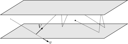
Figure 1.1: An idealized molecular flight between two solid plates, as an example of a multi-scattering experiment. We refer to $v$ and $V$, respectively, as the pre- and post-scattering velocities at a collision event, and regard $V$ as a random function of $v$, as explained in the text.

An example of a very simple interaction mechanism (in dimension $2$) is shown in Figure 3.1. That figure can be thought to represent a choice of wall “microstructure.” In addition to a choice of mechanical system representing the wall microstructure, the specification of a scattering map requires fixing a statistical kinetic state of this microstructure prior to each collision. For the example of Figure 3.1, one possible specification may be as follows: (1) the precise position on the horizontal axis (the dashed line of the figure) where the molecule enters the zone of interaction is random, uniformly distributed over the period of the periodic surface contour; (2) at the same time that the molecule crosses the dashed line (which arbitrarily sets the boundary of the interaction zone), the position and velocity of the up-and-down moving wall are chosen randomly from prescribed probability distributions. The most natural are the uniform distribution (over a small interval) for the position, and a one-dimensional normal distribution for the velocity, with mean zero and constant variance. (The variance specifies the wall temperature, as will be seen.) In fact, one general assumption of the main theorems essentially amounts to the constituent masses of the wall sub-system having velocities which are normally distributed and in a state of equilibrium (specifically, energy equipartition is assumed). In this respect, a random-mechanical model of “heat bath” is explicitly given. Once the random pre-collision conditions are set, the mechanical system describing the interaction evolves deterministically to produce $V$. Note that a single collision event may consist of several “billiard collisions” at the “microscopic level.”

Having specified a scattering map (by the choices of a mechanical system and the constant pre-collision statistical state of the wall), a random dynamical system on $\mathbb{H}$ is defined, which can then be studied from the perspective of the theory of Markov chains on general state spaces ([13]).

Clearly, one can equally well envision a multiple scattering set-up similar to the one depicted in Figure 1.1 but inside a cylindrical channel or a spherical container rather than two parallel plates; or, more generally, inside a solid container of irregular shape, in which case a “random change of frames” operator must be composed with the scattering operator to account for the changing orientation of the inner surface of the container at different collision points. (See [8]. This is not needed in the case of plates, cylinders, and spheres.) We like to think of this general set-up as defining a random billiard system, an idea that is nicely illustrated by [5, 6], for example.

We are particularly interested in situations that exhibit weak scattering, in the sense that the probability distribution of $V$ is concentrated near $v$ or, what amounts to the same thing, the scattering is nearly specular. Our systems will typically depend on a parameter $h$ that indicates the strength of the scattering, and we are mainly concerned with the limit of the velocity (Markov) process as $h$ approaches $0$. This will lead to novel types of diffusion processes canonically associated with the underlying mechanical systems. We call $h$ the flatness parameter for reasons that will soon become obvious.

For the systems of billiard type considered here (introduced in Section 2), the essential information concerning their mechanical and probabilistic definition is contained in two linear maps: $C$ and $\Lambda$ on $\mathbb{R}^{m+k}$, where $k$ is the number of “hidden” independent variables (whose statistical states are prescribed by the model) and $m$ is the number of “observed” variables (say, the $3$ velocity coordinates of the molecule in the situation of Figure 1.1). This $m$ is also the general dimension of $\mathbb{H}$. Vectors in $\mathbb{H}$ will be written $v=(v_{1},\dots,v_{m})$. The maps $C$ and $\Lambda$ are non-negative definite and Hermitian; $C$ is a covariance matrix for the hidden velocities and, by the equipartition assumption, it is a scalar multiple of an orthogonal projection, while $\Lambda$ contains (in the limit $h\rightarrow 0$) information about the system geometry and mass distribution.

The first observation (which is studied in much greater generality in [7]) is that the resulting Markov chain on velocity space $\mathbb{H}$ has canonical stationary distributions given by what we refer to as the post-collision Maxwell-Boltzmann distribution of velocities. (The term “post-collision” is used to distinguish it from the more commonly known distribution of velocities sampled at random times, not necessarily on the wall surface.) This velocity distribution has the form

(1.1) $$d\mu(v)=|v_{m}|\exp\left(-\frac{1}{2}|v|^{2}/\sigma^{2}\right)\,dV(v)$$

where $\sigma^{2}=\text{Tr}(C\Lambda)/\text{Tr}(\Lambda^{\curlywedge})$, $\Lambda^{\curlywedge}$ is the restriction of $\Lambda$ to the subspace of “hidden velocities,” and $dV$ denotes Euclidean volume element. The scattering map can be represented as a (very generally) self-adjoint operator on $L^{2}(\mathbb{H},\mu)$ of norm $1$, which we indicate by $P_{h}$, where $h$ is the flatness parameter. We denote the density of $\mu$ by $\varrho:=d\mu/dV.$ The term $|v_{m}|$ in $\varrho$ equals the speed times the cosine of the angle between $v$ and the normal to the scattering surface; this cosine factor is often referred to in the applied literature as the Knudsen cosine law. ([2])

Let $C_{0}^{\infty}(\mathbb{H})$ denote the space of compactly supported smooth functions on the half-space. A first order differential operator can be defined on this space using $C$ and $\Lambda$ as follows:

(1.2) $$\left(\mathcal{D}\Phi\right)(v):=\sqrt{2}\left[\Lambda^{1/2}\left(v_{m}\,\text{grad}_{v}\,\Phi-\Phi_{m}(v)v\right)+\text{Tr}\left(C\Lambda\right)^{1/2}\Phi_{m}(v)e\right]$$

where $e$ is the coordinate vector $(0,\dots,0,1)$ and the subindex $m$ in $\Phi_{m}$ indicates partial derivative with respect to $v_{m}$. We now define a second order differential operator on $C_{0}^{\infty}(\mathbb{H})$ by

$$\mathcal{L}:=-\mathcal{D}^{*}\mathcal{D},$$

where $\mathcal{D}^{*}$ indicates the adjoint of $\mathcal{D}$ with respect to the natural inner product on the pre-Hilbert space of smooth, compactly supported square integrable vector fields with the Maxwell-Boltzmann measure $\mu$. We refer to $\mathcal{L}$ as the MB-Laplacian of the mechanical-probabilistic model, $\mathcal{D}$ as the MB-gradient, and $-\mathcal{D}^{*}$ the MB-divergence.

The central result of the paper is that, as $h$ approaches $0$ (and under commonly satisfied further conditions to be spelled out later), the Markov chain process with transition probabilities operator $P_{h}$ converges to a diffusion process on $\mathbb{H}$ whose infinitesimal generator is the MB-Laplacian $\mathcal{L}$. The resulting process, which we call MB-diffusion, is illustrated in a number of concrete examples in the paper.

Figure 1.2: Sample trajectory of the MB-diffusion process whose infinitesimal generator is given by $(\mathcal{L}\Phi)(v)=-2v_{1}\Phi_{1}+\left[-4v_{2}+\left(1+v_{1}^{2}\right)/v_{2}\right]\Phi_{2}+v_{2}^{2}\Phi_{11}-2v_{1}v_{2}\Phi_{12}+(1+v_{1})\Phi_{22}$ obtained by simple Euler approximation. We have used a time interval of length $50$, initial condition $(0,-1)$ and number of steps $50000$. The parameters chosen here are not related to those of Figure 3.3, so the axis scales are not comparable.

The MB-diffusion can be expressed as an Itô stochastic differential equation

$$dV_{t}=Z(V_{t})\,dt+b(V_{t})\,dB_{t},$$

where $B_{t}$ is $m$-dimensional Brownian motion (restricted to $\mathbb{H}$), $Z(v)$ is the vector field

$$Z(v):=-2\Lambda v+({\varrho_{m}}/{\varrho})\left[\langle\Lambda v,v\rangle+\text{Tr}(C\Lambda)\right]e$$

and $b(v)$ is the linear map

$$b(v)u:=v_{m}\Lambda^{1/2}u-\langle\Lambda^{1/2}v,u\rangle e_{m}+\text{Tr}\left(C\Lambda\right)^{1/2}u_{m}e.$$

A sample path of an MB-diffusion in dimension $2$ is shown in Figure 1.2.

It is interesting to note that, in dimension $1$, the operator $\mathcal{L}$ reduces to the (up to a constant) Laguerre differential operator (in this case on functions defined on the interval $(-\infty,0)$):

$$\frac{1}{2\lambda\sigma^{2}}(\mathcal{L}\Phi)(v)=\frac{1}{\varrho}\frac{d}{dv}\left(\varrho\frac{d\Phi}{dv}\right),$$

where $\varrho(v)=\sigma^{-2}v\exp\left(-v^{2}/2\sigma^{2}\right)$ is the Maxwell-Boltzmann density and $\lambda$ is the scalar equal to the (in this case $1$-by-$1$) matrix denoted above by $\Lambda$.

Figure 1.3: Sample path for the Legendre diffusion in dimension $2$ with eigenvalues (of $\Lambda$) $\lambda_{1}=2.5$ and $\lambda_{2}=1$. The starting point is $(0,0)$, the time length is $5$, and the number of steps is $50000$. Note that diffusion is faster along the horizontal axis as $\lambda_{1}>\lambda_{2}$. The stationary distribution for this process is the normalized Lebesgue measure; therefore, long trajectories fill the disc evenly.

It has been implicitly assumed above that the number of independent “hidden” velocity components $k$ is positive. The case $k=0$ is somewhat different and has special interest. Now, particle speed does not change after scattering (we refer to this case as random elastic scattering) and both the Markov chain process and the diffusion approximation can be restricted to a unit hemisphere in $\mathbb{H}$. Alternatively, by orthogonal projection from the hemisphere to the unit open ball in dimension $m-1$, we can consider these processes taking place on the ball. Now $\mathcal{L}$ is completely determined by $\Lambda$ and has the form

$$(\mathcal{L}\Phi)(v)=2\sum_{i=1}^{n}\lambda_{i}\left((1-|v|^{2})\Phi_{i}\right)_{i}$$

where the $\lambda_{i}$ are the eigenvalues of $\Lambda$ and $\Phi$ is a compactly supported smooth function on the unit ball. (We have chosen coordinates adapted to the eigenvectors of $\Lambda$.)

The associated diffusion process, written as an Itô stochastic differential equation, has the form

$$dV_{t}=-4\Lambda V_{t}\,dt+\left[2\left(1-|V_{t}|^{2}\right)\Lambda\right]^{1/2}dB_{t},$$

where $B_{t}$ is $(m-1)$-dimensional Brownian motion restricted to the unit ball. The operator $\mathcal{L}$ in this case naturally generalizes the standard Legendre differential operator on the unit interval $(-1,1)$; we call the stochastic process on the higher dimensional balls Legendre diffusions. The stationary measure turns out to be standard Lebesgue measure on the ball, so Legendre diffusions have the interesting property that sample paths fill the ball uniformly with probability $1$. A sample path of a Legendre diffusion process is illustrated in Figure 1.3. One can also think of the Legendre diffusion as a special case of the MB-diffusion in the sense explained in Proposition 5 and in the remarks immediately after this proposition.

The relationship between the scattering operators $P$ and the above differential operators of Sturm-Liouville type suggests that one should be able fruitfully to investigate the spectral theory of $P$ based on an analysis of $\mathcal{L}$ and a spectral perturbation approach. A very simple observation in this regard is indicated in [9], while [10] discusses the spectral gap of $P$ (which can often be shown to be a Hilbert-Schmidt operator) in very special cases. We hope to turn to a more detailed analysis of the spectrum of $P$ in a future study.

2 Mechanical systems of billiard type

We introduce in this section the main definitions and basic facts concerning classical mechanical systems of billiard type and their derived random systems. Component masses of a given mechanical model interact via elastic scattering that admit a billiard representation. Particular attention is given to weak scattering, in which reflection in this billiard representation is nearly specular. A sequence of random scattering events comprises a Markov chain on velocity space whose transition probabilities operator, in the case of weak scattering, is close to the identity.

2.1 Deterministic scattering events

The reader may like to keep in view the examples of Figures 2.1 and 3.1 while reading the below definitions. For our purposes, a system of billiard type is a mechanical system defined by the geodesic motion of a point particle in a Riemannian manifold of dimension $n$ with piecewise smooth boundary. Upon hitting the boundary, trajectories reflect back into the interior of the manifold according to ordinary specular reflection and continue along a geodesic path. Except for passing references to more general situations, the configuration manifolds of the systems considered in this paper are Euclidean. More specifically, we consider $(n+1)$-dimensional submanifolds of $\mathbb{T}^{n}\times\mathbb{R}$ with boundary, for some $n$, with a Riemannian metric which will have constant coefficients with respect to the standard coordinate system. The boundary, assumed to be the graph of a piecewise smooth function, and the metric coefficients are the distinguishing features of each model. The periodicity implied by the torus factor is a more restrictive condition than really needed, but these manifolds are a natural first step and describe a variety of situations of special interest. Thus the configuration manifold $M$ is assumed to have the form

$$M=\{(x,x_{n+1})\in\mathbb{T}^{n}\times\mathbb{R}:x_{n+1}\geq F(x)\}$$

where $F$ is a piecewise smooth function.

The Riemannian metric on $M$ is specified by the kinetic energy quadratic form, which depends on the distribution of masses in the system. The Euclidean condition means, in effect, that the kinetic energy form becomes, after a linear coordinate change, the standard dot-product norm restricted to (the tangent bundle of) $M$, while the torus component of $M$ has the form $\mathbb{T}^{n}=\Pi_{i=1}^{n}\left(\mathbb{R}/a_{i}\mathbb{Z}\right)$ for positive constants $a_{1},\dots,a_{n}$.

A scattering event is defined as follows. Let $c$ be an arbitrary constant satisfying $F(x)<c$ for all $x\in\mathbb{T}^{n}$. The submanifold $x_{n+1}=c$ will be called the reference plane. We identify the tangent space to $M$ at any point on the reference plane with $\mathbb{R}^{n+1}$ and denote by $\mathbb{H}_{-}^{n+1}$ the lower-half space in $\mathbb{R}^{n+1}$, which consists of tangent vectors whose $(n+1)$st coordinate is negative.

Definition 1 (Deterministic scattering event).

A scattering event is an iteration of the correspondence $(x,v)\mapsto(x^{\prime},V)$, where $x,x^{\prime}$ lie on the reference plane and $(x^{\prime},V)$ is the end state of a billiard trajectory that begins at $x$ with velocity $v$ and ends at $x^{\prime}$ with velocity $V$. By reflecting $V$ on the reference plane, we may when convenient regard both $v$ and $V$ as vectors in $\mathbb{H}_{-}^{n+1}$.

Notice that the map describing a scattering event is indeed well defined, at least for almost all $(x,v)$, by Poincaré recurrence. If $|\text{grad}_{x}F|$ is uniformly small over $x\in\mathbb{T}^{n}$, a condition that is assumed in the main theorems, trajectories cannot get trapped.

The iteration of the scattering event map introduced in Definition 1, as well as its associated random maps described in Subsection 2.2, acquires greater significance in the context of random billiard systems as in [7], but the various concrete examples given later in this paper (the simplest of which appears in Subsection 2.3) should provide enough motivation.

2.2 Random systems and weak scattering

The random scattering set-up defined here is a special case of the one considered in [7]. Briefly, the main idea is that some of the variables involved in a deterministic scattering event, as defined above, are taken to be random. The scattering map then becomes a random function of the initial state of the system. The resulting random system can model a variety of physical situations; we refer to [7] for more details on the physical interpretation.

The notation $\mathcal{P}(X)$ will be used below to designate the space of probability measures on a measurable space $X$. We start with a deterministic scattering system with configuration manifold $M\subset\mathbb{T}^{n}\times\mathbb{R}$ and boundary function $F:\mathbb{T}^{n}\rightarrow\mathbb{R}$. Recall that $M$ is defined by the inequality $x_{n+1}\geq F(x)$, $x\in\mathbb{T}^{n}$. The deterministic scattering map is then $(x,v)\mapsto(x^{\prime},V)$, where $x,x^{\prime}$ lie on the reference plane $x_{n+1}=c$ (recall that $c$ is an essentially arbitrary value that specifies the reference plane); $v$ and $V$ lie in the lower-half space $\mathbb{H}_{-}^{n+1}$, and $V$ is the reflection on the reference plane of the velocity of the billiard trajectory with initial state $(x,v)$ at the moment the trajectory returns to the reference plane. A scattering event can consist of several billiard collisions.

Choose $c^{\prime}$ such that $\sup_{x}|F(x)|\leq c^{\prime}<c$ and define

$$M_{c^{\prime}}:=\{(x,x_{n+1})\in M:x_{n+1}>c^{\prime}\}=\mathbb{T}^{n}\times(c^{\prime},\infty).$$

Let $k\leq n$ be a non-negative integer and write $M_{c^{\prime}}=\mathbb{T}^{k}\times\mathbb{T}^{n-k}\times(c^{\prime},\infty)$. Accordingly, decompose the tangent space to $M$ at any point on the reference plane as $\mathbb{H}^{n+1}_{-}=\mathbb{R}^{k}\times\mathbb{H}_{-}^{n-k+1}$. Fix a probability measure $\mu$ on $\mathbb{R}^{k}$ and set $m=n-k+1$. By a random initial state with observable component $v\in\mathbb{H}_{-}^{m}$ we mean a state of the form $(x,c,w,v)$, where $x\in\mathbb{T}^{n}$ is a uniformly distributed random variable, $c$ is the value defining the reference plane, and $w$ is a random variable taking values in $\mathbb{R}^{k}$ with probability measure $\mu$. To this random initial state we can associate a probability measure $\nu_{v}\in\mathcal{P}(\mathbb{H}^{m}_{-})$ as follows: Consider the trajectory of the system of billiard type having random initial state $(x,c,w,v)$, and let $V$ be the component in $\mathbb{H}_{-}^{m}$ of the final velocity of this trajectory, reflected back into $\mathbb{H}_{-}^{m}$, at the moment the trajectory returns to the reference plane. Then $V$ is a random variable and $\nu_{v}$ is by definition its probability measure. We refer to $\nu_{v}$ as the return probability distribution associated to the random initial state having observable component $v$.

Definition 2 (Random scattering event).

Let $\mu$ be a probability measure on $\mathbb{R}^{k}$ and give $\mathbb{T}^{n}$ the uniform probability measure, denoted $\lambda$. Then the random scattering event associated to the system of billiard type and these fixed measures is defined by the map

$$v\in\mathbb{H}^{m}_{-}\rightarrow\nu_{v}\in\mathcal{P}(\mathbb{H}^{m}_{-}),$$

where $\nu_{v}$ is the return probability associated to the random initial state with observable component $v$.

The probability measure $\mu$ on $\mathbb{R}^{k}$ typically will be assumed to have zero mean, non-singular covariance matrix of finite norm, and finite moments of order $3$, when not assumed more concretely to be Gaussian. The uniform distribution on $\mathbb{T}^{n}$ is, by definition, the unique translation invariant probability measure.

Definition 3 (Scattering operator $P$).

Let $C_{0}(\mathbb{H}_{-}^{m})$ denote the space of compactly supported continuous functions on the lower half-space. For any given $\Phi\in C_{0}(\mathbb{H}_{-}^{m})$, define

$$(P\Phi)(v):=\int_{\mathbb{R}^{k}}\int_{\mathbb{T}^{n}}\Phi(V(x,c,v,w))\,d\lambda(x)\,d\mu(w).$$

We call $P$ the scattering operator of the system for a random initial state specified by $\mu$ and the uniform distribution on the torus.

Operators similar to our $P$ naturally arise in kinetic theory of gases and are used to specify boundary conditions for the Boltzmann equation. See, e.g., [1, 11]. Typically, the models of gas surface interaction used in the Boltzmann equation literature are phenomenological, such as the Maxwell model ([1], Equation 1.10.20), and are not derived from explicit mechanical interaction models as we are interested in doing here.

From the definitions it follows that $P$ and $\nu_{v}$ are related by

$$(P\Phi)(v)=E_{v}[\Phi(V)]=\int_{\mathbb{H}_{-}^{m}}\Phi(u)\,d\nu_{v}(u)$$

where the expression in the middle denotes the expectation of the random variable $\Phi(V)$ given the initial condition $v$.

Based on the examples given throughout the paper, we can expect $P$ and $v\mapsto\nu_{v}$ generally to have good measurability properties, due to the deterministic map from which the random process is defined being typically piecewise smooth. In our general theorems it will be implicitly assumed that $v\mapsto\nu_{v}(A)$ is Borel measurable for all Borel measurable subsets $A$ of $\mathbb{H}_{-}^{m}$. Billiard maps are typically not continuous; see [3] for basic facts on billiard dynamics (in dimension $2$).

The following additional assumption turns out to be convenient and not too restrictive.

Definition 4 (Symmetric $M$, $F$).

The configuration manifold $M$ of a random scattering process or, equivalently, the function $F$ defining it, will be called symmetric if $F(o+u)=F(o-u)$ for all $u\in\mathbb{R}^{n}$ and some choice of origin $o$ in $\mathbb{T}^{n}$.

2.3 Example: collision of a rigid body and flat floor

A simple example will help to clarify and motivate some of the above definitions. (More representative examples will be introduced later.) Consider the $2$-dimensional system of Figure 2.1. It consists of a rigid body in dimension $2$ of constant density and mass $m$ that moves in the half-plane set by a hard straight floor. There are no potentials (e.g., gravity). The body and floor surfaces are assumed to be physically smooth, in the sense that there is no change in the component of the linear momentum tangential to the floor after a collision. The motion of the center of mass can then be restricted to the dashed line of Figure 2.1 due to conservation of the horizontal component of the linear momentum.

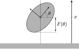
Figure 2.1: Collision of a rigid body and a flat floor in dimension $2$. The shape of the body is encoded in the function $F(\theta)$. For a disc, $F$ is constant. Some of the main results of the paper apply to shapes for which $h:=\sup_{\theta}\left(F^{\prime}(\theta)\right)^{2}$ is small.

Figure 2.2 shows the description of the same example explicitly as a system of billiard type. Let $B$ represent the body at a fixed position, with its center of mass at the origin. Define the second moment of the position vector by $l^{2}:=\text{Area}^{-1}\int_{B}|b|^{2}\,dA(b)$, where $A$ is the area measure. Set coordinates $x_{1}=\theta$ and $x_{2}=x/l$, where $\theta$ is the angle of rotation and $x$ is the height of the center of mass of the body at a given configuration in $\mathbb{R}^{2}$. Then the configuration manifold of the system is the region $M=\{(x_{1},x_{2})\in\mathbb{T}\times\mathbb{R}:F(x_{1})\leq lx_{2}\},$ equipped with the kinetic energy metric $K=\kappa\left(\dot{x}_{1}^{2}+\dot{x}_{2}^{2}\right)$, where $\kappa$ is a positive constant. We model the collision between the body and the floor by a linear map $C:T_{x}M\rightarrow T_{x}M$, where $x$ is a boundary (collision) point of $M$. Under the assumption of energy conservation and time reversibility, $C$ is an orthogonal involution; the assumption of physically smooth contact is interpreted as $Cu=u$ for every nonzero vector $u$ tangent to the boundary at $x$. As $C$ cannot be the identity map, it must be standard Euclidean reflection, whence the system is of billiard type.

The $3$-dimensional version of this example is similarly described, the function $F$ now being defined on the special orthogonal group $\text{SO}(3)$. The kinetic energy metric on $M\subset\text{SO}(3)\times\mathbb{R}$ is no longer Euclidean and naturally involves the body’s moment of inertia.

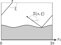
Figure 2.2: The billiard representation associated to the mechanical system of Figure 2.1. Here $M\subset\mathbb{T}\times\mathbb{R}$. (Dashed lines indicate periodic conditions.) The reference plane is indicated by the top horizontal line and the wavy ground is the graph of $F$. We define the pre-scattering angle $\xi$ and initial position $s\in[0,2\pi]$. The outgoing angle is $\Xi$.

One way in which this deterministic system can be turned into an example of a random system is by regarding the initial angle $\theta$, at the moment the center of mass of the body crosses a reference plane, to be random with the uniform distribution over the interval $[0,2\pi]$. In other words, suppose that the exact orientation of the body in space at a given moment prior to collision is completely unknown. As the magnitude of the velocity of the billiard particle (that is, of the moving point particle of Figure 2.2) is invariant throughout the process due to energy conservation, we may consider the return probability as being supported on the half-circle in $\mathbb{H}^{2}_{-}$, which we identify with the interval of angles $[0,\pi]$.

Thus the probability distribution $\nu_{\xi}$ of the return angle $\Xi$ given $\xi$ is the measure:

$$U\mapsto\nu_{\xi}(U)=\frac{1}{2\pi}\int_{0}^{2\pi}\mathbbm{1}_{U}\left(\Xi(s,\xi)\right)\,ds$$

where $U$ is a measurable subset of the interval $[0,\pi]$ (a set of scattered angles) and $\mathbbm{1}_{U}$ is the indicator function of $U$. Similarly, given a continuous function $\Phi$ on $[0,\pi]$,

$$(P\Phi)(\xi)=\frac{1}{2\pi}\int_{0}^{2\pi}\Phi\left(\Xi(s,\xi)\right)\,ds=\int_{0}^{\pi}\Phi(\Xi)\,\nu_{\xi}(\Xi).$$

The probability distributions of the velocity of the center of mass and the angular velocity (expressed in terms of $\dot{x}_{2}$ and $\dot{x}_{1}$, respectively) are obtained by taking the push-forward of $\nu_{\xi}$ under the maps $u\mapsto|\xi|\cos(u)$ and $u\mapsto|\xi|\sin(u)$, respectively. Note that $\nu_{\xi}$ approaches weakly the delta measure $\delta_{\xi}$ supported on $\xi$ when the body becomes more and more round (hence the reflecting line in Figure 2.2 becomes more and more straight). In this case, $P$ approaches the identity operator.

2.4 Further notations

All the examples of deterministic systems given in this paper can be turned into random scattering systems in various ways. The most natural choices of random variables fall within the scope of the following discussion, in which the definition of a random scattering event is restated in a more convenient form. Let the tangent space to $M$ at any point $(x,c)$ of the reference plane decompose in the following two different ways:

$$\mathbb{H}_{-}^{n+1}=\mathbb{R}^{k}\times\mathbb{H}^{m}=\mathbb{R}^{n}\times(-\infty,0).$$

where $m=n-k+1$. Accordingly, any given $\xi\in T_{x}M$ has components relative to these two decompositions defined by

$$\xi=(\xi^{\curlywedge},\xi^{\curlyvee})=(\overline{\xi},\xi_{n+1}).$$

Let $\{e_{1},\dots,e_{n+1}\}$ be the standard basis of $\mathbb{R}^{n+1}$ and $e:=e_{n+1}$ the last basis vector. So

$$\xi_{n+1}=\langle\xi,e\rangle,\ \ \xi^{\curlywedge}=\sum_{i=1}^{k}\langle\xi,e_{i}\rangle e_{i},\ \ \xi^{\curlyvee}=\xi-\xi^{\curlywedge}$$

where the inner product represented by the angle brackets is the standard dot product. The component $\xi^{\curlyvee}$ of the final velocity of the billiard trajectory is the quantity of interest produced by the scattering event. The component $\xi^{\curlywedge}$ of the initial velocity is assumed random with a probability distribution $\mu$.

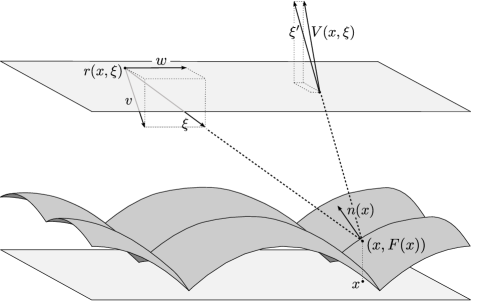
Figure 2.3: The random collision process. The initial position $r\in\mathbb{T}^{n}\times\{c\}$ on the reference plane is chosen randomly with the uniform distribution. The outgoing velocity in $TM$ is $\xi^{\prime}$, and the vertical projection $V:=\xi^{\curlyvee}$ is the outgoing observed velocity. We thus obtain a random map $v\mapsto V$. It will turn out to be convenient to express both $r$ and $V$ in terms of $\xi$ and the independent variable $x\in\mathbb{T}^{n}$, as indicated in the figure.

We can now express the random scattering map $v\mapsto V$ by the following algorithm, which is illustrated in Figure 2.3.

Definition 5 (Random scattering algorithm).

In the notation introduced above, the random scattering map is defined by the following steps:

1. Start with $v\in\mathbb{H}_{-}^{m}$;

2. Choose a random $w\in\mathbb{R}^{k}$ with the probability distribution $\mu$ and form $\xi:=w+v$;

3. Choose a random $r=(\overline{r},c)$, where $\overline{r}\in\mathbb{T}^{n}$ is uniformly distributed, and let $(r,\xi)$ be the initial state for the billiard trajectory;

4. Let $\xi^{\prime}\in\mathbb{H}_{-}^{n+1}$ be the velocity of the billiard trajectory at the time of its return to $r_{n+1}=c$;

5. Set $V:=(\xi^{\prime})^{\curlyvee}\in\mathbb{H}_{-}^{m}$.

For billiard surfaces (i.e., the graph of $F$) that are relatively flat, the typical collision process comprises a single collision. It makes sense in this case to introduce the independent variable $x$ as indicated in Figure 2.3, and allow both $\overline{r}$ and $\xi^{\prime}$ to be functions of $x$ and $\xi$. For $x\in\mathbb{T}^{n}$, let $n(x)$ be the unit normal vector to the graph of $F$ at $(x,F(x))$. Note that

$$n(x)=\frac{e-\text{grad}_{x}F}{\sqrt{1+\|\text{grad}_{x}F\|^{2}}}.$$

As a geometric measure of the strength of scattering we introduce the following parameter.

Definition 6 (Flatness parameter).

The quantity $h:=\sup_{x\in\mathbb{T}^{n}}|\text{\em grad}_{x}F|^{2}$ will be referred to as the flatness parameter of the system defined by $F$.

3 Stationary measures and general properties of $P$

The basic properties of $P$ are described in this section. These are mostly special cases of results from [7], which we add here for easy reference. Proofs are much simpler in our present setting and are sketched here.

3.1 Stationary measures

It will be assumed in much of the rest of the paper that the probability distribution $\mu$ for the velocity component $w$ in $\mathbb{R}^{k}$, when $k>0$, is Gaussian:

$$d\mu(w)=\frac{e^{-\frac{1}{2}|w|^{2}/\sigma^{2}}}{\left(2\pi\sigma^{2}\right)^{k/2}}dV(w)$$

occasionally referring to $\sigma^{2}$ as the temperature (of the “hidden state”). Let $\lambda$ be the translation invariant probability measure on $\mathbb{T}^{n}$. The standard volume element in open subsets of Euclidean space will be written $dV$, or $dV^{k}$ if we wish to be explicit about the dimension.

Recall that the deterministic scattering map $T$ is defined as the return billiard flow map on the phase space restricted to the reference plane, that is, $\mathbb{T}^{n}\times\mathbb{H}_{-}^{n+1}=\left(\mathbb{T}^{n}\times\mathbb{R}^{k}\right)\times\mathbb{H}_{-}^{m}$, where we are factoring out the observable velocity component $\mathbb{H}^{m}$ from the hidden component at temperature $\sigma^{2}$, which is given the probability distribution $\nu:=\lambda\otimes\mu$ in the sense described in the previous section. Denote by $\pi$ the natural projection $\pi:\mathbb{T}^{n}\times\mathbb{R}^{k}\times\mathbb{H}_{-}^{m}\rightarrow\mathbb{H}_{-}^{m}$

When $k=0$ (no velocity components among the hidden variables), the scattering interaction does not change the magnitude of the velocity in $\mathbb{H}_{-}^{m}$; thus one may restrict the state to the unit hemisphere $S_{-}^{m-1}$ in $\mathbb{H}^{m}_{-}$. Let $d\omega(u)$ represent the Euclidean volume element (measure) on the hemisphere at the unit vector $u$. When necessary we indicate the dimension of the unit hemisphere as $d\omega^{m-1}$. Observe that

$$dV^{m}(v)=c|v|^{m-1}\,d\omega^{m-1}(v/|v|)\,d|v|,$$

where $c$ is $m$ times the ratio of the volume of the unit $m$-ball by the volume of the unit $(m-1)$-sphere.

The Markov operator $P$ naturally acts on probability measures on $\mathbb{H}_{-}^{m}$ as follows. With the notation $\eta(f):=\int f\,d\eta$, the action of $P$ on $\eta$ is the measure $\eta P$ such that $(\eta P)(f)=\eta(Pf)$, for every compactly supported continuous $f$. A probability measure $\eta$ on $\mathbb{H}_{-}^{m}$ is said to be stationary for a Markov operator with state space $\mathbb{H}_{-}^{m}$ if $\eta P=\eta$.

The action of $P$ on probability measures has the following convenient expression. Given any probability measure $\eta$ on $\mathbb{H}_{-}^{m}$, we can form the probability measure $\nu\otimes\eta$ on $(\mathbb{T}^{n}\times\mathbb{R}^{k})\times\mathbb{H}_{-}^{m}$, then act on this measure by the push-forward operation $T_{*}$ under the return map, and finally project the resulting probability measure back to $\mathbb{H}_{-}^{m}$. (We recall that $T_{*}\zeta$, for a given measure $\zeta$, can be defined by its evaluation on continuous functions as $(T_{*}\zeta)(f):=\zeta(f\circ T)$.) The result is $\eta P$.

Lemma 1.

The operation $\eta\mapsto\eta P$ for $\eta\in\mathcal{P}\left(\mathbb{H}_{-}^{m}\right)$ can be expressed as

$$\eta P=(\pi\circ T)_{*}(\nu\otimes\eta),$$

where $\nu=\lambda\otimes\mu$ is the fixed probability on the hidden variables space $\mathbb{T}^{n}\times\mathbb{R}^{k}$, $T$ is the return map to the phase space restricted to reference plane, identified with $\mathbb{T}^{n}\times\mathbb{R}^{k}\times\mathbb{H}_{-}^{m}$, and $\pi$ is the projection from this phase space to $\mathbb{H}_{-}^{m}$.

Proof.

The straightforward proof amounts to interpreting the definition of $P$ given earlier in terms of the push-forward notation. See [7] for more details. ∎

Proposition 1.

When $k=0$, the measure $d\eta(v)=\langle v,e\rangle\,d\omega(v)$ defined on the unit hemisphere in $\mathbb{H}_{-}^{m}$ is stationary under $P$. Identifying the unit hemisphere with $D_{1}^{m-1}=\{x\in\mathbb{R}^{m-1}:|x|<1\}$ under the linear projection $(x,x_{m})\mapsto x$, the stationary probability is, in this case, the normalized Lebesgue measure on $D_{1}^{m-1}$. For $k>0$, the measure

$$d\eta(v)=|\langle v,e\rangle|e^{-\frac{1}{2}|v|^{2}/\sigma^{2}}\,dV^{m}(v)$$

on $\mathbb{H}_{-}^{m}$ is stationary under $P$.

Proof.

For a much more general result see [7]. We briefly show here the second claim. First note that the measure $d\zeta_{0}(\xi):=\langle\xi,e\rangle\,d\lambda(x)\,dV(\xi)$ on $\mathbb{T}^{n}\times\mathbb{H}_{-}^{n+1}$ is $T$-invariant. (The term $\langle\xi,e\rangle$ contains the cosine factor that appears in the canonical invariant measure of billiard systems in general dimension.) The measure $d\zeta(\xi)=\exp(-\frac{1}{2}|\xi|^{2}/\sigma^{2})\,d\eta_{0}(\xi)$ is also $T$-invariant, since any function of $|\xi|$ is invariant under the return map $T$. Now, consider the decomposition $\xi=(x,w,v)\in\mathbb{T}^{n}\times\mathbb{R}^{k}\times\mathbb{H}_{-}^{m}$, under which $\zeta$ splits as $\zeta=\nu\otimes\eta$, where

$$d\eta(v)=|\langle v,e\rangle|e^{-\frac{1}{2}|v|^{2}/\sigma^{2}}\,dV^{m}(v).$$

Here we have used: $\langle\xi,e\rangle=\langle v,e\rangle$ and the splitting of the exponential involving $|\xi|^{2}=|w|^{2}+|v|^{2}$ as a product of exponentials in $w$ and $v$. Thus $\pi_{*}\zeta=\eta$, where $\pi_{*}$ indicates the push-forward operation on probability measures. We now apply Lemma 1, noting that $T_{*}\zeta=\zeta$, to obtain

$$\eta P=(\pi\circ T)_{*}(\nu\otimes\eta)=\pi_{*}T_{*}\zeta=\pi_{*}\zeta=\eta,$$

which is the claim. ∎

There is a significant literature in both pure mathematics and physics/engineering concerning random billiards, in which ordinary specular billiard reflection is replaced with a random reflection. The typical assumption is that the post-collision velocity distribution corresponds to the above Maxwellian distribution or, more simply, to the Knudsen cosine law with constant speed. See, for example, [2, 5, 6].

It is natural to regard $P$ as an operator on the Hilbert space $L^{2}(\mathbb{H}_{-}^{m},\eta)$ of square integrable functions on the observable factor with the stationary measure given in Proposition 1. The next (easy) proposition is proved in [7].

Proposition 2.

Suppose that the billiard system is symmetric, as defined in Definition 4, and let $\eta$ be one of the stationary measures described in Proposition 1. Then $P:L^{2}(\mathbb{H}_{-}^{m},\eta)\rightarrow L^{2}(\mathbb{H}_{-}^{m},\eta)$ is a self-adjoint operator of norm $1$.

3.2 Example: collision between particle and moving surface

The example discussed here is the simplest that exhibits most of the features of the general case. Its components are a point mass $m_{1}$ and a wall that is allowed to move up and down. See Figure 3.1. The wall surface, which could be of any dimension $n\geq 0$, has a periodic, piecewise smooth contour and the up and down motion is restricted to an interval $[0,a_{0}/2]$. In the interior of this interval the wall moves freely, bouncing off elastically at the heights $0$ and $a_{0}/2$. Collisions between the wall and mass $m_{1}$ are also elastic.

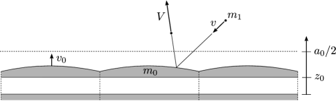
Figure 3.1: Collision between the surface of a moving rigid wall and a point mass $m_{1}$. The entire wall is given a certain mass $m_{0}$; models with more localized mass definition are also possible.

Let $x$ denote the coordinate along the (horizontal) base of the wall and let $z_{0}$ be the height at which the base stands at any given moment relative to its lowest position. The range of $z_{0}$ is assumed to be $[0,a_{0}/2]$. The contour of the wall top surface, when $z_{0}=0$, is described by a periodic function $f(x)$ of period $a_{1}$. Thus, when the base is at height $z_{0}$, that contour is the graph of $x\mapsto f(x)+z_{0}$. It is convenient to allow $z_{0}$ to vary over the symmetric interval $[-a_{0}/2,a_{0}/2]$ and set the wall surface function of $x,z_{0}$ as $G(z_{0},x)=f(x)+|z_{0}|$, which can then be extended periodically over $\mathbb{R}^{2}.$ The graph of $G$ so extended is, up to a rescaling of the coordinates to be described shortly, the surface shown in Figure 3.2. Periodicity of $G$ is expressed by $G(x+ma_{1},z_{0}+na_{0})=G(x,z_{0})$ for integers $m,n$. Equivalently, we think of $G$ as a function on the $2$-torus.

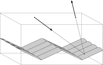
Figure 3.2: Billiard representation for the moving wall example.

The coordinates of the point mass $m_{1}$ are represented by $(z_{1},z_{2})$ respectively along and perpendicular to the base line of the wall. Thus the state of the system at any moment is specified by $(z_{0},z_{1},z_{2},v_{0},v_{1},v_{2})$, where $v_{0}$ is the velocity of $m_{0}$ and $v=(v_{1},v_{2})$ is the velocity of $m_{1}$.

An appropriate choice of coordinates makes the kinetic energy metric explicitly Euclidean. Set $x=(x_{0},x_{1},x_{2})$, where $x_{0}:=\sqrt{{m_{0}}/{m_{1}}}{z_{0}}/{a_{1}},\ x_{1}:={z_{1}}/{a_{1}},\ x_{2}:={z_{2}}/{a_{1}}.$ The above function $G$ in this new system becomes

$$F(x_{0},x_{1})=a_{1}^{-1}f\left(a_{1}x_{1}\right)+\sqrt{{m_{1}}/{m_{0}}}|x_{0}|.$$

Defining $\tau:=\frac{a_{0}}{a_{1}}\sqrt{\frac{m_{0}}{m_{1}}}$, then $F\left(x_{0}+m\tau,x_{1}+n\right)=F(x_{0},x_{1})$ for integers $m,n$. The configuration manifold of the particle-movable wall system can now be written in terms of $F$ as

$$M=\{x\in\mathbb{R}^{3}:x_{2}\geq F(x_{0},x_{1})\}.$$

The kinetic energy of the system then becomes $K(x,\dot{x})=K_{0}\|\dot{x}\|^{2},$ where $K_{0}=m_{1}a_{1}^{2}/2$. Under the assumption that the wall surface is physically smooth, we obtain again a system of billiard type in $M$, as depicted in Figure 3.2.

A random billiard scattering process based on the above set up can now be defined as follows. The observable state space is the set $\mathbb{H}_{-}^{2}$ of approaching velocities, consisting of the vectors $u_{1}e_{1}+u_{2}e_{2}$, $u_{2}<0$. The part of the phase space of the deterministic process on which the return map $T$ is defined is $\mathbb{T}^{2}\times\{0\}\times\mathbb{R}\times\mathbb{H}_{-}^{2}$. Observe that $\mathbb{T}^{2}=(\mathbb{R}/\tau\mathbb{Z})\times(\mathbb{R}/\mathbb{Z})$ has coordinate functions $(x_{0},x_{1})$, and the reference plane, with equation $x_{2}=0$, is identified with $\mathbb{T}^{2}$. At the initial moment of the scattering event it is assumed that the height of the wall ($x_{0}$) and the position of $m_{1}$ along a period interval of the wall contour ($x_{1}$) are random uniformly distributed over the respective ranges. Thus the initial position on $\mathbb{T}^{2}$ is a random variable distributed according to the normalized translation-invariant measure.

Also at the initial moment of the scattering event the velocity of the wall is assumed to be a Gaussian random variable with zero mean and variance $\sigma_{0}^{2}$. That is, the initial derivative $w:=\dot{x}_{0}$ of $x_{0}$ is normally distributed with mean $0$ and variance $\sigma^{2}=\frac{m_{0}}{m_{1}}\frac{\sigma_{0}^{2}}{a_{1}^{2}}$. Thus the probability distribution for $w$ is given by the measure $\mu$ such that $d\mu(w)=(2\pi\sigma^{2})^{-1/2}{e^{-\frac{1}{2}w^{2}/\sigma^{2}}}\,dw.$ In the original coordinate $v_{0}$ for the velocity of the wall, the distribution is

$$d\mu(v_{0})=\sqrt{\frac{m_{0}\beta}{2\pi}}e^{-\frac{\beta}{2}m_{0}v_{0}^{2}}\,dv_{0},$$

where $\beta^{-1}:=m_{0}\sigma_{0}^{2}$.

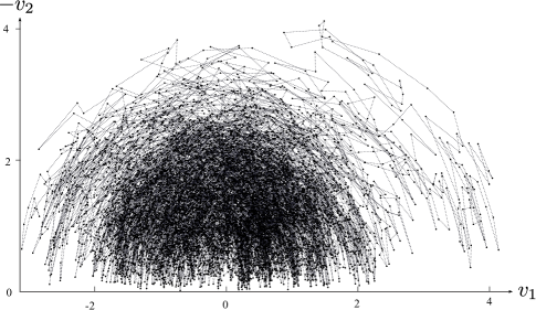
Figure 3.3: A typical trajectory of the Markov chain for the random scattering process of Figure 3.1. The parameters are given in the text.

The random scattering map given in Definition 5 generates a random dynamical system on $\mathbb{H}_{-}^{m}$ whose orbits are equivalently described as sample paths of a Markov chain process with state space $\mathbb{H}_{-}^{m}$. One way to interpret such multi-scattering process is to imagine that a point mass $m_{1}$ undergoes a random flight inside a long channel bounded by two parallel lines (the channel walls), these walls having at close range (compared to the distance between the two lines) the structure depicted in Figure 3.1.

Figure 3.3 shows a typical sample path of the multi-scattering Markov chain obtained numerically for the contour function $f(z_{1})=\sqrt{R^{2}-z_{1}^{2}}-\sqrt{R^{2}-a_{1}^{2}/4}$, with $a_{1}=1$, $R=4$, and masses $m_{0}=80$ and $m_{1}=1$. The variance is $\sigma_{0}=1$ and the number of iterations is $10^{4}$. (In the figure we used $-v_{2}$, so the trajectory is shown in the upper-half plane.)

According to Proposition 1, the stationary probability distribution for $u=(\dot{x}_{1},\dot{x}_{2})$ is

(3.1) $$d\eta(u)=\frac{1}{\sigma^{3}\sqrt{2\pi}}u_{2}e^{-\frac{1}{2}|u|^{2}/\sigma^{2}}\,du_{1}\,du_{2}.$$

Expressed in the original velocity variables $v_{1},v_{2}$ of $m_{1}$, this distribution has the form

(3.2) $$d\eta(v)=\frac{\left(m_{1}\beta\right)^{3/2}}{\sqrt{2\pi}}v_{2}e^{-\frac{\beta}{2}m_{1}|v|^{2}}\,dv_{1}\,dv_{2}=\left(\sqrt{\frac{2}{\pi}}\left(m_{1}\beta\right)^{3/2}s^{2}e^{-\frac{\beta}{2}m_{1}s^{2}}\,ds\right)\left(\frac{1}{2}\cos\theta\,d\theta\right)$$

where $s=|v|$ is the speed of $m_{1}$ and $\theta$ is the angle the velocity of $m_{1}$ makes with the normal to the reference plane pointing into the region of interaction. The fact that $\beta$ is the same in both distributions of velocities (for $m_{0}$ and $m_{1}$) is indicative of (thermal) equilibrium. These distributions are illustrated in Figure 3.4.

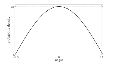
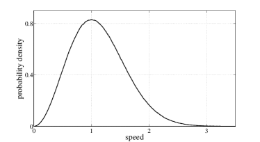
Figure 3.4: Factor densities of the stationary distribution $d\eta$ of scattered angle (left) and speed (right) as given on the right of 3.2 above, obtained by numerical simulation of the random billiard using a sample run of the Markov chain of length $10^{7}$. The parameters are $m_{0}=m_{1}=1$, $\sigma_{0}^{2}=1/2$, $f(z_{1})=\sqrt{R^{2}-z_{1}^{2}}-\sqrt{R^{2}-a_{1}^{2}/4}$ (an arc of circle) with $a_{1}=1$ and $R=3$. The analytically derived expressions for the distributions are also shown above (dashed lines) but are virtually indistinguishable from those obtained numerically (solid lines).

4 Differential approximation of the scattering operator

In this section we denote the scattering operator by $P_{h}$, indexed by the flatness parameter $h$, and define for all $\Phi$ in the space of compactly supported bounded functions $C_{0}^{\infty}(\mathbb{H}_{-}^{m})$

$$\mathcal{L}_{h}\Phi:=\frac{P_{h}\Phi-\Phi}{h}.$$

Other choices of denominator can be more natural or convenient in specific cases, but $h$ indicates the correct order of magnitude. Our immediate task is to describe a second order differential operator $\mathcal{L}$ to which $\mathcal{L}_{h}$ converges uniformly when applied to elements of $C_{0}^{\infty}(\mathbb{H}_{-}^{m})$.

4.1 Definitions, notations, and preliminary remarks

The notations used below were introduced in Subsection 2.4 and are summarized in Figure 2.3. In addition, we occasionally use the shorthand $\xi_{\smalltriangledown}:=\overline{\xi}/\langle\xi,e\rangle$. Also, the variable $r=(\overline{r},c)$ will typically be used to represent the initial position of trajectories, instead of $(x,c)$. Given an initial state $(r,\xi)$ with $r$ on the reference plane, let $V=V(r,\xi)$ denote the component in $\mathbb{H}_{-}^{m}$ of the velocity of the return state $T(r,\xi)$. Recall that, at the end point, the scattering map reflects the velocity back into $\mathbb{H}_{-}^{n+1}$. For trajectories that collide only once with the graph of $F$, it will be convenient to introduce the independent variable $x\in\mathbb{T}^{n}$ as indicated in Figure 2.3, and use it to express both $\overline{r}$ and $V$ for a given $\xi$, instead of writing $V(\overline{r},\xi)$ directly. Note that

$$\overline{r}(x,\xi)=x+(c-F(x))\xi_{\smalltriangledown},$$

whose differential in $x$ is $d\overline{r}_{x}=I-dF_{x}\otimes\xi_{\smalltriangledown}$. By a standard determinant formula,

(4.1) $$\det(d\overline{r}_{x})=1-{dF_{x}(\xi_{\smalltriangledown}})=1+{\langle n_{\smalltriangledown}(x),\xi_{\smalltriangledown}\rangle}.$$

Recall that $h$ is the supremum over $\mathbb{T}^{n}$ of $|\text{grad}_{x}F|^{2}$. We wish to study the scattering process for small values of $h$.

Lemma 2.

Let $\xi:=v+w\in\mathbb{H}_{-}^{m}\times\mathbb{R}^{k}$ be such that the trajectory with initial state $(\overline{r},c,\xi)$ collides with the graph of $F$ only once for all $\overline{r}\in\mathbb{T}^{n}$. We regard $\overline{r}$ as a function of the initial velocity and a point $x\in\mathbb{T}^{n}$, as indicated in Figure 2.3. Let $V=V(x,v,w)$ be the component in $\mathbb{H}_{-}^{m}$ of the velocity of the billiard trajectory as it returns to the reference plane after one iteration of the scattering map. Then $V=v+2\zeta_{1}-2\zeta_{2}$, where

$$\zeta_{1}(x,v,w) :=\langle n(x),e\rangle\left(\langle\overline{n}(x),{v}\rangle e+\langle\overline{n}(x),w\rangle e-\langle v,e\rangle\overline{n}^{\curlyvee}(x)\right)$$

$$\zeta_{2}(x,v,w) :=\langle\overline{n}(x),{v}\rangle\overline{n}^{\curlyvee}(x)+\langle\overline{n}(x),w\rangle\overline{n}^{\curlyvee}(x)+|\overline{n}(x)|^{2}\langle v,e\rangle e.$$

If $F$ is symmetric, these functions satisfy $\zeta_{1}(-x,v,w)=-\zeta_{1}(x,v,w)$, $\zeta_{2}(-x,v,w)=\zeta_{2}(x,v,w)$.

Proof.

This is an entirely straightforward calculation, of which we indicate a few steps. The reflection of $\xi$ after the single collision with the graph of $F$ at $x\in\mathbb{T}^{n}$ is naturally given by $\xi^{\prime}=\xi-2\langle n(x),\xi\rangle n(x)\in\mathbb{H}_{+}^{n+1}$. This is then reflected by a plane perpendicular to $e$, resulting in

$$\eta=\xi^{\prime}-2\langle\xi^{\prime},e\rangle e=\xi+2\langle n,e\rangle\left(\langle\overline{n},\overline{\xi}\rangle e-\langle\xi,e\rangle\overline{n}\right)-2\left(\langle\overline{n},\overline{\xi}\rangle\overline{n}+|\overline{n}|^{2}\langle\xi,e\rangle e\right)\in\mathbb{H}_{-}^{n+1}.$$

Now apply the linear projection ${\eta}\mapsto\eta^{\curlyvee}$ and use that $\langle\xi,e\rangle=\langle v,e\rangle$ and $\langle\overline{n},\overline{\xi}\rangle=\langle\overline{n},v\rangle+\langle\overline{n},w\rangle$ to obtain the stated identity relating $V$ and $v$. For the rest, use $\langle n(-x),e\rangle=\langle n(x),e\rangle$ and $\overline{n}(-x)=-\overline{n}(x)$. ∎

Lemma 3.

Define $W(v,h):=-|v|+{|\langle v,e\rangle|}/{4\sqrt{h}}$. Then for small enough $h$ (e.g., $h\leq(3/4)^{2}$), for all $x\in\mathbb{T}^{n}$ and all $\xi$ in the set

$$\mathcal{D}_{h}:=\left\{v+w\in\mathbb{H}^{n+1}_{-}:|w|<W(v,h)\right\}$$

the trajectory with initial vector $\xi$ starting at $(\overline{r}(x,\xi),c)$ collides with the graph of $F$ only once and the Jacobian determinant of $x\mapsto\overline{r}(x,\xi)$ satisfies $\det(d\overline{r}_{x})=1+\langle n_{\smalltriangledown}(x),\xi_{\smalltriangledown}\rangle>0$.

Proof.

Let $\xi^{\prime}:=\xi-2\langle\xi,n(x)\rangle n(x)$. A sufficient condition for single collision is ${|\langle\xi^{\prime},e\rangle|}/{|\overline{\xi}^{\prime}|}>\sqrt{h}.$ In fact, if there is a second collision elsewhere on the graph of $F$ under this condition, a comparison of slopes would indicate the existence of a point where the gradient of $F$ exceeds $\sqrt{h}$, a contradiction. Using $|\xi^{\prime}|=|\xi|$ and simple algebra, this is equivalent to

$$\langle\xi^{\prime},e\rangle^{2}>(h/(1+h))|\xi|^{2}.$$

Further elementary manipulations give $\langle\xi^{\prime},e\rangle=-\langle v,e\rangle+2\langle v,e\rangle|\overline{n}|^{2}-2\langle{v+w},\overline{n}\rangle\langle n,e\rangle.$ From $|\langle n,e\rangle|\leq 1$, $|\langle{v+w},\overline{n}\rangle|\leq(|v|+|w|)|\overline{n}|$, and $|\overline{n}|\leq\sqrt{h}<1$, we derive

$$|\langle\xi^{\prime},e\rangle|\geq|\langle v,e\rangle|-2\sqrt{h}(|v|+|w|)-2h|\langle v,e\rangle|.$$

It follows that

$$(1-2h)|\langle v,e\rangle|-2\sqrt{h}(|v|+|w|)>\sqrt{h}\sqrt{|v|^{2}+w^{2}}$$

is also a sufficient condition for single collision. Since $0<\sqrt{x^{2}+y^{2}}\leq|x|+|y|$, yet another sufficient condition is

(4.2) $$|w|<(1-2h)\frac{|\langle v,e\rangle|}{3\sqrt{h}}-|v|.$$

The inequality $1+\langle n_{\smalltriangledown},\xi_{\smalltriangledown}\rangle>0$ can be rewritten as $\langle n,e\rangle|\langle v,e\rangle|>|\langle\overline{n},{v+w}\rangle|,$ which is easily seen to be implied by

$$|w|<\frac{\sqrt{1-h}|\langle v,e\rangle|}{\sqrt{h}}-|v|.$$

But this in turn is implied by inequality 4.2 for sufficiently small $h$. For small enough $h$, we may simplify 4.2 by writing the right-hand side as $|\langle v,e\rangle|/4\sqrt{h}-|v|$. ∎

4.2 The operator approximation argument

Let $\Phi$ be a smooth function defined on a subset $U\subset\mathbb{R}^{m}$. The $k$th differential $d^{k}\Phi_{v}$ of $\Phi$ at $v\in U$ is the symmetric $k$-linear map on $T_{v}U$ such that $d^{k}\Phi_{v}(e_{i_{1}},\dots,e_{i_{k}})=(D_{i_{1}}\cdots D_{i_{k}}\Phi)(v),$ where $D_{i}$ is the directional derivative in the direction of the constant vector field $e_{i}$. If $\xi$ is a constant vector field, then

$$d^{k}\Phi_{v}(\xi,\dots,\xi)=\left.\left(\frac{d}{ds}\right)^{k}\right|_{s=0}\Phi(v+s\xi).$$

Let $g(s)=\Phi(v+s\xi)$. In the above notations, the Taylor approximation of $g(1)$ up to degree $2$, expanded in derivatives of $g(s)$ at $s=0$, has the form

(4.3) $$\Phi(v+\xi)=\Phi(v)+d\Phi_{v}(\xi)+\frac{1}{2}d^{2}\Phi_{v}(\xi,\xi)+R_{v}(\xi)$$

where $|R_{v}(\xi)|=\left|\int_{0}^{1}\frac{(1-t)^{2}}{2}(d^{3}\Phi)_{v+t\xi}(\xi,\xi,\xi)\,dt\right|\leq\frac{1}{6}\|d^{3}\Phi\||\xi|^{3}.$ For the main theorem below, where $\Phi$ will be compactly supported in $\mathbb{H}_{-}^{m}$, $\|d^{3}\Phi\|$ may be taken to be the supremum over $v$ of any choice of norm on the $3$-linear map at $v$.

We introduce linear maps $C:\mathbb{R}^{n+1}\rightarrow\mathbb{R}^{k}$ and $A:\mathbb{R}^{n+1}\rightarrow\mathbb{R}^{n}$ defined by

$$C:=\int_{\mathbb{R}^{k}}w^{*}\otimes w\,d\mu(w),\ \ A:=\int_{\mathbb{T}^{n}}\overline{n}^{*}(x)\otimes\overline{n}(x)\,d\lambda(x).$$

Thus, by definition, $Cu=\int_{\mathbb{R}^{k}}\langle w,u\rangle w\,d\mu(w)$, and $A:=\int_{\mathbb{T}^{n}}A(x)\,d\lambda(x)$, where $A(x)$ is the linear map $A(x)u:=\langle u,\overline{n}(x)\rangle\,\overline{n}(x)$. Then $A$ and $C$ are non-negative definite symmetric linear maps.

For convenience of notation, we shall often write below $E[\cdots]=\int_{\mathbb{T}^{n}}\cdots\,d\lambda(x)$. Given a twice differentiable function $\Phi$, let $\text{Hess}_{v}\Phi$ represent the matrix associated via the standard inner product $\langle\cdot,\cdot\rangle$ to the second derivatives quadratic form $d^{2}\Phi_{v}$. Let $Q:\mathbb{R}^{n+1}\rightarrow\mathbb{R}^{q}$ be any self-adjoint map and denote $A^{Q}=QAQ$. Observe the identities:

$$\text{Tr}\left(A^{Q}\right)=E\left[\left|Q\overline{n}\right|^{2}\right],\ \text{Tr}\left(A^{Q}\text{Hess}_{v}\Phi\right)=E\left[d^{2}\Phi_{v}(Q\overline{n},Q\overline{n})\right],\ \left\langle A^{Q}u,u\right\rangle=E\left[\langle Q\overline{n},u\rangle^{2}\right]$$

as well as

$$d\Phi_{v}A^{Q}u=E\left[\langle Q\overline{n},u\rangle\,d\Phi_{v}Q\overline{n}\right],\ d^{2}\Phi_{v}\left(A^{Q}v_{1},v_{2}\right)=E\left[\langle Q\overline{n},v_{1}\rangle\,d^{2}\Phi_{v}(Q\overline{n},v_{2})\right].$$

Similar identities hold for $C$. In particular,

$$\text{Tr}(AC)=\text{Tr}\left(A^{C^{1/2}}\right)=\int_{\mathbb{R}^{k}}E\left[\langle\overline{n},w\rangle^{2}\right]\,d\mu(w).$$

The orthogonal projection $\eta\mapsto\eta^{\curlyvee}$ will be indicated by $Q^{\curlyvee}:\mathbb{R}^{n+1}\rightarrow\mathbb{R}^{m}$. If $\Phi$ is a function on $\mathbb{H}_{-}^{m}$ which does not depend on $w\in\mathbb{R}^{k}$, then $\text{grad}_{v}\Phi=Q^{\curlyvee}\text{grad}_{v}\Phi$ and $\text{Hess}_{v}\Phi=Q^{\curlyvee}(\text{Hess}_{v}\Phi)Q^{\curlyvee}$. Similarly, we may define the orthogonal projection $Q^{\curlywedge}$ to $\mathbb{R}^{k}$. if $\mu$ is the Gaussian distribution with temperature parameter $\sigma^{2}$ (see Subsection 3.1) then $C:=\int_{\mathbb{R}^{k}}w^{*}\otimes w\,d\mu(w)=\sigma^{2}Q^{\curlywedge}.$ Observe that $A$ goes to $0$ linearly in $h$. The following assumption is very commonly satisfied:

Assumption 1.

We suppose that the limit $\Lambda:=\lim_{h\rightarrow 0}A/h$ exists.

Theorem 1.

Let $\mu$ be a probability measure on $\mathbb{R}^{k}$ with mean $0$, finite second moments given by the matrix $C$ and finite third moments. Under Assumption 1, define the differential operator

$$(\mathcal{L}\Phi)(v) =-4\left\langle\Lambda\,\text{\em grad}_{v}\Phi,v\right\rangle+\frac{2}{\langle v,e\rangle}\left[\langle\Lambda v,v\rangle+\text{\em Tr}\left(C\Lambda\right)-\text{\em Tr}(\Lambda)\langle v,e\rangle^{2}\right]\langle\text{\em grad}_{v}\Phi,e\rangle+$$

$$2\langle v,e\rangle\left[\langle v,e\rangle\text{\em Tr}\left(\Lambda\,\text{\em Hess}_{v}\Phi\right)-2\langle\Lambda\,\text{\em Hess}_{v}\Phi\,e,v\rangle\right]+2\left(\langle\Lambda v,v\rangle+\text{\em Tr}\left(C\Lambda\right)\right)\langle\text{\em Hess}_{v}\Phi\,e,e\rangle.$$

on smooth functions $\Phi$. Then

$$\lim_{h\rightarrow 0}\frac{P_{h}\Phi-\Phi}{h}=\mathcal{L}\Phi$$

uniformly on $\mathbb{H}_{-}^{m}$, for each $\Phi\in C_{0}^{\infty}(\mathbb{H}_{-}^{m})$. When $\mu$ is the Gaussian distribution on $\mathbb{R}^{k}$ with temperature parameter $\sigma^{2}$ (see Subsection 3.1), then $C=\sigma^{2}Q^{\curlywedge}$.

Proof.

Recall that the translation invariant probability measure on $\mathbb{T}^{n}$ is here denoted by $\lambda$. With the notations of Lemma 3 in mind we define $\mathcal{D}_{h}(v):=\{w\in\mathbb{R}^{k}:|w|<W(v,h)\}.$ Then for $\Phi\in C_{0}^{\infty}(\mathbb{H}_{-}^{m})$,

$$(P_{h}\Phi)(v)=\int_{\mathbb{R}^{k}}\int_{\mathbb{T}^{n}}\Phi(V(\overline{r},v,w))\,d\lambda(\overline{r})\,d\mu(w)=I_{1}+I_{2},$$

where for $I_{1}$ the integration in $w$ is over $\mathcal{D}_{h}(v)$, and for $I_{2}$ the integration is over $\mathcal{D}_{h}^{c}(v)$. Notice that $|I_{2}|\leq(1-\mu(\mathcal{D}_{h}(v)))\|\Phi\|_{\infty}$ goes to $0$ as $h$ approaches $0$.

We now concentrate on $I_{1}$. Using Lemma 2 and the form of the Jacobian determinant $\det(d\overline{r}_{x})$ given in Lemma 3,

$$I_{1}=\int_{\mathcal{D}_{h}(v)}\int_{\mathbb{T}^{n}}\Phi(v+2\zeta_{1}-2\zeta_{2})\left(1+\delta(x,v,w)\right)\,d\lambda(x)\,d\mu(w),$$

where $\delta(x,v,w):={\langle\overline{n}(x),{v}+w\rangle}/\langle n(x),e\rangle\langle v,e\rangle$ and $\zeta_{i}=\zeta_{i}(x,v,w)$. To simplify the notation we write $I_{1}=\int_{\mathcal{D}_{h}(v)}I_{1}(v,w)\,d\mu(w)$, where

$$I_{1}(v,w):=E[\Phi(v+2\zeta_{1}-2\zeta_{2})(1+\delta)],$$

and $E$, defined earlier, indicates average over $x$. We now use the symmetries:

$$\zeta_{1}(-x,v,w)=-\zeta_{1}(x,v,w),\ \zeta_{2}(-x,v,w)=\zeta_{2}(x,v,w),\ \delta(-x,v,w)=-\delta(x,v,w)$$

to write

$$I_{1}(v,w)=E\left[\frac{\Phi(v+2\zeta_{1}-2\zeta_{2})+\Phi(v-2\zeta_{1}-2\zeta_{2})}{2}+\frac{\Phi(v+2\zeta_{1}-2\zeta_{2})-\Phi(v-2\zeta_{1}-2\zeta_{2})}{2}\delta\right].$$

Notice that $\zeta_{i}$ are of the order $O(h)$ in $h$ for each $v$ and $w$. Each $\Phi(v+\eta)$ may be approximated by a Taylor polynomial at $v$ up to degree $2$ (4.3),

$$\Phi(v+\eta)=\Phi(v)+d\Phi_{v}\eta+\frac{1}{2}d^{2}\Phi_{v}(\eta,\eta)+R_{v}(\eta),$$

where $|R_{v}(\eta)|\leq\frac{1}{6}\|d^{3}\Phi\|\|\eta\|^{3}.$ The sum of all terms inside $E[\cdots]$ has second degree Taylor polynomial of the form

$$P_{2}(v,\zeta_{1},\zeta_{2})=\Phi(v)+2\left(d\Phi_{v}(-\zeta_{2}+\zeta_{1}\delta)+d^{2}\Phi_{v}(\zeta_{1},\zeta_{1})+d^{2}\Phi_{v}(\zeta_{2},\zeta_{2})-2d^{2}\Phi_{v}(\zeta_{1},\zeta_{2})\delta\right).$$

Keeping only terms in $I_{1}(v,w)$ up to first degree in $h$ yields

$$I_{1}(v,w)=\Phi(v)+2E\left[d\Phi_{v}(-\zeta_{2}+\zeta_{1}\delta)\right]+2E\left[d^{2}\Phi_{v}(\zeta_{1},\zeta_{1})\right]+\text{Error}(v,w,h),$$

where the error term is bounded by a product, $|\text{Error}|\leq C_{\Phi}p_{3}(|v|,|w|)h^{3/2}$; here $C_{\Phi}$ is a constant depending only on the derivatives of $\Phi$ up to third order and $p_{3}$ is a polynomial in $|v|,|w|$ of degree at most $3$ that does not depend on $\Phi$ and $h$. The linear term in $\zeta_{i}$ contributes to $I_{1}(v,w)$ the expression

$$-4E\left[\langle\overline{n},v\rangle d\Phi_{v}\overline{n}^{\curlyvee}\right]+ \frac{2}{\langle v,e\rangle}E\left[\langle\overline{n},v\rangle^{2}+\langle\overline{n},w\rangle^{2}-|\overline{n}|^{2}\langle v,e\rangle^{2}\right]d\Phi_{v}e+$$

$$\frac{4}{\langle v,e\rangle}E\left[\langle\overline{n},w\rangle\langle v,e\rangle d\Phi_{v}\overline{n}^{\curlyvee}-\langle\overline{n},w\rangle\langle\overline{n},v\rangle d\Phi_{v}e\right].$$

Since the measure $\mu$ is assumed to have mean $0$ (and finite second and third moments), the last term above (in which $w$ appears linearly) vanishes after integration over $\mathcal{D}_{h}(v)$. Therefore, the zeroth and first order terms (in $\Phi$) contribution to $I_{1}$ are

$$I_{1}=\alpha_{h}\left\{\Phi(v)-4E\left[\langle\overline{n},v\rangle d\Phi_{v}\overline{n}^{\curlyvee}\right]+\frac{2}{\langle v,e\rangle}E\left[\langle\overline{n},v\rangle^{2}+{\alpha_{h}^{-1}}\langle C_{h}\overline{n},\overline{n}\rangle-|\overline{n}|^{2}\langle v,e\rangle^{2}\right]d\Phi_{v}e\right\}+\cdots$$

where $\alpha_{h}:=\mu(\mathcal{D}_{h}(v))$ goes to $1$ and $C_{h}:=\int_{\mathcal{D}_{h}(v)}w^{*}\otimes w\,d\mu(w)$ goes to $C$ as $h$ approaches $0$.

We now proceed to the second order terms. A similar kind of analysis, where we disregard first order terms in $w$ and drop terms in $h$ of power $3/2$ or greater into the error term (this involves approximating an overall multiplicative factor $\langle n,e\rangle^{2}$ by $1$), yields the second order (in $\Phi$) contribution to $I_{1}$ given by the sum $a_{1}+a_{2}$, where (separately, so as to fit in one line)

$$a_{1} =2\alpha_{h}\left\{\langle v,e\rangle^{2}E\left[d^{2}\Phi_{v}(\overline{n}^{\curlyvee},\overline{n}^{\curlyvee})\right]-2\langle v,e\rangle E\left[\langle\overline{n},v\rangle d^{2}\Phi_{v}(\overline{n}^{\curlyvee},e)\right]\right\}$$

$$a_{2} =2\alpha_{h}E\left[\langle\overline{n},v\rangle^{2}\right]d^{2}\Phi_{v}(e,e)+2E\left[\langle C_{h}\overline{n},\overline{n}\rangle\right]d^{2}\Phi_{v}(e,e).$$

Collecting all terms, and using the identities listed for $A$ and $C$ noted prior to the statement of the theorem, yields

$$\alpha_{h}^{-1}I_{1}=\Phi(v)-4\left\langle\text{grad}_{v}\Phi,Av\right\rangle +\frac{2}{\langle v,e\rangle}\left[\langle Av,v\rangle+\alpha_{h}^{-1}\text{Tr}\left(C_{h}A\right)-\text{Tr}A\langle v,e\rangle^{2}\right]\langle\text{grad}_{v}\Phi,e\rangle$$

$$+2\langle v,e\rangle\left[\langle v,e\rangle\text{Tr}\left(A\circ\text{Hess}_{v}\Phi\right)-2\left\langle\text{Hess}_{v}\Phi Av,e\right\rangle\right]$$

$$+2\left(\langle Av,v\rangle+\alpha_{h}^{-1}\text{Tr}\left({C_{h}}A\right)\right)\langle\text{Hess}_{v}\Phi\,e,e\rangle+\text{Error}(v,h)$$

where the error term is of order $h^{3/2}$. We have used that the third moment of $\mu$ is finite to ensure that the error term is finite. If $\Phi\in C_{0}^{\infty}(\mathbb{H}_{-}^{m})$, it follows that as $h\rightarrow 0$, the quantity $(I_{1}-\Phi(v))/h$ has the same limit as $((P_{h}\Phi)(v)-\Phi(v))/h$, which is $(\mathcal{L}\Phi)(v)$, the convergence is uniform, and the limit is $(\mathcal{L}\Phi)(v)$ as claimed. ∎

Recall that $\mathbb{H}_{-}^{n+1}=\mathbb{H}_{-}^{m}\times\mathbb{R}^{k}$ is the decomposition of velocity space into “observable” and “hidden” components, with respective projections $Q^{\curlyvee}$ and $Q^{\curlywedge}$ defined earlier. Let $A^{\curlyvee}=Q^{\curlyvee}AQ^{\curlyvee}$ and $A^{\curlywedge}=Q^{\curlywedge}AQ^{\curlywedge}.$ We make now an additional but very natural assumption, which holds in all the examples discussed in this paper, that $\Lambda$ is adapted, according to the following definition.

Definition 7.

The linear map $A$ is adapted if $A=A^{\curlyvee}+A^{\curlywedge}$, in which case a similar decomposition holds for $\Lambda$ under Assumption 1, and we say that $\Lambda$ is also adapted.

For adapted $\Lambda$ and for $C$ and $\sigma^{2}$ as described at the end of Theorem 1, $\sigma^{2}=\text{Tr}(C\Lambda)/\text{Tr}(\Lambda^{\curlywedge}).$ Also recall the stationary measure $d\eta(v)=\rho(v)\,dV(v)$ described in Proposition 1, whose density is $\varrho(v)=cv_{m}\exp\left(-\frac{1}{2}|v|^{2}/\sigma^{2}\right)$, where $c$ is a constant of normalization.

Corollary 1.

Let the same assumptions of Theorem 1 hold. Further suppose that $k\geq 1$ and that $\Lambda$ is adapted. Let $e_{1},\dots,e_{m-1},e=e_{m}\in\mathbb{R}^{m}$ be an orthonormal basis of eigenvectors of $\Lambda^{\curlyvee}$, with $\Lambda^{\curlyvee}e_{i}=\Lambda e_{i}=\lambda_{i}e_{i}$, and $\lambda_{m}=0$. The partial derivative of a function $\Phi$ on $\mathbb{H}_{-}^{m}$ in the direction $e_{i}$ is denoted $\Phi_{i}$ and the coordinate functions are $v_{i}:=\langle v,e_{i}\rangle.$ Then, for $\Phi\in C_{0}^{\infty}(\mathbb{H}_{-}^{m})$,

$$\left(\frac{1}{2}\mathcal{L}\Phi\right)(v)=\left(\sum_{i=1}^{m-1}\lambda_{i}v_{i}^{2}+\text{\em Tr}(C\Lambda)\right)\left[\left(\frac{1}{v_{m}}-\frac{v_{m}}{\sigma^{2}}\right)\Phi_{m}(v)+\Phi_{mm}(v)\right]+\sum_{i=1}^{m-1}\lambda_{i}\left(\mathcal{L}_{i}\Phi\right)(v)$$

where $\mathcal{L}_{i}$ is defined by

$$(\mathcal{L}_{i}\Phi)(v)=-2v_{i}\Phi_{i}(v)+v_{m}^{2}\Phi_{ii}(v)-2v_{i}v_{m}\Phi_{im}(v)-\left[1-\left(\sigma^{2}\text{\em Tr}(\Lambda^{\curlyvee})\right)^{-1}\sum_{j=1}^{m-1}\lambda_{j}v_{j}^{2}\right]v_{m}\Phi_{m}(v).$$

This rather cumbersome expression can be greatly simplified by the following coordinate change: $x_{i}:=v_{i}$ for $i=1,\dots,m-1$ and $x_{m}:=|v|^{2}/2\sigma^{2}$. Let $h(x)=2\sigma^{2}x_{m}-x_{1}^{2}-\dots-x_{m-1}^{2}.$ Then

$$\left(\frac{1}{2}\mathcal{L}\Phi\right)(x)=\sum_{i=1}^{m-1}\lambda_{i}\left(h(x)\Phi_{i}\right)_{i}+\frac{\text{\em Tr}(C\Lambda)}{\sigma^{4}}e^{x_{m}}\left(h(x)e^{-x_{m}}\Phi_{m}\right)_{m}$$

where $\Phi$ is a compactly supported function on $\{x:2\sigma^{2}x_{m}>x_{1}^{2}+\dots+x_{m-1}^{2}\}$.

Proof.

This is derived from Theorem 1 by straightforward calculations. ∎

As a special case, suppose that $n=0$. Then $m=1$ and $\mathbb{H}_{-}^{m}=(-\infty,0)$, in the direction of the single vector $e$. Write $\Lambda=\lambda>0$ and $C=\sigma^{2}>0$. Here, only the speed, $v\in(0,\infty)$, is of interest. We denote by $\Phi^{\prime}$ and $\Phi^{\prime\prime}$ the first and second derivatives with respect to $v$. Then

Corollary 2 (Dimension $1$).

Under the assumptions of Theorem 1 and that $n=m=k=1$, then for any compactly supported smooth function $\Phi$ on $(0,\infty)$,

(4.4) $$(\mathcal{L}\Phi)(v)=2\lambda\sigma^{2}\left[\left(\frac{1}{v}-\frac{v}{\sigma^{2}}\right)\Phi^{\prime}+\Phi^{\prime\prime}\right].$$

This can be written in Sturm-Liouville form as

$$\frac{1}{2\lambda\sigma^{2}}(\mathcal{L}\Phi)(v)=\frac{1}{\varrho}\frac{d}{dv}\left(\varrho\frac{d\Phi}{dv}\right)$$

where

$$\varrho=\sigma^{-2}v\exp\left(-\frac{v^{2}}{2\sigma^{2}}\right).$$

Proof.

This is a straightforward consequence of Corollary 1. Note that the coordinates $v_{i}$ are absent for $i=1,\dots,m-1$ and $\text{Tr}(C\Lambda^{\curlywedge})=\lambda\sigma^{2}$. ∎

Consider now the case $k=0$, or $m=n+1$. This means that only the initial position in $\mathbb{T}^{n}$ is random, while the initial velocity is fully specified. Then, as the speed $|v|$ of the billiard trajectory does not change after collision, we may restrict the state space of the Markov operator $P$ to the hemisphere of radius $\rho:=|v|$ in $\mathbb{H}_{-}^{n+1}$. This hemisphere is diffeomorphic to the ball $D^{n}_{\rho}$ of radius $\rho$, via the linear projection $Q:\mathbb{R}^{n+1}\rightarrow\mathbb{R}^{n}$ taking $e$ to $0$ and fixing the other coordinate vectors. In this special case, we can restrict attention to functions of the form $\Phi=\Psi\circ Q$, where $\Phi(\overline{v})$ is a smooth function on $D^{n}_{\rho}$ and $\overline{v}=Qv$. For these functions, $\langle\text{grad}_{v}\Phi,e\rangle=0$ and $\langle\text{Hess}_{v}\Phi\,u_{1},u_{2}\rangle=0$ if either $u_{1}$ or $u_{2}$ or both are multiples of $e$. Thus the operator $\mathcal{L}$ reduces to

$$(\mathcal{L}\Psi)(\overline{v})=-4\langle Q\,\text{grad}_{\overline{v}}\Psi,\Lambda\overline{v}\rangle+2\left(\rho^{2}-|\overline{v}|^{2}\right)\text{Tr}(\Lambda\,\text{Hess}_{\overline{v}}^{Q}\Psi).$$

Corollary 3 (Constant speed).

Let the same assumptions of Theorem 1 hold, and that $k=0$. Without loss of generality, let the particle speed be $1$. Let $\lambda_{i}\geq 0$, $i=1,\dots,n$ and $e_{i}$ be as in Corollary 1, while $v_{i}$ is now used as the coordinates on $D_{1}^{n}$ whose coordinate vector fields are the $e_{i}$. In this new system the operator $\mathcal{L}$ has the Sturm-Liouville form

(4.5) $$(\mathcal{L}\Psi)(v)=2\sum_{i=1}^{n}\lambda_{i}\left((1-|v|^{2})\Psi_{i}\right)_{i}$$

where the index in $\Psi_{i}$ indicates partial derivative in $v_{i}$. In dimension $n=1$, $\mathcal{L}$ is the standard Legendre’s differential operator on the interval $[-1,1]$ up to a multiplicative constant.

Proof.

This readily follows from the general form of the operator. ∎

When $k\geq 1$, define the inner product

$$\langle\Phi,\Psi\rangle:=\int_{\mathbb{H}_{-}^{m}}\Phi(v)\Psi(v)\varrho(v)\,dV(v)$$

on compactly supported smooth functions. When $k=0$, we restrict the functions to the unit hemisphere equipped with the measure (given by a scalar multiple of) $\langle v,e\rangle\,d\omega(v)$, where $\omega$ is the Euclidean volume measure on the hemisphere, and define the inner product accordingly. (In this latter case, the density of the measure is proportional to the cosine of the angle between the vector $v$ and the unit normal to the boundary of $\mathbb{H}_{-}^{m}$.) We say that $\mathcal{L}$ is symmetric if $\langle\mathcal{L}\Phi,\Psi\rangle=\langle\Phi,\mathcal{L}\Psi\rangle$.

Theorem 2.

Under the general conditions of Theorem 1, assume further that $\Lambda$ is adapted and positive definite. (Recall that $\Lambda$ is in general non-negative definite.) Then $\mathcal{L}$ is a second order, symmetric, elliptic operator on $C_{0}^{\infty}(\mathbb{H}_{-}^{m})$.

Proof.

The claims are obtained by a long but completely straightforward calculation. We only check ellipticity for $k\geq 1$. (The case $k=0$ is even simpler.) Recall that the symbol of the second order operator $\mathcal{L}$ is the quadratic form $\sigma_{\mathcal{L}}(\xi)=\sum a_{ij}(v)\xi_{i}\xi_{j}$, where the $a_{ij}(v)$ are the coefficients of the second order terms of $\mathcal{L}$ and $\xi$ is a vector of dimension $m$. Starting from the expression of $\mathcal{L}$ given in Corollary 1, the symbol can the written in the form

$$\sigma_{\mathcal{L}}(\xi)=2\sum_{i=1}^{m-1}\lambda_{i}\left(v_{m}\xi_{i}-v_{i}\xi_{m}\right)^{2}+2\sigma^{2}\text{Tr}(\Lambda^{\curlywedge})\xi_{m}^{2}.$$

Since $\lambda_{i}>0$ for $i=1,\dots,m$, and both $\sigma^{2}>0$ and $v_{m}>0$, then $\sigma_{\mathcal{L}}(\xi)=0$ only if $\xi=0$. ∎

That $\mathcal{L}$ is symmetric and elliptic can be seen more easily by noting that it can be put in Sturm-Liouville form relative to the MB-distribution $\varrho$. To see this, we first introduce the following first order differential operators in $\mathbb{R}^{m}$. (The subindex $m$ in $\Phi_{m}$ and $\langle\cdot,\cdot\rangle_{m}$ indicates derivative in the direction $e=e_{m}$.) For a smooth function $\Phi$,

$$(\mathcal{D}\Phi)(v):=\sqrt{2}\left[\Lambda^{1/2}\left(v_{m}\,\text{grad}_{v}\,\Phi-\Phi_{m}(v)v\right)+\text{Tr}\left(C\Lambda\right)^{1/2}\Phi_{m}(v)e\right].$$

If $\Xi$ is a vector field in $\mathbb{R}^{m}$,

$$(\mathcal{D}^{\prime}\Xi)(v):=\sqrt{2}\left[-\text{div}\left(v_{m}\,\Lambda^{1/2}\Xi\right)+\langle v,\Lambda^{1/2}\Xi\rangle_{m}-\text{Tr}\left(C\Lambda\right)^{1/2}\langle\Xi,e\rangle_{m}\right].$$

Then $\mathcal{D}^{\prime}$ is the adjoint of $\mathcal{D}$ relative to the Lebesgue measure on $\mathbb{R}^{m}$. That is, if either $\Phi$ or $\Xi$ is compactly supported, then

$$\int_{\mathbb{R}^{m}}\left(\mathcal{D}\Phi\right)\,\Xi\,dV=\int_{\mathbb{R}^{m}}\Phi\left(\mathcal{D}^{\prime}\Xi\right)\,dV.$$

We now restrict these operators to the half-space $\mathbb{H}_{-}^{m}$ and define $\mathcal{D}^{*}\Xi:=\varrho^{-1}\mathcal{D}^{\prime}\left(\varrho\,\Xi\right).$ Clearly, $\mathcal{D}^{*}$ is the adjoint of $\mathcal{D}$ with respect to the density $\varrho$:

$$\int_{\mathbb{H}_{-}^{m}}\left(\mathcal{D}^{*}\Xi\right)\Phi\,\varrho\,dV=\int_{\mathbb{H}_{-}^{m}}\Xi\cdot\left(\mathcal{D}\Phi\right)\,\varrho\,dV$$

Proposition 3.

Under the assumptions of Theorem 1 and that $\Lambda$ is adapted, the differential operator $\mathcal{L}$ has the form

$$\mathcal{L}\Phi=-\mathcal{D}^{*}\mathcal{D}\Phi$$

where $\Phi$ is a smooth, compactly supported function in $\mathbb{H}_{-}^{m}$.

Proof.

This amounts to a tedious but entirely straightforward exercise. ∎

5 Diffusion limits of the iterated scattering chains

One reason for relating the Markov operator $P$ to an elliptic second order differential operator is the desire to obtain diffusion approximations of Markov chains associated to our random mechanical models. In this section we turn to such approximations.

5.1 Generalities about diffusion limits

The results stated here are corollaries of Theorem 1 and general facts about diffusion limits from [15], Chapter 11.

Let $\mathcal{H}$ be an open connected subset of $\mathbb{R}^{m}$. We shall soon specialize to $\mathcal{H}=\mathbb{H}_{-}^{m}$ after reviewing some background information. Let $\Omega$ be the space of continuous functions from $[0,\infty)$ to $\mathcal{H}$. Define $\pi_{t}:\Omega\rightarrow\mathcal{H}$ such that $\pi_{t}(\omega)=\omega(t)$. Then $\Omega$ has a natural metric topology making it a Polish space, relative to which these position maps are continuous. Let $\mathcal{M}$ be the Borel $\sigma$-algebra on $\Omega$, which is also the $\sigma$-algebra on $\Omega$ generated by all the $\pi_{t}$. Let $\mathcal{M}_{t}$ be the $\sigma$-algebra on $\Omega$ generated by the $\pi_{s}$ such that $0\leq s\leq t$.

Now consider a (time independent) second order elliptic differential operator $\mathcal{L}$ with continuous coefficients acting on compactly supported smooth functions on $\mathcal{H}$. After [15], a probability measure $\mathbb{P}$ on $(\Omega,\mathcal{M})$ is said to be a solution to the martingale problem for $\mathcal{L}$ starting from $(s,v)\in[0,\infty)\times\mathcal{H}$ if the $\mathbb{P}$-probability of the set of paths $\omega$ such that $\omega(t)=v$ for $0\leq t\leq s$ is $1$ and $\varphi\circ\pi_{t}-\int_{s}^{t}(\mathcal{L}\varphi)\circ\pi_{\tau}\,d\tau$ is a $\mathbb{P}$-martingale after time $s$ for all compactly supported smooth $\varphi$ on $\mathcal{H}$.

Lemma 4.

A sufficient condition for the martingale problem to have exactly one solution is the existence of (i) a non-negative function $\varphi\in C^{2}(\mathcal{H})$ such that $\varphi(u_{n})\rightarrow\infty$ as $u_{n}\rightarrow\infty$ (that is, $u_{n}$ eventually leaves every compact set as $n\rightarrow\infty$) and (ii) a constant $\lambda>0$ such that $\mathcal{L}\varphi\leq\lambda\varphi$.

Proof.

The proof is easily extracted from the proof of Theorem 10.2.1, p. 254, of [15]. ∎

Given a family of transition probabilities kernels $u\mapsto\Pi_{h}(u,\cdot)$ with state space $\mathcal{H}$ parametrized by $h$, define for each $v\in\mathcal{H}$ the family $\mathbb{P}^{h}_{v}$ of probability measures on $\Omega$ characterized by the following properties ([15], p. 267):

1. The set $\pi_{0}^{-1}(\{v\})$ has $\mathbb{P}^{h}_{v}$-probability $1$;

2. The set of polygonal paths $\omega$ such that

   $$\omega(t)=\frac{(k+1)h-t}{h}\omega(kh)+\frac{t-kh}{h}\omega((k+1)h),$$

   for all integer $k\geq 0$, has $\mathbb{P}^{h}_{v}$-probability $1$;

3. The conditional probability given $\mathcal{M}_{kh}$ equals $\Pi_{h}(\omega(kh),\cdot)$; that is,

   $$\mathbb{P}^{h}_{v}(\pi_{(k+1)h}\in\Gamma\,|\,\mathcal{M}_{kh})=\Pi_{h}(\pi_{kh},\Gamma)$$

   for all $k\geq 0$ and all $\Gamma$ in the Borel $\sigma$-algebra of $\mathcal{H}$.

Conditions 1 and 2 mean that the distribution of $(\pi_{0},\pi_{h},\pi_{2h},\dots)$ is the time-homogeneous Markov chain starting from $v$ with transition probabilities $u\mapsto\Pi_{h}(u,\cdot)$. Notice that we have used before the notation $\nu_{u}$ for $\Pi_{h}(u,\cdot)$. Let $P_{h}$ be the corresponding operator on compactly supported smooth functions and let $A_{h}:=P_{h}-I$. Condition 3 above is equivalent to:

$$\varphi\circ\pi_{kh}-\sum_{j=0}^{k-1}(A_{h}\varphi)\circ\pi_{jh}\text{ is a }(\mathcal{M}_{kh},\mathbb{P}^{h}_{v})\text{-martingale}$$

for every compactly supported smooth function $\varphi$ on $\mathcal{H}$.

The key fact we need from the general theory of diffusion processes can now be stated.

Theorem 3.

Assume that (i) the elliptic second order differential operator $\mathcal{L}$ (with continuous coefficients) is such that for each $u\in\mathcal{H}$ there is a unique solution $\mathbb{P}_{u}$ to the martingale problem for $\mathcal{L}$ starting at $u$; and (ii) $h^{-1}A_{h}\Phi$ converges to $\mathcal{L}\Phi$ uniformly on compact sets for every smooth compactly supported $\Phi$ on $\mathcal{H}$. Then $\lim_{h\rightarrow 0}\mathbb{P}^{h}_{u}=\mathbb{P}_{u}$ and convergence is uniform in $u$ over compact subsets of $\mathcal{H}$.

Proof.

A proof is easily adapted from that of Theorem 11.2.3 of [15]. ∎

5.2 Back to the random scattering operators

We now set $\mathcal{H}=\mathbb{H}_{-}^{m}$. It was shown above that for the convergence of the Markov chain to a diffusion process it is sufficient to have: (i) convergence of $h^{-1}A_{h}\Phi$ to $\mathcal{L}\Phi$ for every compactly supported smooth $\Phi$ as in Theorem 4 and (ii) a function $\varphi$ as in Lemma 4. The convergence required in (i) is implied by Theorem 1. We now show the existence of a $\varphi$.

Lemma 5.

Let $\mathcal{L}$ be the differential operator of Theorem 1. Suppose that $\Lambda$ is adapted. Then there is a smooth function $\varphi:\mathbb{H}_{-}^{m}\rightarrow(0,\infty)$ and a positive constant $\lambda$ such that $\mathcal{L}\varphi\leq\lambda\varphi$ and $\varphi(v)\rightarrow\infty$ as $|v|\rightarrow\infty$ or $v$ approaches the boundary of $\mathbb{H}_{-}^{m}$.

Proof.

As $\Lambda$ is adapted, we may assume that $\mathcal{L}$ is as in Corollary 1 ($k\geq 1$) or as in Corollary 3 ($k=0$). The case $k=0$ is much simpler: take $\varphi(v)=c+|v|^{2}$ for a big enough constant $c$. So we assume $\mathcal{L}$ is as in Corollary 1. Let $u:(-\infty,0)\rightarrow(0,1]$ be a smooth function such that $u(s)=1$ for $|s|\geq 1$ and $u(s)=-s$ for $|s|\leq 1/2$. Now define

$$\varphi(v)=c+8\text{Tr}(C\Lambda)+2\text{Tr}(\Lambda)+|v|^{2}-\ln u(v_{m})$$

where $c$ is a positive constant still to be chosen. It is clear that $\varphi(v)$ goes to infinity as claimed. A straightforward computation shows

$$\mathcal{L}\varphi=\begin{cases}8\text{Tr}(C\Lambda)+2\text{Tr}(\Lambda)&\text{ if }|v_{m}|\leq 1/2\\ 8\text{Tr}(C\Lambda)&\text{ if }|v_{m}|\geq 1\end{cases}$$

If $1/2\leq|v_{m}|\leq 1$, the coefficients of $\mathcal{L}\varphi$ are seen to depend quadratically on $v_{1},\dots,v_{m-1}$ and are bounded in $v_{m},1/v_{m}$. This shows that in this range of $v_{m}$ there are constants $c,\lambda$ greater than $1$ such that $\mathcal{L}\varphi\leq c+\lambda|v|^{2}$. On the other ranges, $\mathcal{L}\varphi\leq\varphi$, in which $c=0$. ∎

Thus we conclude:

Theorem 4.

The martingale problem for the random billiard differential operator $\mathcal{L}$ under the assumption that $\Lambda$ is adapted has a unique solution $=\mathbb{P}_{u}$ for each $u\in\mathbb{H}_{-}^{m}$. Furthermore, $\lim_{h\rightarrow 0}\mathbb{P}^{h}_{u}=\mathbb{P}_{u},$ where $\mathbb{P}^{h}_{u}$ solves the martingale problem for the Markov chain with transition probabilities operator $P_{h}$. Convergence is uniform in $u$ over compact subsets of $\mathcal{H}$.

Proof.

This follows from Theorem 3 and Lemmas 4 and 5. ∎

It is useful to express the diffusion process with infinitesimal generator $\mathcal{L}$ as an stochastic differential equation.

Proposition 4 (Itô SDE).

We consider separately the cases $k=0$ and $k>0$. The operator $\Lambda$ is assumed positive definite on $\mathbb{R}^{m-1}$.

1. Under the conditions of Corollary 3 ($k=0$), the Itô differential equation associated to the infinitesimal generator $\mathcal{L}$ has the form

   $$dV_{t}=-4\Lambda V_{t}\,dt+\left[2\left(1-|V_{t}|^{2}\right)\Lambda\right]^{1/2}dB_{t},$$

   where $B_{t}$ is $n$-dimensional Brownian motion restricted to the disc $D_{1}^{n}$. The Lebesgue measure on the disc is stationary for this process.

2. Under the conditions of Corollary 1 ($k>0$), the same Itô differential equation has the form

   $$dV_{t}=Z(V_{t})\,dt+b(V_{t})\,dB_{t},$$

   where $B_{t}$ is $m$-dimensional Brownian motion restricted to $\mathbb{H}_{-}^{m}$, $Z(v)$ is the vector field

   $$Z(v):=-2\Lambda v+\left(\frac{1}{v_{m}}-\frac{v_{m}}{\sigma^{2}}\right)\left(\langle\Lambda v,v\rangle+\text{\em Tr}(C\Lambda)\right)e_{m}$$

   and $b(v)$ is the linear map

   $$b(v)u:=v_{m}\Lambda^{1/2}u-\langle\Lambda^{1/2}v,u\rangle e_{m}+\text{\em Tr}\left(C\Lambda\right)^{1/2}u_{m}e_{m}.$$

   The stationary distribution is Maxwell-Boltzmann, as described in Proposition 1.

Proof.

This is an easy exercise. The general relation between the infinitesimal generator of the diffusion and the Itô equation can be found, for example, in [14]. When $k=0$, note that the drift term always points into the disc as $\langle\Lambda v,v\rangle>0$ for all non-zero $v$. As $\mathcal{L}$ is a symmetric operator (see Theorem 2), $\int(\mathcal{L}\Phi)(v)\,d\mu(v)=0$ for all compactly supported smooth $\Phi$, where $\mu$ is the stationary measure for $P$ given in Proposition 1. The claim about the stationary distributions is a consequence of this property. ∎

Proposition 5.

Let $\mathcal{L}$ be as in Theorem 1. Then the following two conditions are equivalent:

1. $\mathcal{L}|v|^{2}=0$

2. $\text{\em Tr}(C\Lambda)=0$ and $\,\text{\em Tr}(\Lambda)=\text{\em Tr}(\Lambda^{\curlyvee})$.

If these conditions hold, the diffusion associated to $\mathcal{L}$ restricts to hemispheres of arbitrary radius (i.e., the level surfaces of $|v|^{2}$), and is equivalent to a Legendre diffusion.

Proof.

This follows from the observation that $\mathcal{L}|v|^{2}/4=2\text{Tr}(C\Lambda)+v_{m}\left(\text{Tr}\left(\Lambda^{\curlyvee}\right)-\text{Tr}(\Lambda)\right)$. ∎

The significance of this remark is the following. In the examples, $\text{Tr}(\Lambda)-\text{Tr}(\Lambda^{\curlyvee})$ consists of mass ratios whose denominators are the masses associated to the velocity covariance matrix $C$. These constitute the “wall subsystem,” whose kinetic variables are “hidden.” Therefore, the two conditions amount to the assumption that the masses of the wall subsystem are infinite and have zero velocity. Thus we have an elastic random scattering system.

5.3 Example: wall with particle structure

Consider the idealized physical model depicted in Figure 5.1. It consists of $k$ point masses $m_{1},\dots,m_{k}$ that can slide without friction on the interval $[0,l]$ independently of each other, and a point mass $m$ that can similarly move on the interval $[0,\infty)$. When reaching the endpoints of $[0,l]$, masses $m_{i}$ bounce off elastically, while $m$ collides elastically with the $m_{i}$ but moves freely past $z=l$. One may think of the $m_{i}$ are being tethered to the left wall by imaginary (inelastic, massless and fully flexible) strings of length $l$; when a string is fully extended, the corresponding mass bounces back as if due to a wall at $z=l$. So the $m_{i}$ are restricted to $[0,l]$, but $m$ is free to move into this interval and may collide with the $m_{i}$.

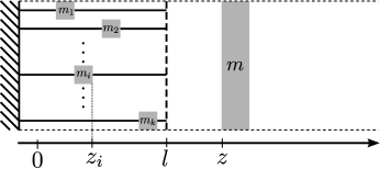
Figure 5.1: In this model, masses $m_{i}$ constitute the wall system, while $m$ is the free mass. The system is essentially one-dimensional.

The positions of the $m_{i}$ are $z_{i}\in[0,l]$ and $z\in[0,\infty)$. Let $M=m+m_{1}+\dots+m_{k}$. In the new coordinates $x_{i}=\sqrt{m_{i}/M}\,z_{i}$, $x_{k+1}=\sqrt{m/M}z$, the kinetic energy form becomes

$$K(x,\dot{x})=({M}/2)\left(\dot{x}_{1}^{2}+\cdots+\dot{x}_{k+1}^{2}\right).$$

We may equivalently assume that $(x_{1},\dots,x_{k})$ defines a point on the torus $\mathbb{T}^{k}$ by taking the range of $x_{i}$ to be $[-a_{i}/2,a_{i}/2]$, where $a_{i}=2\sqrt{m_{i}/M}\,l$, and identifying the end points $a_{i}/2$ and $-a_{i}/2$. Mass $m$ is then constrained to move on the interval defined by

$$x_{k+1}\geq F(x_{1},\dots,x_{k}):=\max\left\{\sqrt{m/m_{1}}\,|x_{1}|,\dots,\sqrt{m/m_{k}}\,|x_{k}|\right\}.$$

Thus the configuration manifold is $M=\left\{(x,x_{k+1})\in\mathbb{T}^{k}\times\mathbb{R}:x_{k+1}\geq F(x)\right\}$, and collision is represented (due to energy and momentum conservation and time-reversibility), by specular reflection at the boundary of $M$ as depicted in Figure 5.2.

This deterministic billiard system can be turned into a random scattering system in several ways. We illustrate two natural possibilities, which we call the heat bath model and the random elastic collision model. The assumptions for the heat bath model are as follows: at the moment $m$ crosses $z=l$ into $[0,l]$, the initial position of each $m_{i}$ is a random variable uniformly distributed over $[0,l]$, and the velocity of $m_{i}$ is normally distributed with mean $0$ and variance $\sigma_{i}^{2}$. We assume that these $\sigma_{i}^{2}$ are such that $m_{i}\sigma_{i}^{2}=m_{j}\sigma_{j}^{2}$ for all $i$ and $j$. In physical terms, we are imposing a condition of equipartition of energy among the wall-bound masses. In the new coordinates $x_{i}$ the velocities are normal random variables with mean $0$ and equal variance $\sigma^{2}=({m_{i}}/{M})\sigma_{i}^{2}$.

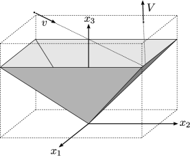
Figure 5.2: Billiard representation of the system of Figure 5.1 for $k=2$.

This is essentially the case described in Corollary 2. The dimensions for the heat bath model are: $n=k=m-1.$ Let $e_{1},\dots,e_{k},e=e_{k+1}$ be the orthonormal basis of coordinate vector fields corresponding to the $x_{i}$. Then the projection to the hyperplane $e^{\perp}$ of the normal vector field $n(x)$ to the graph of $F$ is

$$\overline{n}(x)=\pm\sqrt{\frac{m}{m+m_{i}}}\,e_{i}\text{ for $x$ such that }|x_{i}|\geq\max_{j}|x_{j}|.$$

Therefore, $A$ is the diagonal matrix

$$A=V_{0}\sum_{i=1}^{k}\frac{m}{m+m_{i}}e_{i}^{*}\otimes e_{i}$$

where $V_{0}$ is the volume of the sector $|x_{i}|\geq\max_{j}|x_{j}|$, normalized so that the total volume of the torus is $1$. The matrix $C$ is the covariance matrix of the velocity $\dot{x}$, and is by assumption the scalar matrix $C=\sigma^{2}\sum_{i}e_{i}^{*}\otimes e_{i}$.

Therefore,

$${\text{Tr}\left(CA\right)}/{\text{Tr}(A)}=\sigma^{2},\ \text{Tr}(A)=\sum_{i=1}^{k}\frac{m}{m+m_{i}},\ h=\max_{j}\left\{\frac{m}{m_{1}},\dots,\frac{m}{m_{k}}\right\}.$$

Let us say for concreteness that all the wall-bound masses are equal to $m_{0}$, so $h=m/m_{0}$ and $\Lambda$ becomes the identity matrix times $V_{0}$, whose trace is $kV_{0}$. From Corollary 1 we obtain, for the heat bath model with small ratio $m/m_{0}$ and $k$ equal bound masses, the following differential operator. Let $v$ indicate the velocity of the free mass $m$ (in the new coordinate system, so $v=\dot{x}_{k+1}$) and let $\Phi$ be any compactly supported smooth function on the interval $(0,\infty)$. Then

(5.1) $$\mathcal{L}\Phi=2kV_{0}\sigma^{2}\left[\left(\frac{1}{v}-\frac{v}{\sigma^{2}}\right)\Phi^{\prime}+\Phi^{\prime\prime}\right].$$

The corresponding Itô diffusion has the form

$$dV_{t}=2kV_{0}\sigma^{2}\left(\frac{1}{v}-\frac{v}{\sigma^{2}}\right)\,dt+\sqrt{2kV_{0}\sigma^{2}}\,dB_{t}.$$

Figure 5.3 shows a sample path for this SDE obtained by Euler approximation. (See [12].)

We now consider the random elastic collision model. The assumptions for this model are as follows: the velocities of all the masses $m_{i},m$ constitute the observable variables, and the positions in $[0,l]$ of the wall-bound masses at the moment $m$ crosses into $[0,l]$ are uniformly distributed random variables. This is the case to which Corollary 3 applies, where $n=k$. (The integer $k$ of Theorem 1 is $0$.) Again, for concreteness, suppose that all the wall-bound masses are equal to $m_{0}$. The eigenvalues of $\Lambda=V_{0}I$ are all $\lambda_{i}=V_{0}$. We may assume without loss of generality that the constant speed of the billiard particle (in the billiard representation of Figure 5.2) is $1$ and let $v$ denote the projection of the billiard particle’s velocity to the unit disc $D^{k}_{1}$ in dimension $k$. Then we obtain from Corollary 3:

(5.2) $$(\mathcal{L}\Phi)(v)=2V_{0}\sum_{i=1}^{k}\left(\left(1-|v|^{2}\right)\Phi_{i}\right)_{i}$$

where $\Phi$ is any compactly supported smooth function on $D^{k}_{1}$.

The differential operator of 5.2, as well as 4.5 in Corollary 3, generalize in a natural way the standard Legendre operator defined on functions of the interval $[-1,1]$. We refer to the diffusion process with this type of infinitesimal generator a (generalized) Legendre diffusion. A sample path is shown in Figure 1.3.

It is interesting to notice that the heat bath and random elastic collision models lead to very standard Sturm-Liouville differential operators. For the heat bath, Equation 5.1 is, up to constant, Laguerre’s differential operator. Essentially the same model of heat bath/thermostat described here is used in [4] to build a minimalist mathematical model of a heat engine, described as a random system of billiard type.

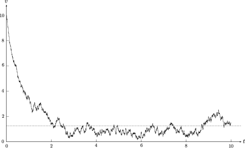
Figure 5.3: A sample path of the Itô equation $dV_{t}=(1/v-v)dt+dB_{t}$. We have used Euler approximation with time length $10$, initial point $v=10$, and number of steps $=10000$. The mean value relative to the stationary distribution is $\sqrt{\pi/2}$, corresponding to the horizontal dashed line.

5.4 Example: collisions of point mass and moving surface

Here we give the differential equation approximation of $P-I$ for the example of Subsection 3.2. The main interest in this example is that it is the simplest that combines the features of the two cases considered above in Subsection 5.3.

It is first necessary to describe the operator $A$ (see Subsection 4.2). The notations are as in that subsection. The torus $\mathbb{T}^{2}$ has fundamental domain (centered at $(0,0)$)

$$|x_{0}|\leq\tau/2,\ \ |x_{1}|\leq 1/2,\ \ \tau=\frac{a_{0}}{a_{1}}\sqrt{\frac{m_{0}}{m_{1}}}.$$

The billiard boundary surface is the graph of $x_{2}=F(x_{0},x_{1})$, where

$$F(x_{0},x_{1})=\sqrt{\frac{m_{1}}{m_{0}}}|x_{0}|+a_{1}^{-1}f(a_{1}x_{1}).$$

Let $e_{0},e_{1},e:=e_{2}$ be the standard coordinate vector fields for the coordinate system $(x_{0},x_{1},x_{2})$. It is easily checked that $A$ is

$$A=\left(\frac{m_{1}}{m_{0}}+O(h^{4})\right)e_{0}^{*}\otimes e_{0}+\left(\int_{0}^{1}[f^{\prime}(a_{1}s)]^{2}\,ds+O(h^{4})\right)e_{1}^{*}\otimes e_{1},$$

where the error term satisfies $0\leq O(h^{2})\leq h^{2}$, while the norm of $A$ satisfies $\|A\|\leq h.$ As an example, take

$$f(z_{1})=\sqrt{R^{2}-z_{1}^{2}}-\sqrt{R^{2}-a_{1}^{2}/4}.$$

The graph of $f$ is an arc of circle of radius $R$ intersecting the $z_{1}$-axis at the points $(\pm a_{1}/2,0)$. Let the scale-free curvature be $\kappa:=a_{1}/R<1$. Then

$$a:=\int_{0}^{1}[f^{\prime}(a_{1}s)]^{2}\,ds={\kappa}^{-1}\ln\frac{1+\frac{\kappa}{2}}{1-\frac{\kappa}{2}}-1=\frac{\kappa^{2}}{12}+O(\kappa^{3}).$$

Thus for small values of $h$ (disregarding terms in $\kappa$ or order greater than $2$, and in $m_{1}/m_{0}$ of order greater than $1$) we have

$$A=\frac{m_{1}}{m_{0}}e_{0}^{*}\otimes e_{0}+\frac{\kappa^{2}}{12}e_{1}^{*}\otimes e_{1}\text{ and }h=\frac{\kappa^{2}}{4}+\frac{m_{1}}{m_{0}}.$$

The operator $C$ takes the form

$$C=\int_{-\infty}^{\infty}w^{2}\,d\mu(w)e_{0}^{*}\otimes e_{0}=\sigma^{2}e_{0}^{*}\otimes e_{0}.$$

We observe that $\text{Tr}(CA)=\frac{m_{1}}{m_{0}}\sigma^{2}$ and $\text{Tr}(A)=\frac{m_{1}}{m_{0}}+a$. For the special case of an arc of circle, $a=\kappa^{2}/12$, where $\kappa$ is the scale free curvature. This yields the approximation, written informally as

(5.3) $$\frac{(P\Phi)(v)-\Phi(v)}{2}\approx\frac{m_{1}}{m_{0}}\sigma^{2}\mathcal{L}_{\text{\tiny temp}}\Phi+\frac{\kappa^{2}}{12}\mathcal{L}_{\text{\tiny curv}}\Phi$$

where

$$\mathcal{L}_{\text{\tiny temp}}\Phi =\left(\frac{1}{v_{2}}-\frac{v_{2}}{\sigma^{2}}\right)\Phi_{2}+\Phi_{22}$$

$$\mathcal{L}_{\text{\tiny curv}}\Phi =-2v_{1}\Phi_{1}+\frac{v_{1}^{2}-v_{2}^{2}}{v_{2}}\Phi_{2}-2v_{1}v_{2}\Phi_{12}+v_{2}^{2}\Phi_{11}+v_{1}^{2}\Phi_{22}$$

The mass-ratio and curvature parameters may a priori go to $0$ independently with $h$ (under Assumption 1) and the particular way in which each goes to $0$ matters for the limit. Expression 5.3 shows that taking $h$ for the denominator in the quotient $(P_{h}\Phi-\Phi)/h$ used in the definition of $\mathcal{L}$ is essentially an arbitrary choice. One could have taken instead $\text{Tr}(A)$, for example. If we further ask in this example that the scale-free curvature and the mass ratio be coupled by a linear relation such as $\frac{m_{1}}{m_{0}}=\alpha\frac{\kappa^{2}}{4}$, for a fixed but arbitrary constant $\alpha>0$, and keep the original choice of denominator $h$, then

$$\Lambda=\lim_{h\rightarrow 0}A/h=\frac{\alpha}{1+\alpha}e_{0}^{*}\otimes e_{0}+\frac{1}{3(1+\alpha)}e_{1}^{*}\otimes e_{1}.$$

This gives the family of operators (depending on $\alpha$)

$$\left(\mathcal{L}\Phi\right)(v)=\lim_{h\rightarrow 0}\frac{(P_{h}\Phi)(v)-\Phi(v)}{h} =\frac{2\sigma^{2}\alpha}{1+\alpha}\left\{\left(\frac{1}{v_{2}}-\frac{v_{2}}{\sigma^{2}}\right)\Phi_{2}+\Phi_{22}\right\}+$$

$$\frac{2}{3(1+\alpha)}\left\{-2v_{1}\Phi_{1}+\frac{v_{1}^{2}-v_{2}^{2}}{v_{2}}\Phi_{2}-2v_{1}v_{2}\Phi_{12}+v_{2}^{2}\Phi_{11}+v_{1}^{2}\Phi_{22}\right\}.$$

In the concrete example of Figure 1.2 we took $\alpha=1$, $\sigma^{2}=1/3$ (and multiply the the operator by an overall factor $3$ to make it look simpler).

The expression 5.3, points to a separation between, on the one hand, the term responsible for the change in speed, which contains the variance (temperature) $\sigma^{2}$ and the mass ratio, and on the other, a purely geometric term that involves the scale free curvature $\kappa$. If we let $\sigma^{2}$ be $0$ and the wall mass $\infty$, and consider $\kappa$ to be small, the MB-Laplacian reduces to $\mathcal{L}_{\text{\tiny curv}}$. It is interesting to note that $\mathcal{L}_{\text{\tiny curv}}|v|^{2}=0$, so the diffusion associated to this second order operator restricts to hemispheres of arbitrary radius, and we have a Legendre diffusion. (See Proposition 5.)

Acknowledgment: Hong-Kun Zhang was partially funded by NSF Grant DMS-090144 and NSF CAREER Grant DMS-1151762.

References

- [1] C. Cercignani and D. H. Sattinger, Scaling Limits and Models in Physical Processes, DMV Seminar Band 28, Birkäuser, 1998.
- [2] F. Celestini and F. Mortessagne, Cosine law at the atomic scale: toward realistic simulations of Knudsen diffusion, Physical Review E 77, 021202 (2008).
- [3] N. Chernov and R. Markarian, Chaotic Billiards, Mathematical Surveys and Monographs, 127, American Mathematical Society, 2006.
- [4] T. Chumley, S. Cook and R. Feres, From billiards to thermodynamics, 2012, arXiv:1207.5878v1
- [5] F. Comets, S. Popov, G. M. Schutz, M. Vachkovskaia, Billiards in a general domain with random reflections. Arch. Ration. Mech. Anal. 191 (2008), 497-537.
- [6] F. Comets, S. Popov, G. M. Schutz, M. Vachkovskaia, Knudsen gas in a finite random tube: transport diffusion and first passage properties, J. Stat. Phys. 140, 948-984 (2010).
- [7] S. Cook and R. Feres, Random billiards with wall temperature and associated Markov chains, Nonlinearity 25 (2012) 2503-2541.
- [8] R. Feres, Random walks derived from billiards, in Dynamics, Ergodic Theory, and Geometry, Ed. Boris Hasselblatt, MSRI Publications, Cambridge University Press, (2007) 179-222.
- [9] R. Feres and H-K. Zhang, The spectrum of the billiard Laplacian of a family of random billiards, Journal of Statistical Physics, V. 141, N. 6 (2010) 1030-1054.
- [10] R. Feres and H-K. Zhang, Spectral Gap for a Class of Random Billiards, Comm. Math. Phys. 313, 479-515, 2012.
- [11] S. Harris, An introduction to the theory of the Boltzmann equation, Dover, 1999.
- [12] P. E. Kloeden and E. Platen, Numerical Solutions of Stochastic Differential Equations, Springer, 1995.
- [13] S. Meyn and R. L. Tweedie, Markov Chains and Stochastic Stability, second edition, Cambridge University Press, 2009.
- [14] B. Oksendal, Stochastic Differential Equations, Springer, 1998.
- [15] D. W. Stroock, S. R. S. Varadhan, Multidimensional Diffusion Processes. Classics in Mathematics, Springer, 2006.