The performance of the quantum adiabatic algorithm
on random instances of two optimization problems on regular hypergraphs
Abstract
In this paper we study the performance of the quantum adiabatic algorithm on random instances of two combinatorial optimization problems, 3-regular 3-XORSAT and 3-regular Max-Cut. The cost functions associated with these two clause-based optimization problems are similar as they are both defined on 3-regular hypergraphs. For 3-regular 3-XORSAT the clauses contain three variables and for 3-regular Max-Cut the clauses contain two variables. The quantum adiabatic algorithms we study for these two problems use interpolating Hamiltonians which are stoquastic and therefore amenable to sign-problem free quantum Monte Carlo and quantum cavity methods. Using these techniques we find that the quantum adiabatic algorithm fails to solve either of these problems efficiently, although for different reasons.
pacs:
03.67.Ac,05.30.Rt,75.10.Jm,75.50.LkI Introduction
The Quantum Adiabatic Algorithm (QAA) Farhi et al. (2001) is an algorithm for solving optimization problems using a quantum computer. The optimization problem to be solved is defined by a cost function which acts on bit strings. The computational task is to find the global minimum of the cost function.
To use the QAA, the cost function is first encoded in a quantum Hamiltonian (called the ‘problem Hamiltonian’) that acts on the Hilbert space of spin particles. The problem Hamiltonian is written as a function of Pauli-matrices and is therefore diagonal in the computational basis. The ground state of corresponds to the solution (i.e., lowest cost bit string) of the optimization problem.
To find the ground state of the problem Hamiltonian, the system is first prepared in the ground state of another Hamiltonian , known as the beginning Hamiltonian. The beginning Hamiltonian does not commute with the problem Hamiltonian and must be chosen so that its ground state is easy to prepare. Here we use the standard choice
which has a product state as its ground state.
The Hamiltonian of the system is slowly modified from to . Here we consider a linear interpolation between the two Hamiltonians
| (1) |
where is a parameter varying smoothly with time, from to at the end of the algorithm after a total evolution time .
If the parameter is changed slowly enough, the adiabatic theorem of Quantum Mechanics Kato (1951); Messiah (1962); Amin (2009); Jansen et al. (2007)), ensures that the system will stay close to the ground state of the instantaneous Hamiltonian throughout the evolution. After time the state obtained will be close to the ground state of . A final measurement of the state in the Pauli- basis then produces the solution of the optimization problem.
The runtime must be chosen to be large enough so that the adiabatic approximation holds: this condition determines the efficiency, or complexity, of the QAA. A condition on can be given in terms of the eigenstates and eigenvalues of the Hamiltonian , as Wannier (1965); Farhi et al. (2002)
| (2) |
where is the minimum of the first excitation gap with , and .
Typically, matrix elements of scale as a low polynomial of the system size , and the question of whether the runtime is polynomial or exponential as a function of therefore depends on how the minimum gap scales with . If the gap becomes exponentially small at any point in the evolution, then the computation requires an exponential amount of time and the QAA is inefficient. The dependence of the minimum gap on the system size for a given problem is therefore a central issue in determining the complexity of the QAA.
A notable feature of the interpolating Hamiltonian (1) is that it is real and all of its off diagonal matrix elements are non-positive. Hamiltonians which have this property are called stoquastic Bravyi et al. (2008). There is complexity-theoretic evidence that some computational problems regarding the ground states of stoquastic Hamiltonians are easier than the corresponding problems for more general Hamiltonians Bravyi and Terhal (2009). It may be the case that quantum adiabatic algorithms using stoquastic interpolating Hamiltonians (such as the ones we consider here) are no more powerful than classical algorithms–this remains an intriguing open question.
An interesting question about the QAA is how it performs on “hard” sets of problems – those for which all known algorithms take an exponential amount of time. While early studies of the QAA done on small systems () Farhi et al. (2001); Hogg (2003) indicated that the time required to solve one such problem might scale polynomially with , several later studies using larger system sizes gave evidence that this may not be the case.
References Farhi et al. (2002, 2008) show that adiabatic algorithms will fail if the initial Hamiltonian is chosen poorly. Recent work has elucidated a more subtle way in which the adiabatic algorithm can fail Altshuler et al. (2010); Amin and Choi (2009); Farhi et al. (2011); Altshuler et al. (2009); Foini et al. (2010). The idea of these works is that a very small gap can appear in the spectrum of the interpolating Hamiltonian due to an avoided crossing between the ground state and another level corresponding to a local minimum of the optimization problem. The location of these avoided crossings moves towards as the system size grows. They have been called “perturbative crosses” because it is possible to locate them using low order perturbation theory. Altshuler et al. Altshuler et al. (2009) have argued that this failure mode dooms the QAA for random instances of NP-complete problems. However, the arguments of Altshuler et al. have been criticized by Knysh and Smelyanskiy Knysh and Smelyanskiy (2011). The application of the QAA to hard optimization problems has been reviewed recently in Ref. Bapst et al. (2012).
Young et al. Young et al. (2008, 2010) recently examined the performance of the QAA on random instances of the constraint satisfaction problem called 1-in-3 SAT (to be described in the next section) and showed the presence of avoided crossings associated with very small gaps. These ‘bottlenecks’ appears in a larger and larger fraction of the instances as the problem size increases, indicating the existence of a first order quantum phase transition. This leads to an exponentially small gap for a typical instance, and therefore also to the failure of adiabatic quantum optimization.
It is not yet clear to what extent the above behavior found for 1-in-3 SAT is general and whether it is a feature inherent to the QAA that will plague most if not all problems fed into the algorithm or something more benign than this. Previous work Jörg et al. (2008, 2010a, 2010b); Hen and Young (2011) had argued that a first order quantum phase transition occurs for a broad class of random optimization models.
In this paper we contrast the performance of the quantum adiabatic algorithm on random instances of two combinatorial optimization problems. The first problem we consider is 3-XORSAT on a random 3-regular hypergraph, which was studied previously in Ref. Jörg et al. (2010a). Interestingly, although this computational problem is classically easy–an instance can always be solved in polynomial time on a classical computer by using Gaussian elimination–it is known that classical algorithms that do not use linear algebra are stymied by this problem Franz et al. (2001); Haanpää et al. (2006); Ricci-Tersenghi (2011); Guidetti and Young (2011). In Ref. Jörg et al. (2010a) it was shown that the QAA fails to solve this problem in polynomial time. In this paper we provide more numerical evidence for this. We also furnish a duality transformation that helps to understand properties of this model.
The second computational problem we consider is Max-Cut on a 3-regular graph. This problem is NP-hard. However we consider random instances, for which the computational complexity is less well understood.
A nice feature of these problems is that the regularity of the associated hypergraphs constrains the two ensembles of random instances. Studying the performance of the QAA for these problems, we therefore expect to see smaller instance-to-instance differences than for the unconstrained ensembles of instances.
We use two different methods to study the performance of the QAA. The first method is quantum Monte Carlo simulation. It is a numerical method that is based on sampling paths from the Taylor expansion of the partition function of the system. Using this method we can extract, for a given instance, the thermodynamic properties (in particular the ground state energy) as well as the eigenvalue gap for the interpolating Hamiltonian . This allows us to investigate the size dependence of the typical minimum gap of the problem from which we can extrapolate the large-size scaling of the computation time of the QAA. The second approach is a quantum cavity method. It is a semi-analytical method that allows us to compute the thermodynamic properties averaged over the ensemble of instances in the limit . It leads to a set of self-consistent equations that can be solved analytically in some classical examples Mézard and Parisi (2001, 2003). However in the quantum case the equations are more complicated and are solved numerically Laumann et al. (2008); Krzakala et al. (2008). The method is not exact on general graphs. For locally tree-like random graphs, it provides the exact solution of the problem if some assumptions on the Gibbs measure are satisfied Mézard and Parisi (2001, 2003); Mézard and Montanari (2009). As we will discuss below the cavity method we use in this paper gives the exact result for 3-XORSAT, while it only gives an approximation for the Max-Cut problem.
Using these methods we conclude that the quantum adiabatic algorithm fails to solve both problems efficiently, although in a qualitatively different way.
The plan of this paper is as follows. In Section II we describe the two computational problems that we investigate. In Sec. III we discuss the methods that we use to obtain our results. These results are presented in Sec. IV and our conclusions are summarized in Sec. V. Some parts of this paper have previously appeared in the PhD thesis of one of the authors Gosset (2011).
II Models
We now discuss in detail the two computational problems 3-regular 3-XORSAT and 3-regular Max-Cut.
When studying the efficiency of the QAA numerically Farhi et al. (2001); Young et al. (2008, 2010), it is convenient to consider instances with a unique satisfying assignment (USA) for reasons that will be explained in Sec. III.1. On the other hand, the quantum cavity method is designed to study the ensemble of random instances with no restrictions on the number of satisfying assignments. In this section we specify the random ensembles of instances that we investigate in this paper.
II.1 3-regular 3-XORSAT
The 3-XORSAT problem is a clause based constraint satisfaction problem. An instance of such a constraint satisfaction problem is specified as a list of logical conditions (clauses) on a set of binary variables. The problem is to determine whether there is an assignment to bits which satisfies all clauses.
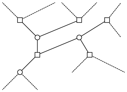
In the 3-XORSAT problem each clause involves three bits. A given clause is satisfied if the sum of the three bits (mod 2) is a specified value (either 0 or 1, depending on the clause). We consider the “3-regular” case where every bit is in exactly three clauses which implies . This model has already been considered by Jörg et al. Jörg et al. (2010a). The factor graph for an instance of 3-regular 3-XORSAT is sketched in Fig. 1.
Since this problem just involves linear constraints (mod 2), the satisfiability problem can be solved in polynomial time using Gaussian elimination. However, it is well known that this problem presents difficulties for solvers that do not use linear algebra (see, e.g. Refs. Franz et al. (2001); Haanpää et al. (2006); Ricci-Tersenghi (2011); Guidetti and Young (2011)).
We associate each instance of 3-regular 3-XORSAT with a problem Hamiltonian that acts on spins. Each clause is mapped to an operator which acts nontrivially on the spins involved in the clause. The operator for a given clause has energy zero if the clause is satisfied and energy equal to if it is not, so
| (3) |
Here each clause is associated with the 3 bits and a coupling which tells us if the sum of the bits mod 2 should be or when the clause is satisfied.
II.1.1 Random Instances of 3-regular 3-XORSAT
As in Ref. Jörg et al. (2010a), we consider both the random ensemble of instances of this problem and the random ensemble of instances which have a unique satisfying assignment (USA). In the 3-XORSAT problem as , instances with a USA are a nonzero fraction, about 0.285 Jörg et al. (2010a), of the set of all instances, so the random ensemble of USA instances should be a good representation of the fully random ensemble.
All satisfiable instances (and in particular instances with a USA) have the property that the cost function Eq. (3) can be mapped unitarily into the form
| (4) |
by a product of bit flip operators.
II.1.2 Previous Work
Reference Jörg et al. (2010a) studied the performance of the QAA on the random ensemble of instances of 3-regular 3-XORSAT using quantum cavity method and quantum Monte Carlo simulation. They also studied the ensemble of random instances with a USA using exact numerical diagonalization. This work gave evidence that there is a first order quantum phase transition which occurs at in the ground state. Their results also demonstrate that the minimum gap is exponentially small as a function of at the transition point.
II.1.3 Duality Transformation
In this section we demonstrate a duality mapping for the ensemble of random instances of 3-regular 3-XORSAT with a unique satisfying assignment. This duality mapping explains the critical value of the quantum phase transition in this model Jörg et al. (2010a). Consider the Hamiltonian
| (5) |
Here, the first term is the beginning Hamiltonian and the second term is the problem Hamiltonian for an instance of 3-regular 3-XORSAT with a unique satisfying assignment. The 3-regular hypergraph specifying the instance can be represented by a matrix where
and where has 3 ones in each row and 3 ones in each column. The fact that there is a unique satisfying assignment is equivalent to the statement that the matrix is invertible over . To see this, consider the equation (with addition mod 2)
This equation has the unique solution if and only if there is a unique satisfying assignment for the given instance. This is also the criterion for the matrix to be invertible.
The duality that we construct shows that the spectrum of is the same as the spectrum of where is obtained by replacing the problem Hamiltonian hypergraph by its dual–that is to say, the instance corresponding to a matrix is mapped to the instance associated with . The ground state energy per spin (averaged over all 3-regular instances with a unique satisfying assignment) is symmetric about and the first order phase transition observed in Ref. Jörg et al. (2010a) occurs at . For each define the operator
| (6) |
We also define, for each clause , a bit string
Here is the unit vector with components . Note that is the unique bit string which violates clause and satisfies all other clauses. Such a bit string is guaranteed to exist since is invertible. Let denote the th bit of the string Define, for each ,
| (7) |
Note that
and
For each bit let be the clauses which bit participates in. Then
| (8) |
This follows from the fact that
and so
The above equation and the definition Eq. (7) show Eq. (8). Now using Eqs. (8) and (6) write
| (9) | |||||
| (10) | |||||
| (11) | |||||
| (12) |
The and operators satisfy the same commutation relations as the operators and . Comparing Eq. (12) with Eq. (5) we conclude that the spectrum of is the same as the spectrum of . This result can be thought of as an extension of the duality of the one-dimensional random Ising model in a transverse field, see e.g. Ref. Fisher (1995).
In Fig. 2 we show the first four energy levels of the interpolating Hamiltonian as a function of for one 16-bit instance of 3-XORSAT. The duality transformation means that these energy levels are the same as for the interpolating Hamiltonian which involves the dual instance. Evident from the figure is the apparent symmetry of the energy levels around . In this case the instance and its dual are similar from the point of view of the QAA.
The duality argument given here has implications for the phase transition which occurs in the ensemble of random instances of 3-regular 3-XORSAT as . Our numerics in section IV show that for large , the ground state energy per spin as a function of (averaged over the ensemble of instances) has a nonzero derivative as . The duality transformation given here implies that this curve is symmetric about . So there is a discontinuity in the derivative of this curve at , which is associated with a first order phase transition.

II.2 3-regular Max-Cut
The second model we discuss is also a clause based problem. The instances we consider are not satisfiable and we are interested in finding the assignment which gives the maximum number of satisfied clauses. We view this problem as minimizing a cost function that computes the number of unsatisfied clauses. The 3-regular Max-Cut problem is defined on bits, and each bit appears in exactly three clauses. Each clause involves two bits and is satisfied if and only if the sum of the two bits (modulo 2) is 1. The number of clauses is therefore . The problem Hamiltonian is
| (13) |
The ground state of this Hamiltonian encodes the solution to the Max-Cut problem.
The model can also be viewed as an antiferromagnet on a 3-regular random graph. Because the random graph in general has loops of odd length, it is not possible to satisfy all of the clauses.
The Max-Cut problem is NP-hard and accordingly there is no known classical polynomial time algorithm which computes the ground state energy of the problem Hamiltonian (13). Indeed, even achieving a certain approximation to the ground state energy is hard, which follows from the fact that it is NP hard to approximate the Max-Cut of -regular graphs to within a multiplicative factor Berman and Karpinski (1999). Interestingly, however, there is a classical polynomial time algorithm which achieves an approximation ratio of at least Halperin et al. (2004).
II.2.1 Random Instances of 3-regular Max-Cut
Using the quantum cavity method we study the ensemble of random instances of 3-regular Max-Cut.
The random instances we studied using quantum Monte Carlo simulation were restricted to those which have exactly 2 minimal energy states (note that this is the smallest number possible since the problem is symmetric under flipping all the spins) and for which the ground state energy of the problem Hamiltonian is equal to . We choose to study instances with a unique satisfying assignment (up to the bit-flip symmetry of this problem) because it is numerically more convenient for the extraction of the relevant gap (to the first even state). For the range of sizes studied, was found numerically to be the most probable value of the ground state energy. The restriction to instances with a fixed Max-Cut () further reduces the instance-to-instance fluctuations. However, this choice affects the ensemble averaged value of thermodynamic observables (e.g. the average energy of fully random instances is different from ), making it more difficult to compare the quantum Monte Carlo results with our quantum-cavity results on the fully random ensemble. We expect (and find numerically) that this set of instances makes up an exponentially small fraction of the whole random ensemble for large .
II.2.2 Previous work
Laumann et al. Laumann et al. (2008) used the quantum cavity method to study the transverse field spin glass with the problem Hamiltonian
| (14) |
where each is chosen to be or with equal probability.
In general there is no “gauge transformation” equivalence between this problem Hamiltonian and the antiferromagnetic problem Hamiltonian Eq. (13). However we do expect these models to exhibit similar properties since a random graph is locally tree-like, and on a tree such a gauge transformation does exist, see Ref. Zdeborová and Boettcher (2010) for a discussion of this point in the case where there is no transverse field present.
Laumann et al. found that this system exhibits a second order phase transition as a function of the transverse field. Their method is similar to the quantum cavity method that we use, although the numerics performed in Ref. Laumann et al. (2008) have some systematic errors which our calculations avoid. The method used in Ref. Laumann et al. (2008) is a discrete imaginary time formulation of the quantum cavity method which has nonzero Trotter error, whereas our calculation works in continuous imaginary time Krzakala et al. (2008) where this source of error is absent. Our calculation also does not use the approximation used in Ref. Laumann et al. (2008) where the “effective action” of a path in imaginary time is truncated at second order in a cluster expansion.
III Method
III.1 Quantum Monte Carlo
The complexity of the QAA algorithm is determined by the size dependence of the “typical” minimum gap of the problem. Following Refs. Young et al. (2008, 2010); Hen and Young (2011), we analyze the size-dependence of these gaps by considering (typically) 50 instances for each size, and then extracting the minimum gap for each of them. For each instance, we perform quantum Monte Carlo simulations for a range of values and hunt for the minimum gap. We then take the median value of the minimum gap among the different instances for a given size to obtain the “typical” minimum gap. In situations where the distribution of minimum gaps is very broad, the average can be dominated by rare instances which have a much bigger gap than the typical one, and so the typical value (characterized, for example, by the median) is a better measure than the average. This has been discussed in detail by Fisher Fisher (1995) who solved the random transverse field model in one-dimension exactly, and found that the average gap at the quantum critical point vanishes polynomially with while the typical gap has stretched exponential behavior, .
Quantum Monte Carlo simulation works by sampling random variables from a probability distribution (over some configuration space) which contains information about the quantum system of interest. The probability distribution is sampled by Markov chain Monte Carlo, and properties of the quantum system to be studied are obtained as expectation values. Different quantum Monte Carlo methods are based on different ways of associating probability distributions to a quantum system.
In our simulations we use a quantum Monte Carlo technique known as the stochastic series expansion (SSE) algorithm Sandvik (1999, 1992). In this method, the probability distribution associated with the quantum system is derived from the Taylor series expansion of the partition function at inverse temperature . This is in contrast to other quantum Monte Carlo techniques which are based on the path integral expansion of the partition function. Whereas some of these techniques have systematic errors because the path integral expansions used are inexact, the SSE that we use has no such systematic error.
A second feature of the SSE method that we use is that the Markov chain used to sample configurations allows global, as well as local, updates, which leads to faster equilibration. We further speed up equilibration by implementing “parallel tempering” Hukushima and Nemoto (1996), where simulations for different values of are run in parallel and spin configurations with adjacent values of are swapped with a probability satisfying the detailed balance condition. Traditionally, parallel tempering is performed for systems at different temperatures, but here the parameter plays the role of (inverse) temperature Sengupta et al. (2002).
The details of our implementations of the SSE method for 3-XORSAT and Max-Cut are slightly different and are further discussed in Appendix A. Moreover, the Max-Cut problem can not be simulated with the ‘traditional’ SSE method because of its symmetry under flipping all of the spins: For a given instance of Max-Cut, every eigenstate of the interpolating Hamiltonian is either even or odd under this symmetry transformation. Since the ground state is even, here we are interested in the eigenvalue gap to the first even excited state. We therefore design our quantum Monte Carlo simulation so that it works in the subspace of even states. The modified algorithm is detailed in Appendix B.
In our simulations we extract the gap from imaginary time-dependent correlation functions. The gap of the system for a given instance and a given value is extracted by analyzing measurements of (imaginary) time-dependent correlation functions of the type
| (15) |
where the operator is some measurable physical quantity. It is useful to optimize the choice of correlation functions such that the contribution from the first excited state, in Eq. (16) below, is as large as possible relative to the contributions from higher excited states. One way of doing this, which was used in some of the runs, is described in Ref. Hen (2012).
The evaluation of in the above equation is computed from the product where the two indices correspond to different independent simulations of the same system. This eliminates the bias stemming from straightforward squaring of the expectation value.
In the low temperature limit, where , the system is in its ground state so the imaginary-time correlation function is given by
| (16) |
where . At long times, , the correlation function is dominated by the smallest gap (as long as the matrix element is nonzero). On a log-linear plot , then has a region where it is a straight line whose slope is the negative of the gap. This can therefore be extracted by linear fitting. A more detailed description of the method may be found in Ref. Hen (2012).
III.2 The quantum cavity method
The quantum cavity method Krzakala et al. (2008); Laumann et al. (2008) is a technique that is used to study thermodynamic properties of transverse field spin Hamiltonians. In our implementation we use the continuous imaginary time method from Ref. Krzakala et al. (2008). Quantum Cavity methods have now been used to study a number of problems including the ferromagnet on the Bethe lattice in uniform Krzakala et al. (2008) and random Dimitrova and Mezard (2011) transverse field, the spin glass on the Bethe Lattice Laumann et al. (2008), 3-regular 3-XORSAT Jörg et al. (2010a), and the quantum Biroli-Mézard model Foini et al. (2011).
If the Hamiltonian is a two-local transverse field Hamiltonian on a finite number of spins and if the interaction graph consists of a tree (i.e if there are no loops) then the quantum cavity equations are exact. In this case the quantum cavity equations are a closed set of equations that exactly characterize the thermodynamic properties of the system at a fixed inverse temperature . If instead the interaction graph is a random regular graph with a finite number of spins then it must have loops. As we can think of it as an “infinite tree” since the typical size of loops in such a graph diverges.
Quantum cavity methods (such as the one we use) for problems defined on random regular graphs make use of two properties of the system: (i) the fact that a random regular graph is locally tree-like; (ii) the fact that spin-spin correlations decay quickly as a function of distance. While the first property is true with probability 1 for random regular graphs when , the second property is not always true and we now discuss it more carefully.
The simplest case is when the Gibbs measure is characterized by a single pure state that has the clustering property, as in a paramagnetic phase. This happens at high enough temperature or large enough transverse field. In this case, correlations decay exponentially and the simplest version of the cavity method (the so-called “replica symmetric (RS)” cavity method) gives the exact result. Upon lowering the temperature or the transverse field, a phase transition towards a more complicated phase can be encountered. If this phase is a standard broken-symmetry phase (e.g. a ferromagnetic phase), then correlation decay holds provided one adds an infinitesimal symmetry-breaking field, and the RS cavity method still provides the exact result Krzakala et al. (2008).
However, if the transition is to a spin glass phase, then the Gibbs measure is split into a large number of states, and the decorrelation property that is required by the cavity method only holds within each state. In this case, there is no explicit symmetry breaking, therefore the states cannot be selected by adding an infinitesimal external field. It turns out that refined versions of the cavity method must be used, that are based on assumptions on the structure of these states Mézard and Montanari (2009). The simplest assumption is that states are distributed in a uniform way in the phase space of the system, and leads to the so-called “1 step replica symmetry breaking (1RSB)” approximation. In more complicated cases, states might be arranged in “clusters” leading to a hierarchical organization, and this requires further steps of RSB Mézard et al. (1987). A consistency check can be performed within the method to check whether a given RSB scheme gives the exact result or whether further RSB steps are required.
For the XORSAT problem on random regular graphs, it can be rigorously shown that the 1RSB scheme gives the exact result in the classical case Mézard et al. (2003); Cocco et al. (2003), and it has been conjectured that the same is true for the quantum problem in transverse field Jörg et al. (2010a). For the specific case of 3-regular 3-XORSAT investigated here, a RS calculation is enough to get the thermodynamic properties Jörg et al. (2010a), which is why we use the RS method in our simulations of this model. We study this problem at a temperature low enough that no residual temperature dependence of the energy is observed. Furthermore, we set the parameters of our calculation to be more computationally demanding than those of reference Jörg et al. (2010a), which allows us to achieve better precision.
The study of 3-regular Max-Cut is more involved. To understand how well the cavity method works on this problem, we can look at results obtained for the classical 3 regular spin-glass with Hamiltonian (14). We expect that these problems have very similar (possibly identical) thermodynamic properties Zdeborová and Boettcher (2010). For the classical 3-regular spin glass it can be shown that neither the RS nor the 1RSB cavity method give exact results Mézard and Parisi (2001, 2003); Zdeborová and Boettcher (2010), and it is widely believed that an infinite number of RSB steps is required (this has been shown rigorously for the -regular spin glass as , which corresponds to the Sherrington-Kirkpatrick model Mézard et al. (1987)). However the 1RSB calculation gives a good approximation to the classical ground state energy Mézard and Parisi (2003).
To study 3-regular Max-Cut we used the 1RSB quantum cavity method with Parisi parameter . This level of approximation is more accurate than the replica symmetric approximation but less accurate than the full 1RSB calculation. With this method we studied the limit of the random ensemble of 3-regular Max-Cut Hamiltonians
We ran our calculations at finite inverse temperature and various values of the transverse field . Thermodynamic expectation values with respect to at inverse temperature can be related to thermodynamic expectation values with respect to at and inverse temperature . Note that there is an dependence introduced in the temperature when relating these two thermodynamic ensembles.
IV Results
In what follows we present the results of the QMC simulation alongside those of the quantum cavity results for the two problems we study here. We show that the QAA fails with the choice of interpolating Hamiltonians discussed previously; for both problems the running time appears to be exponentially long as a function of the problem size. However, the reasons for this failure are different for each of the models.
IV.1 Random 3-regular 3-XORSAT
The 3-regular 3-XORSAT problem was studied by Jörg et al. Jörg et al. (2010a) who determined the minimum gap for sizes up to . Here, we extend the range of sizes up to by quantum Monte Carlo simulations. The two sets of results agree and provide compelling evidence for an exponential minimum gap. The duality argument in Sec. II.1.3, shows that the quantum phase transition occurs exactly at . Our numerics show that the phase transition is strongly first order, in agreement with Ref. Jörg et al. (2010a).

We show results for the median minimum gap as a function of size for the 3-regular 3-XORSAT problem in Fig. 3 (log-lin). A straight line fit works well for the log-lin plot, which provides evidence that the minimum gap is exponentially small in the system size. The results shown here generalize and agree with those obtained by Jörg et al. Jörg et al. (2010a). While Ref. Jörg et al. (2010a) computed the average minimum gap and we computed the median, the difference here is very small because the distribution of minimum gaps is narrow for this problem, see for example Fig. 21 of Ref. Bapst et al. (2012).
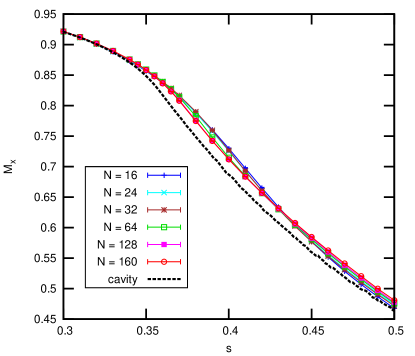
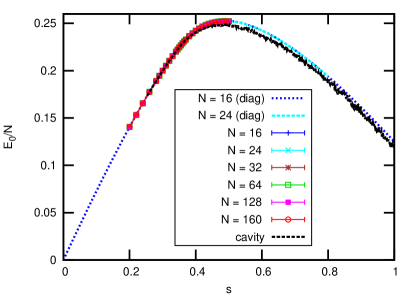
We also computed some ground-state properties of the model: the energy , the magnetization along the -axis , and the spin-glass order parameter defined by:
| (17) |
These quantities, averaged over 50 instances for each size, are plotted in Figs. 4, 5, and 6.

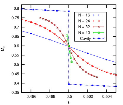

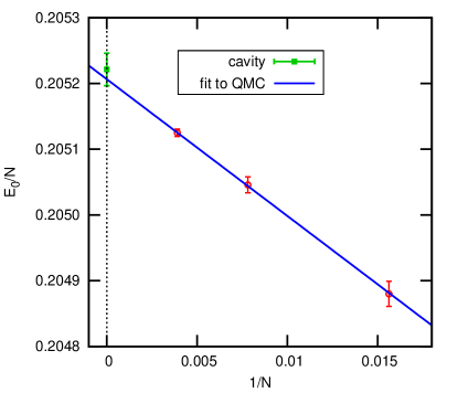
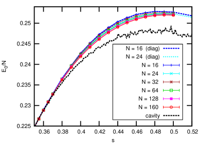
Figure 4 shows that for large system sizes differences between the QMC results for the ground state energy and the (replica symmetric) cavity results are small. Reference Jörg et al. (2010a) has argued that the replica symmetric (RS) cavity method is actually exact for the thermodynamic properties of the 3 regular 3-XORSAT problem. To check this, in Fig. 7 we have expanded the vertical scale and show an extrapolation of the QMC results to at the critical value (where finite-size corrections are largest). The extrapolated value appears to be consistent with the cavity result.
The rapid variation of and shown in figures 5 and 6 in the vicinity of is evidence for a first-order transition. Figure 5 also shows a discontinuity in the -axis magnetization predicted by the cavity calculations at . In the quantum Monte Carlo data we see that the slope of the magnetization increases with and is therefore consistent with the cavity prediction for .
IV.2 Random 3-regular Max-Cut
In the Monte Carlo simulations of the Max-Cut problem we restrict ourselves to instances for which the problem Hamiltonian has a ground state degeneracy of two, and for which the ground state energy is . For this ensemble of instances, we measured the energy, the -magnetization and the spin-glass order parameter using quantum Monte Carlo simulations. Because of the bit-flip symmetry of the model, we use the following different definition of the spin glass order parameter:
| (18) |
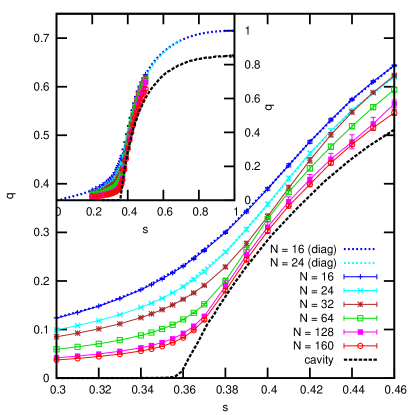
In Figs. 8, 9 and 10 we compare the QMC results with those of our quantum cavity method computation. Recall that the cavity method results apply to the random ensemble of instances. Formally the value of the spin glass parameter from Eq. (17) is zero due to the bit flip symmetry of the Hamiltonian. However, the cavity method works in the thermodynamic limit in which this symmetry is spontaneously broken for greater than the critical value . For the cavity calculations, we measure a spin glass order parameter which is the magnetization squared for each thermodynamic “state”, averaged over the states. This becomes non-zero for as shown in Fig. 8. The Monte Carlo results are consistent with this value of . The inset of Fig. 8 shows a global view of the two spin glass order parameters that we measure, over the whole range of . There we see differences between the (different) order parameters measured using Monte Carlo and cavity calculations for large . Note that the Monte Carlo simulations take only instances with a doubly degenerate ground state for the problem Hamiltonian, , so in this limit, whereas the cavity calculations are done for the random ensemble where the instances have much larger degeneracy at and so in this limit.
Our numerical results for the -component of the magnetization are shown in Fig. 9. We see no evidence of a discontinuity in this quantity at for large . This is in contrast with the corresponding plot for 3-XORSAT in figure 5.
Results for the energy of the Max-Cut problem, obtained both from Monte Carlo and the cavity approach are shown in Fig. 10. The two agree reasonably well but there are differences in the spin glass phase, , which may be due to the different ensembles used in the two calculations. We also note that our cavity method computation is performed at nonzero temperature.
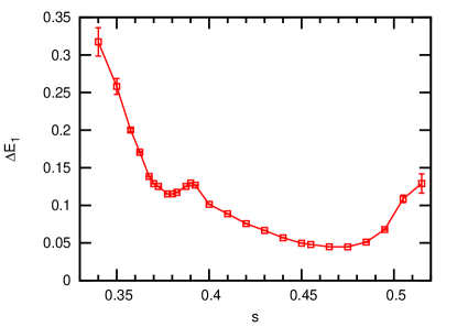
Using quantum Monte Carlo simulations we have determined the energy gap as a function of for in the range between (i.e. well below ) and (i.e. well above ) for sizes between and . For the smaller sizes we find a single minimum in this range, which lies a little above . However, for larger sizes, we see a fraction of instances in which there is a minimum close to and a second, deeper, minimum for well inside the spin-glass phase. A set of data which shows two minima is presented in Fig. 11. This interesting behavior of the minimum gaps suggests the following interpretation: The minima found close (just above) correspond to the order-disorder quantum phase transition. Above the system is the spin-glass phase. The minima that are well within the spin-glass phase may correspond to ‘accidental’ or perturbative crossings in the spin glass.
Double-minima occurrences become more frequent as the system size increases. While no double minima were found for sizes and (within the studied range of values), for sizes and the percentage of instances that exhibit such double minima was found to be approximately , and , respectively (obtained from instances for each size).
We have therefore performed two analyses on the data for the gap. In the first analysis we determine the global minimum (for the range of studied) for each instance and determine the median over the instances. There are about 50 instances for each size. This data is presented in Table 1, and is plotted in Fig. 12 both as log-lin (main figure) and log-log (inset). A straight line fit works well for the log-lin plot (goodness of fit parameter ), provided that we omit the two smallest sizes. The goodness of fit parameter is the probability that, given the fit, the data could have the observed value of or greater, see Ref. Press et al. (1992). However, a straight-line fit works much less well for the log-log plot (), again omitting the two smallest sizes, because the data for the largest size lies below the extrapolation from smaller sizes. If smaller points do not lie on the fit, it is possible that the fit is correct and the deviations are due to corrections to scaling. However, if the largest size shows a clear deviation then the fit can not describe the asymptotic large- behavior. From these fits we conclude that an exponentially decreasing gap is preferred over a polynomial gap.
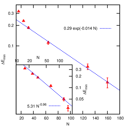
| N | Median gap | Error |
|---|---|---|
| 16 | 0.3203 | 0.0056 |
| 24 | 0.2323 | 0.0057 |
| 32 | 0.1844 | 0.0057 |
| 64 | 0.1113 | 0.0058 |
| 128 | 0.0496 | 0.00473 |
| 160 | 0.0291 | 0.0049 |
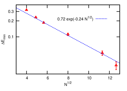
There are other possibilities for the scaling of the minimum gap with size, in addition to polynomial or exponential. For example, we considered a “stretched exponential” scaling of the form . Omitting the first two points (as we did for the exponential fit) we find the fit is satisfactory, as shown in the upper panel of Fig. 13 (). Hence it is possible that the minimum gap decreases as a stretched exponential.
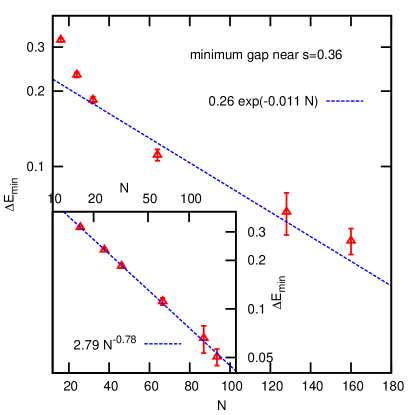
However, if for the instances with more than one minimum, we just take the minimum close to the critical value , a different picture emerges, as shown in Fig. 14. In this case, a straight line fit works well for the log-log plot (), but poorly for the log-lin plot (). For consistency, we again omitted the two smallest sizes for the log-lin plot. These results indicate that the gap only decreases polynomially with size near the quantum critical point.
So far we have plotted results for the median minimum gap, which is a measure of the typical value. However, it is important to note that there are large fluctuations in the value of the minimum gap between instances. This is illustrated in Fig. 15 which presents the values of the minimum gap for all 47 instances for . For the 19 instances with two minima in the range of studied, the minimum at larger is lower than the one at smaller . For these instances, the figure shows both the “local” (smaller-), and the “global” (larger-) minima.
From Fig. 15 we note that a substantial fraction of instances for N = 160 have a minimum gap which is much smaller than the median, . Smaller sizes do not have such a pronounced tail in the distribution for small gaps. We should mention that the gap is not precisely determined if it is extremely small because we require the condition . For we took so this condition is well satisfied for gaps around the median. Hence we are confident that the median is accurately determined. However, it is not well satisfied for the smallest gaps in Fig. 15. Thus, while it is clear that a non-negligible fraction of instances for do have a very small minimum gap, the precise value of the very small gaps in Fig. 15 is uncertain. We note that if the fraction of instances with a very small minimum gap continues to increase with , then, asymptotically, the median would decrease faster than that shown by the fit in the main part of Fig. 12.

V Summary and conclusions
It was demonstrated in Ref. Jörg et al. (2010a) that the quantum adiabatic algorithm fails to solve random instances of 3-regular 3-XORSAT in polynomial time, due to an exponentially small gap in the interpolating Hamiltonian which occurs near . This exponentially small gap is associated with a first order quantum phase transition in the ground state. In this work we have provided additional numerical evidence for this. We have also demonstrated using a duality transformation that the critical value of the parameter is in fact at exactly . We have also shown that the ground state energy of the three regular 3-XORSAT model with a transverse field agrees very well with a replica symmetric (RS) cavity calculation. This provides support for the claim of Ref. Jörg et al. (2010a) that the RS calculation is exact for the thermodynamic properties of this model.
For the random ensemble of Max-Cut instances that we consider, we find that the interpolating Hamiltonians exhibit a second order, continuous phase transition at a critical value . Near this critical value of we find that the eigenvalue gaps decrease only polynomially with the number of bits. However, we also observe very small gaps at values , i.e. in the spin glass phase. An analysis of the fits indicates that a gap decreasing exponentially with size is preferred over a polynomially varying gap, though a stretched exponential fit is also satisfactory.
For both of the problems we studied, the adiabatic interpolating Hamiltonians are stoquastic. This makes it possible for us to numerically investigate the performance of the QAA using quantum Monte Carlo simulation and the quantum cavity method. However it is possible that quantum adiabatic algorithms with stoquastic interpolating Hamiltonians are strictly less powerful than more general quantum adiabatic algorithms.
The QMC calculations consider only instances in which the problem Hamiltonian, , has a doubly degenerate ground state and a specified value of the ground state energy. These instances are exponentially rare. By contrast the cavity approach considers random instances. However, we do not think that these restrictions invalidate the conclusions on the minimum gap summarized in the previous paragraph.
Also, it should be noted that inside the spin-glass phase, QMC techniques become less and less efficient as the adiabatic parameter approaches , i.e. when the Hamiltonian approaches the classical problem Hamiltonian. Hence we have not been able to study values much larger than 0.5 for a broad range of sizes. It is possible, indeed likely, that there are other avoided crossings in this range which might lead to even smaller minima than those found in the studied range, . These minima will however not alter the conclusion that the overall scaling of the running time of the QAA – when applied to the Max-Cut problem – appears to grow exponentially (or perhaps in a stretched exponential manner) with problem size.
The first order phase transition in 3-regular 3-XORSAT prevents the quantum adiabatic algorithm from successfully finding a satisfying assignment. In contrast, the second order phase transition in 3-regular Max-Cut does not determine the performance of the quantum adiabatic algorithm on this problem. In this example the small gaps which occur beyond cause the quantum adiabatic algorithm to fail. These small gaps may be associated with “perturbative crossings” as described in Refs. Altshuler et al. (2010); Amin and Choi (2009); Altshuler et al. (2009); Farhi et al. (2011); Foini et al. (2010).
Acknowledgements.
APY and IH acknowledge partial support by the National Security Agency (NSA) under Army Research Office (ARO) contract number W911NF-09-1-0391, and in part by the National Science Foundation under Grant No. DMR-0906366. APY and IH would also like to thank Hartmut Neven and Vasil Denchev at Google for generous provision of computer support. They are also grateful for computer support from the Hierarchical Systems Research Foundation. AS acknowledges support by the National Science Foundation under Grant No. DMR-1104708. EF, DG and FZ acknowledge financial support from MIT-France Seed Fund/MISTI Global Seed Fund grant: “Numerical simulations and quantum algorithms”. FZ would like to thank F. Krzakala, G. Semerjian and L. Foini for useful discussions. DG acknowledges partial support from NSERC.References
- Farhi et al. (2001) E. Farhi, J. Goldstone, S. Gutmann, J. Lapan, A. Lundgren, and D. Preda, Science 292, 472 (2001), a longer version of the paper appeared in arXiv:quant-ph/0104129.
- Kato (1951) T. Kato, J. Phys. Soc. Jap. 5, 435 (1951).
- Messiah (1962) A. Messiah, Quantum Mechanics (North-Holland, Amsterdam, 1962).
- Amin (2009) M. Amin, Phys. Rev. Lett 102, 220401 (2009), (arXiv:0810.4335).
- Jansen et al. (2007) S. Jansen, M.-B. Ruskai, and R. Seiler, J. Math. Phys 48, 102111 (2007).
- Wannier (1965) G. H. Wannier, Physics 1, 251 (1965).
- Farhi et al. (2002) E. Farhi, J. Goldstone, and S. Gutmann (2002), (arXiv:quant-ph/0201031).
- Bravyi et al. (2008) S. Bravyi, D. P. Divincenzo, R. Oliveira, and B. M. Terhal, Quantum Info. Comput. 8, 361 (2008), ISSN 1533-7146, URL http://dl.acm.org/citation.cfm?id=2011772.2011773.
- Bravyi and Terhal (2009) S. Bravyi and B. Terhal, SIAM J. Comput. 39, 1462 (2009), ISSN 0097-5397, URL http://dx.doi.org/10.1137/08072689X.
- Hogg (2003) T. Hogg, Phys. Rev. A 67, 022314 (2003).
- Farhi et al. (2008) E. Farhi, J. Goldstone, S. Gutmann, and D. Nagaj, International Journal of Quantum Information 6, 503 (2008), (arXiv:quant-ph/0512159).
- Altshuler et al. (2010) B. Altshuler, H. Krovi, and J. Roland, Proc. Nat. Acad. Sci. 107, 12446 (2010), (arXiv:0912.0746).
- Amin and Choi (2009) M. Amin and V. Choi, Phys. Rev. A 80, 062326 (2009), (arXiv:0904.1387).
- Farhi et al. (2011) E. Farhi, J. Goldstone, D. Gosset, S. Gutmann, H. B. Meyer, and P. Shor, Quantum Information and Computation 11, 0181 (2011).
- Altshuler et al. (2009) B. Altshuler, H. Krovi, and J. Roland (2009), (arXiv:0908.2782v2).
- Foini et al. (2010) L. Foini, G. Semerjian, and F. Zamponi, Phys. Rev. Lett. 105, 167204 (2010).
- Knysh and Smelyanskiy (2011) S. Knysh and V. N. Smelyanskiy (2011), (arXiv:1005.3011).
- Bapst et al. (2012) V. Bapst, L. Foini, F. Krzakala, G. Semerjian, and F. Zamponi (2012), (arXiv:1210.8011).
- Young et al. (2008) A. P. Young, S. Knysh, and V. N. Smelyanskiy, Phys. Rev. Lett. 101, 170503 (2008), eprint (arXiv:0803.3971).
- Young et al. (2010) A. P. Young, S. Knysh, and V. N. Smelyanskiy, Phys. Rev. Lett. 104, 020502 (2010), eprint (arXiv:0910.1378).
- Jörg et al. (2008) T. Jörg, F. Krzakala, J. Kurchan, and A. C. Maggs, Phys. Rev. Lett. 101, 147204 (2008), eprint (arXiv:0806.4144).
- Jörg et al. (2010a) T. Jörg, F. Krzakala, G. Semerjian, and F. Zamponi, Phys. Rev. Lett. 104, 207206 (2010a), (arXiv:0911.3438).
- Jörg et al. (2010b) T. Jörg, F. Krzakala, J. Kurchan, A. C. Maggs, and J. Pujos, Europhys. Lett. 89, 40004 (2010b), (arXiv:0912.4865).
- Hen and Young (2011) I. Hen and A. P. Young, Phys. Rev. E. 84, 061152 (2011), eprint arXiv:1109.6872v2.
- Franz et al. (2001) S. Franz, M. Mézard, F. Ricci-Tersenghi, M. Weigt, and R. Zecchina, Europhys. Lett. 55, 465 (2001).
- Haanpää et al. (2006) H. Haanpää, M. Järvisalo, P. Kaski, and I. Niemelä, Journal on Satisfiability, Boolean Modeling and Computation 2, 27 (2006).
- Ricci-Tersenghi (2011) F. Ricci-Tersenghi, Science 330, 1639 (2011).
- Guidetti and Young (2011) M. Guidetti and A. P. Young, Phys. Rev. E 84, 011102 (2011), (arXiv:1102.5152).
- Mézard and Parisi (2001) M. Mézard and G. Parisi, Eur. Phys. J. B 20, 217 (2001).
- Mézard and Parisi (2003) M. Mézard and G. Parisi, Journal of Statistical Physics 111, 1 (2003), (arXiv:cond-mat/0207121).
- Laumann et al. (2008) C. Laumann, A. Scardicchio, and S. L. Sondhi, Physical Review B 78, 134424 (2008), arXiv:0706.4391.
- Krzakala et al. (2008) F. Krzakala, A. Rosso, G. Semerjian, and F. Zamponi, Phys. Rev. B 78, 134428 (2008), eprint (arXiv:0807.2553).
- Mézard and Montanari (2009) M. Mézard and A. Montanari, Information, Physics and Computation (Oxford University Press, 2009).
- Gosset (2011) D. Gosset, Ph.D. thesis, Massachusetts Institute of Technology (2011).
- Fisher (1995) D. S. Fisher, Phys. Rev. B 51, 6411 (1995).
- Berman and Karpinski (1999) P. Berman and M. Karpinski, in Proceedings of the 26th International Colloquium on Automata, Languages and Programming (Springer-Verlag, London, UK, 1999), ICAL ’99, pp. 200–209, ISBN 3-540-66224-3, URL http://portal.acm.org/citation.cfm?id=646229.681551.
- Halperin et al. (2004) E. Halperin, D. Livnat, and U. Zwick, Journal of Algorithms 53, 169 (2004), ISSN 0196-6774, URL http://www.sciencedirect.com/science/article/B6WH3-4CXMSCJ-1/2/a46369e434519ff8679bfaff450ac4ec.
- Zdeborová and Boettcher (2010) L. Zdeborová and S. Boettcher, Journal of Statistical Mechanics: Theory and Experiment 2, 20 (2010), eprint 0912.4861.
- Sandvik (1999) A. W. Sandvik, Phys. Rev. B 59, R14157 (1999).
- Sandvik (1992) A. W. Sandvik, J. Phys, A 25, 3667 (1992).
- Hukushima and Nemoto (1996) K. Hukushima and K. Nemoto, J. Phys. Soc. Japan 65, 1604 (1996), eprint (arXiv:cond-mat/9512035).
- Sengupta et al. (2002) P. Sengupta, A. W. Sandvik, and D. K. Campbell, Phys. Rev. B 65, 155113 (2002).
- Hen (2012) I. Hen, Phys. Rev. E. 85, 036705 (2012), eprint arXiv:1112.2269v2.
- Dimitrova and Mezard (2011) O. Dimitrova and M. Mezard, Journal of Statistical Mechanics: Theory and Experiment 2011, P01020 (2011).
- Foini et al. (2011) L. Foini, G. Semerjian, and F. Zamponi, Phys. Rev. B 83, 094513 (2011), eprint 1011.6320.
- Mézard et al. (1987) M. Mézard, G. Parisi, and M. A. Virasoro, Spin Glass Theory and Beyond (World-Scientific, 1987).
- Mézard et al. (2003) M. Mézard, F. Ricci-Tersenghi, and R. Zecchina, J. Stat. Phys. 111, 505 (2003).
- Cocco et al. (2003) S. Cocco, O. Dubois, J. Mandler, and R. Monasson, Phys. Rev. Lett. 90, 047205 (2003).
- Press et al. (1992) W. H. Press, S. A. Teukolsky, W. T. Vetterling, and B. P. Flannery, Numerical Recipes in C, 2nd Ed. (Cambridge University Press, Cambridge, 1992).
- Sandvik (2003) A. W. Sandvik, Phys. Rev. E 68, 056701 (2003).
- Zamponi (2010) F. Zamponi (2010), arXiv:1008.4844.
Appendix A Details of the Quantum Monte Carlo Simulations
In the Max-Cut problem, the global updates are achieved by dividing the configurations of the system produced within the SSE scheme into clusters and then flipping a fraction of them within each sweep of the simulation Sandvik (2003). An important bonus of these cluster updates is the existence of “improved estimators” with which one considers all possible combinations of flipped and unflipped clusters. Improved estimators are very beneficial for determining time-dependent correlation functions as the signal to noise is much better than with conventional measurements. It is important to note, however, that partitioning the SSE configuration into clusters tends to be very inefficient as the adiabatic parameter approaches , where the entire configuration tends to form one big cluster.
A difficulty arises in extracting the gap for the Max-Cut problem due to the bit-flip symmetry of the Hamiltonian for the following reason. Eigenstates of the Hamiltonian are either even or odd under this symmetry (in particular, the ground state is even). In the limit, states occur in even-odd pairs with an exponentially small gap (see Fig. 2 of Ref. Hen and Young (2011) for an illustration). Therefore, the quantity of interest is the gap to the first even excited state. We consider correlation functions of even quantities, so there are only matrix elements between states of the same parity. However, the lowest odd level becomes very close to the ground state near where the gap to the first even excited state has a minimum. Hence this lowest odd state becomes thermally populated, with the result that odd-odd gaps are present in the data as well.
We eliminate these undesired contributions by projecting into the symmetric subspace of the Hamiltonian. A way of implementing this projection at zero temperature is as follows. In standard quantum Monte Carlo simulations one imposes periodic boundary conditions in imaginary time at and . To project out the symmetric subspace one imposes, instead, free boundary conditions at and . The properties of the symmetric subspace can then be obtained, for , by measurements far from the boundaries. We have incorporated this idea into the SSE scheme, and use this modified algorithm in the simulations of the Max-Cut problem. For the convenience of the reader, this idea is explained in greater detail in Appendix B.
For 3-XORSAT there is no need to employ a projection method because the Hamiltonian does not have bit-flip symmetry. However, the presence of 3-spin interactions in the problem Hamiltonian leads to a different difficulty. In the Max-Cut case, the (two-spin) Ising interactions allow the SSE configurations to be partitioned into mutually-exclusive clusters which in turn enable the use of improved estimators. The nature of the interactions in the 3-XORSAT problem does not allow for such convenient scheme. Rather, construction of clusters for 3-XORSAT is done by repeatedly attempting to construct clusters using randomly-chosen pairs of spins taken from the three-spin operators. The resulting clusters therefore have a random component and can in general overlap one another. Moreover, it is important to note that not all attempts to construct clusters will be successful as in some cases the third spin of the operators involved may interfere in the construction. In such cases the cluster construction must be aborted and restarted.
Appendix B An SSE-based projection-QMC method
Here we derive in some detail an SSE-based projection QMC method. This appendix is rather technical in nature and so is intended mainly for readers who are already familiar with the SSE method. The purpose of the algorithm outlined here is to obtain the zero-temperature properties of a system described by a Hamiltonian projected onto an invariant subspace of a discrete symmetry operation respected by the Hamiltonian. In this paper, we apply the method to spin- particles and the Max-Cut Hamiltonian, where the goal is to sample only states which are even under bit-flip symmetry. It should be noted, however, that the method is easily generalizable to other cases.
The success of the projection method follows from the following observation: Consider the state
| (19) |
which is a superposition of all basis states with equal amplitude. Here, the orthonormal set denotes the basis of all classical spin configurations along the -direction. Clearly, the state is symmetric (even) under bit-flip symmetry. Acting times with the operator on the state , where is a large integer, the resulting state is, up to a normalization constant, the (even) ground state, i.e.
| (20) |
where is the unnormalized ground state. Note that the bit-flip symmetry shared by both the Hamiltonian and the state confines the projected states to the even subspace. This method can be very easily generalized for other systems that respect other symmetries if one chooses the state appropriately.
Next we define a fictitious ‘partition function’ for the scheme,
As will be immediately clear, the above ‘partition function’ merely serves here as a normalizing factor for the various measured quantities.
As with the usual SSE approach, we divide the Hamiltonian into components, commonly referred to as ‘bond’ operators,
| (22) |
The bond operators should obey for all states in . Here, is a real number that depends in general on the bond index and the state . The resulting state must also be one of the basis states chosen for this problem. The partition function then becomes
where () denote products or ‘sequences’ of bond operators of length ( and the summation () is taken over all possible such sequences.
We next define a new index variable , in terms of which the partition function may be written as
| (24) |
where denotes an operator sequence of length with an imaginary ‘cut’ running through it, separating the first operators in the sequence from the last operators. Here, we have also defined the weights
| (25) |
which obey
| (26) |
Before moving on, let us first denote by the (normalized) state obtained by acting with the first operators in the sequence on state . In particular and , where is the number of operators in the sequence.
The above expression for the partition function Eq. (24) has a form very similar to the one obtained in the usual SSE decomposition. There are however a couple of notable exceptions: (i) While in the usual SSE the boundaries in the imaginary time direction are periodic (the requirement is enforced), here the boundary conditions are free and the states and are different in general and are summed over independently. (ii) To each level along the operator sequence there is an assigned weight, reflecting the fact that the different time slices in the ‘level’ direction are not equally weighed. The time slices in the middle are weighted more than those close to the boundaries.
B.1 The updating mechanism
As in the usual SSE routine, a configuration is described by the pair , i.e., a basis state and an operator sequence. Importance sampling of the configurations can be done here in much the same way as in the usual SSE algorithm. One can use the same local ‘diagonal’ updating steps by sweeping serially through the sequence replacing identity operators with diagonal ones with appropriate acceptance probabilities and vice versa. The acceptance ratios here are exactly the same as those in the usual SSE procedure.
The global non-diagonal updates (normally loop or cluster constructions) will also be the same albeit with one exception. Here, since the boundaries in the imaginary-time direction are free rather than periodic, loops or clusters cannot cross the initial and final levels to the other side but must terminate at the boundaries.
B.2 Static measurements
The expectation value of an operator is given by
| (27) | ||||
where stands for the operator sandwiched between two parts of the sequence splitting it in two at the cut . The subscripts denote the sizes of each of the two sequences, and , respectively.
For a diagonal operator, whether a bond operator or not, we get
| (28) | ||||
where . This means that the expectation value of will be determined from
| (29) |
As in the usual SSE scheme we can only calculate expectation values of off-diagonal operators if they are bond operators (or products of bond operators). A general expression for the average of a bond operator (either diagonal or off-diagonal) is
| (30) |
where means that if the first operator in is anything other than then the corresponding weight is zero (this is completely analogous to the corresponding derivation in the usual SSE scheme, see, e.g., Sandvik (1992)). Making the substitution , we arrive at:
| (31) |
Rewriting the above expression gives
| (32) |
which eventually becomes our final expression for the average of a bond operator:
| (33) |
For diagonal bond operators one can use either Eq. (29) or (33). For products of bond operators, we similarly get
| (34) |
B.3 Correlation functions
For correlation-function measurements, let us consider the following expectation value:
| (35) | ||||
In our case
| (36) |
which becomes
| (37) |
For diagonal operators, this can be expressed as
| (38) |
with an analogous expression for bond correlation functions:
| (39) | |||
B.4 Integrated susceptibilities
Integrated susceptibilities are given by
| (40) |
for diagonal operators and by
| (41) |
for bond operators.
B.5 Binomial distribution of the level weights and the large limit
Note that since the weights assigned to the levels, given in Eq. (25), correspond to a binomial distribution with , the weights are sharply peaked around , i.e., the mid-point of the sequence. More importantly, the standard deviation of the distribution is meaning that in the limit of very large , most of the weight is sharply peaked around and there is no need to perform measurements over the entire sequence, as most of the weight is concentrated in the region within of order of .
We should emphasize, however, that this binomial distribution is only needed to reproduce the precise average in Eq. (B.2) for a specific value of . However, does not correspond to a true inverse temperature and the average in Eq. (B.2) does not, in general, correspond to a Boltzmann distribution. Only for the special case of , in which limit the method projects out the ground state, does this technique give a valid thermal average. In the case of large we can, in fact, obtain the ground state by sampling anywhere far from the boundaries. For example we can obtain by the following generalization of Eq. (B.2),
| (42) |
where can take any value between 0 and 1 for which both and project out the ground state. Repeating the above analysis the weights are now sharply peaked around . Since different values of give the same result, we can average over , and hence obtain ground state properties by omitting the weights and averaging uniformly over a range of levels around the middle (in practice we take the middle levels). Averaging in this way over a range of levels proportional to (rather than ) improves the signal to noise.
Appendix C The quantum cavity method for two-Local transverse field spin Hamiltonians
In this section we motivate and describe the equations which we have solved numerically in our study of random 3 regular Max-Cut. We first derive the cavity equations for a transverse field spin Hamiltonian with two local interactions on a finite tree. We then briefly mention the procedure that is used to investigate the infinite size limit for homogeneous Hamiltonians defined on random regular graphs (homogeneity means that the interaction is the same on each edge of the graph).
C.1 The quantum cavity method on a tree
We now review the quantum cavity equations in the continuous imaginary time formulation Krzakala et al. (2008). We consider transverse field spin Hamiltonians of the form
| (43) |
where is diagonal in the Pauli basis and is two local, that is
where only acts nontrivially on spins and and the graph of interactions is a tree.
The starting point for the quantum cavity method is the path integral expansion of the partition function , where is the inverse temperature. This leads to an expression of the form
| (44) |
where is a positive function on paths in continuous imaginary time. A path can be specified by a number of flips a sequence of bit strings where differs from by a single bit flip, and an ordered list of times at which transitions occur. By normalizing we get a probability distribution over paths:
A path of spins can also be specified as a collection of one-spin paths for where is specified by (the number of transitions in the path of the th spin), a single bit which is the value taken by the spin at time , and a list of transition times Then we can also write
| (45) |
The quantum cavity equations allow one to determine , the marginal distribution of the path of spin when the interaction between spins and is removed from . This marginal distribution is defined through
where is a normalizing factor. The quantum cavity equations are the following closed set of equations for the cavity distributions .
| (48) | |||||||
where is a normalizing constant. From the cavity distributions it is straightforward to compute expectation values of local operators such as the magnetization or the energy.
C.2 The thermodynamic limit: replica symmetric and 1-step replica symmetry breaking cavity equations
The replica symmetric (RS) scheme is exact under the assumption that the measure over paths in Eq. (44) is characterized by a single pure state, and local correlations decay very quickly as a function of distance. In this case the loops of the random graph are irrelevant. For a model defined on a regular graph, and without disorder in the Hamiltonian, such as the Max-Cut problem in Eq. (13), the local environment of each site is identical to all others. Then, in the thermodynamic limit all the cavity distributions are the same ( for all directed edges Roughly speaking this assumes that a random regular graph is modeled by an “infinite tree” which is obtained by assuming translation invariance for the recursion in Eq. (48). For a 3 regular antiferromagnet, this gives
| (49) |
One can then attempt to solve for a distribution over paths which satisfies this recursion. Note that if there is disorder in the Hamiltonian, e.g. in Eq. (14), then the RS cavity method is more complicated and requires the introduction of a distribution of cavity distributions Mézard and Parisi (2001); Laumann et al. (2008). This is not required in our case.
The 1RSB ansatz is the next level of refinement within the cavity method–it is described in Refs. Zamponi (2010) and Mézard and Montanari (2009) at the classical level and in the quantum case in Ref. Foini et al. (2011). The 1RSB ansatz is exact under the assumption that in the thermodynamic limit the distribution in Eq. (44) for a random regular graph is a weighted convex combination of distributions which have very little overlap (their support is on non-overlapping sets of paths) and are uncorrelated. In the 1RSB cavity method the Parisi parameter is used to assign the “states” different weights in the distribution. By choosing appropriately one obtains the correct weighting corresponding to the distribution .
In our study of 3-regular Max-Cut we use the 1RSB quantum cavity method with fixed to be . This corresponds to the assumption that each of the distributions is weighted evenly in the distribution . We made this choice here because it greatly simplifies the computation Foini et al. (2011) and does not affect much the result for the ground state energy of this particular model Mézard and Parisi (2003).
We therefore do not present the 1RSB in full generality–we now discuss the 1RSB case with . To use this method, we solve for a distribution over marginal distributions which has the property: If and are drawn independently from , then defined by
| (50) |
is also distributed according to .
Since we cannot represent an arbitrary distribution in a finite amount of computer memory, we represent the distribution by a number of representatives: that is, marginal distributions which are each assigned an equal weight in the distribution. Furthermore, each cavity distribution is stored as a list of representative paths which are given weights in the distribution (with
C.3 Details of the Quantum Cavity Numerics for Max-Cut
Our simulation was run on a Sicortex computer cluster in an embarrassingly parallel fashion. We ran two independent simulations at each value of We have checked our results with a second independent implementation of the continuous time cavity method. We used population sizes and We found numerically that there is a systematic error associated with taking to be too small and that this error increases as is increased. We believe that is large enough to make this error small for our simulation at (see Gosset (2011) for more details).
For unknown reasons our computer code sometimes (primarily at higher values of the transverse field and larger values of ) did not output the data file. This computer bug did not seem to compromise the results when the output was produced (we checked this by comparing with results from the independent implementation). We have only reported data for values of where both independent simulations at outputted data files.