Modelling the light-curve of KIC 12557548b: an extrasolar planet with a comet like tail

Abstract

Context. An object with a very peculiar light-curve was discovered recently using Kepler data. Authors argue that this object may be a transiting disintegrating planet with a comet like dusty tail. Light-curves of some eclipsing binaries may have features analogous to this light-curve and it is very interesting to see whether they are also caused by the same effects and put them in a more general context.

Aims. The aim of the present paper is to verify the model suggested by the discoverers by the light-curve modelling and put constraints on the geometry of the dust region and various dust properties.

Methods. We modify the code SHELLSPEC designed for modelling of the interacting binaries to calculate the light-curves of stars with such planets. We take into account the Mie absorption and scattering on spherical dust grains of various sizes assuming realistic dust opacities and phase functions and finite radius of the source of the scattered light.

Results. The planet light-curve is reanalysed using long and short cadence Kepler observations from the first 14 quarters. Orbital period of the planet was improved. We prove that the peculiar light-curve of this objects is in agreement with the idea of a planet with a comet like tail. Light-curve has a prominent pre-transit brightening and a less prominent post-transit brightening. Both are caused by the forward scattering and are a strong function of the particle size. This feature enabled us to estimate a typical particle size (radius) in the dust tail of about 0.1-1 micron. However, there is an indication that the particle size changes along the tail. Larger particles better reproduce the pre-transit brightening and transit core while smaller particles are more compatible with the egress and post-transit brightening. Dust density in the tail is a steep decreasing function of the distance from the planet which indicates a significant tail destruction caused by the star. We also argue that the ’planet’ does not show uniform behaviour but may have at least two constituents. This light-curve with pre-transit brightening is analogous to the light-curve of $\epsilon$ Aur with mid-eclipse brightening and forward scattering plays a significant role in such eclipsing systems.

1 Introduction

The exoplanet candidate KIC012557548b has been discovered recently by Rappaport et al. (rappaport12 (2012)). It was discovered from Kepler long cadence data (Borucki et al. borucki11 (2011)) obtained during first two quarters. This exoplanet is very unique. Unlike all other exoplanets it exhibits strong variability in the transit depth. For some period of time transits even disappear. Shape of the transit is highly asymmetric with a significant brightening just before the eclipse, sharp ingress followed by a smooth egress. Planet has also extremely short period of 0.65356(1) days (15.6854 hours). Rappaport et al. (rappaport12 (2012)) suggested that the planet has size not larger than Mercury and is slowly disintegrating/evaporating what creates a comet like tail made of pyroxene grains. Perez-Becker & Chiang perez13 (2013) constructed a radiative-hydrodynamic model of the atmospheric escape from such low mass rocky planets. The hypothesis that a close-in planet can have a cometary-like tail was first suggested by Schneider et al. (schneider98 (1998)) and revisited by Mura et al. (mura11 (2011)). The transit light-curve of dusty comets was first investigated by Lecavelier des Etangs et al. (lecavelier99 (1999)). There is another class of objects which may look very different but may have features analogous to this light-curve. $\epsilon$ Aur is an interacting binary with the longest known orbital period, 27.1 yr. The primary star, which is the main source of light, may be either a young massive F0Ia super-giant or an evolved post-AGB star (see Guinan et al. guinan12 (2012), Hoard et al. hoard (2010) and references therein). The star is partially eclipsed by a dark dusty disk and the light-curve shows a very unusual shallow mid-eclipse brightening (MEB). It was suggested that the disk has a central hole and is inclined out of the orbital plane so that the star can peek through the hole (Carroll et al. carroll (1991)). Recently, Budaj (2011a ) proposed that MEB might be due to the flared disk geometry and forward scattering on dust and that one does not necessarily have to see the primary star through the hole in the disk during the eclipse. Calculation of Muthumariappan & Parthasarathy (muthumariappan12 (2012)) indeed indicate that the disk is flared and the hole is present but not seen at such almost edge-on inclination. Shallow MEB was observed also in some other long period eclipsing binaries, for example in AZ Cas (Galan et al. galan12 (2012)).

Planetary transits are usually modelled using the analytical formulae of Mandel & Agol (mandel02 (2002)). This approach assumes spherical shape of the objects. JKTEBOP code can calculate and solve the transits numerically assuming the shape of bi-axial ellipsoids (Southworth southworth12 (2012)). BEER algorithm (Faigler & Mazeh faigler11 (2011)) calculates analytical light-curves including Doppler boosting. The EVILMC code developed by Jackson et al. (jackson12 (2012)) can model transit light-curves assuming the Roche shape. The SHELLSPEC code of Budaj & Richards (budaj04 (2004)) can calculate planetary light-curves assuming the Roche shape, the new model of the reflection effect, and the circum-stellar/planetary material. Modelling the transit light-curve of KIC012557548, however, will be different and will require at least some modifications to these codes or a new approach. Shortly before the submission of this manuscript the light-curve of this planet was modelled independently by Brogi et al. (brogi12 (2012)). These authors started with thorough data reduction of raw Kepler long cadence photometry from first six quarters. They assumed 1D model of the dust cloud in which the vertical dimension of the cloud was negligible compared with the stellar radius. They also modelled dust extinction as a free parameter and assumed analytical Henyey-Geenstein phase functions and point source approximation for the scattered light. The particle size was estimated mainly from the overall shape of the transit.

In this paper we first revisit the light-curve and orbital period using long as well as short cadence Kepler observations from the first 14 quadratures (Sections 2, 3). Then we modify the code SHELLSPEC to model light-curves of such objects. In Section 4 we will calculate real opacities and phase functions of pyroxene and other similar dust grains. In Section 5 we construct a 3D model of the dust cloud, calculate the radiative transfer along the line of sight and take into account a finite dimension of the source of light. We will estimate the particle size from the pre-transit brightening feature which is most sensitive to this parameter. This will enable us to verify whether the shape of the light-curve is in agreement with the idea of a planet with the comet like tail, put constraints on the particle size and geometry of the dust region, and put this interesting object which may look like a comet, behave like an eclipsing interacting binary, but be an exoplanet, into a more general context.

Figure 1: The search for a long term period change. The minimum of the theta parameter corresponds to the period change rate $\beta=0.3\pm 0.5$ days/Myr which means that there is no significant long term period variability.

2 Observations

In this paper we use the publicly available Kepler data from the first 14 quarters (Borucki et al. borucki11 (2011)) in the form of SAP flux. These are long cadence observations with the exposure time of about 30 minutes and short cadence observations with the exposure time of about 1 minute. Each quarter has a different flux level. In our first step we scaled the flux from all quarters to the same level.

The long cadence data were used to verify and estimate the orbital period of the planet and search for other periods in these data. We used two independent methods. The first was the Fourier method. A rough scan over the data was made to find an approximate orbital period. Consequently, we phased the data with this preliminary period and set the phase zero point such that the transits occur approximately at the phase of 0.5. Then we split the data into many chunks each covering one orbital period, fit the straight line into each chunk of data covering phases 0-1 and remove (divide out) the linear trend from the data. During this process, a phase interval of $<0.42,0.58>$, which contains the transit, was excluded from the fitting. In this way we removed from the light-curve any changes on time scales longer than the orbital period. The advantage of this particular form of detrending is that it does not introduce any additional non-linear trend into the phased light-curve data. Then we again searched for the periods and found the final value of the frequency 1.530100(4) cyc/day which corresponds to 0.6535521(15) days (or 15.68525 hours). We estimated the error by performing Monte Carlo simulations generating and analysing about 100 artificial datasets. This value of the period is in very good agreement with the value reported in the discovery paper (0.65356(1) days), however, the error of our analysis comprising much more data is about 7 times smaller.

The light-curve obtained with this procedure and folded with this improved period was then subject to a running window averaging. We used a running window with the width of 0.01 and the step of 0.001 in the phase units and calculated the averaged (phase, flux) points within each window position. Notice that the width of the window corresponds to about 0.16 hours and its smoothing effect on the data is negligible in comparison with the exposure time or finite angular dimension of the star. This light-curve was then used for the modelling. It is depicted in the Figure 2 and described in more detail in the Section 5. The standard deviation of points of this binned light-curve with phases 0.9-0.1 which are not spoiled by the dusty tail is only $3\times 10^{-5}$ which is about half of that mentioned by Brogi et al. (brogi12 (2012)). It illustrates that our method works very well and that there are no serious discontinuities between the individual epochs.

Phase dispersion minimization method (PDM, Stellingwerf stellingwerf78 (1978)) was used next. This method is very convenient in cases with non-sinusoidal phase variability and with non-continuous sampling. The method minimizes the variance of the data with respect to the mean light-curve which is described by the parameter theta. We used the latest 100 bin version (pdm2b4.13). Period search revealed that the most significant variability has a period of about 22.7 days. This period and its amplitude are not strict but consist of several similar periods which pop up in different data subsets. It might be associated with the stellar differential rotation and some spots at different latitudes. This variability makes the identification of other periods more complicated. The method confirms the orbital period found by the Fourier method.

Since the planet is very close to the parent star it is apparently being disintegrated and loosing material. One might expect all kinds of interaction that could lead to the long term period evolution. That is why we also searched for possible long term changes of the orbital period, $P$, with the PDM method. We assumed that the period changes linearly with time $t$ according to the following expression

$$P=P_{0}+\beta t$$ (1)

where $P_{0}$ is the period obtained without the period change and $\beta$ is the period change rate in d/Myr. We did not find any significant long term period changes during the time span of the Kepler observations. This is illustrated in the Figure 1 which displays the dependence of theta as a function of $\beta$. We fitted a parabola to this curve and obtained $\beta=0.3\pm 0.5$ days/Myr which means that there is no significant evidence for the long term period change. The error was estimated by means of Monte Carlo simulations. We generated and analysed 100 artificial data sets with the same standard deviation as the original data.

The short cadence Kepler observations were treated using the same method. We extracted the SAP flux, normalized it, divided into individual epochs, fitted and subtracted the linear trend and smoothed with the running window which was 0.01 phase units wide with the step of 0.001. The result is plotted in the Figure 2. The comparison between the long and short cadence light-curves is depicted in the Figure 2. The short cadence light-curve is slightly deeper and has slightly more pronounced pre-transit brightening feature.

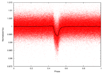
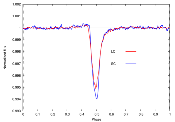
Figure 2: Left: Short cadence Kepler observations (dots) phased with the orbital period. The linear trend was subtracted and data were smoothed (line) with the running window with the width of 0.01. Right: A comparison between the short cadence (SC, blue) and the long cadence (LC, red) Kepler transit light-curves.

3 Evolution of the tail

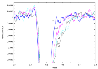
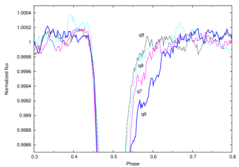
Figure 3: Evolution of the comet-like tail. Left: There is a progressive strengthening of the absorption in the tail between Kepler quarters 3 to 6. Right: There is a progressive diminishing of the absorption in the tail between Kepler quarters 6 to 9.

Apart from the known variability in the transit depth which can easily be seen in the rough data (Rappaport et al. rappaport12 (2012)) there may also be changes in the ’cometary’ tail. These changes are not that easily detected since the tail is much finer and not as deep as the core of the transit. To verify this idea we constructed an averaged light-curve for the long cadence observations during each Kepler quarter with the same method as described in the previous section. In this case, a twice as wide box-car window was used, compared to the previous case. These light-curves were then inspected for variability. One can indeed see in the Figure 3 that there are apparent changes in the tail on the timescale of about 1 yr. Namely, the tail gets more pronounced during quarters 3 to 6, then diminishes during quarters 6 to 9. The story continues and the tail progressively gets stronger during quarters 9 to 11, and again ceases during quarters 11 to 13 but this is not shown in these pictures. This indicates that the changes may be periodic with a period of about one and a half year. Curiously, these changes in the tail on these timescales and in these averaged light-curves can be even stronger than the changes in the transit core which happened during the quarters 3-6! The changes in the tail do not seem to correlate with the changes in the transit core.

The origin of this variability needs to be explored. One can speculate that it may be associated with the magnetic activity of the star or planet. One cannot also exclude that these cycles may originate from the variability in the transit core which reflects the variability of the dense material in the close vicinity of the planet which feeds the tail. In either case and in a more general context this variability represents a new type of star-planet interaction (Shkolnik et al. shkolnik08 (2008)). Note that these changes in the tail might also cause spurious changes in the orbital period due to their asymmetric nature. It indicates that the planet is not uniform and has at least two components: a sort of ’coma’ responsible for the transit core and the tail responsible for the egress.

4 Optical properties of the dust

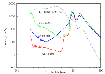
Figure 4: Opacities of forsterite and pyroxene for different iron content. Blue (Frst) - forsterite, red (Fe00) - pyroxene with 0% of iron (enstatite), green (Fe20)- pyroxene with 20% of iron. Solid line - absorption, dashed line - scattering. Calculated assuming the characteristic radius of the grains 1 micron.

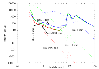
Figure 5: Opacities of pyroxene with 20% of iron as a function of particle radius. Red - 0.01 micron, green - 0.1 micron, blue - 1 micron. Solid line - absorption, dashed line - scattering.

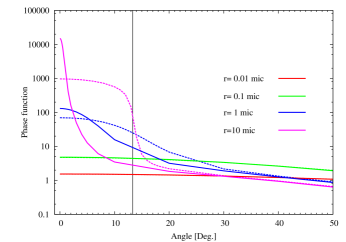
Figure 6: Phase functions at 650 nm for different particle radii. Full line - phase functions assuming a point source of light. Dashed line -phase functions which take into account the finite dimension of the stellar disk. Notice the strong forward scattering peak for larger particles. Vertical line illustrates the angular dimension of the stellar disk as seen from the planet.

According to Rappaport et al. (rappaport12 (2012)) the comet like tail of the planet may consist mainly of dust made of pyroxene grains. Optical properties of the pyroxene and another silicate of the olivine family - forsterite were calculated using Mie theory and Mie scattering code of Kocifaj (kocifaj04 (2004)) and Kocifaj et al. (kocifaj08 (2008)) which is based on Bohren & Huffman (bohren83 (1983)). By optical properties we mean opacities for scattering and absorption and phase functions. The complex index of refraction of pyroxene was taken from Dorschner et al. (dorschner95 (1995)). The complex index of refraction of forsterite was taken from Jäger et al.(jager (2003)). We assumed spherical particles of different sizes. To suppress the ripple structure that would appear in the phase function of spherical mono-disperse particles, the poly-disperse Deirmendjian (deirmendjian64 (1964)) distribution of particle sizes was assumed.

Optical properties of pyroxene ($Mg_{1-x}Fe_{x}SiO_{3}$) in the optical region are quite sensitive to the amount of iron in the mineral. It is illustrated on the example of 1 micron grains in the Figure 4. Opacity in the optical and near infrared for micron size particles is dominated by the scattering. Scattering is not very sensitive to the amount of iron. However, the absorption opacity in the optical and near infrared is very sensitive to the amount of iron and increases with higher iron content. Its direct impact on the spectrum is thus suppressed by the strong scattering. On the other hand, stronger absorption of iron rich pyroxene will lead to enhanced heating of the grains which might affect its sublimation and evaporation. Opacities of forsterite ($Mg_{2}SiO_{4}$) for 1 micron grains are also shown in that picture. Its scattering properties are very similar to pyroxene but it differs in absorption in the optical and near IR regions. Notice, that the total (i.e. absorption plus scattering) opacity is almost gray in the optical and near infrared region for 1 micron grains. The chemical composition of the dust in this system is not known and that is why we carried out calculations for all these species. However, if not mentioned otherwise, (in the light of the above mentioned accounts) we assumed a default model composed of the pyroxene grains with a nonzero iron content ($x=0.2$) where 20% of Mg atoms were replaced by Fe.

This situation may change for particles of different size. Figure 5 compares the opacities of 0.01, 0.1 and 1 micron grains of iron contaminated pyroxene. The true absorption of smaller grains is generally slightly lower in the optical and NIR regions. The scattering opacity overcomes the absorption in the optical and NIR region for larger grains. Notice that scattering on 1 micron grains is rather grey in the optical and NIR region and governs optical properties in the 1-8 micron region. Scattering on intermediate 0.1 micron grains have steep color dependence and governs optical properties at wavelengths shorter than 1 micron. Scattering on even smaller 0.01 micron grains is rather weak and has very strong $\lambda^{-4}$ wavelength dependence characteristic of the Rayleigh scattering regime. Absorption dominates the opacity for such small particles. Absorption also dominates scattering for wavelengths longer than 7 micron for all particle sizes smaller than 1 micron. Consequently, multi-wavelength transit observations in the optical and NIR regions might potentially constrain the particle size in this regime.

The phase functions for three different particle sizes at 6500 Å are illustrated in the Figure 6 as a function of the phase angle. Phase angle is an angle between the original and new scattered beam direction. These phase functions exhibit a strong peak near the phase angle zero which is the so-called forward scattering peak. Larger particles and/or shorter wavelengths tend to have stronger and narrower forward scattering peak than smaller particles and/or longer wavelengths. Importance of this forward scattering for the eclipsing systems during the eclipse was stressed by Budaj (2011a ).

However, these phase functions do not take into account the finite and non-negligible angular dimension of the stellar disk as seen from the planet which is about 26 degrees in the diameter. To take this effect into account one would have to split the stellar disk into elementary surfaces and integrate over the disk. Note that this process is mathematically analogous and similar to the rotational broadening of the stellar spectra. The difference is that while in the calculations of the rotational broadening the star is split into strips with constant radial velocity, in the calculation of the scattered light, the star may be split into arcs with constant phase angle. For phase angles greater than $R^{*}/a$, where $R^{*}$ is the star radius and $a$ is the semi-major axis, this approximation will be much more realistic than the point source approximation since the arcs will resemble the strips. This regime involves also the pre-transit brightening (see Section 5). For smaller angles it will not be that good. Consequently, we convolve the phase functions with the ’rotational’ broadening function (BF, Rucinski rucinski02 (2002)) of the star expressed in the angular units. This function is an ellipse with the width corresponding to the angular dimension of the star as seen from the planet and takes into account the linear limb darkening of the stellar surface. We used the limb darkening coefficients from Claret (claret00 (2000)) (see the next section).

One has to be cautious and calculate the phase functions with a very fine step near the zero angle because of the strong forward scattering and, consequently, its convolution with the BF with a very fine step near the edge of the broadening ellipse. These phase functions which take into account the finite dimension of the source of light are also depicted in the Figure 6 for comparison. One can see that the finite dimension of the source of light is important for larger particles but has almost no effect for particles smaller than 0.1 micron. Broadened phase functions are re-normalized to 4$\pi$ during the calculations.

5 Light-curve modelling

In this section we calculate light-curves of the exoplanet using the code SHELLSPEC. This codes calculates the light-curves and spectra of interacting binaries or exoplanets immersed in the 3D moving circum-stellar (planetary) environment. It solves simple radiative transfer along the line of sight and the scattered light is taken into account under the assumption that the medium is optically thin. It is written in Fortran77 but there is also a recent Fortran90 version (Šejnová et al. sejnova12 (2012)). The code was modified so that it is possible to model dusty objects with comet like tails. For this purpose a few new objects (structures) were introduced into the code and studied. They have the form of a cone, ring or an arc with a variable cross-section. Phase functions and dust opacities can be pre-calculated, loaded in the form of a table and interpolated to a particular wavelength during the execution of the program.

In these calculations the star is assumed to be a sphere with the radius of $R^{*}=0.65R_{\odot}$, mass of 0.7 $M_{\odot}$ and be subject to the limb darkening. We used quadratic limb darkening coefficients for R filter from Claret (claret00 (2000)) which are based on the Kurucz models. They were interpolated from the grid assuming an effective temperature of $T_{\rm eff}=4300$K, surface gravity of $\log g=4.63$ (cgs), metallicity of $[M/H]=0.$, and micro-turbulent velocity of $v_{t}=2$ km s^-1. Given the fact that the transit is sometimes missing in the observations, the planet itself must be rather small. It is its comet like tail which gives rise to the major drop in the light-curve. Consequently, the planet is modelled as a 3D object in the form of a ring (or part of the ring) with the radius of $a=2.8R_{\odot}$ and a non negligible thickness (geometrical cross-section). This cross-section, $C$, of the ring and dust density, $\rho$, along the ring are allowed to change with the angle, $t$ in [rad], in the following way:

$$\rho(t)=\rho(0)\frac{C(0)}{C}[|t-t(0)|/\pi+1]^{A1}\leavevmode\nobreak\ \leavevmode\nobreak\ \leavevmode\nobreak\ \leavevmode\nobreak\ or$$ (2)

$$\rho(t)=\rho(0)\frac{C(0)}{C}e^{|t-t(0)|/\pi*A2}.$$ (3)

Where $\rho(0),C(0),t(0)$ is the dust density, cross-section and angle at the beginning of the arc, and $A1,A2$ are the density exponents to model additional phenomena e.g. dust destruction. The ring was located in the orbital plane. In the following we describe the effect of various free parameters on the light-curve of this object.

Inclination. We carried out a sequence of calculations for the most straightforward assumption that the ring is in the orbital plane of the planet and that this orbital plane has an inclination of $i=90$ deg with respect to the plane of sky. It turned out that the observed core of the transit is too sharp. This indicates that the transit is not entirely edge on but may have $i<84$ deg. An alternative, explanation, could be that the $R^{*}/a$ parameter is overestimated or that the dust particle size in the close vicinity of the planet is larger, which could narrow the transit by filling its ingress and egress by the scattered light with sharper forward scattering peak. There is an interesting effect that smaller inclinations or grazing transits require slightly higher dust densities and that the forward scattering peak gets more pronounced. Ultimately, for the non-transiting planet, the light-curve shows the transit brightening only. The inclination $i=82$ seems to reproduce the observations well and, if not mentioned otherwise, we will use this as a default value in the following calculations. This value corresponds to the impact parameter $b=0.60$ expressed relative to the stellar radius or $b=0.39R_{\odot}$ in absolute units. It is in agreement with the result of Brogi et al. (brogi12 (2012)) who estimated several values of the impact parameter in the range 0.46-0.63.

Geometrical cross-section of the tail. Unfortunately, this quantity cannot be constrained very well. There is a strong degeneracy between this quantity, dust density and optical depth along the line of sight. It stems from the Eqs. 2 3 and best fitting light-curves tend to have the same product $\rho C$. An increase in the cross-section by a factor of 2 results in decreasing the dust density by a factor of 2 and decreasing the optical depth through the tail by the same factor.

Dust density profile. The shape of the transit is highly asymmetric with steep ingress and long shallow egress. This is the main argument for the idea of a comet-like tail and it suggests that the dust density decreases steeply along the tail. This density profile is described by the Eqs. 2 and 3 and is one of the most important free parameters. This is illustrated in the Figure 7 which was calculated assuming $i=82$ deg, characteristic particle size of about 0.1 micron, and iron contaminated pyroxene. The best results are achieved when $A1,A2$ are about -20 and it will be our default value when studying other effects. This is a very steep function of angular distance from the planet and it indicates that the dust grains are either effectively destroyed or removed from the tail. Higher exponents fit the core better while lower exponents fit the tail better. This also suggests that the object may consists of two different components. Each density exponent requires different density $\rho(0)$ to fit the depth of the transit properly and this depends also on the particle size and the chemical composition of the dust. In the Table 1 we give the dust density $\rho(0)$ and the maximum optical depth through the tail in front of the star corresponding to a particular density exponent for three kinds of species: pyroxene with 20% of iron, enstatite (pyroxene with 0% of Fe), and forsterite. The calculations assumed an inclination of 82 degrees and the geometrical cross-section at the beginning and end of the tail of 0.01 and 0.09 $R_{\odot}^{2}$, respectively. Notice that the density of the Fe contaminated pyroxene and enstatite do not differ considerably for larger particles but enstatite requires higher densities for smaller particles. This is because opacity at these wavelengths for larger particles is dominated by the scattering which is not affected by the Fe content while opacity of smaller grains is dominated by the absorption and pyroxenes with higher Fe content have higher optical opacity. Densities of forsterite do not differ much from those of enstatite and are only slightly lower for smaller particles.

Figure 8 illustrates the difference between the power law behaviour (Eq.2) and the exponential behaviour (Eq.3) for $A1=A2=-20$, $\rho(0)=5\,10^{-15}$, for an iron contaminated pyroxene with 1 micron grains. There is only a little difference and an exponential profile fits the core slightly better while a polynomial profile fits the tail slightly better.

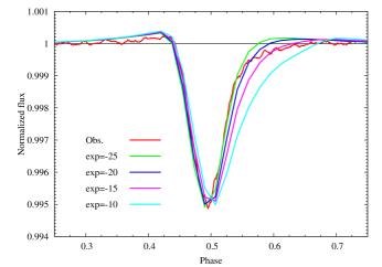
Figure 7: The effect of the dust density profile on the light-curve. Higher exponents fit better the core while lower exponents fit better the tail. In any case, the dust density in the tail rapidly decreases with the (angular) distance from the planet which indicates that the dust is either quickly destroyed or scattered out of the tail.

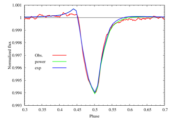
Figure 8: The comparison between the exponential (exp) and power law (power) density profile. Both profiles are very similar, exponential profile fits slightly better the core while a polynomial profile fits slightly better the tail (see the text).

Table 1: Density exponent $A2$, dust density $\rho(0)$ at the edge of ring $\times 10^{-15}$ g cm^-3, and maximum optical depth $\tau$ for pyroxene with 20% of iron, enstatite, forsterite and for various dust particle radii. Model assumes that the geometrical cross-section of the ring is 0.01 and 0.09 $R_{\odot}^{2}$ at the beginning and the end of the ring, respectively.

	pyroxene		enstatite		forsterite
A2	$\rho$	$\tau$	$\rho$	$\tau$	$\rho$	$\tau$
0.01 micron
-10	42	0.066	110	0.064	90	0.064
-15	54	0.081	150	0.082	120	0.080
-20	66	0.095	178	0.094	145	0.094
-25	79	0.110	215	0.11	177	0.11
0.1 micron
-10	0.26	0.075	0.30	0.073	0.26	0.072
-15	0.33	0.091	0.38	0.086	0.33	0.086
-20	0.41	0.110	0.46	0.10	0.40	0.10
-25	0.49	0.120	0.56	0.12	0.49	0.12
1 micron
-10	3.0	0.14	3.0	0.13	3.0	0.13
-15	3.8	0.17	3.8	0.15	3.8	0.15
-20	4.6	0.19	4.6	0.18	4.6	0.18
-25	5.6	0.23	5.6	0.21	5.6	0.21

Particle size. This parameter is very important since it affects the absorption and scattering opacity and emissivity which is illustrated in the Figure 5. Unfortunately, due to this dependence there is a strong degeneracy between this parameter, dust density and geometrical cross-section of the tail. This degeneracy is demonstrated in the Figure 9 which depicts a comparison between the theoretical light-curves and Kepler short cadence observations. It is possible to fit the transit with dust particles of different size and different dust densities. This degeneracy complicates precise estimates of the particle size and dust density from the shape of the transit. In the Table 1 we list various possible combinations of the edge density and density exponent for different particle radii and different grains. Notice that 0.1 micron particles require substantially lower dust densities to reproduce the transit than 1 micron particles which in turn require much lower densities than 0.01 micron particles. This can be understood using the Figure 5 which shows that at 600 nm the opacity is dominated by the scattering on 0.1 micron particles followed by the scattering on 1 micron particles, and absorption on 0.01 micron grains.

Nevertheless, particle size does leave a few interesting imprints on the light-curve. Notice the strong pre-transit brightening and a less pronounced post-transit brightening which are quite sensitive to the particle size. It is best seen in the long cadence observations since there are more of them and have less scatter compared to the short cadence data (see Figure 10). The pre-transit brightening is caused by the strong forward scattering. This forward scattering is strongly sensitive to the particle size as demonstrated in the Figure 6. This is why the pre-transit brightening is so sensitive to the particle size and can be used to estimate the dust particles size. Larger size particles (0.1-1 micron) or they combination fit better the transit core and the pre-transit brightening while smaller size particles (0.01-0.1 micron) or their combination fit better the slow egress and post-transit brightening. This is just another indication that the planet is not uniform. The particle size may decrease as a function of the angular distance from the planet which can be considered as an indication for the dust destruction in the tail. Notice that the larger particles exhibit a narrower transit than the smaller particles. This is because larger particles fill the ingress and egress by the strong forward scattered light. This may cause another degeneracy between the particle size, orbital inclination, and density exponent since they all affect the width of the transit. In an independent analysis, Brogi et al. (brogi12 (2012)) using different model and analysis estimated the particle size of about 0.1 micron in the tail. However, in their analysis they did not use real dust opacities, phase functions were approximated by the analytical Henyey-Geenstein phase functions, and the finite radius of the source of light was ignored.

The latest Kepler short cadence observations are also very helpful in constraining the particle size. Their comparison with the theoretical light-curves is in Figure 11. If the calculations are to be interpreted solely in terms of the particle size then the phases 0.3-0.4 are best reproduced by 1 micron particles. Phases at about 0.45 might be affected and screened by the streams mentioned in the next section which are not modelled here. Phases 0.5-0.55 are best reproduced by the 1 micron particles. Phases near 0.55-0.57 are best fit with the 0.1 micron particles whereas even later phases further in the tail are best reproduced with particles that have radii of about 0.01 micron. Alternative explanation could be that the tail is composed of several chemical or structural components which have different A1 or A2 parameters or destruction lifetimes.

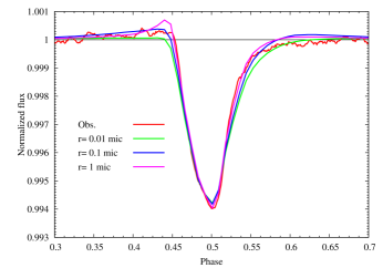
Figure 9: Short cadence observations vs the models. The effect of the particle size on the light-curve. There is a strong degeneracy between this parameter and dust density. However, notice that larger size particles fit better the transit core whereas smaller size particles fit better an extended egress.

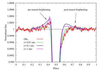
Figure 10: A more detail look on the effect of the particle size on the light-curve. Long cadence observations vs models. Notice a significant pre-transit brightening and less significant post-transit brightening which are caused by the strong forward scattering. It is rather sensitive to the particle size. Dust particles with typical radii of about 0.1-1 micron fit better the transit core whereas 0.01-0.1 micron particles fit better an extended egress and post transit brightening.

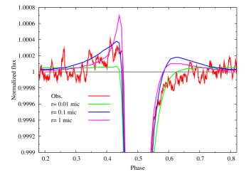
Figure 11: The same as in Figure 10 but for the Kepler short cadence observations. The phases 0.3-0.4 are best reproduced by 1 micron particles, phases at about 0.45 might be affected and screened by the streams which are not modelled here, phases 0.5-0.55 are best reproduced by the 1 micron particles, phases near 0.55-0.57 are best fit with the 0.1 micron particles whereas later phases further in the tail are best reproduced with particles that have radii of about 0.01 micron.

Tail morphology. The above mentioned ring/arc morphology of the tail seems to reproduce the observations surprisingly well. The tail is about 60 degrees long. The density in the tail decreases rapidly along the tail and becomes negligible beyond 60 degrees from the planet. Apart from the clear pre-transit brightening, notice a weak post-transit brightening in the Figure 10. This can happen if the tail is terminated by a relatively sudden drop in the density or is dispersed out of the orbital plane, reaches the vertical thickness greater than the radius of the star and there is still a small but non negligible fraction of particles with the size of the order 0.1 micron. Apart from the above mentioned tail morphology, I tried also some other geometrical models. For example, a dusty tail of the shape of a cone pointing at different angles from the planet. Such geometry would produce very strong post-transit brightening which would not be compatible with the observations.

Theoretical light-curve for 1 micron particles fits the pre-transit brightening best but shows a slight excess compared to the observations. This is best seen in the comparison with the short cadence observations in the Figure 11. This excess might disappear if a more realistic model of the dust morphology is considered. Notice, that hydrodynamical simulations of Bisikalo et al. (bisikalo13 (2013)) predict two streams emanating from the planet. One leaves the planet via the L2 point and is deflected in the direction opposite to the orbital movement which might result into the comet like tail like the one we observe and model here. The other leaves the planet via the L1 point and is deflected in the direction of the orbital motion. This stream is well known in the interacting binaries. Such stream might wipe out the excess emission in the pre-transit brightening seen in the theoretical light-curves. We do not model this second stream in this paper since we consider it too premature at this point.

Our model of the planet and what happens during the transit is illustrated in the Figure 12. This is a 2D image of the model which shows the logarithm of the intensity. One can clearly see the tail with a very steep intensity gradient which becomes much brighter close to the star due to the forward scattering and density gradient. Notice also the optically thin absorption on the stellar disk.

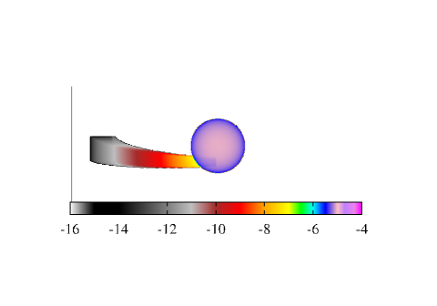
Figure 12: A 2D image (logarithm of intensity) of the planet with a comet-like tail during the transit. One can clearly see the tail. Its intensity rapidly decreases due to decreasing dust density and strong forward scattering. Notice also the optically thin absorption on the limb darkened stellar disk. Calculated for 1 micron pyroxene grains.

KIC 12557548b in the more general context. It is very interesting to note that this pre-transit brightening is analogous to the mid-eclipse brightening (MEB) observed in some long period eclipsing binaries like $\epsilon$ Aur (Budaj 2011a ) or AZ Cas (Galan et al. galan12 (2012)). MEB in $\epsilon$ Aur may be due to dark flared dusty disk eclipsing F super-giant and forward scattering plays an important role. MEB in AZ Cas may also be caused by the forward scattering during the primary eclipse. During this eclipse the hotter B star is eclipsed by the cool M super-giant. Dust surrounding the cool component can scatter the light from the hidden hot star to the observer. Such effect was predicted and calculated in Section 2 of Budaj 2011a . Since very similar dust properties and physics can explains the light-curves of all three objects it gives stronger footing to our explanation of the shallow MEB in $\epsilon$ Aur. This model is in contrast with the geometrical model of the inclined disk and the star peeking through the hole. In spite of the fact that these are very different objects it looks like they are subject to similar physical processes, can be modelled with similar tools, and the knowledge obtained in one, can be applied to the other. This analogy suggests that there might also be a tail of dust emanating from the disk of $\epsilon$ Aur which could explain non-symmetric behaviour of gas and dust absorption during the eclipse with egress absorption being stronger and longer (Martin et al. martin13 (2013), Leadbeater et al. leadbeater13 (2013)). On the other hand there might be a dusty disk formed inside the Hill sphere of KIC12557548b which would feed into the comet-like tail.

There is one more thing which needs to be mentioned. Long cadence observations have a relatively long exposure (30 min) which might smear any potential sharp features in the light curve. That is why the theoretical light-curves were convolved with the box-car which had a width corresponding to the exposure time (0.031 phase units). Short cadence observations have exposure time (1min) which is much shorter than the box-car smoothing applied to the observed data. Consequently, theoretical light-curves used for comparison with the short cadence data were smoothed with the box-car which had a width corresponding to the box-car width applied to the observations (0.01 in phase units). This had very little effect on the result.

6 Conclusions

The light-curve of this planet candidate was reanalysed using first 14 quarters of the Kepler data including first short cadence observations.

Orbital period of the planet was improved. We searched for the long term period changes but found no convincing evidence of such changes.

Quasi periodic variability in the tail of the planet with the period of about 1.5 year was discovered.

We modelled the light-curve of KIC012557548 using SHELLSPEC code with the following assumptions: spherical dust grains, different dust species (pyroxene, enstatite, forsterite), different particle sizes, Mie absorption and scattering, finite radius of the source of light (star) and that the medium is optically thin. We proved that its peculiar light-curve is in agreement with the idea of a planet with a comet like tail. A model with a dusty ring in the orbital plane which has an inclination of about 82 degrees, exponential or power law density profile ($A1=A2=-20$) fits the observations surprisingly well.

We confirmed that the light-curve has a prominent pre-transit brightening. There is an indication of a less prominent brightening after the transit, both are caused by the forward scattering.

Dust density in the tail is a steep decreasing function of the distance from the planet which indicates significant destruction of the tail caused by the star.

Transit depth is a highly degenerate function of the particle size, dust density, and other dust properties. Various combinations of them were estimated and tabulated. There will also be a degeneracy between the inclination, particle size, and the density exponent.

However, the forward scattering and the pre(post)-transit brightening are quite sensitive to the particle size. Consequently, we estimated the particle size (radius) of the grains in the head of the tail from the pre-transit brightening to be about 0.1-1 micron. There is an indication that the particle size is larger at the head and decreases along the tail to about 0.01-0.1 micron.

We argue that there are several indications that the ’planet’ is not homogeneous and that it consists of several components. The component that is responsible for the transit core and the other responsible for the tail. Components may have different grains with different density profiles, and/or particle size.

It is interesting to note that this planet’s light-curve with pre-transit brightening is analogous to light-curves of some interacting binaries with mid-eclipse brightening, particularly $\epsilon$ Aur and forward scattering plays an important role in all of them.

- (1) Bisikalo, D., Kaygorodov, P., Ionov, D., Shematovich, V., Lammer, H., & Fossati, L. 2013, ApJ, 764, 19
- (2) Bohren C. F., & Huffman D. 1983, Absorption and scattering of light by small particles. Wiley, New York, 530 pp
- (3) Borucki, W.J. et al. 2011, ApJ, 736, 19
- (4) Brogi, M., Keller, C.U., Ovelar, M. de Juan, Kenworthy, M.A., de Kok, R.J., Min, M. & Snellen, I.A.G. 2012, A&A, 545, L5
- (5) Budaj, J. 2011a, A&A, 532, L12
- (6) Budaj, J., & Richards, M.T. 2004, Contrib. Astron. Obs. Skalnaté Pleso, 34, 167
- (7) Carroll, S.M., Guinan, E.F., McCook, G.P., & Donahue, R.A. 1991, ApJ, 367, 278
- (8) Claret, A. 2000, A&A, 363, 1081
- (9) Deirmendjian, D. 1964, Appl. Opt., 3, 187
- (10) Dorschner, J., Begemann, B., Henning, T., Jaeger, C., Mutschke, H. 1995, A&A, 300, 503
- (11) Faigler, S. & Mazeh, T. 2011, MNRAS, 415, 3921
- (12) Galan, C., Tomov, T., Mikolajewski, M., Swierczynski, E., Wychudzki, P., Bondar, A., Kolev, D., Brozek, T., Drozd, K., & Ilkiewicz, K. 2012, IBVS, 6027, 1
- (13) Guinan, E.F. et al. 2012, A&A 546, A123
- (14) Hoard, D. W., Howell, S. B., & Stencel, R. E. 2010, ApJ, 714, 549
- (15) Jackson, B.K., Lewis, N.K., Barnes, J.W., Drake D.L., Showman, A.P., & Fortney, J.J. 2012, ApJ, 751, 112
- (16) Jäger, C., Dorschner, J., Mutschke, H., Posch, T., & Henning,T. 2003, A&A, 408, 193
- (17) Kocifaj, M. 2004, Contrib. Astron. Obs. Skalnate Pleso 34, 141 156
- (18) Kocifaj, M., Klacka, J., & Posch, T. 2008, Astrophys. Space Sci. 317, 31
- (19) Leadbeater, R., Buil, C., Garrel, T., Gorodenski, S.A., Hansen, T., Schanne, L., Stencel, R.E., & Stober, B. 2013, The Journal of the American Association of Variable Star Observers, 40, 729
- (20) Lecavelier Des Etangs, A., Vidal-Madjar, A., & Ferlet, R. 1999, A&A, 343, 916
- (21) Mandel, K., &y Agol, E. 2002, ApJ, 580, L171
- (22) Martin, J.C., Foster, C., & O’Brien, J.A. 2013, AAS Meeting, #221, #252.18
- (23) Mura, A., et al. 2011, Icarus, 211, 1
- (24) Muthumariappan, C., & Parthasarathy, M. 2012, MNRAS, 423, 2075
- (25) Perez-Becker, D., Chiang, E. 2013, eprint arXiv:1302.2147
- (26) Rappaport, S., Levine, A., Chiang, E., El Mellah, I., Jenkins, J., Kalomeni, B., Kite, E. S., Kotson, M., Nelson, L., Rousseau-Nepton, L., & Tran, K. 2012, ApJ, 752, 1
- (27) Rucinski, S. 2002, AJ, 124, 1746
- (28) Schneider, J., Rauer, H., Lasota, J.P., Bonazzola, S., & Chassefiere, E. 1998, in: Brown dwarfs and extrasolar planets, ASP Conference Series 134, eds. Rafael R., Eduardo L.M., Maria Rosa Zapatero O., p. 241.
- (29) Shkolnik, E., Bohlender, D.A., Walker, G.A.H., Collier Cameron, A. 2008, ApJ, 676, 628
- (30) Šejnová, K., Votruba, V., & Koubský, P. 2012, in: From Interacting Binaries to Exoplanets: Essential Modeling Tools, eds. M. T. Richards, I. Hubeny, IAU Symposium, Volume 282, p. 261
- (31) Southworth, J. 2012, MNRAS, 426, 1291
- (32) Stellingwerf, R. F. 1978, ApJ, 224, 953