The Opacity of the Intergalactic Medium during Reionization: Resolving Small-Scale Structure

Abstract

Early in the reionization process, the intergalactic medium (IGM) would have been quite inhomogeneous on small scales, due to the low Jeans mass in the neutral IGM and the hierarchical growth of structure in a cold dark matter Universe. This small-scale structure acted as an important sink during the epoch of reionization, impeding the progress of the ionization fronts that swept out from the first sources of ionizing radiation. Here we present results of high-resolution cosmological hydrodynamics simulations that resolve the cosmological Jeans mass of the neutral IGM in representative volumes several Mpc across. The adiabatic hydrodynamics we follow are appropriate in an unheated IGM, before the gas has had a chance to respond to the photoionization heating. Our focus is determination of the resolution required in cosmological simulations in order to sufficiently sample and resolve small-scale structure regulating the opacity of an unheated IGM. We find that a dark matter particle mass of $m_{\rm dm}\lesssim 50~{}M_{\odot}$ and box size of $L\gtrsim 1$ Mpc are required. With our converged results we show how the mean free path of ionizing radiation and clumping factor of ionized hydrogen depends upon the ultraviolet background (UVB) flux and redshift. We find, for example at $z=10$, clumping factors typically of 10 to 20 for an ionization rate of $\Gamma\sim 0.3-3\times 10^{-12}$s^-1, with corresponding mean free paths of $\sim 3-15$ Mpc, extending previous work on the evolving mean free path to considerably smaller scales and earlier times.

1. Introduction

The fact that the most abundant sources of radiation during reionization are likely to be currently undetectable (e.g., Trenti et al., 2010; Oesch et al., 2012; Alvarez et al., 2012) means that the details of the reionization process are beyond most current observational probes. The notable exceptions are observations of the polarization of the cosmic microwave background (CMB), which imply an optical depth to Thomson scattering of $\tau\sim 0.09$ (Komatsu et al., 2011), and the appearance of a Gunn-Peterson trough in the spectra of distant quasars (Fan et al., 2006), indicating that reionization was largely complete by $z\sim 6$. Reionization is therefore thought to have mainly taken place over the redshift range $z\sim 6-15$. Due to the lack of more specific constraints, much of our current understanding about the epoch of reionization comes from theoretical studies in the context of the $\Lambda$CDM cosmology.

The picture which always emerges is of small-scale gaseous structures forming at $z>20$, due to the collapse of dark matter halos at the Jeans scale, roughly $10^{4}~{}M_{\odot}$ (e.g., Peebles & Dicke, 1968; Couchman & Rees, 1986; Shapiro et al., 1994; Gnedin & Hui, 1998). The gas was just cool enough to fall into halos at this mass, leading to strong inhomogenities on a scale of tens of comoving parsecs. At the same time, slightly more massive halos, with masses on the order of $\sim 10^{6}~{}M_{\odot}$, formed enough H₂ molecules in their cores to cool efficiently, leading to the formation of the first stars in the Universe (e.g., Tegmark et al., 1997; Abel et al., 2002; Bromm et al., 2002; Yoshida et al., 2003). The ionizing radiation from these stars is thought to have created substantial, yet short-lived H II regions, which were shaped by the surrounding inhomogeneity of the gas distribution (Alvarez et al., 2006; Abel et al., 2007; Yoshida et al., 2007).

Eventually, sufficiently large halos formed that triggered the formation of the first galaxies (Johnson et al., 2007; Wise & Abel, 2008; Greif et al., 2008). These nascent dwarf galaxies would have created longer-lived and isolated H II regions (Wise & Cen, 2009; Wise et al., 2012). It is unclear how these galaxies evolved into the much more luminous ones that have been observed at redshifts as high as $z\sim 8$ (e.g., Bouwens et al., 2010). Nevertheless, it is widely believed that as the first galaxies grew and merged, their collective radiative output created a large and complex patchwork of ionized bubbles, with characteristic sizes on the order of tens to hundreds of comoving Mpc (e.g., Barkana & Loeb, 2004; Furlanetto et al., 2004; Iliev et al., 2006). During this time, dense systems in the IGM likely impeded the progress of ionization fronts (Barkana & Loeb, 1999; Haiman et al., 2001; Shapiro et al., 2004; Iliev et al., 2005a; Ciardi et al., 2006). At the end of reionization the so-called “Lyman-limit” systems, dense clouds of gas optically-thick to ionizing radiation observed in the spectra of quasars at $z<6$ (e.g., Storrie-Lombardi et al., 1994; Prochaska et al., 2009), dominated the overall opacity of the IGM to ionizing radiation. These systems crucially influenced the percolation phase of reionization (Gnedin & Fan, 2006; Choudhury et al., 2009; Alvarez & Abel, 2012), which in turn determined the evolution and structure of the ionizing background (e.g., Haardt & Madau, 1996; Bolton & Haehnelt, 2007; McQuinn et al., 2011).

Thus, the progress of reionization depended not only on the properties of the sources of ionizing radiation, but also on the sinks. Theoretical models of reionization must describe not just the spectral energy distribution, abundance, and clustering of early sources of ionizing radiation, but also the inhomogeneity of the intergalactic medium (IGM) in the space between the sources. It is this latter description that is the goal of the present work.

Early descriptions of reionization took into account inhomogeneities in the IGM through a “clumping factor”, $c_{l}$, by which the recombination rate is boosted relative to the homogeneous case. This allows one to write a global ionization rate, equal to the ionizing photon emmissivity minus the recombination rate of a clumpy IGM, and thereby determine the reionization history for a given ionizing source population. Shapiro & Giroux (1987) used such a model to show that the observed population of QSOs were insufficient to have reionized the Universe by $z\sim 5$. Their assumption of $c_{l}\sim 1$ would have been conservative, in that that additional recombinations would have made it even more difficult for quasars alone to reionize the Universe.

In addition to being useful in modeling the reionization history, the clumping factor is also important in estimating the necessary number of ionizing photons per baryon to maintain an ionized Universe. The necessary and sufficient condition for maintaining an ionized Universe is that the ionizing photon emissivity should be greater than or equal to the recombination rate of the IGM. Madau et al. (1999) used this fact to derive a critical star formation rate, above which the rate of ionizing photons is enough to maintain the Universe in an ionized state.

Gnedin & Ostriker (1997) used hydrodynamic simulations with a treatment of photoionization in the “local optical depth” approximation to determine the clumping factor of the ionized component of the IGM, finding a value of $c_{l}\sim 30$ at $z=6$. They also pointed out that the actual clumping factor of the IGM would have been larger due to structure on smaller scales than they resolved. More recently, Miralda-Escudé et al. (2000) built a semi-analytical model for the reionization of an inhomogenous IGM, in which the underlying gas density distribution was determined by numerical simulations. They argued that in addition to specifying the clumping factor of the ionized medium, it is also necessary to describe the distribution of high-density gas clouds that are able to self-shield against ionizing radiation.

McQuinn et al. (2011) followed a similar approach to that of Miralda-Escudé et al. (2000) to explain the evolution of the ionizing background radiation at redshifts less than $z\sim 6$, using more realistic numerical simulations which were post-processed with radiative transfer. These works were focused on the large scales relevant in the post-reionization IGM, after photoionization heating has “ironed out” the clumpiness of the IGM on the smallest scales. The timescale over which this smoothing occurs is on the order of $10-100$ Myr (Iliev et al., 2005b). Although the recombination rate in the homogenous IGM is on the order of 1 Gyr, small-scale inhomogeneities increase recombinations by at least an order of magnitude, making the recombination time of the high-redshift IGM comparable to the smoothing time. Our work here is focused on the higher redshifts and smaller scales that were most relevant early in reionization before much smoothing has occurred.

We seek to obtain convergence in the quantities that describe the inhomogeneity of the unheated IGM during the epoch of reionization, such as the mean free path, $\lambda$, clumping factor, $c_{l}$, and density threshold above which gas is self-shielded, $\Delta_{\rm crit}$, by spanning the parametre space of redshift and ionizing background intensity, $j_{\nu}$. To do this, we post-process cosmological adiabatic hydrodynamics simulations with radiative transfer calculations along different lines of sight through the simulated volume. Radiative feedback raises the Jeans mass of the IGM, thereby increasing the scale of inhomogeneities. Therefore, the resolutions we find in our adiabatic simulations that are necessary to resolve structure in the unheated IGM are also sufficient to model radiative feedback at all times.

The outline of the paper is as follows. Details of the simulation setup and radiative transfer are described in $\S 2$. In $\S 3$ we present our numerical results, followed by $\S 4$, where we present the results of our convergence tests. $\S 5$ concludes with a discussion of our main results.

Table 1Simulation Parameters

Simulation	$N$	$L$ (Mpc)	$m_{\rm dm}$ ($M_{\odot}$)	$r_{\rm soft}$ (pc)
A1	$2\times 256^{3}$	0.25	31	30
A3	$2\times 256^{3}$	1	$2.0\times 10^{3}$	120
A4	$2\times 256^{3}$	2	$1.6\times 10^{4}$	240
A6	$2\times 256^{3}$	8	$1.0\times 10^{6}$	960
B1	$2\times 512^{3}$	0.25	3.8	15
B2	$2\times 512^{3}$	0.5	31	30
B3	$2\times 512^{3}$	1	240	60
B4	$2\times 512^{3}$	2	$2.0\times 10^{3}$	120
B5	$2\times 512^{3}$	4	$1.6\times 10^{4}$	240
B6	$2\times 512^{3}$	8	$1.3\times 10^{5}$	480
C1	$2\times 1024^{3}$	0.25	0.5	7.5
C2	$2\times 1024^{3}$	0.5	3.8	15
C3	$2\times 1024^{3}$	1	31	30
C4	$2\times 1024^{3}$	2	240	60
C6	$2\times 1024^{3}$	8	$1.6\times 10^{4}$	240

2. Numerical Approach

Here we describe our numerical approach, in which we perform a suite of cosmological adiabatic hydrodynamics simulations using the publicly available SPH code Gadget-2 (Springel, 2005). We then postprocess each simulation with multifrequency radiative transfer of hydrogen ionizing radiation, assuming photoionization equilibrium, to determine the dependence of basic quantities, like the ionizing photon mean free path and clumping factor, on redshift and intensity of the background radiation field. The mean free path presented here is used to quantify the opacity of the IGM to ionizing radiation and should be considered a local quantity that depends on the spatial variation of the UVB flux during patchy reionization.

2.1. Cosmological Hydrodynamic Simulations

The cosmological simulations are parameterized by box size, $L$, and total number of dark matter and gas particles, $N$. Table LABEL:table:simparams summarizes these parameters for our suite of simulations and lists their corresponding dark matter particle masses, $m_{\rm dm}$, along with the comoving gravitational softening length, $r_{\rm soft}$. The simulations were evolved from redshift $z=200$ to $z=6$, except for simulations C1 through C4 which, due to computational limitations, were terminated early at $z=10$. Initial conditions were generated separately for dark matter and baryons using transfer functions computed by CAMB for each component, with the same random phases. Throughout our work we assume the set of cosmological parameters ($\Omega_{\mathrm{DM}}$, $\Omega_{\mathrm{b}}$, $\Omega_{\Lambda}$, $h$) = (0.228, 0.042, 0.73, 0.72).

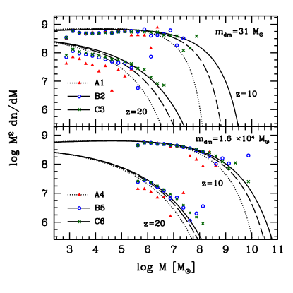
Figure 1.— Halo mass functions from six simulations are compared to their Warren et al. counterparts using the variance $\sigma_{\rm eff}^{2}\equiv\sigma^{2}-\sigma^{2}(M_{\rm box})$ at redshifts 10 and 20. The top panel plots simulations A1, B2, and C3 each containing dark matter masses of $m_{\rm dm}=31~{}M_{\odot}$ while the lower panel plots simulations A4, B5, and C6 with $m_{\rm dm}=1.6\times 10^{4}~{}M_{\odot}$. In each case, points denote halo mass functions obtained from the simulations while the lines trace the corresponding Warren et al. curves.

A quantitative test of the simulated structure formation is to identify dark matter halos to construct mass functions, $dn/dM$, which can be compared to analytic models. Figure 1 shows the mass functions obtained from a friends-of-friends (FOF) halo identification scheme with linking length of 0.2 mean interparticle spacings, at redshifts $z=10$ and 20 for two groups of simulations sharing common mass resolutions of $m_{\rm dm}=31~{}M_{\odot}$ and $1.6\times 10^{4}~{}M_{\odot}$. A common fitting function to compare to is the Warren et al. (2006) mass function. When doing so, however, it is important to note that this model assumes a Universe with infinite spatial extent; something that cannot be achieved using numerical simulations. It is therefore useful to compute Warren et al. mass functions using a modified variance of the form $\sigma_{\rm eff}^{2}\equiv\sigma^{2}-\sigma^{2}(M_{\rm box})$, where $M_{\rm box}$ is the total mass contained within the simulated volume. This has the effect of removing contributions from mass fluctuations on scales larger than that of the simulated volume. With this correction we find that the Warren et al. mass function is generally well-matched by the numerical simulations.

There is one important feature worth noting in Figure 1: For fixed mass resolution, simulations with larger volumes tend to trace the analytic curves more closely. This is most noticeable in the top panel for $z=20$. We can attribute this to the fact that at fixed resolution, simulations with larger volumes will contain a more statistically representative collection of halos. In $\S$4 we will show how sample variance in small boxes has important consequences for numerical convergence. Even though a simulation may have a sufficient mass resolution to resolve low-mass halos within the IGM, its volume may be so small that sample variance causes noticeable variation in computed quantities between different random realizations. Recall that we used a modified variance $\sigma_{\rm eff}^{2}$ when computing the analytic curves of Figure 1 in order to compensate for missing large-scale power in the finite volume boxes. Though not necessary for our purposes here, we point out to the reader that Reed et al. (2007) present an additional correction that can be used to adjust simulated mass functions for sample variance from small volumes.

It is well known that the inhomogeneous nature of the IGM plays an important role in the progression of the reionization epoch. This was emphasized by Miralda-Escudé et al. (2000) who presented an evolutionary model of reionization based on the gas density distribution observed in numerical simulations. It is therefore useful to examine the density distribution of baryons within cosmological simulations, through the use of the probability density function (PDF), $P(\Delta)$, defined to be the normalized distribution of gas in terms of overdensity $\Delta\equiv\rho/{\overline{\rho}}$.

In Figure 2 we plot volume-weighted gas PDFs from our fiducial simulation B2 which contains $2\times 512^{3}$ dark matter plus gas particles in a box of comoving length 0.5 Mpc. More precisely, we plot $\Delta^{2.5}P(\Delta)$ which is expected to approach a constant at $\Delta>\Delta_{\rm vir}=18\pi^{2}$ if gas at those densities is collapsed within halos described by a density profile $\rho\propto r^{-2}$. As time evolves, the fraction of gas collapsed within halos increases, though only for $z\lesssim 10$ does the high-density tail of the PDF appear to approach a constant value.

Recall that the PDFs shown here correspond to adiabatic simulations for which radiative heating and cooling processes are ignored. We expect that heating would evolve the gas distribution in such a way as to decrease the amplitude of $P(\Delta)$ at large values of $\Delta$ as gas boils out of overdense regions. In this work we are concerned with the initial phase of reionization before substantial heating occurs, and discuss at length in $\S 5$ how heating would affect our results. In contrast, radiative cooling would act to promote $P(\Delta)$ at large values of $\Delta$ from the enhanced collapse of gas into overdense halos. However, our work is primarily concerned with determining the resolution requirements for minihalos with masses on the order of $10^{4}~{}M_{\odot}$. For these halos, H₂ cooling is the dominant mechanism, but this is rapidly suppressed once an UVB is established within the IGM (Haiman et al., 2000). Radiative cooling is thus most relevant for the easily resolved large halos, and our choice to omit cooling should not qualitatively affect our conclusions with respect to convergence of small-scale structure.

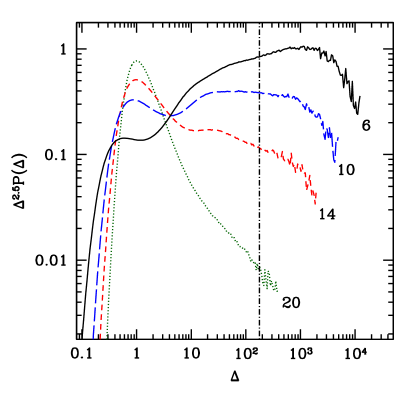
Figure 2.— Gas PDFs for our fiducial simulation B2 ($512^{3}$, 0.5 Mpc) at different redshifts, as labelled beside the curves. The vertical dot-dashed line delineates the overdensity $\Delta_{\rm vir}=18\pi^{2}$ of a virialized isothermal sphere. If collapsed structures have a density profile of the form $\rho\propto r^{-2}$, for $\Delta_{\rm vir}<\rho/\bar{\rho}<\Delta_{\rm max}$, then $P(\Delta)\propto\Delta^{-2.5}$ for $\Delta_{\rm vir}<\Delta<\Delta_{\rm max}$. We plot the PDF multiplied by $\Delta^{2.5}$ so that the curve should approach a constant for $\Delta>\Delta_{\rm vir}$ if gas is collapsed within these structures.

2.2. Post-processed Ionization Calculation

In order to simulate the effects of self-shielding by absorption systems, we postprocess the SPH density field with a multifrequency radiative transfer algorithm. This involves tracing the attenuation of the ionizing radiation along different lines of sight throughout the volume while assuming photoionization equilibrium.

2.2.1 Ultraviolet Background Spectrum

We consider a background ionizing intensity $I_{\nu}$, so that the flux of photons capable of ionizing hydrogen is

$$F=\int d\Omega\int_{\nu_{HI}}^{4\nu_{HI}}\frac{I_{\nu}}{h\nu}d\nu,$$ (1)

where $h\nu_{HI}=13.6$ eV is the photon energy at the Lyman edge. The upper limit in the integral corresponds to the ionizing threshold for fully ionizing helium – we assume helium is singly ionized along with hydrogen, and therefore only consider photons below the He II Lyman edge.

We adopt a power-law UVB spectrum,

$$I_{\nu}=I_{o}\left(\frac{\nu}{\nu_{HI}}\right)^{-\alpha},$$ (2)

where $\nu_{HI}\leq\nu\leq 4\nu_{HI}$ and $I_{o}$ is the intensity at the Lyman edge. In our analysis we have sampled a region of parameter space for which $1\leq\alpha\leq 3$. Our fiducial value of $\alpha=2$ is chosen to be consistent with the spectral index we would expect for an ionizing background produced from a mixture of galaxies and quasars (e.g., Bolton & Haehnelt, 2007). Our results exhibit only a minor dependence on spectral index in this range, as also found by McQuinn et al. (2011). For this reason we henceforth refer only to our fiducial case of $\alpha=2$.

The intensity is often expressed in terms of the quantity $J_{-21}$, defined to be the isotropic equivalent of $I_{o}$, $(\int I_{0}d\Omega)/(4\pi)$, in units of $10^{-21}\ {\rm erg}\ {\rm cm}^{-2}{\rm s}^{-1}{\rm Hz}^{-1}{\rm ster}^{-1}$. For the form expressed in equation (2), we can integrate equation (1) to relate $J_{-21}$ to the flux of ionizing photons. For $\alpha=2$, we obtain:

$$J_{-21}=0.09\left(\frac{F}{10^{5}\ {\rm cm}^{-2}{\rm s}^{-1}}\right).$$ (3)

Another useful quantity to describe the UVB is $\Gamma_{-12}$, defined to be the ionization rate per atom, in units of $10^{-12}\ {\rm s}^{-1}$:

$$\Gamma_{-12}=0.3\left(\frac{F}{10^{5}\ {\rm cm}^{-2}{\rm s}^{-1}}\right).$$ (4)

Note that this refers to the ionization rate corresponding to a given background, and not the mean ionization rate per atom along our rays, which is lower due to attenuation and includes the neutral component of the IGM.

We calculate the ionization state of the volume for a broad range of background flux with the fiducial value of $F=10^{5}\ {\rm cm}^{-2}{\rm s}^{-1}$ taken to be consistent with the value of $\Gamma_{-12}\sim 0.3$ inferred from the optical depth of the Ly$\alpha$ forest seen in quasar spectra (e.g., Bolton & Haehnelt, 2007). Due to its common usage in the literature, we will report our results in terms of $\Gamma_{-12}$, though it should be remembered that its conversion to flux simply follows equation (4).

2.2.2 Ray-tracing

In our ray-based approach, the UVB has a plane-parallel direction dependence, so that $I_{\nu}=F_{\nu}\delta(\hat{n})$, where $\hat{n}$ is the direction of propagation of the radiation and $F_{\nu}$ is the spectral flux density. This is appropriate especially in the beginning stages of reionization, where a given patch of the IGM is initially exposed to a one-sided flux from the downstream direction of the ionization front. In addition, we use the “case B” recombination coefficient which assumes that recombinations to the ground state are quickly canceled by subsequent photoionizations and implies that rays can be treated independently. In reality, ionizing radiation produced by recombinations directly to the ground state becomes part of the UVB, changing the spectral shape that we adopt in equation (2), but not the total ionizing photon flux. Given the relative insensitivity we find to the spectral shape, using case B recombination rates should be a good approximation. Finally, because the equilibration time is very short compared to the Hubble time, we use photoionization equilibrium, which allows us to calculate the ionization state and attenuation of the background self-consistently by sequentially iterating along the ray in the direction $\hat{n}$.

To obtain an unbiased sample of the gas density field and minimize noise, the rays are assigned starting points uniformly distributed in a plane with orientations perpendicular to the plane. We use three orthogonal planes in order to sample different directions. Each ray segment corresponds to a cubic volume element, within which the mean density is obtained from the SPH particle data by the mass-conserving spline interpolation outlined in Alvarez et al. (2006). The ray segments have lengths given by $L/N_{\rm ray}$, where $L$ is the box size, so that the number of rays is proportional to $N_{\rm ray}^{2}$, while the number of segments along a given ray is proportional to $N_{\rm ray}$. We check for convergence in our radiative transfer calculations by interpolating to a variety of values for $N_{\rm ray}$. From this we find that it is necessary to interpolate to $N_{\rm ray}=1024$ for the $256^{3}$ and $512^{3}$ particle simulations and to $N_{\rm ray}=2048$ for the $1024^{3}$ particle simulations.

2.2.3 Equilibirum Radiative Transfer

The equation of radiative transfer for $I_{\nu}$ is

$$\frac{dI_{\nu}}{ds}=-n_{\rm HI}{\sigma_{\nu}}I_{\nu}+\epsilon_{\nu},$$ (5)

where $s$ is the proper distance and $n_{\rm HI}$ is the proper number density of neutral hydrogen. Here we are concerned with the transfer of ionizing radiation through a patch of IGM in which there are no sources, and therefore set $\epsilon_{\nu}=0$.

The ionization rate within a given ray segment is related to the background intensity and neutral hydrogen column density, $N_{HI}$, integrated along a given ray by using the solution of equation (5):

$$\Gamma=4\pi\int_{\nu_{HI}}^{4\nu_{HI}}\frac{I_{\nu}}{h\nu}\sigma_{\nu}e^{-N_{HI}\sigma_{\nu}}d\nu,$$ (6)

where $\sigma_{\nu}$ is the absorption cross section, with mean value

$$\bar{\sigma}\equiv\frac{\int_{\nu_{HI}}^{4\nu_{HI}}\sigma_{\nu}\frac{I_{\nu}}{h\nu}d\nu}{\int_{\nu_{HI}}^{4\nu_{HI}}\frac{I_{\nu}}{h\nu}d\nu}=2.84\times 10^{-18}~{}{\rm cm^{2}}.$$ (7)

The flux of ionizing photons is diminished along the ray through absorption by intervening neutral hydrogen, and the spectrum steepens as softer photons are preferentially absorbed.

To determine the opacity along the ray self-consistently, we iterate along the ray, using the total H I column density from the previous ray segments to calculate the photoionization rate at the current segment using equation (6). This is then used to determine the neutral hydrogen density in the current segment under the assumption of photoionization equilibrium:

$$\Gamma n_{HI}=\alpha_{B}n_{HII}n_{e},$$ (8)

where $n_{HI}$, $n_{HII}$ and $n_{e}$ are the number densities of neutral hydrogen, ionized hydrogen, and electrons within that segment. The resulting value of H I density is then used to update the total column density, and the procedure is repeated until the end of the ray is reached.

Equation (8) assumes a uniform radiation field within each ray segment. This assumption breaks down if the segment becomes sufficiently optically thick that $\Gamma$ changes significantly across it. To address this issue, individual ray segments are split into plane-parallel subsegments in the direction $\hat{n}$ with widths chosen such that the flux passing through each subsegment is attenuated by no more than $2\%$ of its initial value. Photoionization equilibrium is applied in sequence to each subsegment and global quantities pertaining to the segment as a whole are computed as volume averages over each subsegment.

We assume that all free electrons within the volume come from hydrogen and consider a uniform gas temperature of $T_{\rm gas}=10^{4}$ K so that $\alpha_{B}=2.6\times 10^{-13}\ {\rm cm}^{3}{\rm s}^{-1}$. Including helium in our calculations would lead to small corrections in the hardening of the radiation at high optical depths, due to the slightly different frequency dependence of the He I absorption cross-section relative to that of H I. Given the insensitivity of our results to varying the spectral slope $\alpha$, inclusion of helium radiative transfer would not improve the accuracy of our results, while needlessly complicating their interpretation, so we neglect it.

2.2.4 Optimal Ray Length and the Mean Free Path

The opacity of the IGM can be written in terms of the mean free path, with the equation of transfer for the flux of ionizing photons given by

$$\frac{dF}{ds}=-\frac{F(1+z)}{\lambda},$$ (9)

where $F$ is the total flux of ionizing photons in units of cm^-2s^-1, and the factor $1+z$ accounts for the fact that we define the mean free path to be in comoving units, and is the definition we use throughout this paper. We calculate the mean free path along a given ray as the solution to equation (9):

$$\lambda=-\frac{s}{{\rm ln}(F_{\rm out}/F)},$$ (10)

where $s$ is now the comoving length of the ray, $F$ is the incident flux at the start of the ray, and $F_{\rm out}$ is the attenuated flux leaving the last ray segment. The total mean free path is determined by first averaging $F_{\rm out}$ over all rays, then applying equation (10).

Naively, we may choose to set $s=L$ so that each ray samples the entire length of the box. However, we must be careful since the use of equation (10) is not physically meaningful in the optically thick limit where $F_{\rm out}$ can tend to 0. In other words, we want to determine the opacity of the IGM due to small-scale structure at a fixed background flux, but including the cumulative effect of this shielding over distances approaching the mean free path would correspond to a lower flux than what we assume.

An easy way to avoid this problem is to send photons along shorter rays. Of course, this has the disadvantage of sampling smaller portions of the IGM, possibly missing individual self-shielded structures. It is thus optimal to choose a ray length such that the rays on average remain optically thin, while still sampling a sufficiently long distance to take into account the self-shielding of individual dense structures. We achieve this by first calculating $\lambda$ as a function of $s$, and then choose the optimal ray length to be the largest value of $s$ for which $s\leq\lambda(s)/5$. A lower cutoff of $s\geq L/32$ is also applied. If this condition cannot be satisfied we flag the given region of parameter space and omit its inclusion in our analysis. For ray lengths $s<L$, the usage of the box is maximized by resetting the intensity along each ray after a distance of $s$, until the ray has traversed a distance $L$.

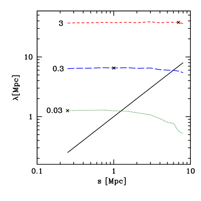
Figure 3.— Here we demonstrate our procedure for choosing the optimal ray length that adequately samples the IGM while remaining optically thin. The data pertains to simulation B6 ($512^{3}$, 8 Mpc) taken at redshift $z=10$. The nearly horizontal lines show $\lambda$ as a function of ray length $s$ for different photoionization rates where the labels denote $\Gamma_{-12}$ in units of $10^{-12}\ {\rm s}^{-1}$. For each of these lines, the optimal ray length is chosen as the largest value of $s$ for which $s\leq\lambda(s)/5$ and is denoted by a black cross. For comparison, the diagonal line traces out $\lambda=s$ so that portions rightward of this curve belong to the optically thick regime where the mean free path changes significantly.

Figure 3 demonstrates our procedure of selecting ray lengths at different fluxes for simulation B6 at $z=10$. The mean free path converges in the optically thin limit where $\lambda\gtrsim s$ but begins to deviate strongly during the transition to the optically thick transition when $\lambda$ approaches $s$. It is clear from the plot that an erroneous value for $\lambda$ would be obtained for an improper choice of $s$. The convergence of $\lambda$ in the optically thin limit shows that our choice of picking $s$ to be bounded by $\lambda/5$ is robust in changing this fraction by a factor of a few.

3. Simulation Results

We first describe the dependence of clumping factor, $c_{l}$, of ionized gas on redshift and photoionization rate. Next, we use the gas PDF matched to the clumping factors we have obtained, to define a critical overdensity, $\Delta_{\rm crit}$, above which gas remains self-shielded and neutral. The opacity of the IGM to ionizing radiation, expressed in terms of the mean free path, $\lambda$, is described next. We first discuss its overall properties and then show how it can be used to relate the emissivity of ionizing sources to the photoionizing background that they produce. Finally, we compare the clumping factors and mean free paths obtained here to those which would be expected for an optically thin model of the IGM.

The main goal of this work is to assess the small-scale convergence of numerical quantities during the initial phase of reionization. This is presented in $\S$4 where we show simulation C3 ($1024^{3}$, 1 Mpc) to be our “converged” simulation. However, since C3 was only evolved to $z=10$, we show here results from our fiducial simulation B2 ($512^{3}$, 0.5 Mpc) in order to present results down to $z=6$. Table LABEL:table:datapts2 summarizes the clumping factors, critical overdensities, and mean free paths at select redshifts and photoionization rates for simulation B2. These values are within $6\%$ of those from the converged simulation C3 for all $z\geq 10$.

3.1. Clumping Factor

Studies of reionization typically make use of the clumping factor of ionized gas, defined as

$$c_{l}\equiv\langle n_{e}^{2}\rangle/\langle n_{e}\rangle^{2},$$ (11)

where $n_{e}$ is the number density of free elections and angled brackets denote volume averages over space. The clumping factor describes the enhancement of the recombination rate relative to a uniform gas distribution, and is therefore crucial in understanding the role of inhomogeneities in the ionizing photon budget during and after reionization.

Before proceeding to discuss the clumping factors obtained here, it is first useful to make some comments regarding the form of equation (11). This equation involves a volume average over the free electron density in each ray segment of the box without applying any density cutoffs in considering which electrons contribute to recombinations within the IGM. We have made this choice to facilitate the use of equation (12) which allows us to determine the critical overdensity required for self-shielding within a patch of the IGM that does not contain any reionizing sources. This can then be applied in studies that simulate self-shielding by turning off an optically thin flux above a threshold overdensity. Another choice would be to compute the clumping factor based only on gas with overdensity below some cutoff that is assumed to represent the maximum density for which recombinations occur within the IGM. This is ideal for the scenario where one is interested in separating recombinations occurring within the IGM from those occurring within the interstellar medium (ISM) of ionizing sources. The latter can be accounted for through the use of an escape fraction describing the fraction of ionizing photons that escape the ISM of reionizing sources into the surrounding IGM. It is important to note that the numerical value obtained for the clumping factor depends on the particular definition that is used. Regardless, the convergence tests described in $\S$4, which are based on the clumping factor described above, remain robust to whatever definition of clumping factor is assumed. For more detailed discussions of the clumping factor and comparisons between different definitions we refer the reader to the recent works of Shull et al. (2012) and Finlator et al. (2012).

We now proceed to discuss the clumping factor obtained from the radiative transfer calculations performed on our fiducial simulation B2. This is shown in Figure 4 where we plot $c_{l}$ for a variety of redshifts and fluxes. Some general trends of the clumping factor are shown by comparing the two panels of this figure. In the first place, at fixed photoionization rate, $c_{l}$ increases with decreasing redshift which is consistent with ongoing structure formation within the IGM. Furthermore, at fixed redshift, $c_{l}$ increases with the strength of the ionizing background as the flux of ionizing photons are able to penetrate further into thick gas clouds, exposing their dense interiors where the recombination rate is greatest. Eventually, at large enough flux of $\Gamma_{-12}\gtrsim 1000$, the clumping factor plateaus as the ionization state of the box saturates and all the gas has been ionized. At this point $c_{l}$ tends to the total clumping factor of gas in the box as $n_{e}$ approaches $n$.

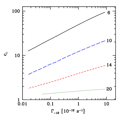
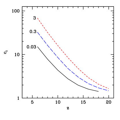
Figure 4.— (left) Clumping factor versus photoionization rate $\Gamma_{-12}$ in units of $10^{-12}~{}{\rm s}^{-1}$ for different redshifts, as labelled beside the curves. (right) Clumping factor versus redshift for different photoionization rates with labels denoting the value of $\Gamma_{-12}$. In both cases the data pertains to our fiducial simulation B2 ($512^{3}$, 0.5 Mpc) and regions of parameter space ($z>18$ and $\Gamma_{-12}<0.05$) that do not satisfy the ray length criterion described in $\S 2.2.4$ are omitted.

Historically, clumping factors of $c_{l}\sim 30$ at $z\sim 6$ have been found to be appropriate (e.g., Gnedin & Ostriker, 1997), though more recently there has been a growing trend towards values an order of magnitude smaller. It thus appears contrary to historical development that we reproduce $c_{l}\sim 30$ at $z=6$ with our fiducial case of $\Gamma_{-12}=0.3$, and find even larger values with increased flux. However, as explained by Pawlik et al. (2009), the passage of an ionization front through the IGM will photoevaporate the smallest halos in the box and consequently suppress the evolution of the clumping factor at small scales as the gas is dispersed back into the diffuse IGM. Since we do not include such hydrodynamic feedback processes in our analysis, the values reported here cannot be used in reference to an IGM that has been heated through photoionization. Nevertheless, our values are perfectly applicable to the early stages of reionization, before the gas has had time to respond to the ionizing radiation field. Moreover, as discussed in $\S 5$, previous simulations have underestimated the clumping factor by a factor of $\sim 3$ during this period, and may therefore be underestimating its subsequent evolution and the impact that unresolved small-scale structure had in regulating the early stages of reionization.

Table 2Opacity of the Unheated IGM at Select Values

z	$\Gamma_{-12}$ $[10^{-12}\ {\rm s}^{-1}]$	$c_{l}$	$\Delta_{\rm crit}$	$n_{\rm crit}$ [cm-3]	$\lambda$ [Mpc]
18	0.03	1.4	6.1	0.008	0.1
14	0.03	2.0	14	0.009	0.3
10	0.03	4.4	34	0.008	0.7
8	0.03	7.8	55	0.007	1.1
6	0.03	15	100	0.006	2.1
18	0.3	1.7	25	0.031	0.9
14	0.3	3.0	52	0.032	1.6
10	0.3	8.6	120	0.029	3.0
8	0.3	16	200	0.027	4.5
6	0.3	33	390	0.025	8.3
18	3	2.1	110	0.14	7.1
14	3	4.8	210	0.13	10
10	3	16	470	0.11	15
8	3	32	760	0.10	21
6	3	68	1400	0.09	36

3.2. Critical Overdensity for Ionization

Since the clumping factor describes the distribution of ionized gas within the volume, it is in principle derivable from knowledge of the gas PDF and details of the photoionizing radiation field. In a simplified description, we assume that all gas within the box with overdensity $\Delta<\Delta_{\rm crit}$ is ionized, while the rest is neutral. This is obviously an idealized description of reality where a gradual transition between ionized and neutral regions will necessarily occur. Any departures from the simplified model reflect variations in the local ionizing background and degree of self-shielding and shadowing within the inhomogeneous IGM (Miralda-Escudé et al., 2000).

In the simplified model the clumping factor of ionized gas is related to the total gas PDF through the following expression:

$$c_{l}=\frac{\int_{0}^{\Delta_{\rm{crit}}}\Delta^{2}P(\Delta)\ d\Delta}{\left(\int_{0}^{\Delta_{\rm{crit}}}\Delta P(\Delta)\ d\Delta\right)^{2}},$$ (12)

where $\Delta_{\rm{crit}}$ is interpreted as the critical overdensity above which self-shielding prevents the gas from becoming ionized. It is often useful to assume the form of equation (12) taken with some nominal choice for $\Delta_{\rm crit}$ in order to compute $c_{l}$ from a given gas PDF. For example, Chiu et al. (2003) consider a model where all gas within collapsed halos is self-shielded while all remaining gas is subject to ionization from an UVB. In this case, $\Delta_{\rm crit}=6\pi^{2}$ corresponding to the overdensity at the virial radius of an isothermal sphere with a mean overdensity of $\Delta_{\rm vir}=18\pi^{2}$.

Since we compute the clumping factor directly from our radiative transfer calculations, we take the opposite approach, inverting equation (12) in order to compute $\Delta_{\rm crit}$ from knowledge of $P(\Delta)$ and $c_{l}$. In doing so, we observe the expected trend that $\Delta_{\rm crit}$ increases when the photoionization rate is increased, making the medium more susceptible to ionization. In fact, we find the rough proportionality $\Delta_{\rm crit}\propto\Gamma_{-12}^{2/3}$ which, from equation (4) of McQuinn et al. (2011), is expected for a PDF satisfying $P(\Delta)\propto\Delta^{-2.5}$. We showed in Figure 2 that our PDFs satisfy this power-law at $z\lesssim 10$ for $\Delta>\Delta_{\rm vir}$. This is consistent with the model where gas at these densities is collapsed in isothermal spheres. Around our fiducial value of $\Gamma_{-12}=0.3$, we further find that $\Delta_{\rm crit}$ is roughly proportional to $(1+z)^{-3}$, indicating that the critical proper hydrogen number density, $n_{\rm crit}$, is rather insensitive to redshift. A good value to take is $n_{\rm crit}\sim 0.1$ cm${}^{-3}~{}\Gamma_{-12}^{2/3}$.

The validity of the idealized model where all gas with overdensity $\Delta<\Delta_{\rm crit}$ is ionized is tested in Figure 6. Here we plot the total gas PDF along with the ionized and neutral PDFs obtained from our radiative transfer calculation using our fiducial parameters $\Gamma_{-12}=0.3$ and $z=10$ for simulation B2. The vertical dot-dashed line shows the corresponding value of $\Delta_{\rm crit}$ – its role in delineating the neutral and ionized portions of the gas is clearly visible. As anticipated, the transition between ionized and neutral regions is not sharp, but rather gradual as a consequence of the spatially varying ionizing background and self-shielding due to dense gas pockets. Nevertheless, our findings indicate that the approximation that $\Delta_{\rm crit}$ represents the critical overdensity above which self-shielding maintains the neutral state of the IGM is generally a good one.

3.3. Mean Free Path

We quantify the opacity of the IGM to the exposed UVB through the use of the mean free path of ionizing radiation. Conceptually, one can consider the mean free path to be affected by two components: a diffuse gaseous phase that pervades the IGM and thick gas clouds embedded within collapsed dark matter halos. The latter make up a significant fraction of absorption systems that have neutral hydrogen column densities $N_{HI}\gtrsim 1/\bar{\sigma}\approx 10^{17}\ {\rm cm}^{2}$ allowing them to self-shield against ionizing radiation. It is within these optically-thick structures where the global recombination rate of the IGM is dominated and the majority of ionizing photons are absorbed (Miralda-Escudé et al., 2000). As a result, they can significantly impede the progress of reionization.

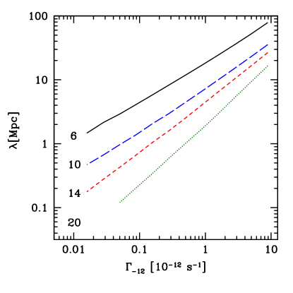
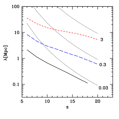
Figure 5.— (left) The mean fee path versus photoionization rate $\Gamma_{-12}$ in units of $10^{-12}~{}{\rm s}^{-1}$ for different redshifts, as labelled. (right) Mean free path versus redshift for different photoionization rates with labels indicating the value of $\Gamma_{-12}$. In both cases the data pertains to our fiducial simulation B2 ($512^{3}$, 0.5 Mpc) and regions of parameter space ($z>18$ and $\Gamma_{-12}<0.05$) that do not satisfy the ray length criterion described in $\S 2.2.4$ are omitted. The dotted black curves in the right panel show the mean free path expected for an optically thin, completely ionized, and homogeneous IGM as expressed in equation (17). From bottom to top in the plot, the dotted lines take $\Gamma_{-12}=0.03$, $0.3$, and $3$, and are each calculated using $x=c_{l}=1$. We expect the dotted lines to converge with our results at high redshift when the medium approaches homogeneity. At low redshift we observe a large suppression in the calculated mean free path that results from increased structure formation within the inhomogeneous IGM.

The mean free path obtained from our radiative transfer calculations is computed through the use of equation (10) which naturally encompasses both the clumpy IGM and halo components. In Figure 5 we plot the mean free path as a function of photoionization rate for fixed redshift and also as a function of redshift for fixed photoionization rate. Some general trends are immediately clear in this plot. In the first place, at fixed redshift we see that the mean free path increases with the strength of the ionizing background. A stronger flux of ionizing photons will naturally penetrate further through a diffuse IGM and overcome thicker self-shielding structures, consistent with the previous observation that $\Delta_{\rm crit}\propto\Gamma_{-12}^{2/3}$. In addition, when the ionizing background is held constant, the mean free path is found to increase with decreasing redshift.

It is important to note that there are two competing factors affecting the redshift evolution of $\lambda$. On the one hand, the expansion of the Universe continually dilutes the density of hydrogen, hence favouring a strong increase in $\lambda$ with decreasing $z$. On the other hand, increased structure formation at low redshift enhances the distribution of Lyman-limit systems that strongly inhibit the distance an ionizing photon can propagate through the IGM before being absorbed. In the right panel of Figure 5 we compare $\lambda$ obtained here to equation (17) for the same set of photoionization rates. Taking $x=c_{l}=1$ in this equation yields the mean free path we would obtain in an optically thin, homogeneous, and completely ionized medium. In such a model the mean free path evolves rapidly with redshift as $\lambda\propto(1+z)^{-5}$. Instead, we observe a strong suppression in mean free path at low redshift compared to equation (17). This highlights the important contribution from inhomogeneities in the IGM.

3.4. Relationship Between Emissivity and Photoionization Rate

In the context of reionization it is desirable to know the ionizing background produced by some population of sources with known emissivity. This relationship can be found by solving

$$\Gamma=\dot{n}_{\rm ion}(1+z)^{2}\lambda(\Gamma,z)\bar{\sigma},$$ (13)

where $\dot{n}_{\rm ion}$ is the comoving ionizing emissivity and $\lambda(\Gamma,z)$ is the comoving mean free path that depends on both the ionizing background and redshift. In Figure 7 we show the dependence of $\Gamma$ on $\dot{n}_{\rm ion}$ by solving equation (13) with the mean free paths taken from our radiative transfer calculations. We find that $\Gamma$ exhibits a rather steep dependence on emissivity and appears to diverge at large values of $\dot{n}_{\rm ion}$. This behaviour is attributed to the fact that not only are there more ionizing photons as the emissivity rises, but also their ability to penetrate further through the IGM increases.

Table 3Power law index of $\Gamma\propto\dot{n}_{\rm ion}^{\gamma}$

	z
	6	8	10	12	14	16	18	20
$\gamma$	2.6	2.9	3.1	3.7	4.5	6.7	10	14

We can relate this behaviour back to the dependency of $\lambda$ on $\Gamma$. For instance, suppose we have the simple relation $\lambda\propto\Gamma^{\beta}$ at some redshift. Then from equation (13) we will have that $\Gamma\propto\dot{n}_{\rm ion}^{\gamma}$ where $\gamma=(1-\beta)^{-1}$. In Table 3 we list the values of $\gamma$ obtained by fitting a power-law to our fiducial mean free paths within the range $0.1\leq\Gamma_{-12}\leq 1$ at different redshifts. This flux range is considered to emphasize the relationship between $\Gamma$ and $\dot{n}_{\rm ion}$ around our fiducial value of $\Gamma_{-12}=0.3$. We find that the relationship between $\Gamma$ and $\dot{n}_{\rm ion}$ strengthens as the redshift increases – $\gamma$ varies from 2.6 to 14 between redshifts 6 and 20 respectively. This occurs because the slope $\beta$ rises as the IGM becomes more uniform, approaching a limiting value of unity for a completely homogeneous Universe with $c_{l}=1$ in equation (17) – a manifestation of “Olber’s Paradox”.

From this trend we can deduce that decreasing the simulation resolution should steepen the curves in Figure 7 as the density distribution becomes more homogenous. Indeed, this relation is observed between our suite of simulations where we find $\gamma=3.2$ at $z=6$ for our worst-resolved simulation A6 ($256^{3}$, 8 Mpc), compared to $\gamma=2.6$ for simulation B2. McQuinn et al. (2011) report the value of $\gamma\sim 4$ at $z=6$. The discrepancy with our result likely arises from a combination of our increased resolution and our omission of photoheating which would suppress accretion of gas onto low-mass halos and promote homogeneity.

The photoionization rate after reionization can be derived from measurements of the Ly$\alpha$ forest. This was done by Kuhlen & Faucher-Giguère (2012) who list the values of $\Gamma$ and $\dot{n}_{\rm ion}$ for redshifts between 2 and 6. The quoted values at $z=6$ are $\Gamma_{-12}<0.19$ and $\dot{n}_{\rm ion}<2.6\times 10^{50}~{}{\rm s^{-1}~{}Mpc^{-3}}$. Looking at Figure 7 we see that our $z=6$ curve predicts an emissivity an order of magnitude too large when $\Gamma_{-12}=0.19$. As we discuss in $\S 5$, our results at $z\lesssim 10$ are hindered by the omission of radiative feedback that would otherwise smooth inhomogeneities on small scales. Photoheating suppresses structure growth within the IGM thereby increasing the mean free path at fixed conditions as ionizing photons travel further before encountering an optically thick absorption system. From equation (13) a larger mean free path produces a higher ionization rate at fixed emissivity, implying that the $z=6$ curve in Figure 7 would shift upwards in the presence of heating. If this shift were to bring us into agreement with observations we would require that our calculated mean free path at $\Gamma_{-12}=0.19$ increase by an order of magnitude to allow for an order of magnitude reduction in the emissivity required to produce such a background. In Figure 5 we find $\lambda\approx 7$ Mpc at $z=6$ for $\Gamma_{-12}=0.19$. This means that a mean free path of 70 Mpc would be required in a heated IGM to bring us into agreement with observations of the Ly$\alpha$ forest. This is in reasonable agreement with the value of $\lambda=49\pm 14$ Mpc reported by Kuhlen & Faucher-Giguère (2012) as the mean free path at the Lyman edge. Note that at redshifts $z\gtrsim 10$, before photoheating is important, the curves in Figure 7 should be correct. Of course, reionization becomes patchy at high redshift, making a description in terms of an IGM with a single UVB flux and mean free path less accurate.

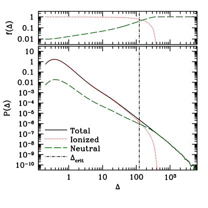
Figure 6.— The bottom panel compares the total gas PDF of our fiducial simulation B2 ($512^{3}$, 0.5 Mpc) to the PDFs of neutral and ionized gas within the box after radiative transfer is applied. Ray segments are labelled as ionized if they have an ionized fraction greater than 0.5 and are labelled neutral otherwise. The data corresponds to a snapshot at $z=10$ with an ionizing background of $\Gamma_{-12}=0.3$. The vertical dot-dashed line denotes $\Delta_{\rm crit}$ determined by comparing $c_{l}$ obtained from the radiative transfer calculation to the total gas PDF through equation (12). The top panel shows the corresponding volume fraction of neutral and ionized gas as a function of $\Delta$.

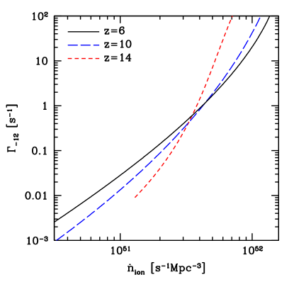
Figure 7.— The photoionization rate, expressed in terms of $\Gamma_{-12}$, as a function of the comoving ionizing emissivity at different redshifts. These curves are evaluated by solving equation (13) using $\lambda(\Gamma,z)$ obtained from our radiative transfer calculations performed on our fiducial simulation B2 ($512^{3}$, 0.5 Mpc). At low flux we truncate the $z=14$ curve when it enters the optically thick domain where it no longer satisfies the ray length criterion described in $\S 2.2.4$.

The strong scaling relations observed here suggest that small changes in $\dot{n}_{\rm ion}$ can boost $\Gamma$ by substantial amounts. McQuinn et al. (2011) use this to argue that the rapid evolution in $\Gamma$ observed by Fan et al. (2006) at $z\approx 6$ can be explained by a small change in the emissivity of the ionizing background rather than attributing this effect to the overlap phase of reionization.

3.5. Relationship Between Mean Free Path and Clumping Factor

Suppose there is an infinitesimally thin slab of width $ds$ whose area element $dA$ is exposed to some flux $F$. In ionization equilibrium, the number of ionizations occurring per unit time balance the number of recombinations:

$$dFdA=\alpha_{B}n_{e}n_{HII}dAds,$$ (14)

where $dF$ is the attenuation of flux passing through the slab. Dividing both sides of this expression by $dAds$, substituting equation (9), and taking $n_{e}=n_{HII}$ implies

$$F(1+z)/\lambda=\alpha_{\rm B}n_{e}^{2}.$$ (15)

Finally, taking the clumping factor defined in equation (11) and the ionized fraction $x\equiv\langle n_{e}\rangle/\langle n_{H}\rangle$ we obtain:

$$F(1+z)/\lambda=c_{l}\alpha_{\rm B}x^{2}\langle n_{H}\rangle^{2}.$$ (16)

For an ionized gas temperature of $T_{\rm gas}=10^{4}$ K,

$$\lambda\simeq\frac{23~{}{\rm Mpc}}{x^{2}c_{l}}\left(\frac{\Gamma_{-12}}{0.3~{}10^{-12}~{}{\rm s}^{-1}}\right)\left(\frac{1+z}{11}\right)^{-5},$$ (17)

where we have made use of equation (4) for the conversion from flux to photoionization rate.

In Figure 8 we plot $c_{l}$ versus $\lambda$ and $x^{2}c_{l}$ versus $\lambda$ from our radiative transfer calculations at $z=10$ with $\Gamma_{-12}=0.3$ for each of the simulations listed in Table LABEL:table:simparams. In each panel the dotted line traces equation (17) that we would expect for an optically thin IGM exposed to the given flux. The overall agreement between $\lambda$ and the simulation points in the bottom panel indicates consistency in the definition of the mean free path and detailed balance between absorptions and ionizations. The minor deviations between the data points and the dotted curve arise because our rays have a finite length, $s$, so the mean free path evaluated in equation (17) will not correspond exactly to equation (10), which is strictly correct only in the limit where $s\longrightarrow 0$.

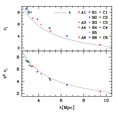
Figure 8.— $c_{l}$ versus $\lambda$ (top panel) and $x^{2}c_{l}$ versus $\lambda$ (bottom panel) for all simulations taken at $z=10$ with a photoionization rate $\Gamma_{-12}=0.3$. In each panel points denote simulation values according to the legend in the top right corner of the plot. Traced by the dotted line is equation (17) which describes the relationship between mean free path and clumping factor for an optically thin IGM.

The simulations span a large range of values in Figure 8 with $c_{l}$ ranging from 2.6 to 8.8 and $\lambda$ from 2.9 to 9.5 Mpc. This spread arises from the broad variation in spatial and mass resolution exhibited by the suite of simulations. In spite of this, there is a clear grouping of points at $c_{l}\sim 8$ and $\lambda\sim 3$ Mpc. This reflects the trend towards numerically converging to the “correct” clumping factor and mean free path and is our next topic of focus.

4. Numerical Convergence

In this section, we attempt to answer the following question: What mass resolution and box sizes are necessary in cosmological hydrodynamics simulations, in order to obtain accurate results for the inhomogeneity of an unheated IGM? Clearly, simulations must have sufficient mass resolution to resolve the internal structure of the lowest mass halos that can contain gas. In addition, however, such simulations must cover a large enough volume to contain a representative sample of the low-mass halos that dominate the opacity of the IGM.

In Figure 9 we plot the clumping factors and mean free paths obtained from the radiative transfer calculations performed on each of the simulations listed in Table LABEL:table:simparams. To obtain a picture of convergence we display how $c_{l}$ and $\lambda$ vary as functions of simulation box size, $L$, (left panels) and dark matter particle mass, $m_{\rm dm}$, (right panels) for our fiducial redshift $z=10$ and photoionization rate $\Gamma_{-12}=0.3$. Though the discussion below pertains explicitly to these fiducial values we have checked that the picture remains consistent for $10\leq z\leq 20$ and $0.01\leq\Gamma_{-12}\leq 10$.

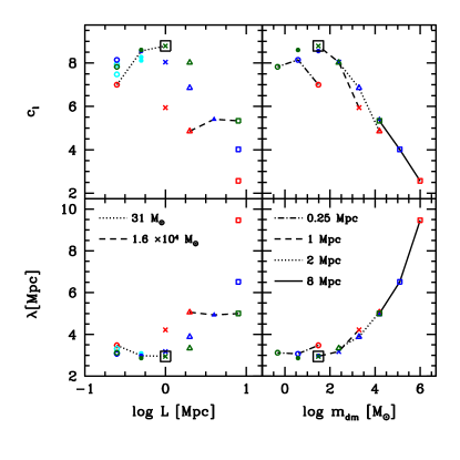
Figure 9.— Clumping factor and mean free path versus simulation box size (left panels) and dark matter particle mass (right panels) for $z=10$ and $\Gamma_{-12}=0.3$. In each panel point types distinguish between different simulations and follow the legend in Figure 8. Lines in the left panels connect simulations with fixed particle mass, while lines in the right panels connect simulations with fixed volume. The converged simulation C3 ($1024^{3}$, 1 Mpc) is denoted by a green cross and is highlighted by a black square for easy identification. In the two left panels, open cyan circles and closed cyan circles denote the values of $c_{l}$ and $\lambda$ obtained from different random realizations of simulations B1 and B2 respectively.

Starting in the top right panel of Figure 9 we show how $c_{l}$ changes as the mass resolution of the simulations is varied. As expected, the clumping factor increases as the resolution is refined and begins to plateau to a common value of $c_{l}\sim 8.8$ at $m_{\rm dm}\sim 30~{}M_{\odot}$, when a sufficiently low particle mass required to resolve the smallest gaseous structures in the box is reached. Simulations with larger particle mass are unable to resolve the smallest inhomogeneities contributing to the clumpiness of the IGM and consequently imply clumping factors up to a few times smaller than the converged result. In the opposite limit we find that simulations with $m_{\rm dm}<5~{}M_{\odot}$ are also yielding smaller clumping factors of $c_{l}\sim 8$. This appears counterintuitive at first glance since these simulations should have no problem resolving the Jeans scale of the IGM. However, their inability to converge on $c_{l}$ is attributed to their small box size, as explained below. The three smallest simulations with $L=0.25$ Mpc are connected by a dot-dashed line and all display conspicuously unconverged values.

The dependence of clumping factor on box size is shown in the top left panel of Figure 9. In this case we expect to find a minimum box size above which simulations converge on $c_{l}$. Smaller boxes fail to capture power from large-scale modes and should therefore have reduced clumping factors. Larger boxes that are able to capture a representative collection of absorption systems within their volume should converge provided that they have sufficient mass resolution. These general trends can be identified by the behaviour shown in the top left panel of Figure 9. There is a clear convergence of points near $L\sim 1$ Mpc and $c_{l}\sim 8.8$ with $c_{l}$ falling off on either side. Simulations with $L\lesssim 1$ Mpc have insufficient volumes to converge with this result, while those with $L\gtrsim 1$ Mpc have insufficient mass resolutions. Convergence occurs in the middle ground where both a sufficient volume and mass resolution are attained.

We find similar behaviour by comparing how $\lambda$ changes between simulations. From the bottom panels of Figure 9 we see that the resultant behaviour is essentially an inversion of that described for $c_{l}$. Firstly, simulations with coarse mass resolutions overestimate $\lambda$. These runs are unable to resolve small-scale inhomogeneities and the degree of self-shielding that would otherwise inhibit the propagation of ionizing photons through neutral patches of the IGM. Secondly, the smallest boxes also produce values of $\lambda$ that are too large. As mentioned above, these simulations underproduce the collection of halos that shield against the propagation of an ionization front through the IGM.

The simulations shown here have relatively small volumes in a cosmological context. One issue that must be considered with these small boxes is that of sample variance. In the left panels of Figure 9 we plot $c_{l}$ and $\lambda$ obtained from simulations B1 ($512^{3}$, 0.25 Mpc) and B2 ($512^{3}$, 0.5 Mpc) that were run using two different random realizations of the same initial density field. The clumping factors over all three random realizations vary by $9\%$ and $5\%$ for B1 and B2 respectively, indicating that sample variance is somewhat important within these volumes. This may explain the unexpected result that $c_{l}$ for simulation C1 ($1024^{3}$, 0.25 Mpc) is smaller than that of simulation B1. Normally, at fixed volume, increasing the mass resolution should enhance the clumping factor (e.g., as seen by comparing $c_{l}$ between simulations A3, B3, and C3, which are connected by the dashed curve in the top right panel of Figure 9). However, we may not expect to observe this trend with only one realization of a small box with large sample variance, and must also keep this in mind when interpreting the results of our convergence test.

The above results indicate that convergence in $c_{l}$ and $\lambda$ is attained by simulation C3 ($1024^{3}$, 1 Mpc) with $m_{\rm dm}=31~{}M_{\odot}$. This simulation has a fine enough mass resolution to resolve small-scale inhomogeneities, and has a large enough volume that sample variance should be unimportant and large-scale modes should be captured. In order to make this claim more rigorous we would have to compare against a box with larger volume and finer particle mass than currently feasible. Nevertheless, the data presented in Figure 9 provides compelling evidence that numerical convergence is being approached, and we suspect that deviations in our values for $c_{l}$ and $\lambda$ from their “true” values are small enough to claim convergence in simulation C3. Based on this we find that the necessary requirements for describing the inhomogeneity of an unheated IGM using cosmological hydrodynamics simulations is to use box sizes $L\gtrsim 1$ Mpc with dark matter particle masses $m_{\rm dm}\lesssim 50~{}M_{\odot}$. Smaller boxes are troubled by sample variance while coarser mass resolutions are unable to resolve the mass scale where gaseous halos are dominating the opacity of the IGM.

5. Discussion

We have performed high-resolution, cosmological simulations of structure formation at redshifts $z>6$, including adiabatic hydrodynamics. By post-processing the resulting density fields with a radiative transfer algorithm for hydrogen ionizing radiation, we have determined the opacity of the unheated IGM, in terms of the mean free path to ionizing radiation, $\lambda$, as a function of redshift and ionizing background intensity. These results are relevant (1) as converged solutions for the opacity of the IGM early in the reionization process, before photoheating has evaporated small-scale structure and (2) in determining what mass and length resolutions are necessary to correctly model the propagation of ionization fronts into the neutral IGM. We derive values of $n_{\rm crit}$, the proper hydrogen number density above which gas remains neutral, that are for the most part a function of only $\Gamma_{-12}$. Simulations that mimic the effect of self-shielding by turning off the optically-thin flux at high densities should use $n_{\rm crit}\sim 0.1$ cm${}^{-3}~{}\Gamma_{-12}^{2/3}$, independent of redshift.

Our post-processing approach neglects the hydrodynamic feedback of photoheating on the density evolution. These results therefore indicate what the initial degree of inhomogeneity should be as ionization fronts propagate into the IGM. In addition, they place an upper limit to this inhomogeneity in patches of the IGM that have already been ionized. We find that the initial clumping factor of the IGM just as it is being ionized is a strong function of redshift and ionizing background intensity, with typical values at $z=10$ ranging from about $c_{l}=4.4$ to $16$ and $\lambda=0.7$ to $15$ Mpc, for $\Gamma_{-12}=0.03$ to $\Gamma_{-12}=3$, respectively.

Modelling the transition from a neutral to ionized IGM requires self-consistent simulations of the coupled radiative transfer and hydrodynamical photoevaporation process. Shapiro et al. (2004) used idealized two-dimensional radiative transfer hydrodynamics calculations of the photoevaporation of initially spherical, isolated minihalos, surrounded by infalling gas. Those calculations showed that smaller minihalos are photevaporated faster, and that larger fluxes lead to faster photoevaporation times as well. Iliev et al. (2005b) extended these models to show that the typical timescale for minihalo photoevaporation is $t_{\rm ev}\sim 10-100$ Myr. This is comparable to the recombination time $t_{\rm rec}=1/(c_{l}\alpha_{B}\langle n_{H}\rangle)\sim 100$ Myr at $z\sim 10$ for a clumpy IGM with $c_{l}=10$. This suggests that Jeans smoothing of the IGM occurs before recombinations have had time to significantly disturb the reionization process. The amount by which recombinations occurring within minihalos could delay reionization was studied by Ciardi et al. (2006) who performed numerical simulations using the results of Iliev et al. (2005b) as a subgrid model for minihalo absorption. For the extreme case where Jeans smoothing fails to suppress minihalo formation they place $\Delta z\sim 2$ as the upper limit to the redshift delay of reionization induced by minihalos. For the opposite and more physically realistic case where minihalo formation is heavily suppressed by photoionization they find only a modest impact on reionization with a volume averaged ionized fraction that is $\lesssim 15\%$ lower than the case where minihalo recombinations are ignored.

However, the photoevaporative process is in reality likely to be more complex than for the simplified geometries and source lifetimes considered by Shapiro et al. (2004), with halos over a range of masses clustered in space and arranged within a “cosmic web” of filamentary structure. Filamentary infall from nearby neutral gas could replenish halos as they are being evaporated, considerably extending the photoevaporation process, while ionization from highly luminous but intermittent starburst galaxies could result in large clumping factors and stalled minihalo evaporation, considerably increasing photon consumption and leading to a much more complex morphology of early H II regions (e.g., Wise et al., 2012) than is typically envisioned.

A possible scenario that we have not considered here is the suppression of gas clumping at early times due to the presence of high-redshift X-ray sources (see, e.g., Haiman, 2011). These may be associated with traditional X-ray sources like supernova or by more exotic sources like microquasars (Mirabel et al., 2011). X-rays have a small absorption cross-section meaning that a high-redshift distribution of X-ray sources would expose the IGM to a nearly uniform source of heating, inhibiting minihalo formation and growth at early times (Oh & Haiman, 2003). The result is a warm ($T\sim 1000$ K) and weakly ionized IGM that would later become reionized by the patchy network of star-forming galaxies with softer radiation spectra. In this case the clumping factor would already be reduced at the onset of reionization and the resolution requirements presented here would become less strict. Our convergence criteria may therefore be considered the conservative case where the IGM has not been smoothed by heating processes prior to reionization.

We find that convergence is reached at a dark matter particle mass of $m_{\rm dm}\lesssim 50~{}M_{\odot}$. A box size of $L\gtrsim 1$ Mpc is necessary to sample the IGM for the purpose of modelling absorptions by small-scale structure. The clumping factors we find from our converged results are somewhat smaller than the values $c_{l}\sim 30$ found in early attempts to characterize the clumpiness of the IGM which did not accurately separate ionized and neutral gas (e.g., Gnedin & Ostriker, 1997), but are higher than the clumping factors found by Pawlik et al. (2009) at $z\sim 9$, just before the IGM in those simulations was heated by ionizing radiation. We attribute this difference to the increased mass resolution of our simulations, which resolve halo masses down to the Jeans mass in an unheated IGM ($\sim 10^{4}M_{\odot}$), as opposed to that corresponding to the Jeans mass for a photoionized gas temperature of $\sim 10^{4}$ K ($\sim 10^{8}M_{\odot}$). As pointed out by Pawlik et al. (2009), the clumping factors they find at $z\sim 6$, for a patch of the IGM which was ionized significantly earlier, at $z\sim 9$, are converged with respect to the Jeans scale of the heated IGM. Their value likely approaches the correct value for the post-reionization IGM at $z=6$ because a long enough time had passed since the gas was ionized for photoheating to evaporate existing small-scale structure and suppress accretion onto newly formed dark matter minihalos with masses below $\sim 10^{8-9}~{}M_{\odot}$, which were resolved in their highest resolution simulations by $\sim 100-1000$ dark matter particles.

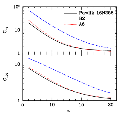
Figure 10.— Here we compare clumping factors $C_{-1}$ and $C_{100}$ from our fiducial simulation B2 ($512^{3}$, 0.5 Mpc) to the Pawlik et al. (2009) simulation L6N256 ($256^{3}$, 6 Mpc). The Pawlik et al. curve corresponds to their reference simulation that did not include photoionization and has similar attributes to our simulation A6 ($256^{3}$, 8 Mpc). As expected, A6 and L6N256 are in good agreement with each other while the higher-resolved simulation B2 shows clumping factors a few times larger than L6N256.

Pawlik et al. (2009) demonstrate convergence of their clumping factor for the heated IGM while noting that convergence would be more difficult to obtain for an unheated IGM. We have explicitly demonstrated this latter point here and accordingly show that their values for the clumping factor are likely underestimates during the initial stages of reionization, by about a factor of a few. This is illustrated in Figure 10 where we compare clumping factors from two of our simulations to the unheated simulation L6N256 of Pawlik et al. Here we plot the clumping factors $C_{-1}$ and $C_{100}$ with this notation being used to emphasize that these clumping factors are evaluated using all gas below some density cutoff. For $C_{-1}$ a physical density threshold of $n_{\rm crit}=0.1~{}{\rm cm}^{-3}$ is used while an overdensity threshold of $\Delta_{\rm crit}=100$ is used for $C_{100}$. These definitions differ from the definition of $c_{l}$ in equation (11) that we have been using so far which involves an average over all ionized gas in the box. In any event, the clumping factors we find in our fiducial simulation B2 are at all times larger, by a factor of 1.2 at $z=20$ and 3.5 at $z=6$ for $C_{-1}$. As described above, the clumping factors we obtain at low redshift are overestimates, and in reality should be closer to $C_{-1}\sim 6$ or $C_{100}\sim 3$ found by Pawlik et al. in the presence of a photoevaporative background. Combining these two results, the clumping factor of the the IGM evolves strongly just after a patch of IGM is ionized. For ionization at $z=9$, the clumping factor drops from $c_{l}\sim 20$ at $z=9$ to a few at $z=6$, depending on the intensity of the ionizing background – with larger intensities leading to higher clumping factors and larger mean free paths. This strong suppression of the clumping factor due to photoheating was demonstrated by Pawlik et al. who referred to it as a positive feedback on reionization since it reduces the total number of recombinations occurring within small-scale absorption systems.

The results presented here for the inhomogeneity of electron density in the presence of an ionizing background should serve as a foundation for more detailed study of radiative transfer and hydrodynamical effects in the initial stages of reionization, including the effects of the initial relative velocity between baryons and dark matter (e.g., Tseliakhovich & Hirata, 2010), preheating by long mean free path X-ray photons (e.g., Ricotti & Ostriker, 2004; Ricotti et al., 2005), and photoevaporation (e.g., Shapiro et al., 2004; Abel et al., 2007). In simulating all of these processes, it will be necessary to resolve small-scale structure in the way outlined here.

References

- Abel et al. (2002) Abel, T., Bryan, G. L., & Norman, M. L. 2002, Science, 295, 93
- Abel et al. (2007) Abel, T., Wise, J. H., & Bryan, G. L. 2007, ApJ, 659, L87
- Alvarez & Abel (2012) Alvarez, M. A. & Abel, T. 2012, ApJ, 747, 126
- Alvarez et al. (2006) Alvarez, M. A., Bromm, V., & Shapiro, P. R. 2006, ApJ, 639, 621
- Alvarez et al. (2012) Alvarez, M. A., Finlator, K., & Trenti, M. 2012, ApJ, 759, L38
- Barkana & Loeb (1999) Barkana, R. & Loeb, A. 1999, ApJ, 523, 54
- Barkana & Loeb (2004) —. 2004, ApJ, 609, 474
- Bolton & Haehnelt (2007) Bolton, J. S. & Haehnelt, M. G. 2007, MNRAS, 382, 325
- Bouwens et al. (2010) Bouwens, R. J., Illingworth, G. D., Oesch, P. A., Stiavelli, M., van Dokkum, P., Trenti, M., Magee, D., Labbé, I., Franx, M., Carollo, C. M., & Gonzalez, V. 2010, ApJ, 709, L133
- Bromm et al. (2002) Bromm, V., Coppi, P. S., & Larson, R. B. 2002, ApJ, 564, 23
- Chiu et al. (2003) Chiu, W. A., Fan, X., & Ostriker, J. P. 2003, ApJ, 599, 759
- Choudhury et al. (2009) Choudhury, T. R., Haehnelt, M. G., & Regan, J. 2009, MNRAS, 394, 960
- Ciardi et al. (2006) Ciardi, B., Scannapieco, E., Stoehr, F., Ferrara, A., Iliev, I. T., & Shapiro, P. R. 2006, MNRAS, 366, 689
- Couchman & Rees (1986) Couchman, H. M. P. & Rees, M. J. 1986, MNRAS, 221, 53
- Fan et al. (2006) Fan, X., Strauss, M. A., Becker, R. H., White, R. L., Gunn, J. E., Knapp, G. R., Richards, G. T., Schneider, D. P., Brinkmann, J., & Fukugita, M. 2006, AJ, 132, 117
- Finlator et al. (2012) Finlator, K., Oh, S. P., Özel, F., & Davé, R. 2012, ArXiv e-prints
- Furlanetto et al. (2004) Furlanetto, S. R., Zaldarriaga, M., & Hernquist, L. 2004, ApJ, 613, 1
- Gnedin & Fan (2006) Gnedin, N. Y. & Fan, X. 2006, ApJ, 648, 1
- Gnedin & Hui (1998) Gnedin, N. Y. & Hui, L. 1998, MNRAS, 296, 44
- Gnedin & Ostriker (1997) Gnedin, N. Y. & Ostriker, J. P. 1997, ApJ, 486, 581
- Greif et al. (2008) Greif, T. H., Johnson, J. L., Klessen, R. S., & Bromm, V. 2008, MNRAS, 387, 1021
- Haardt & Madau (1996) Haardt, F. & Madau, P. 1996, ApJ, 461, 20
- Haiman (2011) Haiman, Z. 2011, Nature, 472, 47
- Haiman et al. (2001) Haiman, Z., Abel, T., & Madau, P. 2001, ApJ, 551, 599
- Haiman et al. (2000) Haiman, Z., Abel, T., & Rees, M. J. 2000, ApJ, 534, 11
- Iliev et al. (2006) Iliev, I. T., Mellema, G., Pen, U.-L., Merz, H., Shapiro, P. R., & Alvarez, M. A. 2006, MNRAS, 369, 1625
- Iliev et al. (2005a) Iliev, I. T., Scannapieco, E., & , P. R. 2005a, ApJ, 624, 491
- Iliev et al. (2005b) Iliev, I. T., Shapiro, P. R., & Raga, A. C. 2005b, MNRAS, 361, 405
- Johnson et al. (2007) Johnson, J. L., Greif, T. H., & Bromm, V. 2007, ApJ, 665, 85
- Komatsu et al. (2011) Komatsu, E., Smith, K. M., Dunkley, J., Bennett, C. L., Gold, B., Hinshaw, G., Jarosik, N., Larson, D., Nolta, M. R., Page, L., Spergel, D. N., Halpern, M., Hill, R. S., Kogut, A., Limon, M., Meyer, S. S., Odegard, N., Tucker, G. S., Weiland, J. L., Wollack, E., & Wright, E. L. 2011, ApJS, 192, 18
- Kuhlen & Faucher-Giguère (2012) Kuhlen, M. & Faucher-Giguère, C.-A. 2012, MNRAS, 423, 862
- Madau et al. (1999) Madau, P., Haardt, F., & Rees, M. J. 1999, ApJ, 514, 648
- McQuinn et al. (2011) McQuinn, M., Oh, S. P., & Faucher-Giguère, C.-A. 2011, ApJ, 743, 82
- Mirabel et al. (2011) Mirabel, I. F., Dijkstra, M., Laurent, P., Loeb, A., & Pritchard, J. R. 2011, A&A, 528, A149
- Miralda-Escudé et al. (2000) Miralda-Escudé, J., Haehnelt, M., & Rees, M. J. 2000, ApJ, 530, 1
- Oesch et al. (2012) Oesch, P. A., Bouwens, R. J., Illingworth, G. D., Labbé, I., Trenti, M., Gonzalez, V., Carollo, C. M., Franx, M., van Dokkum, P. G., & Magee, D. 2012, ApJ, 745, 110
- Oh & Haiman (2003) Oh, S. P. & Haiman, Z. 2003, MNRAS, 346, 456
- Pawlik et al. (2009) Pawlik, A. H., Schaye, J., & van Scherpenzeel, E. 2009, MNRAS, 394, 1812
- Peebles & Dicke (1968) Peebles, P. J. E. & Dicke, R. H. 1968, ApJ, 154, 891
- Prochaska et al. (2009) Prochaska, J. X., O’Meara, J. M., & Worseck, G. 2009, arXiv:0912.0292
- Reed et al. (2007) Reed, D. S., Bower, R., Frenk, C. S., Jenkins, A., & Theuns, T. 2007, MNRAS, 374, 2
- Ricotti & Ostriker (2004) Ricotti, M. & Ostriker, J. P. 2004, MNRAS, 352, 547
- Ricotti et al. (2005) Ricotti, M., Ostriker, J. P., & Gnedin, N. Y. 2005, MNRAS, 357, 207
- Shapiro & Giroux (1987) Shapiro, P. R. & Giroux, M. L. 1987, ApJ, 321, L107
- Shapiro et al. (1994) Shapiro, P. R., Giroux, M. L., & Babul, A. 1994, ApJ, 427, 25
- Shapiro et al. (2004) Shapiro, P. R., Iliev, I. T., & Raga, A. C. 2004, MNRAS, 348, 753
- Shull et al. (2012) Shull, J. M., Harness, A., Trenti, M., & Smith, B. D. 2012, ApJ, 747, 100
- Springel (2005) Springel, V. 2005, MNRAS, 364, 1105
- Storrie-Lombardi et al. (1994) Storrie-Lombardi, L. J., McMahon, R. G., Irwin, M. J., & Hazard, C. 1994, ApJ, 427, L13
- Tegmark et al. (1997) Tegmark, M., Silk, J., Rees, M. J., Blanchard, A., Abel, T., & Palla, F. 1997, ApJ, 474, 1
- Trenti et al. (2010) Trenti, M., Stiavelli, M., Bouwens, R. J., Oesch, P., Shull, J. M., Illingworth, G. D., Bradley, L. D., & Carollo, C. M. 2010, ApJ, 714, L202
- Tseliakhovich & Hirata (2010) Tseliakhovich, D. & Hirata, C. 2010, Phys. Rev. D, 82, 083520
- Warren et al. (2006) Warren, M. S., Abazajian, K., Holz, D. E., & Teodoro, L. 2006, ApJ, 646, 881
- Wise & Abel (2008) Wise, J. H. & Abel, T. 2008, ApJ, 685, 40
- Wise & Cen (2009) Wise, J. H. & Cen, R. 2009, ApJ, 693, 984
- Wise et al. (2012) Wise, J. H., Turk, M. J., Norman, M. L., & Abel, T. 2012, ApJ, 745, 50
- Yoshida et al. (2003) Yoshida, N., Abel, T., Hernquist, L., & Sugiyama, N. 2003, ApJ, 592, 645
- Yoshida et al. (2007) Yoshida, N., Oh, S. P., Kitayama, T., & Hernquist, L. 2007, ApJ, 663, 687