Scattering function of semiflexible polymer chains under good solvent conditions

Hsiao-Ping Hsua, Wolfgang Paulb, and Kurt Bindera aInstitut fΓΌr Physik, Johannes Gutenberg-UniversitΓ€t Mainz,
Staudinger Weg 7, D-55099 Mainz, Germany
bTheoretische Physik, Martin Luther UniversitΓ€t
Halle-Wittenberg, von Seckendorffplatz 1, 06120 Halle, Germany
Abstract

Using the pruned-enriched Rosenbluth Monte Carlo algorithm, the scattering functions of semiflexible macromolecules in dilute solution under good solvent conditions are estimated both in d=2𝑑2d=2 and d=3𝑑3d=3 dimensions, considering also the effect of stretching forces. Using self-avoiding walks of up to N=25600𝑁25600N=25600 steps on the square and simple cubic lattices, variable chain stiffness is modeled by introducing an energy penalty Ο΅bsubscriptitalic-ϡ𝑏\epsilon_{b} for chain bending; varying qb=exp⁑(βˆ’Ο΅b/kB​T)subscriptπ‘žπ‘subscriptitalic-ϡ𝑏subscriptπ‘˜π΅π‘‡q_{b}=\exp(-\epsilon_{b}/k_{B}T) from qb=1subscriptπ‘žπ‘1q_{b}=1 (completely flexible chains) to qb=0.005subscriptπ‘žπ‘0.005q_{b}=0.005, the persistence length can be varied over two orders of magnitude. For unstretched semiflexible chains we test the applicability of the Kratky-Porod worm-like chain model to describe the scattering function, and discuss methods for extracting persistence length estimates from scattering. While in d=2𝑑2d=2 the direct crossover from rod-like chains to self-avoiding walks invalidates the Kratky-Porod description, it holds in d=3𝑑3d=3 for stiff chains if the number of Kuhn segments nKsubscript𝑛𝐾n_{K} does not exceed a limiting value nKβˆ—subscriptsuperscript𝑛𝐾n^{*}_{K} (which depends on the persistence length). For stretched chains, the Pincus blob size enters as a further characteristic length scale. The anisotropy of the scattering is well described by the modified Debye function, if the actual observed chain extension ⟨X⟩delimited-βŸ¨βŸ©π‘‹\langle X\rangle (end-to-end distance in the direction of the force) as well as the corresponding longitudinal and transverse linear dimensions ⟨X2βŸ©βˆ’βŸ¨X⟩2delimited-⟨⟩superscript𝑋2superscriptdelimited-βŸ¨βŸ©π‘‹2\langle X^{2}\rangle-\langle X\rangle^{2}, ⟨Rg,βŠ₯2⟩delimited-⟨⟩superscriptsubscript𝑅𝑔bottom2\langle R_{g,\bot}^{2}\rangle are used.

I Introduction

Small angle (neutron) scattering from polymers in dilute solution is the method of choice to obtain a complete picture of the conformations of long flexible or semiflexible macromolecules, from the length scale of the monomeric units to the gyration radius of the chain moleculesΒ 1 ; 2 ; 3 ; 4 . Classical experiments have shown that the gyration radius Rgsubscript𝑅𝑔R_{g} of long flexible chains in dense melts (and also in dilute solution under Theta conditions) scales with chain length N according to the classical random walk pictureΒ 5 ; 6 ; 7 , Rg∝N1/2proportional-tosubscript𝑅𝑔superscript𝑁12R_{g}\propto N^{1/2}, while in dilute solution under good solvent conditions flexible polymers form swollen coilsΒ 1 ; 2 ; 3 ; 4 ; 8 , Rg∝NΞ½proportional-tosubscript𝑅𝑔superscriptπ‘πœˆR_{g}\propto N^{\nu}, withΒ 9 Ξ½β‰ˆ0.588𝜈0.588\nu\approx 0.588 (in d=3𝑑3d=3 dimensions) or Ξ½=3/4​(d=2)𝜈34𝑑2\nu=3/4\;(d=2). It was also shown that on intermediate length scales the dependence of the scattering intensity S​(q)π‘†π‘žS(q) on wave number qπ‘žq reflects the self-similar fractal structure of the polymerΒ 8 , S​(q)∝qβˆ’1/Ξ½proportional-toπ‘†π‘žsuperscriptπ‘ž1𝜈S(q)\propto q^{-1/\nu} (under good solvent conditions) or S​(q)∝qβˆ’2proportional-toπ‘†π‘žsuperscriptπ‘ž2S(q)\propto q^{-2} (Theta conditions or melts, respectively). Also the crossovers between these regimes when either the temperature distance from the Theta point or the concentration of the solution are varied have been investigatedΒ 4 , and the length scales ruling these crossovers (i.e., diameter of β€œthermal blobs” or β€œconcentration blobs”, respectively) have been identifiedΒ 1 ; 2 ; 3 ; 4 .

The behavior gets more complicated, however, when chain stiffness plays a prominent role: only when chain stiffness is essentially due to chain thickness, i.e. when the effective persistence length β„“psubscriptℓ𝑝\ell_{p} scales proportional to the local chain diameter D𝐷D the problem can still be reduced to a rescaled self-avoiding walk problemΒ 10 ; 11 . However, when β„“p≫Dmuch-greater-thansubscriptℓ𝑝𝐷\ell_{p}\gg D, one finds (in d=3𝑑3d=3) a double crossover, since then short chains behave like rigid rods (i.e., Rg∝Nproportional-tosubscript𝑅𝑔𝑁R_{g}\propto N as long as Rg<β„“psubscript𝑅𝑔subscriptℓ𝑝R_{g}<\ell_{p}), and then a crossover to Gaussian random-walk like coils occurs, while for Rgβ‰ˆR0subscript𝑅𝑔subscript𝑅0R_{g}\approx R_{0} (R0subscript𝑅0R_{0} will be discussed below) a second crossover to swollen coils (Rg∝NΞ½)proportional-tosubscript𝑅𝑔superscriptπ‘πœˆ(R_{g}\propto N^{\nu}) starts. Also this behavior has been established in beautiful classical experimentsΒ 12 , as well as in recent simulationsΒ 11 ; 13 . The standard model for semiflexible worm-like chains, the Kratky-Porod modelΒ 14 , can only describe the first crossover (from rods to Gaussian coils) but fails to account for the second crossover to swollen coils, due to its complete neglect of excluded volume effects. It turns out that this second crossover still is incompletely understood: while in the early experimentsΒ 12 it was suggested that this crossover occurs for nK=nKβˆ—subscript𝑛𝐾superscriptsubscript𝑛𝐾n_{K}=n_{K}^{*} with nKβˆ—=50superscriptsubscript𝑛𝐾50n_{K}^{*}=50 Kuhn segments, independent of the persistence length, a Flory-type argumentΒ 15 ; 16 suggests that the crossover occurs for a polymer radius R0βˆβ„“p2/Dproportional-tosubscript𝑅0superscriptsubscriptℓ𝑝2𝐷R_{0}\propto\ell_{p}^{2}/D (corresponding to nKβˆ—βˆ(β„“p/D)2)n^{*}_{K}\propto(\ell_{p}/D)^{2}), while the simulations rather findΒ 13 nKβˆ—βˆβ„“p1.5proportional-tosubscriptsuperscript𝑛𝐾superscriptsubscriptℓ𝑝1.5n^{*}_{K}\propto\ell_{p}^{1.5}. Remember that a worm-like chain can be described as an equivalent freely jointed chain of nksubscriptπ‘›π‘˜n_{k} Kuhn segments of length 2​ℓp2subscriptℓ𝑝2\ell_{p} eachΒ 5 ; 6 . In view of an apparent conflict of the estimateΒ 12 nKβˆ—=50subscriptsuperscript𝑛𝐾50n^{*}_{K}=50 with the Yamakawa-Stockmayer-Shimata theoryΒ 16 ; 161 ; 162 ; 163 for worm-like chains the result nKβˆ—=50subscriptsuperscript𝑛𝐾50n^{*}_{K}=50 was considered as a very fundamental problemΒ 164 ; 165 . However, Tsuboi et alΒ 165 confirmed this estimate for another stiff polymer and concluded that the result nKβˆ—=50subscriptsuperscript𝑛𝐾50n^{*}_{K}=50 is compatible with the theory. We also note that in d=2𝑑2d=2 there occurs a single crossover from rods to self-avoiding walks, any regime of Gaussian-like behavior is completely absentΒ 13 ; 17 . We emphasize however, that the results ofΒ 11 ; 13 ; 15 ; 16 imply that a universal number nKβˆ—superscriptsubscript𝑛𝐾n_{K}^{*} (independent of β„“psubscriptℓ𝑝\ell_{p}) up to which the Kratky-Porod model holds in d=3𝑑3d=3 does not exist.

It then is interesting to ask how chain stiffness shows up on intermediate length scales, that can be probed via the scattering function S​(q)π‘†π‘žS(q). If one disregards excluded volumeΒ 1 and bases the treatment on the Kratky-Porod model, one can showΒ 18 that the rod-like behavior at large qπ‘žq leads to a scattering law proportional to qβˆ’1superscriptπ‘ž1q^{-1}, i.e. (in d=3𝑑3d=3 dimensions)

N​ℓb​q​S​(q)=Ο€+23​(q​ℓp)βˆ’1,Nβ†’βˆž,formulae-sequence𝑁subscriptβ„“π‘π‘žπ‘†π‘žπœ‹23superscriptπ‘žsubscriptℓ𝑝1→𝑁N\ell_{b}qS(q)=\pi+\frac{2}{3}(q\ell_{p})^{-1}\,,\qquad N\rightarrow\infty\,, (1)

where we have assumed that the chain has a contour length L=N​ℓb𝐿𝑁subscriptℓ𝑏L=N\ell_{b}, where β„“bsubscriptℓ𝑏\ell_{b} is the bond length while the persistence lengthΒ 6 is β„“p=(N/nK)​ℓb/2subscriptℓ𝑝𝑁subscript𝑛𝐾subscriptℓ𝑏2\ell_{p}=(N/n_{K})\ell_{b}/2. While for Gaussian β€œphantom chains” (i.e., excluded volume interactions are completely neglected) the structure factor S​(q)π‘†π‘žS(q) is readily foundΒ 1 ; 2 ; 3 ; 4 ; 5 ; 6 in terms of the Debye function, and the only length that enters is the gyration radius ⟨Rg2⟩1/2superscriptdelimited-⟨⟩superscriptsubscript𝑅𝑔212\langle R_{g}^{2}\rangle^{1/2}, choosing a normalization where S​(q=0)=1π‘†π‘ž01S(q=0)=1

S​(q)=2​[exp⁑(βˆ’ΞΆ)βˆ’1+ΞΆ]/ΞΆ2,ΞΆ=q2β€‹βŸ¨Rg2⟩=q2​N​ℓb2/6,formulae-sequenceπ‘†π‘ž2delimited-[]𝜁1𝜁superscript𝜁2𝜁superscriptπ‘ž2delimited-⟨⟩superscriptsubscript𝑅𝑔2superscriptπ‘ž2𝑁superscriptsubscriptℓ𝑏26S(q)=2[\exp(-\zeta)-1+\zeta]/\zeta^{2}\,,\,\zeta=q^{2}\langle R_{g}^{2}\rangle=q^{2}N\ell_{b}^{2}/6\,, (2)

for semiflexible polymers the calculation of S​(q)π‘†π‘žS(q) for chains with N𝑁N finite is a formidable problemΒ 19 ; 20 ; 21 ; 22 ; 23 ; 231 ; 24 ; 25 ; 26 ; 27 ; 271 ; 28 ; 281 ; 29 ; 291 ; 292 , even in the absence of excluded volume effects. However, including excluded volume effects in the description of scattering of semiflexible chains is even more an unsolved problem: existing phenomenological approaches require the adjustment of many empirical parametersΒ 29 . It will be one of the tasks that will be addressed in the present paper, to investigate S​(q)π‘†π‘žS(q) for semiflexible chains numerically in the presence of excluded volume interactions between the effective monomers, varying β„“psubscriptℓ𝑝\ell_{p} over a wide range.

In recent years also the behavior of macromolecules under the influence of stretching forces has found enormous interest (e.g.Β 30 ; 31 ; 32 ; 33 ; 34 ; 35 ; 36 ; 37 ; 38 ; 39 ; 40 ; 41 ; 42 ; 43 ; 44 ; 45 ), in particular for the study of bio-macromolecules. Experimentally this can be realized e.g. by pulling at one end of a chain, that is anchored at a substrate with the other chain end, by the tip of an atomic force microscopeΒ 32 ; 36 ; 38 ; 39 ; 42 ; 45 but it is also conceivable to stretch polymers by the forces occurring when a polymer solution is exposed to strong shear flowΒ 46 ; 461 ; 462 or elongational flowΒ 463 . Of course, it is not obvious that it will be possible to carry out scattering experiments on such stretched chains and measure the structure factor (which then is anisotropic and has two relevant parts S||​(q||)S_{||}(q_{||}), SβŠ₯​(qβŠ₯)subscript𝑆bottomsubscriptπ‘žbottomS_{\bot}(q_{\bot}) since the direction of the scattering vector qβ†’β†’π‘ž\vec{q} relative to the stretch direction, either parallel, q||q_{||}, or perpendicular, qβŠ₯subscriptπ‘žbottomq_{\bot}, matters). But nevertheless a theoretical investigation of S||​(q||),SβŠ₯​(qβŠ₯)S_{||}(q_{||}),S_{\bot}(q_{\bot}) is worthwhile, because it gives detailed insight into the local structure of stretched chains, including also chains under cylindrical confinementΒ 47 ; 48 ; 49 and this may help to understand problems such as transport of semiflexible polymers through porous materials, or channels in nanofluidic devicesΒ 47 , etc. Thus we shall also investigate the structure factor of stretched semiflexible chains, extending previous work on flexible chainsΒ 30 ; 34 .

The outline of our paper is as follows: in Sec. II, we give a summary of the theoretical background, and in Sec. III we define our model and briefly recall the simulation methodology. In Sec. IV we present our results for the structure factor S​(q)π‘†π‘žS(q) of semiflexible chains, for both d=2𝑑2d=2 and d=3𝑑3d=3 dimensions, in the absence of stretching forces. Sec. V describes the modifications of the structure factor due to stretching, while Sec. VI summarizes our conclusions. The calculation of the scattering function of random walk chains under constant pulling forces can be carried out analytically and is presented in an appendix.

II Theoretical Background

II.1 Definitions

We consider here the scattering from a single polymer chain, assuming that the chain can be described by a sequence of N+1𝑁1N+1 (effective) monomers at positions rβ†’jsubscriptβ†’π‘Ÿπ‘—\vec{r}_{j}, j=1,2,…𝑗12…j=1,2,\ldots, N+1𝑁1N+1, so that we can define N𝑁N bond vectors aβ†’j=rβ†’j+1βˆ’rβ†’jsubscriptβ†’π‘Žπ‘—subscriptβ†’π‘Ÿπ‘—1subscriptβ†’π‘Ÿπ‘—\vec{a}_{j}=\vec{r}_{j+1}-\vec{r}_{j}. In the absence of stretching forces, the structure factor S​(qβ†’)π‘†β†’π‘žS(\vec{q}) does not depend on the direction of the scattering vector qβ†’β†’π‘ž\vec{q}, and can be defined as

S​(q)π‘†π‘ž\displaystyle S(q) =\displaystyle= 1(N+1)2β€‹βŸ¨βˆ‘j=1N+1βˆ‘k=1N+1exp⁑[i​qβ†’β‹…(rβ†’jβˆ’rβ†’k)]⟩1superscript𝑁12delimited-⟨⟩superscriptsubscript𝑗1𝑁1superscriptsubscriptπ‘˜1𝑁1β‹…π‘–β†’π‘žsubscriptβ†’π‘Ÿπ‘—subscriptβ†’π‘Ÿπ‘˜\displaystyle\frac{1}{(N+1)^{2}}\left\langle\sum\limits_{j=1}^{N+1}\;\sum\limits_{k=1}^{N+1}\exp[i\vec{q}\cdot(\vec{r}_{j}-\vec{r}_{k})]\right\rangle (3)
=\displaystyle= 1(N+1)2​{⟨[βˆ‘j=1N+1sin⁑(qβ†’β‹…rβ†’j)]2⟩+⟨[βˆ‘j=1N+1cos⁑(qβ†’β‹…rβ†’j)]2⟩}.1superscript𝑁12delimited-⟨⟩superscriptdelimited-[]superscriptsubscript𝑗1𝑁1β‹…β†’π‘žsubscriptβ†’π‘Ÿπ‘—2delimited-⟨⟩superscriptdelimited-[]superscriptsubscript𝑗1𝑁1β‹…β†’π‘žsubscriptβ†’π‘Ÿπ‘—2\displaystyle\frac{1}{(N+1)^{2}}\left\{\left\langle\left[\sum\limits_{j=1}^{N+1}\sin(\vec{q}\cdot\vec{r}_{j})\right]^{2}\right\rangle+\left\langle\left[\sum\limits_{j=1}^{N+1}\cos(\vec{q}\cdot\vec{r}_{j})\right]^{2}\right\rangle\right\}\,.

Note that we have chosen here a normalization for which S​(qβ†’0)=1π‘†β†’π‘ž01S(q\rightarrow 0)=1. When a stretching force is applied to one chain end in the +x-direction, the structure factor becomes anisotropic. In d=3𝑑3d=3 dimensions, the conformations of chains still have axis-symmetric geometries, and we must distinguish between S||​(q||)S_{||}(q_{||}), where qβ†’β†’π‘ž\vec{q} is oriented in the x-direction parallel to the force, and SβŠ₯​(qβ†’βŠ₯)subscript𝑆bottomsubscriptβ†’π‘žbottomS_{\bot}(\vec{q}_{\bot}), where qβ†’β†’π‘ž\vec{q} is oriented perpendicular to it. So we define rβ†’j=(xj,yj,zj)=(xj,ρ→j)subscriptβ†’π‘Ÿπ‘—subscriptπ‘₯𝑗subscript𝑦𝑗subscript𝑧𝑗subscriptπ‘₯𝑗subscriptβ†’πœŒπ‘—\vec{r}_{j}=(x_{j},y_{j},z_{j})=(x_{j},\vec{\rho}_{j}) to obtain

S||​(q||)=1(N+1)2​{⟨[βˆ‘j=1N+1sin⁑(q||​xj)]2⟩+⟨[βˆ‘j=1N+1cos⁑(q||​xj)]2⟩},S_{||}(q_{||})=\frac{1}{(N+1)^{2}}\left\{\left\langle\left[\sum\limits_{j=1}^{N+1}\sin(q_{||}x_{j})\right]^{2}\right\rangle+\left\langle\left[\sum\limits_{j=1}^{N+1}\cos(q_{||}x_{j})\right]^{2}\right\rangle\right\}\,, (4)
SβŠ₯​(qβŠ₯)=1(N+1)2​{⟨[βˆ‘j=1N+1sin⁑(qβ†’βŠ₯⋅ρ→j)]2⟩+⟨[βˆ‘j=1N+1cos⁑(qβ†’βŠ₯⋅ρ→j)]2⟩}.subscript𝑆bottomsubscriptπ‘žbottom1superscript𝑁12delimited-⟨⟩superscriptdelimited-[]superscriptsubscript𝑗1𝑁1β‹…subscriptβ†’π‘žbottomsubscriptβ†’πœŒπ‘—2delimited-⟨⟩superscriptdelimited-[]superscriptsubscript𝑗1𝑁1β‹…subscriptβ†’π‘žbottomsubscriptβ†’πœŒπ‘—2S_{\bot}(q_{\bot})=\frac{1}{(N+1)^{2}}\left\{\left\langle\left[\sum\limits_{j=1}^{N+1}\sin(\vec{q}_{\bot}\cdot\vec{\rho}_{j})\right]^{2}\right\rangle+\left\langle\left[\sum\limits_{j=1}^{N+1}\cos(\vec{q}_{\bot}\cdot\vec{\rho}_{j})\right]^{2}\right\rangle\right\}\,. (5)

Note that in d=2𝑑2d=2 dimensions we have rβ†’j=(xj,yj)subscriptβ†’π‘Ÿπ‘—subscriptπ‘₯𝑗subscript𝑦𝑗\vec{r}_{j}=(x_{j},y_{j}) and then qβ†’βŠ₯⋅ρ→jβ‹…subscriptβ†’π‘žbottomsubscriptβ†’πœŒπ‘—\vec{q}_{\bot}\cdot\vec{\rho}_{j} in Eq.Β (5) needs to be replaced simply by qβŠ₯​yjsubscriptπ‘žbottomsubscript𝑦𝑗q_{\bot}y_{j}, of course.

We also stress that in this paper we are not at all concerned with effects due to the local structure of (effective) monomers, such as e.g. chemical side groups, etc.; such effects show up at large qπ‘žq when one considers the scattering from real chainsΒ 231 . We next define our notation for characteristic lengths of the chain. Assuming a rigidly fixed bond length β„“bsubscriptℓ𝑏\ell_{b} between neighboring monomers along the chain, the contour length L𝐿L is

L=N​ℓb𝐿𝑁subscriptℓ𝑏L=N\ell_{b} (6)

The mean square end-to-end distance (in the absence of stretching forces) simply is

⟨R2⟩=⟨(βˆ‘j=1Naβ†’j)2⟩delimited-⟨⟩superscript𝑅2delimited-⟨⟩superscriptsuperscriptsubscript𝑗1𝑁subscriptβ†’π‘Žπ‘—2\langle R^{2}\rangle=\left\langle\left(\sum\limits_{j=1}^{N}\vec{a}_{j}\right)^{2}\right\rangle (7)

with aβ†’j=rβ†’j+1βˆ’rβ†’jsubscriptβ†’π‘Žπ‘—subscriptβ†’π‘Ÿπ‘—1subscriptβ†’π‘Ÿπ‘—\vec{a}_{j}=\vec{r}_{j+1}-\vec{r}_{j} being the j-th bond vector, and the mean square gyration radius is given by

⟨Rg2⟩delimited-⟨⟩superscriptsubscript𝑅𝑔2\displaystyle\langle R_{g}^{2}\rangle =\displaystyle= 1N+1β€‹βŸ¨βˆ‘j=1N+1(rβ†’jβˆ’rβ†’C​M)2⟩1𝑁1delimited-⟨⟩superscriptsubscript𝑗1𝑁1superscriptsubscriptβ†’π‘Ÿπ‘—subscriptβ†’π‘ŸπΆπ‘€2\displaystyle\frac{1}{N+1}\left\langle\sum\limits_{j=1}^{N+1}(\vec{r}_{j}-\vec{r}_{CM})^{2}\right\rangle (8)
=\displaystyle= 1(N+1)2β€‹βŸ¨βˆ‘j=1N+1βˆ‘k=j+1N+1(rβ†’jβˆ’rβ†’k)2⟩,1superscript𝑁12delimited-⟨⟩superscriptsubscript𝑗1𝑁1superscriptsubscriptπ‘˜π‘—1𝑁1superscriptsubscriptβ†’π‘Ÿπ‘—subscriptβ†’π‘Ÿπ‘˜2\displaystyle\frac{1}{(N+1)^{2}}\left\langle\sum\limits_{j=1}^{N+1}\sum\limits_{k=j+1}^{N+1}(\vec{r}_{j}-\vec{r}_{k})^{2}\right\rangle\,,

where rβ†’C​M=βˆ‘j=1N+1rβ†’j/(N+1)subscriptβ†’π‘ŸπΆπ‘€superscriptsubscript𝑗1𝑁1subscriptβ†’π‘Ÿπ‘—π‘1\vec{r}_{CM}=\sum\limits_{j=1}^{N+1}\vec{r}_{j}/(N+1) is the center of mass position of the polymer.

In the presence of stretching forces, the chain takes a mean extension ⟨X⟩delimited-βŸ¨βŸ©π‘‹\langle X\rangle and mean square extensions also become anisotropic,

⟨X⟩=βŸ¨βˆ‘j=1Naj​x⟩,⟨X2⟩=⟨(βˆ‘j=1Naj​x)2⟩,formulae-sequencedelimited-βŸ¨βŸ©π‘‹delimited-⟨⟩superscriptsubscript𝑗1𝑁subscriptπ‘Žπ‘—π‘₯delimited-⟨⟩superscript𝑋2delimited-⟨⟩superscriptsubscriptsuperscript𝑁𝑗1subscriptπ‘Žπ‘—π‘₯2\langle X\rangle=\left\langle\sum\limits_{j=1}^{N}a_{jx}\right\rangle\,,\qquad\left\langle X^{2}\right\rangle=\left\langle\left(\sum\limits^{N}_{j=1}a_{jx}\right)^{2}\right\rangle\,, (9)
⟨RβŠ₯2⟩=⟨(βˆ‘j=1Naj​y)2⟩+⟨(βˆ‘j=1Naj​z)2⟩.delimited-⟨⟩subscriptsuperscript𝑅2bottomdelimited-⟨⟩superscriptsuperscriptsubscript𝑗1𝑁subscriptπ‘Žπ‘—π‘¦2delimited-⟨⟩superscriptsuperscriptsubscript𝑗1𝑁subscriptπ‘Žπ‘—π‘§2\langle R^{2}_{\bot}\rangle=\left\langle\left(\sum\limits_{j=1}^{N}a_{jy}\right)^{2}\right\rangle+\left\langle\left(\sum\limits_{j=1}^{N}a_{jz}\right)^{2}\right\rangle\;. (10)

Eq.Β (10) refers to the three-dimensional case, for d=2𝑑2d=2 the second term in the right hand side needs to be omitted. A related anisotropy can then be stated for the gyration radius square as well, namely

⟨Rg,||2⟩=1(N+1)2β€‹βŸ¨βˆ‘j=1N+1βˆ‘k=j+1N+1(xjβˆ’xk)2⟩,\langle R_{g,||}^{2}\rangle=\frac{1}{(N+1)^{2}}\left\langle\sum\limits_{j=1}^{N+1}\sum\limits_{k=j+1}^{N+1}(x_{j}-x_{k})^{2}\right\rangle\,, (11)
⟨Rg,βŠ₯2⟩=1(N+1)2β€‹βŸ¨βˆ‘j=1N+1βˆ‘k=j+1N+1[(yjβˆ’yk)2+(zjβˆ’zk)2]⟩,delimited-⟨⟩superscriptsubscript𝑅𝑔bottom21superscript𝑁12delimited-⟨⟩superscriptsubscript𝑗1𝑁1superscriptsubscriptπ‘˜π‘—1𝑁1delimited-[]superscriptsubscript𝑦𝑗subscriptπ‘¦π‘˜2superscriptsubscript𝑧𝑗subscriptπ‘§π‘˜2\langle R_{g,\bot}^{2}\rangle=\frac{1}{(N+1)^{2}}\left\langle\sum\limits_{j=1}^{N+1}\sum\limits_{k=j+1}^{N+1}\left[(y_{j}-y_{k})^{2}+(z_{j}-z_{k})^{2}\right]\right\rangle\,, (12)

for d=3𝑑3d=3, again the term (zjβˆ’zk)2superscriptsubscript𝑧𝑗subscriptπ‘§π‘˜2(z_{j}-z_{k})^{2} simply is omitted in the case d=2𝑑2d=2.

We also recall that the mean square gyration radii describe the scattering functions at small qβ†’β†’π‘ž\vec{q}. So in the absence of stretching forces we have

S​(q)=1βˆ’q2β€‹βŸ¨Rg2⟩/d,qβ†’0,formulae-sequenceπ‘†π‘ž1superscriptπ‘ž2delimited-⟨⟩superscriptsubscript𝑅𝑔2π‘‘β†’π‘ž0S(q)=1-q^{2}\langle R_{g}^{2}\rangle/d\,,\qquad q\rightarrow 0\,, (13)

while if stretching forces are present, one finds instead

S||​(q||)=1βˆ’q||2β€‹βŸ¨Rg,||2⟩,qβ†’0,S_{||}(q_{||})=1-q^{2}_{||}\langle R_{g,||}^{2}\rangle\,,\qquad q\rightarrow 0\,, (14)
SβŠ₯​(qβŠ₯)=1βˆ’qβŠ₯2β€‹βŸ¨Rg,βŠ₯2⟩/(dβˆ’1),qβ†’0.formulae-sequencesubscript𝑆bottomsubscriptπ‘žbottom1superscriptsubscriptπ‘žbottom2delimited-⟨⟩superscriptsubscript𝑅𝑔bottom2𝑑1β†’π‘ž0S_{\bot}(q_{\bot})=1-q_{\bot}^{2}\langle R_{g,\bot}^{2}\rangle/(d-1)\,,\qquad q\rightarrow 0\,. (15)

In addition to the limit qβ†’0β†’π‘ž0q\rightarrow 0, also the limiting behavior of S​(qβ†’βˆž)π‘†β†’π‘žS(q\rightarrow\infty) is trivially known: then all interference terms in Eq.Β (3) average to zero, and only the terms j=kπ‘—π‘˜j=k contribute to the double sum. Hence we obtain

S​(qβ†’βˆž)π‘†β†’π‘ž\displaystyle S(q\rightarrow\infty) =\displaystyle= 1N+1,1𝑁1\displaystyle\frac{1}{N+1}\,,
S||​(q||β†’βˆž)\displaystyle S_{||}(q_{||}\rightarrow\infty) =\displaystyle= SβŠ₯​(qβŠ₯β†’βˆž)=1N+1,subscript𝑆bottomβ†’subscriptπ‘žbottom1𝑁1\displaystyle S_{\bot}(q_{\bot}\rightarrow\infty)=\frac{1}{N+1}\,, (16)

irrespective of the value of the persistence length β„“psubscriptℓ𝑝\ell_{p}, the value of an applied force f𝑓f, etc.

At this point we emphasize, however, that it is not possible to write down a general definition for the persistence length β„“psubscriptℓ𝑝\ell_{p} that would be both universally valid and practically usefulΒ 10 ; 11 ; 13 . The definition often found in textbooksΒ 6 ; 50 in terms of the asymptotic decay of the bond vector orientational function (of a very long chain, Nβ†’βˆž)N\rightarrow\infty)

⟨cos⁑θ​(s)βŸ©β‰‘βŸ¨aβ†’jβ‹…aβ†’j+s⟩/⟨aβ†’jβ‹…aβ†’j⟩∝exp⁑(βˆ’s​ℓb/β„“p),sβ†’βˆžformulae-sequencedelimited-βŸ¨βŸ©πœƒπ‘ delimited-βŸ¨βŸ©β‹…subscriptβ†’π‘Žπ‘—subscriptβ†’π‘Žπ‘—π‘ delimited-βŸ¨βŸ©β‹…subscriptβ†’π‘Žπ‘—subscriptβ†’π‘Žπ‘—proportional-to𝑠subscriptℓ𝑏subscriptℓ𝑝→𝑠\langle\cos\theta(s)\rangle\equiv\langle\vec{a}_{j}\cdot\vec{a}_{j+s}\rangle/\langle\vec{a}_{j}\cdot\vec{a}_{j}\rangle\propto\exp(-s\ell_{b}/\ell_{p})\,,\,s\rightarrow\infty (17)

makes sense only for Gaussian PHANTOM chains, and is not applicable to real polymers under ANY CIRCUMSTANCES, since the asymptotic decay of ⟨cos⁑θ​(s)⟩delimited-βŸ¨βŸ©πœƒπ‘ \langle\cos\theta(s)\rangle with the β€œchemical distance” s​ℓb𝑠subscriptℓ𝑏s\ell_{b} along the chain always is a power-law decay. In fact, for β„“pβ‰ͺs​ℓbβ‰ͺLmuch-less-thansubscriptℓ𝑝𝑠subscriptℓ𝑏much-less-than𝐿\ell_{p}\ll s\ell_{b}\ll L one hasΒ 10 ; 11 ; 13 ; 51 ; 52 ; 53 ; 54

⟨cos⁑θ​(s)⟩∝sβˆ’Ξ²proportional-todelimited-βŸ¨βŸ©πœƒπ‘ superscript𝑠𝛽\langle\cos\theta(s)\rangle\propto s^{-\beta} (18)

where Ξ²=3/2𝛽32\beta=3/2 both in meltsΒ 51 ; 52 and for chains in dilute solution under Theta conditionsΒ 10 ; 53 . For the case of good solvent conditions, which is the problem of interest for the present paper, one rather finds the scaling lawΒ 10 ; 54

Ξ²=2​(1βˆ’Ξ½)𝛽21𝜈\beta=2(1-\nu) (19)

which yields Ξ²=0.825​(d=3)𝛽0.825𝑑3\beta=0.825\;(d=3) and Ξ²=1/2​(d=2)𝛽12𝑑2\beta=1/2\;(d=2), respectively. In simple cases, such as the semiflexible extension of the self-avoiding walk model studied inΒ 13 and further investigated in the present work, one can rather use an analog of Eq.Β (17) but for short chemical distances,

⟨cos⁑θ​(s)⟩=exp⁑(βˆ’s​ℓb/β„“p),0≀s≀ℓp/β„“bformulae-sequencedelimited-βŸ¨βŸ©πœƒπ‘ π‘ subscriptℓ𝑏subscriptℓ𝑝0𝑠subscriptℓ𝑝subscriptℓ𝑏\langle\cos\theta(s)\rangle=\exp(-s\ell_{b}/\ell_{p})\,,\qquad 0\leq s\leq\ell_{p}/\ell_{b} (20)

Eq.Β (20) is useful for the simple model that will be studied in the present paper, namely the self-avoiding walk (SAW) on square and simple cubic lattices with an energy penalty Ο΅bsubscriptitalic-ϡ𝑏\epsilon_{b} for β€œbond bending” (i.e., kinks of the SAW by 90 degrees), which then serves as a convenient parameter to control the persistence length. Since for Ο΅b/kB​T<2subscriptitalic-ϡ𝑏subscriptπ‘˜π΅π‘‡2\epsilon_{b}/k_{B}T<2 the power law, Eq.Β (18), already starts to set in even for small s𝑠s of order unity already, we use in practice an alternative definition,

β„“p/β„“b=βˆ’1/ln⁑(⟨cos⁑θ​(1)⟩),subscriptℓ𝑝subscriptℓ𝑏1delimited-βŸ¨βŸ©πœƒ1\ell_{p}/\ell_{b}=-1/\ln(\langle\cos\theta(1)\rangle)\,, (21)

which is equivalent to Eq.Β (20), if Eq.Β (20) holds over a more extended range of s𝑠s. An alternative method considers the distribution function P​(ns​t​r)𝑃subscriptπ‘›π‘ π‘‘π‘ŸP(n_{str}) of ns​t​rsubscriptπ‘›π‘ π‘‘π‘Ÿn_{str} successive bond vectors aβ†’isubscriptβ†’π‘Žπ‘–\vec{a}_{i} having the same orientation without any kink, which is found to behave asΒ 13 P​(ns​t​r)=ap​exp⁑(βˆ’ns​t​r/np)𝑃subscriptπ‘›π‘ π‘‘π‘Ÿsubscriptπ‘Žπ‘subscriptπ‘›π‘ π‘‘π‘Ÿsubscript𝑛𝑝P(n_{str})=a_{p}\exp(-n_{str}/n_{p}), with apsubscriptπ‘Žπ‘a_{p}, npsubscript𝑛𝑝n_{p} being constants. Both ⟨ns​t​r⟩delimited-⟨⟩subscriptπ‘›π‘ π‘‘π‘Ÿ\langle n_{str}\rangle and npsubscript𝑛𝑝n_{p} can be taken as alternative estimates of a persistence length, and for large npsubscript𝑛𝑝n_{p} these estimates agree with the result from Eq.Β (21) to within a relative accuracy of a few percent (or better), both in d=2𝑑2d=2 and in d=3𝑑3d=3 dimensionsΒ 13 . Unfortunately, Eq.Β (21) is not straightforwardly applicable for chemically realistic models (such as alkane chains when β„“bsubscriptℓ𝑏\ell_{b} means a bond between two successive carbon atoms, but the all-trans state corresponds to a zig-zag configuration with a nonzero bond angle θ​(1)πœƒ1\theta(1)). It also is not useful for coarse-grained models of polymers with complex architecture, such as bottle-brush polymersΒ 10 ; 11 . Thus we emphasize that for our model Eq.Β (21) is a practically useful definition, while for real polymers studied experimentally the estimation of β„“psubscriptℓ𝑝\ell_{p} is a delicate problem. The same caveat applies for the Kuhn length β„“Ksubscriptℓ𝐾\ell_{K}, which is β„“K=2​ℓpsubscriptℓ𝐾2subscriptℓ𝑝\ell_{K}=2\ell_{p} for worm-like chains, but the latter does not apply in solutions, as stated above. In dense melts, β„“K/β„“b=6β€‹βŸ¨Rg2⟩/(β„“b2​N)subscriptℓ𝐾subscriptℓ𝑏6delimited-⟨⟩superscriptsubscript𝑅𝑔2superscriptsubscriptℓ𝑏2𝑁\ell_{K}/\ell_{b}=6\langle R_{g}^{2}\rangle/(\ell_{b}^{2}N) is supposed to hold, but due to local interactions with neighboring monomers in a dense environment it is not obvious that β„“Ksubscriptℓ𝐾\ell_{K} for a melt is a relevant parameter for a chain under good solvent conditions.

Thus, it is a clear advantage of our model calculations that via Eqs.Β (20), (21) accurate direct estimates of β„“psubscriptℓ𝑝\ell_{p} are possible, unlike in experiment. These estimates for β„“psubscriptℓ𝑝\ell_{p} are tabulated in Ref.Β 13 .

II.2 Theoretical Predictions for the Scattering Function of Single Polymers in Good Solvents in the Absence of Stretching Forces

The classical result for the scattering from Gaussian chains is the well-known Debye functionΒ 1 ; 2 ; 3 ; 4

SDebye​(q)=2q2β€‹βŸ¨Rg2βŸ©β€‹{1βˆ’1q2β€‹βŸ¨Rg2βŸ©β€‹[1βˆ’exp⁑(βˆ’q2β€‹βŸ¨Rg2⟩)]}subscript𝑆Debyeπ‘ž2superscriptπ‘ž2delimited-⟨⟩superscriptsubscript𝑅𝑔211superscriptπ‘ž2delimited-⟨⟩superscriptsubscript𝑅𝑔2delimited-[]1superscriptπ‘ž2delimited-⟨⟩subscriptsuperscript𝑅2𝑔S_{\rm Debye}(q)=\frac{2}{q^{2}\langle R_{g}^{2}\rangle}\left\{1-\frac{1}{q^{2}\langle R_{g}^{2}\rangle}[1-\exp(-q^{2}\langle R^{2}_{g}\rangle)]\right\} (22)

Note that for large qπ‘žq this reduces to SDebye​(q)β‰ˆ2/(q2β€‹βŸ¨Rg2⟩)subscript𝑆Debyeπ‘ž2superscriptπ‘ž2delimited-⟨⟩superscriptsubscript𝑅𝑔2S_{\rm Debye}(q)\approx 2/(q^{2}\langle R_{g}^{2}\rangle), reflecting the random-walk like fractal structure of a Gaussian coil, SDebye​(q)∝qβˆ’1/Ξ½M​Fproportional-tosubscript𝑆Debyeπ‘žsuperscriptπ‘ž1subscriptπœˆπ‘€πΉS_{\rm Debye}(q)\propto q^{-1/\nu_{MF}} with Ξ½M​F=1/2subscriptπœˆπ‘€πΉ12\nu_{MF}=1/2. Eq.Β (22) does not tell how large qπ‘žq can be in order for this power law to be still observable. For semiflexible Gaussian chains, the contour length L=N​ℓb𝐿𝑁subscriptℓ𝑏L=N\ell_{b} can be written as L=np​ℓp𝐿subscript𝑛𝑝subscriptℓ𝑝L=n_{p}\ell_{p} and the mean square end-to-end distance and gyration radius areΒ 14 ; 55

⟨R2⟩2​ℓp​L=1βˆ’1np​[1βˆ’exp⁑(βˆ’np)],delimited-⟨⟩superscript𝑅22subscriptℓ𝑝𝐿11subscript𝑛𝑝delimited-[]1subscript𝑛𝑝\frac{\langle R^{2}\rangle}{2\ell_{p}L}=1-\frac{1}{n_{p}}[1-\exp(-n_{p})]\,, (23)
6β€‹βŸ¨Rg2⟩2​ℓp​L=1βˆ’3np+6np2βˆ’6np3​[1βˆ’exp⁑(βˆ’np)]6delimited-⟨⟩superscriptsubscript𝑅𝑔22subscriptℓ𝑝𝐿13subscript𝑛𝑝6superscriptsubscript𝑛𝑝26superscriptsubscript𝑛𝑝3delimited-[]1subscript𝑛𝑝\frac{6\langle R_{g}^{2}\rangle}{2\ell_{p}L}=1-\frac{3}{n_{p}}+\frac{6}{n_{p}^{2}}-\frac{6}{n_{p}^{3}}[1-\exp(-n_{p})] (24)

From Eqs.Β (23), (24) one can clearly recognize that Gaussian behavior of the radii is only seen if the number npsubscript𝑛𝑝n_{p} of persistence lengths that fit to a given contour length of the chain is large, np≫1much-greater-thansubscript𝑛𝑝1n_{p}\gg 1 (for npsubscript𝑛𝑝n_{p} of order unity, a crossover to rod-like behavior occurs). Since qβˆ’1superscriptπ‘ž1q^{-1} also is a length scale, one concludes that the Gaussian coil behavior reflected in Eq.Β (22) also implies that a scale qβˆ’1superscriptπ‘ž1q^{-1} requires that a subchain with this gyration radius contains many persistence lengths as well, i.e. Eq.Β (22) can only hold for

q​ℓpβ‰ͺ1.much-less-thanπ‘žsubscriptℓ𝑝1q\ell_{p}\ll 1\,. (25)

In the regime

β„“pβˆ’1β‰ͺqβ‰ͺβ„“bβˆ’1much-less-thansuperscriptsubscriptℓ𝑝1π‘žmuch-less-thansuperscriptsubscriptℓ𝑏1\ell_{p}^{-1}\ll q\ll\ell_{b}^{-1} (26)

we expect that the scattering function will resemble the scattering function of a rigid rod of length Lrodsubscript𝐿rodL_{\rm rod} 56

Srod​(q)=2q​Lrod​[∫0q​Lrod𝑑x​sin⁑xxβˆ’1βˆ’cos⁑(q​Lrod)q​Lrod],subscript𝑆rodπ‘ž2π‘žsubscript𝐿roddelimited-[]superscriptsubscript0π‘žsubscript𝐿roddifferential-dπ‘₯π‘₯π‘₯1π‘žsubscript𝐿rodπ‘žsubscript𝐿rodS_{\rm rod}(q)=\frac{2}{qL_{\rm rod}}\left[\int_{0}^{qL_{\rm rod}}dx\frac{\sin x}{x}-\frac{1-\cos(qL_{\rm rod})}{qL_{\rm rod}}\right]\,, (27)

which for large qπ‘žq varies like

Srod​(qβ†’βˆž)=Ο€/(q​Lrod).subscript𝑆rodβ†’π‘žπœ‹π‘žsubscript𝐿rodS_{\rm rod}(q\rightarrow\infty)=\pi/(qL_{\rm rod})\,. (28)

Note that Eqs. (27), (28) refer to a rigid rod on which the scattering centers are uniformly and continuously distributed. In the lattice model that is studied here, the scattering centers are just the subsequent lattice sites along the rod, and since for a rod of length Lrodsubscript𝐿rodL_{\rm rod} there are then Lrod+1subscript𝐿rod1L_{\rm rod}+1 such scattering centers, one has 57

Srod​(q)=1Lrod+1​[βˆ’1+2Lrod+1β€‹βˆ‘k=0Lrod(Lrod+1βˆ’k)​sin⁑q​kq​k],q<Ο€.formulae-sequencesubscript𝑆rodπ‘ž1subscript𝐿rod1delimited-[]12subscript𝐿rod1superscriptsubscriptπ‘˜0subscript𝐿rodsubscript𝐿rod1π‘˜π‘žπ‘˜π‘žπ‘˜π‘žπœ‹S_{\rm rod}(q)=\frac{1}{L_{\rm rod}+1}\left[-1+\frac{2}{L_{\rm rod}+1}\sum\limits_{k=0}^{L_{\rm rod}}(L_{\rm rod}+1-k)\frac{\sin qk}{qk}\right]\,,\qquad q<\pi\,. (29)

Both Eqs.Β (27), (29) have a simple smooth crossover from Srod​(q)=1βˆ’q2β€‹βŸ¨Rg2⟩rod/3subscript𝑆rodπ‘ž1superscriptπ‘ž2subscriptdelimited-⟨⟩superscriptsubscript𝑅𝑔2rod3S_{\rm rod}(q)=1-q^{2}\langle R_{g}^{2}\rangle_{\rm rod}/3 with ⟨Rg2⟩rod=Lrod2/12subscriptdelimited-⟨⟩superscriptsubscript𝑅𝑔2rodsuperscriptsubscript𝐿rod212\langle R_{g}^{2}\rangle_{\rm rod}=L_{\rm rod}^{2}/12 to the 1/q1π‘ž1/q power law (Eq.Β (28)). Of course, on the lattice consideration of q>Ο€π‘žπœ‹q>\pi does not make sense, since distances of the order of a lattice spacing and less are not meaningful.

While for a Gaussian coil no direction of qβ†’β†’π‘ž\vec{q} is singled out, for a rod it makes sense to consider also the special case where the wave vector qβ†’β†’π‘ž\vec{q} is oriented along the rod; rather than considering the case when all orientations of qπ‘žq are averaged over, as done in Eqs.Β (27) - (29). Then one rather obtains, q||q_{||} being the component of qβ†’β†’π‘ž\vec{q} parallel to the axis of the rodΒ 46

Srod​(q||)=2(q||​Lrod)2​[1βˆ’cos⁑(q||​Lrod)].S_{\rm rod}(q_{||})=\frac{2}{(q_{||}L_{\rm rod})^{2}}[1-\cos(q_{||}L_{\rm rod})]\,. (30)

Note that Eq.Β (30) leads to an oscillatory decay since cos⁑(q||​Lrod)=1\cos(q_{||}L_{\rm rod})=1 for q||(k)=k​(2​π/Lrod)q_{||}^{(k)}=k(2\pi/L_{\rm rod}), k=0,1,2,…,Lrodπ‘˜012…subscript𝐿rodk=0,1,2,\;\ldots,\;L_{\rm rod}, and Srod​(q||)S_{\rm rod}(q_{||}) hence has zeros for all q||(k)q_{||}^{(k)}, k=0,1,2,…,Lrodπ‘˜012…subscript𝐿rodk=0,1,2,\;\ldots,\;L_{\rm rod}.

When we consider the scattering from semiflexible Gaussian chains, we now expect a smooth crossover between the Debye function, SDebye​(q)subscript𝑆Debyeπ‘žS_{\rm Debye}(q) and the rod scattering, Eq.Β (27), similar to the smooth crossovers from rods to Gaussian coils, as described for the radii by Eqs.Β (23) and (24). It turns out that this is a formidable problem, and no simple explicit formula exists, despite the fact that excluded volume effects still are neglectedΒ 161 ; 162 ; 163 ; 164 ; 165 ; 18 ; 19 ; 20 ; 21 ; 22 ; 23 ; 231 ; 24 ; 25 ; 26 ; 27 ; 28 ; 29 ; 291 ; 292 . KholodenkoΒ 26 derived an interpolation formula which describes the two limiting cases of Gaussian coils and rigid rods exactly, and which is expected to show only small deviations from the exact result in the intermediate crossover regime. His result can be cast in the form

S​(q)=2x​[I1​(x)βˆ’1x​I2​(x)],x=3​L/2​ℓpformulae-sequenceπ‘†π‘ž2π‘₯delimited-[]subscript𝐼1π‘₯1π‘₯subscript𝐼2π‘₯π‘₯3𝐿2subscriptℓ𝑝S(q)=\frac{2}{x}[I_{1}(x)-\frac{1}{x}I_{2}(x)],\quad x=3L/2\ell_{p} (31)

where

In​(x)=∫0x𝑑z​znβˆ’1​f​(z),subscript𝐼𝑛π‘₯superscriptsubscript0π‘₯differential-d𝑧superscript𝑧𝑛1𝑓𝑧I_{n}(x)=\int\limits_{0}^{x}dzz^{n-1}f(z), (32)

and the function f​(z)𝑓𝑧f(z) is given by

f​(z)={1E​sinh⁑(E​z)sinh⁑z,q≀32​ℓp,1E^​sin⁑(E^​z)sinh⁑z,q>32​ℓp,𝑓𝑧cases1πΈπΈπ‘§π‘§π‘ž32subscriptℓ𝑝1^𝐸^πΈπ‘§π‘§π‘ž32subscriptℓ𝑝\displaystyle f(z)=\left\{\begin{array}[]{r@{\, , \qquad}l}\frac{1}{E}\frac{\sinh(Ez)}{\sinh z}&q\leq\frac{3}{2\ell_{p}}\,,\\ \frac{1}{\hat{E}}\frac{\sin(\hat{E}z)}{\sinh z}&q>\frac{3}{2\ell_{p}}\,,\end{array}\right. (35)

with

E=[1βˆ’(2​q​ℓp3)2]1/2,E^=[(2​q​ℓp3)2βˆ’1]1/2.formulae-sequence𝐸superscriptdelimited-[]1superscript2π‘žsubscriptℓ𝑝3212^𝐸superscriptdelimited-[]superscript2π‘žsubscriptℓ𝑝32112E=\left[1-\left(\frac{2q\ell_{p}}{3}\right)^{2}\right]^{1/2}\,,\,\hat{E}=\left[\left(\frac{2q\ell_{p}}{3}\right)^{2}-1\right]^{1/2}\;. (36)

In addition, StepanowΒ 28 has developed a systematic expansion of the scattering function in terms of the solution for the quantum rigid rotator problem, which converges fast if L/β„“p𝐿subscriptℓ𝑝L/\ell_{p} is not too large. Note that the opposite limit, L/β„“pβ†’βˆžβ†’πΏsubscriptℓ𝑝L/\ell_{p}\rightarrow\infty, has already been considered by des CloizeauxΒ 18 , and his result has been quoted in the introduction (Eq.Β (1)). This expansion (as well as equivalent representations written as continued fractionsΒ 27 ) can only be evaluated numericallyΒ 58 .

However, a few qualitative statements can be made on the structure factor S​(q)π‘†π‘žS(q) in the representation of a Kratky plot, q​L​S​(q)π‘žπΏπ‘†π‘žqLS(q) plotted vs.Β L​qπΏπ‘žLq. While EqsΒ (27)-(29) imply a monotonous increase from the straight line q​L​S​(qβ‰ˆ0)=q​Lπ‘žπΏπ‘†π‘ž0π‘žπΏqLS(q\approx 0)=qL towards the plateau value q​L​S​(q≫2​π/L)=Ο€π‘žπΏπ‘†much-greater-thanπ‘ž2πœ‹πΏπœ‹qLS(q\gg 2\pi/L)=\pi for simple rigid rods, for semiflexible polymers this Kratky plot exhibits a maximum, since in the regime of interest we may crudely approximate S​(q)π‘†π‘žS(q) by its leading terms

q​L​S​(q)β‰ˆq​Lβˆ’13​(q​L)3β€‹βŸ¨Rg2⟩L2.π‘žπΏπ‘†π‘žπ‘žπΏ13superscriptπ‘žπΏ3delimited-⟨⟩superscriptsubscript𝑅𝑔2superscript𝐿2qLS(q)\approx qL-\frac{1}{3}(qL)^{3}\frac{\langle R_{g}^{2}\rangle}{L^{2}}\,. (37)
qmax=1/⟨Rg2⟩,qmax​L​S​(qmax)=23​L/⟨Rg2⟩formulae-sequencesubscriptπ‘žmax1delimited-⟨⟩superscriptsubscript𝑅𝑔2subscriptπ‘žmax𝐿𝑆subscriptπ‘žmax23𝐿delimited-⟨⟩superscriptsubscript𝑅𝑔2q_{\rm max}=1/\sqrt{\langle R_{g}^{2}\rangle}\,,\,q_{\rm max}LS(q_{\rm max})=\frac{2}{3}L/\sqrt{\langle R_{g}^{2}\rangle}\, (38)

i.e. From Eqs.Β (37), (24) we immediately find, for np≫1much-greater-thansubscript𝑛𝑝1n_{p}\gg 1,

qmax=3/(β„“p​L),qmax​L​S​(qmax)=23​L/β„“p.formulae-sequencesubscriptπ‘žmax3subscriptℓ𝑝𝐿subscriptπ‘žmax𝐿𝑆subscriptπ‘žmax23𝐿subscriptℓ𝑝q_{\rm max}=\sqrt{3/(\ell_{p}L)}\,,\,q_{\rm max}LS(q_{\rm max})=\frac{2}{\sqrt{3}}\sqrt{L/\ell_{p}}\;. (39)

Using the full Debye function one finds a different prefactor, qmaxβ‰ˆ6.4/(β„“p​L)subscriptπ‘žmax6.4subscriptℓ𝑝𝐿q_{\rm max}\approx\sqrt{6.4/(\ell_{p}L)}, but the general scaling behavior is the same as given by Eq.Β (39). Thus, when L𝐿L is known (as is the case in simulations) for semiflexible Gaussian chains estimation of the coordinates of the maximum in the Kratky plot allows a straightforward estimation of the persistence length β„“psubscriptℓ𝑝\ell_{p}.

Considering now the effects of excluded volume, we emphasize that Eq.Β (38) still is supposed to be valid, while Eq.Β (39) no longer holds. In particular, in Ref.Β 13 it was shown that in d=2𝑑2d=2 the Kratky-Porod modelΒ 14 of semiflexible chains, on which Eqs.Β (23), (24), and (31)-(36) are based, has no validity whatsoever: rather it was shown that around np=1subscript𝑛𝑝1n_{p}=1 a smooth crossover from the rigid rod behavior to the behavior of two-dimensional self-avoiding walks occurs. Thus, we expect similarly instead of Eq.Β (24) that (recall np=L/β„“p)n_{p}=L/\ell_{p})

⟨Rg2βŸ©β„“p​L=f​(np),withf​(np<1)=np,formulae-sequencedelimited-⟨⟩superscriptsubscript𝑅𝑔2subscriptℓ𝑝𝐿𝑓subscript𝑛𝑝with𝑓subscript𝑛𝑝1subscript𝑛𝑝\frac{\langle R_{g}^{2}\rangle}{\ell_{p}L}=f(n_{p}),\quad\textrm{with}\quad f(n_{p}<1)=n_{p}\,, (40)

as in Eq.Β (24), but

f(np≫1)=Cgsnp2​ν2βˆ’1,Ξ½2=3/4,f(n_{p}\gg 1)=C_{g}^{s}n_{p}^{2\nu_{2}-1}\quad,\quad\nu_{2}=3/4\,, (41)

Cgssuperscriptsubscript𝐢𝑔𝑠C_{g}^{s} being (for β„“p/β„“b≫1much-greater-thansubscriptℓ𝑝subscriptℓ𝑏1\ell_{p}/\ell_{b}\gg 1) a non-universal constant. Eqs.Β (40), (41) hence imply in d=2𝑑2d=2 dimensions

⟨Rg2⟩=Cgs​ℓp1/2​L3/2,Lβ†’βˆž,formulae-sequencedelimited-⟨⟩superscriptsubscript𝑅𝑔2superscriptsubscript𝐢𝑔𝑠superscriptsubscriptℓ𝑝12superscript𝐿32→𝐿\langle R_{g}^{2}\rangle=C_{g}^{s}\ell_{p}^{1/2}L^{3/2}\,,\qquad L\rightarrow\infty\,, (42)

in full analogy to the result for fully flexible chains,

⟨Rg2⟩=Cgf​ℓb1/2​L3/2,Lβ†’βˆž,formulae-sequencedelimited-⟨⟩superscriptsubscript𝑅𝑔2superscriptsubscript𝐢𝑔𝑓superscriptsubscriptℓ𝑏12superscript𝐿32→𝐿\langle R_{g}^{2}\rangle=C_{g}^{f}\ell_{b}^{1/2}L^{3/2}\,,\qquad L\rightarrow\infty\,, (43)

where Cgfsuperscriptsubscript𝐢𝑔𝑓C_{g}^{f} is another non-universal constant. Similar relations were foundΒ 13 for the end-to-end distance

⟨R2⟩delimited-⟨⟩superscript𝑅2\displaystyle\langle R^{2}\rangle =\displaystyle= Cef​ℓb1/2​L3/2​(flexible),superscriptsubscript𝐢𝑒𝑓superscriptsubscriptℓ𝑏12superscript𝐿32flexible\displaystyle C_{e}^{f}\ell_{b}^{1/2}L^{3/2}\;(\textrm{flexible})\,,
⟨R2⟩delimited-⟨⟩superscript𝑅2\displaystyle\langle R^{2}\rangle =\displaystyle= Ces​ℓp1/2​L3/2​(semiflexible)superscriptsubscript𝐢𝑒𝑠superscriptsubscriptℓ𝑝12superscript𝐿32semiflexible\displaystyle C_{e}^{s}\ell_{p}^{1/2}L^{3/2}\;(\textrm{semiflexible}) (44)

with Cefsuperscriptsubscript𝐢𝑒𝑓C_{e}^{f} and Cessuperscriptsubscript𝐢𝑒𝑠C_{e}^{s} other (non-universal) constants for flexible and semiflexible chains, respectively. The ratios Cef/Cgfsuperscriptsubscript𝐢𝑒𝑓superscriptsubscript𝐢𝑔𝑓C_{e}^{f}/C_{g}^{f} and Ces/Cgssuperscriptsubscript𝐢𝑒𝑠superscriptsubscript𝐢𝑔𝑠C_{e}^{s}/C_{g}^{s} are expected to be universal, however (for Gaussian chains ⟨Re2⟩/⟨Rg2⟩=6delimited-⟨⟩superscriptsubscript𝑅𝑒2delimited-⟨⟩superscriptsubscript𝑅𝑔26\langle R_{e}^{2}\rangle/\langle R_{g}^{2}\rangle=6), for both flexible and semiflexible chains.

In d=3𝑑3d=3 dimensions, however, the situation in the presence of excluded volume is considerably more involvedΒ 13 . For the end-to-end distance ⟨R2⟩delimited-⟨⟩superscript𝑅2\langle R^{2}\rangle of semiflexible chains, two successive crossovers were found: for npβ‰ˆ1subscript𝑛𝑝1n_{p}\approx 1 a crossover from rods to Gaussian coils occur, while excluded volume effects become prominent for

np>npβˆ—,npβˆ—βˆ(β„“p/D)ΞΆformulae-sequencesubscript𝑛𝑝superscriptsubscript𝑛𝑝proportional-tosuperscriptsubscript𝑛𝑝superscriptsubscriptβ„“π‘π·πœn_{p}>n_{p}^{*}\,,\qquad n_{p}^{*}\propto(\ell_{p}/D)^{\zeta} (45)

where we have introduced the chain diameter D𝐷D as another characteristic length that may be needed in general (while in our model D=β„“b𝐷subscriptℓ𝑏D=\ell_{b}, however), and ΢𝜁\zeta is an exponent that is not yet known precisely. Arguments based on Flory theory yieldΒ 13 ; 15 ; 16 ΞΆ=2𝜁2\zeta=2 while Monte Carlo results rather suggestedΒ 13 ΞΆβ‰ˆ1.5𝜁1.5\zeta\approx 1.5. We recall that in d=3𝑑3d=3 Flory arguments are notΒ 1 exact, implyingΒ 3 ; 9 Ξ½=3/5𝜈35\nu=3/5 instead of Ξ½=0.588𝜈0.588\nu=0.588. A similar double crossover from rods to first Gaussian coils and then to d=3𝑑3d=3 self-avoiding walks is expected to be visible in ⟨Rg2⟩delimited-⟨⟩superscriptsubscript𝑅𝑔2\langle R_{g}^{2}\rangle, too. If we could rely on Flory theory, we would predict from these considerations that

⟨Rg2⟩/(β„“p​L)=Cgs​(np/npβˆ—)2β€‹Ξ½βˆ’1,np>npβˆ—formulae-sequencedelimited-⟨⟩superscriptsubscript𝑅𝑔2subscriptℓ𝑝𝐿superscriptsubscript𝐢𝑔𝑠superscriptsubscript𝑛𝑝subscriptsuperscript𝑛𝑝2𝜈1subscript𝑛𝑝superscriptsubscript𝑛𝑝\langle R_{g}^{2}\rangle/(\ell_{p}L)=C_{g}^{s}(n_{p}/n^{*}_{p})^{2\nu-1}\,,\qquad n_{p}>n_{p}^{*} (46)

and hence (using the Flory value ν=3/5𝜈35\nu=3/5)

⟨Rg2⟩=Cgs​L6/5​(β„“p​D)2/5.delimited-⟨⟩superscriptsubscript𝑅𝑔2superscriptsubscript𝐢𝑔𝑠superscript𝐿65superscriptsubscriptℓ𝑝𝐷25\langle R_{g}^{2}\rangle=C_{g}^{s}L^{6/5}(\ell_{p}D)^{2/5}\;. (47)

From qmax=(Cgs​L3/5​(β„“p​D)1/5)βˆ’1subscriptπ‘žmaxsuperscriptsuperscriptsubscript𝐢𝑔𝑠superscript𝐿35superscriptsubscriptℓ𝑝𝐷151q_{\rm max}=(\sqrt{C_{g}^{s}}L^{3/5}(\ell_{p}D)^{1/5})^{-1} the persistence length β„“psubscriptℓ𝑝\ell_{p} can be inferred, provided Cgssuperscriptsubscript𝐢𝑔𝑠C_{g}^{s} has been determined. However, if β„“p≫ℓbmuch-greater-thansubscriptℓ𝑝subscriptℓ𝑏\ell_{p}\gg\ell_{b} and D=β„“b𝐷subscriptℓ𝑏D=\ell_{b}, one can study the regime 1<np<npβˆ—1subscript𝑛𝑝superscriptsubscript𝑛𝑝1<n_{p}<n_{p}^{*}, where Gaussian statistics for the gyration radius is still applicable, and hence Eq.Β (39) applies.

II.3 The structure factor in the presence of stretching forces

For Gaussian chains under stretch, where a force f𝑓f is applied at a chain at one end in the +x-direction, the other end being fixed at the coordinate origin, the structure factor S​(qβ†’)π‘†β†’π‘žS(\vec{q}) has been derived by Benoit et al.Β 30 as follows {qβ†’=(qx,qy,qz)\{\vec{q}=(q_{x},q_{y},q_{z}) with q||=qxq_{||}=q_{x} and qβŠ₯=qy2+qz2}q_{\bot}=\sqrt{q_{y}^{2}+q_{z}^{2}}\}

S||​(q||)=2​R​e​{exp⁑(βˆ’X||)βˆ’1+X||X||2},S_{||}(q_{||})=2Re\left\{\frac{\exp(-X_{||})-1+X_{||}}{X_{||}^{2}}\right\}\,, (48)
SβŠ₯​(qβŠ₯)=2​exp⁑(βˆ’XβŠ₯)βˆ’1+XβŠ₯XβŠ₯2,subscript𝑆bottomsubscriptπ‘žbottom2subscript𝑋bottom1subscript𝑋bottomsuperscriptsubscript𝑋bottom2S_{\bot}(q_{\bot})=2\frac{\exp(-X_{\bot})-1+X_{\bot}}{X_{\bot}^{2}}\,, (49)

where XβŠ₯=qβŠ₯2​(⟨R2⟩0/6​λβŠ₯βˆ’2)subscript𝑋bottomsuperscriptsubscriptπ‘žbottom2subscriptdelimited-⟨⟩superscript𝑅206superscriptsubscriptπœ†bottom2X_{\bot}=q_{\bot}^{2}(\langle R^{2}\rangle_{0}/6\lambda_{\bot}^{-2}), with ⟨R2⟩0subscriptdelimited-⟨⟩superscript𝑅20\langle R^{2}\rangle_{0} the mean-square end-to-end distance of the chain in the absence of any force (f=0𝑓0f=0), and Ξ»βŠ₯subscriptπœ†bottom\lambda_{\bot} describes the modification of the Gaussian distribution in the transverse directions (y𝑦y and z𝑧z-direction, for d=3𝑑3d=3). The quantity X||X_{||} is complex (therefore the real part of Eq.Β (48) is taken) and is given by

X||=q||2β€‹βŸ¨R2⟩06​λ||βˆ’2+iβ€‹βŸ¨XβŸ©β€‹q||X_{||}=\frac{q_{||}^{2}\langle R^{2}\rangle_{0}}{6\lambda_{||}^{-2}}+i\langle X\rangle q_{||} (50)

where Ξ»||\lambda_{||} describes the modification of the Gaussian distribution in the xπ‘₯x-direction (parallel to the force). Benoit et al.Β 30 explicitly state that their result is restricted to deformations of small amplitudes, and do not specify how Ξ»βŠ₯subscriptπœ†bottom\lambda_{\bot}, Ξ»||\lambda_{||} are related to the applied force. However, considering the small qπ‘žq expansion of Eqs.Β (48), (49) one can relate these parameters to the mean square gyration radius components of the chain, since for XβŠ₯β‰ͺ1much-less-thansubscript𝑋bottom1X_{\bot}\ll 1

S​(qβŠ₯)=1βˆ’qβŠ₯2β€‹βŸ¨R2⟩018​λβŠ₯βˆ’2=1βˆ’qβŠ₯2β€‹βŸ¨Rg,βŠ₯2⟩/2,𝑆subscriptπ‘žbottom1superscriptsubscriptπ‘žbottom2subscriptdelimited-⟨⟩superscript𝑅2018superscriptsubscriptπœ†bottom21superscriptsubscriptπ‘žbottom2delimited-⟨⟩subscriptsuperscript𝑅2𝑔bottom2S(q_{\bot})=1-q_{\bot}^{2}\frac{\langle R^{2}\rangle_{0}}{18\lambda_{\bot}^{-2}}=1-q_{\bot}^{2}\langle R^{2}_{g,\bot}\rangle/2\,, (51)

where in the last step Eq.Β (15) was used. Hence we conclude (note that ⟨Rg2⟩0=⟨R2⟩0/6subscriptdelimited-⟨⟩superscriptsubscript𝑅𝑔20subscriptdelimited-⟨⟩superscript𝑅206\langle R_{g}^{2}\rangle_{0}=\langle R^{2}\rangle_{0}/6 for Gaussian chains) that Ξ»βŠ₯2=(3/2)β€‹βŸ¨Rg,βŠ₯2⟩/⟨Rg2⟩0=(⟨Rg​y2⟩+⟨Rg​z2⟩)/(⟨Rg​y2⟩0+⟨Rg​z2⟩0)superscriptsubscriptπœ†bottom232delimited-⟨⟩superscriptsubscript𝑅𝑔bottom2subscriptdelimited-⟨⟩superscriptsubscript𝑅𝑔20delimited-⟨⟩subscriptsuperscript𝑅2𝑔𝑦delimited-⟨⟩subscriptsuperscript𝑅2𝑔𝑧subscriptdelimited-⟨⟩subscriptsuperscript𝑅2𝑔𝑦0subscriptdelimited-⟨⟩subscriptsuperscript𝑅2𝑔𝑧0\lambda_{\bot}^{2}=(3/2)\langle R_{g,\bot}^{2}\rangle/\langle R_{g}^{2}\rangle_{0}=(\langle R^{2}_{gy}\rangle+\langle R^{2}_{gz}\rangle)/(\langle R^{2}_{gy}\rangle_{0}+\langle R^{2}_{gz}\rangle_{0}), as expected. Similarly, Eq.Β (48) yields for q||β†’0q_{||}\rightarrow 0, using also Eq.Β (14)

S​(q||)=1βˆ’q||2​(⟨R2⟩018​λ||βˆ’2+⟨X⟩212)=1βˆ’q||2β€‹βŸ¨Rg,||2⟩,S(q_{||})=1-q_{||}^{2}\left(\frac{\langle R^{2}\rangle_{0}}{18\lambda_{||}^{-2}}+\frac{\langle X\rangle^{2}}{12}\right)=1-q_{||}^{2}\langle R_{g,||}^{2}\rangle\,, (52)

and hence we see that Ξ»||\lambda_{||} in X||X_{||} can be expressed in terms of the gyration radius component ⟨Rg,||2⟩\langle R^{2}_{g,||}\rangle of the stretched chain and the extension ⟨X⟩delimited-βŸ¨βŸ©π‘‹\langle X\rangle. However, since from the work of Benoit et al.Β 30 it is not clear that Eqs.Β (48), (49) are applicable for conditions where ⟨X⟩/Ldelimited-βŸ¨βŸ©π‘‹πΏ\langle X\rangle/L is not very small, we hence rederived Eqs.Β (48), (49) by an independent method, which is more transparent with respect to the basic assumptions that are made. This derivation is presented in an Appendix, and it shows that S​(q||)S(q_{||}) can be cast into the form

S​(q||)=1(N+1)2β€‹βˆ‘i,jexp⁑[βˆ’12​q||2​(⟨X2βŸ©βˆ’βŸ¨X⟩2)β€‹βˆ£iβˆ’j∣N]​cos⁑(q||β€‹βˆ£iβˆ’jβˆ£β€‹βŸ¨X⟩N)S(q_{||})=\frac{1}{(N+1)^{2}}\sum_{i,j}\exp\left[-\frac{1}{2}q_{||}^{2}(\langle X^{2}\rangle-\langle X\rangle^{2})\frac{\mid i-j\mid}{N}\right]\cos\left(q_{||}\frac{\mid i-j\mid\langle X\rangle}{N}\right) (53)

which is equivalent to Eq.Β (48) but with a somewhat different expression for X||X_{||}, namely

X||=12​q||2​(⟨X2βŸ©βˆ’βŸ¨X⟩2)+i​q||β€‹βŸ¨X⟩.X_{||}=\frac{1}{2}q_{||}^{2}\left(\langle X^{2}\rangle-\langle X\rangle^{2}\right)+iq_{||}\langle X\rangle\,. (54)

It is interesting to note that Eqs.Β (48) and (53) can be given a very simple physical interpretation: with respect to the correlation in stretching direction, the stretched polymers is equivalent to a harmonic one-dimensional β€œcrystal” (which at nonzero temperature lacks long range order, of course) of length N​a=⟨XβŸ©π‘π‘Ždelimited-βŸ¨βŸ©π‘‹Na=\langle X\rangle, aπ‘Ža being the β€œlattice spacing” of the crystal.

Writing the Hamiltonian of the one dimensional chain asΒ Emery1978 ; Ricci2007

β„‹=12β€‹βˆ‘β„“[Ο€β„“2m+m​c2​(xβ„“+1βˆ’xβ„“βˆ’a)2a2],β„‹12subscriptβ„“delimited-[]superscriptsubscriptπœ‹β„“2π‘šπ‘šsuperscript𝑐2superscriptsubscriptπ‘₯β„“1subscriptπ‘₯β„“π‘Ž2superscriptπ‘Ž2{\cal H}=\frac{1}{2}\sum_{\ell}\left[\frac{\pi_{\ell}^{2}}{m}+mc^{2}\frac{(x_{\ell+1}-x_{\ell}-a)^{2}}{a^{2}}\right]\,, (55)

where point particles of mass mπ‘šm have positions xβ„“subscriptπ‘₯β„“x_{\ell} and conjugate momenta Ο€β„“subscriptπœ‹β„“\pi_{\ell}, and the spring potential coupling neighboring particles is written in terms of the sound velocity c𝑐c. At T=0𝑇0T=0, particles would be localized at positions xn(0)=x0(0)+n​asuperscriptsubscriptπ‘₯𝑛0superscriptsubscriptπ‘₯00π‘›π‘Žx_{n}^{(0)}=x_{0}^{(0)}+na, n=0,1,…,N𝑛01…𝑁n=0,1,\;\ldots,\;N. So it makes sense to consider displacements relative to the ground state, un=xnβˆ’xn(0)=xnβˆ’n​asubscript𝑒𝑛subscriptπ‘₯𝑛superscriptsubscriptπ‘₯𝑛0subscriptπ‘₯π‘›π‘›π‘Žu_{n}=x_{n}-x_{n}^{(0)}=x_{n}-na, putting x0(0)superscriptsubscriptπ‘₯00x_{0}^{(0)} at the origin. Due to the harmonic character of this β€œcrystal”, one can calculate the mean square displacements easily to find (assuming periodic boundary conditions) that ⟨(unβˆ’u0)2⟩=n​a2​kB​T/(m​c2)=n​δ2delimited-⟨⟩superscriptsubscript𝑒𝑛subscript𝑒02𝑛superscriptπ‘Ž2subscriptπ‘˜π΅π‘‡π‘šsuperscript𝑐2𝑛superscript𝛿2\langle(u_{n}-u_{0})^{2}\rangle=na^{2}k_{B}T/(mc^{2})=n\delta^{2}, where δ𝛿\delta characterizes the local displacement for two neighboring particles. Applying the formula also for the end-to-end distance of a chain without periodic boundary conditions, ⟨(uNβˆ’u0)2⟩=N​δ2delimited-⟨⟩superscriptsubscript𝑒𝑁subscript𝑒02𝑁superscript𝛿2\langle(u_{N}-u_{0})^{2}\rangle=N\delta^{2}, one immediately finds that S​(q||)S(q_{||}) for the harmonic chain yields the above expressions of S​(q||)S(q_{||}), since X=xNβˆ’x0=N​a+uNβˆ’u0𝑋subscriptπ‘₯𝑁subscriptπ‘₯0π‘π‘Žsubscript𝑒𝑁subscript𝑒0X=x_{N}-x_{0}=Na+u_{N}-u_{0}, ⟨X⟩=N​adelimited-βŸ¨βŸ©π‘‹π‘π‘Ž\langle X\rangle=Na, and ⟨X2⟩=N2​a2+N​δ2=⟨X⟩2+N​δ2delimited-⟨⟩superscript𝑋2superscript𝑁2superscriptπ‘Ž2𝑁superscript𝛿2superscriptdelimited-βŸ¨βŸ©π‘‹2𝑁superscript𝛿2\langle X^{2}\rangle=N^{2}a^{2}+N\delta^{2}=\langle X\rangle^{2}+N\delta^{2}. This consideration also emphasizes that a condition ⟨X⟩β‰ͺL=N​ℓbmuch-less-thandelimited-βŸ¨βŸ©π‘‹πΏπ‘subscriptℓ𝑏\langle X\rangle\ll L=N\ell_{b} in fact is not required for the validity of Eqs.Β (48)-(54).

Table 1: Values of persistence lengths β„“p/β„“bsubscriptℓ𝑝subscriptℓ𝑏\ell_{p}/\ell_{b} for semiflexible chains in d=2𝑑2d=2 and d=3𝑑3d=3, estimated by Eq.Β (21), and the crossover length Nβˆ—superscript𝑁N^{*} between the intermediate Gaussian regime and the SAW regime in d=3𝑑3d=3, estimated empirically from Fig.Β 7b of Ref.Β 13 (Nβˆ—=Nrod=2​ℓp/β„“bsuperscript𝑁superscript𝑁rod2subscriptℓ𝑝subscriptℓ𝑏N^{*}=N^{\rm rod}=2\ell_{p}/\ell_{b} in d=2𝑑2d=2) for various values of qbsubscriptπ‘žπ‘q_{b}.
qbsubscriptπ‘žπ‘q_{b} 0.005 0.01 0.02 0.03 0.05 0.10 0.20 0.40 1.0
β„“p/β„“b​(d=2)subscriptℓ𝑝subscriptℓ𝑏𝑑2\ell_{p}/\ell_{b}(d=2) 118.22 59.44 30.02 20.21 12.35 6.46 3.50 2.00 1.06
β„“p/β„“b​(d=3)subscriptℓ𝑝subscriptℓ𝑏𝑑3\ell_{p}/\ell_{b}(d=3) 51.52 26.08 13.35 9.10 5.70 3.12 1.18 1.12 0.67
Nβˆ—β€‹(d=3)superscript𝑁𝑑3N^{*}(d=3) 36000 9000 1850 700 180 41 11 - -

For the unstretched case (⟨X⟩=0)delimited-βŸ¨βŸ©π‘‹0(\langle X\rangle=0) Eqs.Β (48)-(54) reduce to Eq.Β (22), as it should be. We recall that according to the Kratky-Porod model simple approximations for the extension ⟨X⟩delimited-βŸ¨βŸ©π‘‹\langle X\rangle of a chain as a function of the force can be derived (seeΒ 13 for a review), namely

f​ℓpkB​T=34β€‹βŸ¨X⟩L+18​(1βˆ’βŸ¨X⟩/L)2βˆ’18,d=2,formulae-sequence𝑓subscriptℓ𝑝subscriptπ‘˜π΅π‘‡34delimited-βŸ¨βŸ©π‘‹πΏ18superscript1delimited-βŸ¨βŸ©π‘‹πΏ218𝑑2\frac{f\ell_{p}}{k_{B}T}=\frac{3}{4}\frac{\langle X\rangle}{L}+\frac{1}{8(1-\langle X\rangle/L)^{2}}-\frac{1}{8}\,,\qquad d=2\,, (56)

and

f​ℓpkB​T=34β€‹βŸ¨X⟩L+14​(1βˆ’βŸ¨X⟩/L)2βˆ’14,d=3.formulae-sequence𝑓subscriptℓ𝑝subscriptπ‘˜π΅π‘‡34delimited-βŸ¨βŸ©π‘‹πΏ14superscript1delimited-βŸ¨βŸ©π‘‹πΏ214𝑑3\frac{f\ell_{p}}{k_{B}T}=\frac{3}{4}\frac{\langle X\rangle}{L}+\frac{1}{4(1-\langle X\rangle/L)^{2}}-\frac{1}{4}\,,\qquad d=3\,. (57)

Eqs.Β (56), (57) imply in the linear response regime, where ⟨X⟩∝fproportional-todelimited-βŸ¨βŸ©π‘‹π‘“\langle X\rangle\propto f, that

f​ℓpkB​T=d2β€‹βŸ¨X⟩L.𝑓subscriptℓ𝑝subscriptπ‘˜π΅π‘‡π‘‘2delimited-βŸ¨βŸ©π‘‹πΏ\frac{f\ell_{p}}{k_{B}T}=\frac{d}{2}\frac{\langle X\rangle}{L}\,. (58)

However, from linear response one can show generally that

⟨X⟩=fβ€‹βŸ¨X2⟩0/(kB​T)=fβ€‹βŸ¨R2⟩0/(d​kB​T),delimited-βŸ¨βŸ©π‘‹π‘“subscriptdelimited-⟨⟩superscript𝑋20subscriptπ‘˜π΅π‘‡π‘“subscriptdelimited-⟨⟩superscript𝑅20𝑑subscriptπ‘˜π΅π‘‡\langle X\rangle=f\langle X^{2}\rangle_{0}/(k_{B}T)=f\langle R^{2}\rangle_{0}/(dk_{B}T)\,, (59)

where ⟨R2⟩0subscriptdelimited-⟨⟩superscript𝑅20\langle R^{2}\rangle_{0} is the mean square end-to-end distance in the absence of forces. Eqs.Β (58), (59) are compatible with each other for Gaussian semiflexible chains, for which ⟨R2⟩0=2​ℓp​Lsubscriptdelimited-⟨⟩superscript𝑅202subscriptℓ𝑝𝐿\langle R^{2}\rangle_{0}=2\ell_{p}L {Eq.Β (23)}, but are incompatible in the presence of excluded volume forces. In this case, one observes a crossover from the linear response regime, as described by Eq.Β (59) together with Eq.Β (II.2) for d=2𝑑2d=2 and a result analogous to Eq.Β (57), namely

⟨Re2⟩=Ces​L6/5​(β„“p​D)2/5,d=3​(usingβ€‹Ξ½β‰ˆ3/5),formulae-sequencedelimited-⟨⟩superscriptsubscript𝑅𝑒2superscriptsubscript𝐢𝑒𝑠superscript𝐿65superscriptsubscriptℓ𝑝𝐷25𝑑3using𝜈35\langle R_{e}^{2}\rangle=C_{e}^{s}L^{6/5}(\ell_{p}D)^{2/5}\,,\,d=3\,(\textrm{using}\;\nu\approx 3/5)\,, (60)

to the so-called β€œPincus blob” 31 regime, described by a power law for the extension versus force relation

⟨X⟩/L∝(f​ℓp/kB​T)1/Ξ½βˆ’1.proportional-todelimited-βŸ¨βŸ©π‘‹πΏsuperscript𝑓subscriptℓ𝑝subscriptπ‘˜π΅π‘‡1𝜈1\langle X\rangle/L\propto(f\ell_{p}/k_{B}T)^{1/\nu-1}\,. (61)

While in d=2𝑑2d=2 Eq.Β (59) holds up to ⟨X⟩/Ldelimited-βŸ¨βŸ©π‘‹πΏ\langle X\rangle/L of order unity, where then saturation effects (⟨X⟩/Lβ†’1β†’delimited-βŸ¨βŸ©π‘‹πΏ1\langle X\rangle/L\rightarrow 1 for large enough f𝑓f) set in, in d=3𝑑3d=3 the regime of validity of Eq.Β (59) is much more restricted, namely we have to requireΒ 13

ΞΎp≑kB​T/f>R0βˆβ„“p2/Dsubscriptπœ‰π‘subscriptπ‘˜π΅π‘‡π‘“subscript𝑅0proportional-tosuperscriptsubscriptℓ𝑝2𝐷\xi_{p}\equiv k_{B}T/f>R_{0}\propto\ell_{p}^{2}/D (62)
Refer to caption
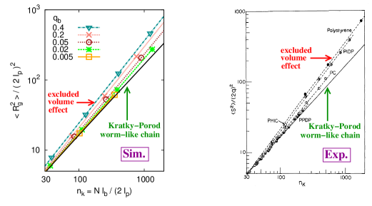
Figure 1: (a) Log-log plot of normalized gyration radius square ⟨Rg2⟩/(2​ℓp)2delimited-⟨⟩superscriptsubscript𝑅𝑔2superscript2subscriptℓ𝑝2\langle R_{g}^{2}\rangle/(2\ell_{p})^{2} versus the number of Kuhn segments, for the range 30≀nK≀300030subscript𝑛𝐾300030\leq n_{K}\leq 3000, for chains of widely varying stiffness, and comparison to corresponding experimental data (b), taken from Norisuye and FujitaΒ 12 . The full straight line is the Kratky-Porod model, Eq.Β (24).

For stronger forces (corresponding to ΞΎp<R0subscriptπœ‰π‘subscript𝑅0\xi_{p}<R_{0}) the Kratky-Porod results, Eqs.Β (56), (57), are expected to become valid. In the Pincus blob regime, also nontrivial power laws for the fluctuations ⟨X2βŸ©βˆ’βŸ¨X⟩2delimited-⟨⟩superscript𝑋2superscriptdelimited-βŸ¨βŸ©π‘‹2\langle X^{2}\rangle-\langle X\rangle^{2} and the transverse linear dimensions are predictedΒ 44

⟨X2βŸ©βˆ’βŸ¨X⟩2∝⟨RβŠ₯2⟩∝(f​ℓp/kB​T)1/Ξ½βˆ’2.proportional-todelimited-⟨⟩superscript𝑋2superscriptdelimited-βŸ¨βŸ©π‘‹2delimited-⟨⟩superscriptsubscript𝑅bottom2proportional-tosuperscript𝑓subscriptℓ𝑝subscriptπ‘˜π΅π‘‡1𝜈2\langle X^{2}\rangle-\langle X\rangle^{2}\propto\langle R_{\bot}^{2}\rangle\propto(f\ell_{p}/k_{B}T)^{1/\nu-2}\,. (63)

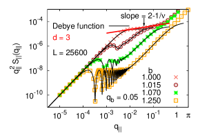
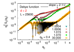
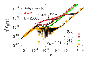
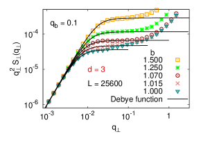
Since we are not aware of any treatment of the structure factor of the Kratky-Porod model under stretch, we shall use Eqs.Β (48), (49) also for semiflexible chains (but using the numerical results for ⟨X⟩delimited-βŸ¨βŸ©π‘‹\langle X\rangle and ⟨X2βŸ©βˆ’βŸ¨X⟩2,⟨Rg,βŠ₯2⟩delimited-⟨⟩superscript𝑋2superscriptdelimited-βŸ¨βŸ©π‘‹2delimited-⟨⟩superscriptsubscript𝑅𝑔bottom2\langle X^{2}\rangle-\langle X\rangle^{2},\;\langle R_{g,\bot}^{2}\rangle, rather than theoretical predictions).

(a)Refer to captionΒ Β Β Β  (b)Refer to caption
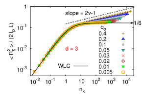
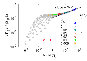
Figure 2: (a) Log-log plot of ⟨Rg2⟩/(2​ℓp​L)delimited-⟨⟩superscriptsubscript𝑅𝑔22subscriptℓ𝑝𝐿\langle R_{g}^{2}\rangle/(2\ell_{p}L) versus nKsubscript𝑛𝐾n_{K} for d=3𝑑3d=3, and including data for widely varying persistence lengths. Note that the worm-like chain result, WLC (Eq.Β (24)), describes correctly the crossover from rods to coils, but not the onset of excluded volume effects. (b) Same as (a), but choosing N/Nβˆ—β€‹(qb)𝑁superscript𝑁subscriptπ‘žπ‘N/N^{*}(q_{b}) as an abscissa variable (Nβˆ—β€‹(qb)superscript𝑁subscriptπ‘žπ‘N^{*}(q_{b}) was already estimated for a similar scaling plot for the mean square end-to-end distance, cf. Fig.Β 7b of Ref.Β 13 ). Here L=N​ℓb𝐿𝑁subscriptℓ𝑏L=N\ell_{b}.
Refer to caption
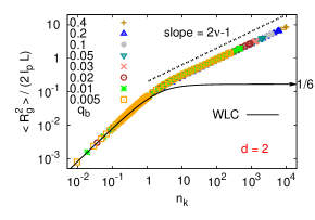
Figure 3: Log-log plot of ⟨Rg2⟩/(2​ℓp​L)delimited-⟨⟩superscriptsubscript𝑅𝑔22subscriptℓ𝑝𝐿\langle R_{g}^{2}\rangle/(2\ell_{p}L) versus nKsubscript𝑛𝐾n_{K} for d=2𝑑2d=2, including data for widely varying persistence lengths. Note that in d=2𝑑2d=2 there occurs a direct crossover from rods to SAWs, an intermediate Gaussian regime in absent.

(a)Refer to captionΒ Β Β Β  (b)Refer to caption

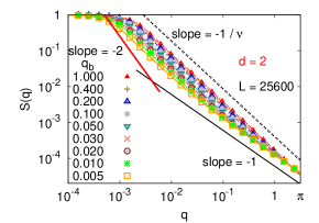
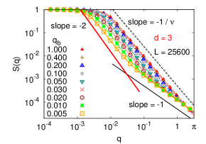
Figure 4: Structure factor S​(q)π‘†π‘žS(q) plotted qπ‘žq, on log-log- scales, for d=2𝑑2d=2 (a) and d=3𝑑3d=3 (b); only data for L=25600𝐿25600L=25600 are shown, but many different choices of the stiffness parameter qbsubscriptπ‘žπ‘q_{b} are included. The straight lines indicate the rod-like behavior at large qπ‘žq (slope =βˆ’1absent1=-1) and the SAW behavior for flexible chains (slope =βˆ’1/Ξ½absent1𝜈=-1/\nu). Also the slope expected in the Gaussian regime is included (slope =βˆ’2absent2=-2). Only data up to q=Ο€π‘žπœ‹q=\pi have been included (larger qπ‘žq cannot be studied due to the lattice character of our model).

(a)Refer to captionΒ Β Β Β  (b)Refer to caption

(c)Refer to caption

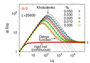
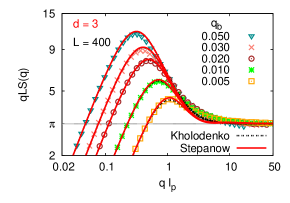
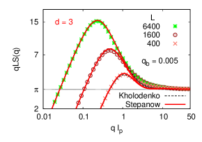
Figure 5: (a) Rescaled structure factor q​L​S​(q)π‘žπΏπ‘†π‘žqLS(q) plotted against L​qπΏπ‘žLq for d=3𝑑3d=3 and L=25600𝐿25600L=25600, including 5 choices of the stiffness. The result for Gaussian chains (Debye function) and for continuous rigid rods (for which q​L​S​(q)β†’Ο€β†’π‘žπΏπ‘†π‘žπœ‹qLS(q)\rightarrow\pi for large qπ‘žq. cf.Β Eq.Β (28)) are included for comparison. Also predictions obtained from the formulas proposed by Kholodenko {Eqs.Β (31)-(36)} are shown. (b) Rescaled structure factor q​L​S​(q)π‘žπΏπ‘†π‘žqLS(q) plotted against q​ℓpπ‘žsubscriptℓ𝑝q\ell_{p} for d=3𝑑3d=3 and for L=400𝐿400L=400, including both the predictions due to StepanowΒ 271 and Kholodenko {Eq.Β (31) - (36)}, which are essentially indistinguishable on the scale of the figure. (c) Same as (b), but for 3 different choices of L𝐿L for qb=0.005subscriptπ‘žπ‘0.005q_{b}=0.005.

(a)Refer to captionΒ Β Β Β  (b)Refer to caption

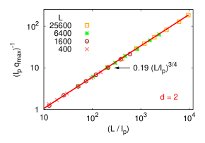
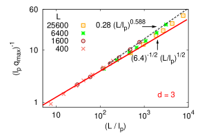
Figure 6: Log-log plot of the inverse position of the maximum in the Kratky plot, (β„“p​qmax)βˆ’1superscriptsubscriptℓ𝑝subscriptπ‘žmax1(\ell_{p}q_{\rm max})^{-1}, versus the rescaled contour length L/β„“p𝐿subscriptℓ𝑝L/\ell_{p}, for d=2𝑑2d=2 (a) and d=3𝑑3d=3 (b). The full straight line included in (a) is described by the equation 0.19​(L/β„“p)3/40.19superscript𝐿subscriptℓ𝑝340.19(L/\ell_{p})^{3/4}. In case (b), two straight lines with slope Ξ½=1/2𝜈12\nu=1/2 and Ξ½=0.588𝜈0.588\nu=0.588 are included, to illustrate the crossover. In both cases the persistence length β„“psubscriptℓ𝑝\ell_{p} is varied over a wide range, and the contour lengths chosen are L=400𝐿400L=400, 160016001600, 640064006400 and 256002560025600, as indicated.

(a)Refer to captionΒ Β Β Β  (b)Refer to caption

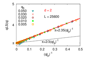
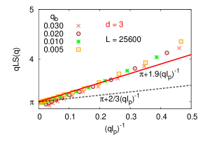
Figure 7: Plot of q​L​S​(q)π‘žπΏπ‘†π‘žqLS(q) vs.Β (q​Lp)βˆ’1superscriptπ‘žsubscript𝐿𝑝1(qL_{p})^{-1}, for d=2𝑑2d=2 (a) and d=3𝑑3d=3 (b). All data are for L=25600𝐿25600L=25600 only, and many different choices of qbsubscriptπ‘žπ‘q_{b}, as indicated. In each case, two straight lines are shown: the result of des CloizeauxΒ 18 , Eq.Β (1), q​L​S​(q)=Ο€+(2/3)​(q​ℓp)βˆ’1π‘žπΏπ‘†π‘žπœ‹23superscriptπ‘žsubscriptℓ𝑝1qLS(q)=\pi+(2/3)(q\ell_{p})^{-1}, and empirical fits, q​L​S​(q)=Ο€+2.35​(q​ℓp)βˆ’1π‘žπΏπ‘†π‘žπœ‹2.35superscriptπ‘žsubscriptℓ𝑝1qLS(q)=\pi+2.35(q\ell_{p})^{-1} for d=2𝑑2d=2 and q​L​S​(q)=Ο€+1.9​(q​ℓp)βˆ’1π‘žπΏπ‘†π‘žπœ‹1.9superscriptπ‘žsubscriptℓ𝑝1qLS(q)=\pi+1.9(q\ell_{p})^{-1} for d=3𝑑3d=3, respectively.

III Model and Simulation Technique

Our model is the standard self-avoiding walk (SAW) on the square and simple cubic lattices, effective monomers being described by occupied lattice sites, connected by bonds. Each site can be taken only once, and thus we realize the excluded volume interaction. The lattice spacing henceforth is our unit of length, β„“b=1subscriptℓ𝑏1\ell_{b}=1. We introduce an energy Ο΅bsubscriptitalic-ϡ𝑏\epsilon_{b} for any kink the walk takes (by an angle of Β±90∘plus-or-minussuperscript90\pm 90^{\circ}). Any such kink introduces hence a factor qb=exp⁑(βˆ’Ο΅b/kB​T)subscriptπ‘žπ‘subscriptitalic-ϡ𝑏subscriptπ‘˜π΅π‘‡q_{b}=\exp(-\epsilon_{b}/k_{B}T) to the statistical weight of the walk.

In the presence of a force f𝑓f coupling to the extension X𝑋X of the chain in x-direction, the statistical weight gets another factor bXsuperscript𝑏𝑋b^{X}, with b=exp⁑(f/kB​T)𝑏𝑓subscriptπ‘˜π΅π‘‡b=\exp(f/k_{B}T). Then the partition function of a SAW with N𝑁N bonds (i.e., N+1𝑁1N+1 effective monomers) and Nbendsubscript𝑁bendN_{\rm bend} local kinks becomes

ZN,Nbend​(qb,b)=βˆ‘config.C​(N,Nbend,X)​qbNbend​bXsubscript𝑍𝑁subscript𝑁bendsubscriptπ‘žπ‘π‘subscriptconfig.𝐢𝑁subscript𝑁bend𝑋superscriptsubscriptπ‘žπ‘subscript𝑁bendsuperscript𝑏𝑋Z_{N,N_{\rm bend}}(q_{b},b)=\sum\limits_{\textrm{config.}}C(N,N_{\rm bend},X)q_{b}^{N_{\rm bend}}b^{X} (64)

By the pruned-enriched Rosenbluth method (PERM) it is possible to obtain estimates of the partition function and quantities derived from it (e.g. ⟨X⟩,⟨X2⟩)\langle X\rangle,\langle X^{2}\rangle) and additional averages such as S​(q)π‘†π‘žS(q), using chain lengths up to N=25600𝑁25600N=25600. Both the chain stiffness and the force f𝑓f have been varied over a wide range; for qb=1subscriptπ‘žπ‘1q_{b}=1 one has fully flexible self-avoiding random walks, while for qb=0.005subscriptπ‘žπ‘0.005q_{b}=0.005 the persistence length (computed from Eq.Β (21)) is of the order of 120120120 in d=2𝑑2d=2 and 525252 in d=3𝑑3d=3 (Table I lists our corresponding estimates). For technical details on the implementation of the algorithm, we refer to the literatureΒ 13 .

IV Results for the scattering function of unstretched chains

We start with our data for the mean square gyration radius ⟨Rg2⟩delimited-⟨⟩superscriptsubscript𝑅𝑔2\langle R_{g}^{2}\rangle, normalized by the square of the Kuhn length β„“K=2​ℓpsubscriptℓ𝐾2subscriptℓ𝑝\ell_{K}=2\ell_{p}, plotted vs.Β the number of Kuhn segments nK=L/β„“K=N​ℓb/(2​ℓp)subscript𝑛𝐾𝐿subscriptℓ𝐾𝑁subscriptℓ𝑏2subscriptℓ𝑝n_{K}=L/\ell_{K}=N\ell_{b}/(2\ell_{p}), Fig.Β 1a since this was the representation chosen for the experimental data of Norisuye and FujitaΒ 12 , which we reproduce in Fig.Β 1b. Both diagrams show the same range of abscissa (30≀nK≀3000)30subscript𝑛𝐾3000(30\leq n_{K}\leq 3000) and ordinate (5<⟨Rg2⟩/(2​ℓp)2<1000)5delimited-⟨⟩superscriptsubscript𝑅𝑔2superscript2subscriptℓ𝑝21000(5<\langle R_{g}^{2}\rangle/(2\ell_{p})^{2}<1000). The qualitative similarity between both simulation and experiment is striking. Since only the regime of rather large nKsubscript𝑛𝐾n_{K} is shown, the crossover from rods to Gaussian chains is not included (the full straight line represents the Gaussian chain behavior, as described by Eq.Β (24) for nK=(1/2)​np≫1subscript𝑛𝐾12subscript𝑛𝑝much-greater-than1n_{K}=(1/2)n_{p}\gg 1). One can see that Eq.Β (24) works for very stiff chains and not too large nKsubscript𝑛𝐾n_{K}, while for large nKsubscript𝑛𝐾n_{K} systematic deviations occur, which can be attributed to excluded volume effects. Both the simulation and the experiment include data for widely varying persistence lengths (in the experiment, this could only be achieved by combining data for chemically different polymers in this plot). From their results (see Fig.Β 1b) the experimentalists concluded that the excluded volume effects set in for nK>50subscript𝑛𝐾50n_{K}>50, irrespective of the precise value of the persistence length.

However, this latter conclusion needs to be questioned: in fact, for large nKsubscript𝑛𝐾n_{K} the data do not superimpose in this representation for different choices of β„“psubscriptℓ𝑝\ell_{p}, indicating that the behavior is more complicated. To elucidate this, we take out the leading power law in the Gaussian coil regime, plotting ⟨Rg2⟩/(β„“p​L)delimited-⟨⟩superscriptsubscript𝑅𝑔2subscriptℓ𝑝𝐿\langle R_{g}^{2}\rangle/(\ell_{p}L) versus nKsubscript𝑛𝐾n_{K} over the full range (Fig.Β 2a). One sees that nice scaling behavior occurs with respect to the crossover from rigid rods to Gaussian coils; in this regime, Eq.Β (24) works in d=3𝑑3d=3. However, now one can see rather clearly that the crossover from Gaussian coils to SAWs does not scale in this representation: rather for large nKsubscript𝑛𝐾n_{K} the curves β€œsplay out”, the larger β„“psubscriptℓ𝑝\ell_{p} the longer the data follow Eq.Β (24), before an onset of excluded volume effects can be seen. This behavior has already been studied in Ref.Β 13 with respect to the end-to-end distance. Empirically, it was found that scaling N𝑁N with Nβˆ—superscript𝑁N^{*}, where Nβˆ—βˆβ„“p2.5proportional-tosuperscript𝑁superscriptsubscriptℓ𝑝2.5N^{*}\propto\ell_{p}^{2.5} rather than Nβˆ—=β„“psuperscript𝑁subscriptℓ𝑝N^{*}=\ell_{p}. Fig.Β 2b shows that a master curve results as an envelope of the curves for individual β„“psubscriptℓ𝑝\ell_{p}. We also recall, that Flory arguments predict Nβˆ—βˆβ„“p3proportional-tosuperscript𝑁superscriptsubscriptℓ𝑝3N^{*}\propto\ell_{p}^{3}, cf. Eq.Β (45) and the subsequent discussion. The data in Fig.Β 2 are fully analogous to our data on the end-to-end distance that were discussed recently elsewhereΒ 13 . In d=2𝑑2d=2, however, the behavior is clearly simpler (Fig.Β 3): there occurs a single crossover from rods to d=2𝑑2d=2 SAWs, and a regime where the Kratky-Porod worm-like chain model presents a faithful description of the data is absent. These results for ⟨Rg2⟩delimited-⟨⟩superscriptsubscript𝑅𝑔2\langle R_{g}^{2}\rangle confirm our earlier analogous findingsΒ 13 for ⟨Re2⟩delimited-⟨⟩superscriptsubscript𝑅𝑒2\langle R_{e}^{2}\rangle.

Fig.Β 4 shows some of our raw data for the structure factor S​(q)π‘†π‘žS(q). For small qπ‘žq, one recognizes the Guinier regime, S​(q)β‰ˆexp⁑(βˆ’q2β€‹βŸ¨Rg2⟩/3)β‰ˆ1βˆ’q2β€‹βŸ¨Rg2⟩/3π‘†π‘žsuperscriptπ‘ž2delimited-⟨⟩superscriptsubscript𝑅𝑔231superscriptπ‘ž2delimited-⟨⟩superscriptsubscript𝑅𝑔23S(q)\approx\exp(-q^{2}\langle R_{g}^{2}\rangle/3)\approx 1-q^{2}\langle R_{g}^{2}\rangle/3, and then a crossover occurs to the power law of SAWs or of Gaussian chains (the latter is seen clearly only for d=3𝑑3d=3 and very stiff chains). At large qπ‘žq and stiff chains, the expected qβˆ’1superscriptπ‘ž1q^{-1} behavior is in fact compatible with the data.

It turns out that an analysis of S​(q)π‘†π‘žS(q) in the form of Kratky plots (Eq.Β (37)) is more illuminating, cf. Fig.Β 5: The location of the maximum in the Kratky plot, as discussed in Eqs.Β (38), (39), is easily identified, and it shows the expected scaling with L/β„“p𝐿subscriptℓ𝑝L/\ell_{p} both in d=3𝑑3d=3 and in d=2𝑑2d=2 (Fig.Β 6). In d=3𝑑3d=3, one notes that with increasing L/β„“p𝐿subscriptℓ𝑝L/\ell_{p} a crossover from Gaussian behavior to SAW behavior occurs. Our data also confirm that for rather stiff chains in d=3𝑑3d=3 both the Kholodenko and the Stepanow theories describe S​(q)π‘†π‘žS(q) very accurately. Note that Fig.Β 5b refers to rather short chains, for which strong effects due to excluded volume interactions are not yet expected, and hence the good agreement with the theories is not surprising.

Another issue of interest is the behavior q​L​S​(q)π‘žπΏπ‘†π‘žqLS(q) in the rigid rod limit, where one clearly notes the approach to Ο€πœ‹\pi (Fig.Β 5). Can we then use S​(q)π‘†π‘žS(q) in this region, applying the des Cloizeaux formula {Eq.Β (1)} to extract quantitatively reliable estimates for the persistence length β„“psubscriptℓ𝑝\ell_{p} from a plot of q​L​S​(q)π‘žπΏπ‘†π‘žqLS(q) versus 1/q1π‘ž1/q ? Fig.Β 7 suggests that although a regime occurs where the variation is linear in (q​ℓp)βˆ’1superscriptπ‘žsubscriptℓ𝑝1(q\ell_{p})^{-1}, the coefficient of this linear variation is inconsistent with the des Cloizeaux result. We have no final answer to offer to explain this discrepancy; we suspect that in the regime where qβˆ’1superscriptπ‘ž1q^{-1} and β„“psubscriptℓ𝑝\ell_{p} are of the same order, the discreteness of our lattice model (opposed to the Kratky-Porod continuum model) might matter.

V Results for the scattering function of chains under stretch

While for unstretched chains it is only ⟨Rg2⟩delimited-⟨⟩superscriptsubscript𝑅𝑔2\langle R_{g}^{2}\rangle as a measure of the linear dimension of the whole chain which is relevant (Figs.Β 1-3), for chains under the action of stretching forces anisotropy of the conformation of the chain comes into play. However, from the small qπ‘žq expansion of Eqs.Β (4), (5) one can show straightforwardly that S||​(q||)S_{||}(q_{||}) yields information on ⟨Rg,||2⟩\langle R_{g,||}^{2}\rangle and SβŠ₯​(qβŠ₯)subscript𝑆bottomsubscriptπ‘žbottomS_{\bot}(q_{\bot}) on ⟨Rg,βŠ₯2⟩delimited-⟨⟩superscriptsubscript𝑅𝑔bottom2\langle R_{g,\bot}^{2}\rangle cf. Eqs.Β (14) and (15). Since for larger q||q_{||} where also the extension ⟨X⟩delimited-βŸ¨βŸ©π‘‹\langle X\rangle of the chain along the direction of the force enters the description of the scattering, we begin with a discussion of these linear dimensions and describe their variation as a function of the force f𝑓f (for a more detailed discussion and related results, we refer the reader to Ref.Β 13 ).

(a)Refer to captionΒ Β Β Β  (b)Refer to caption

(c)Refer to captionΒ Β Β Β  (d)Refer to caption

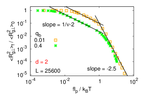
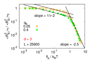
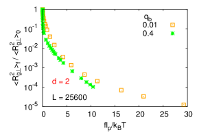
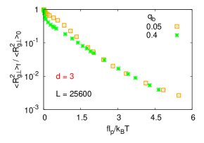
Figure 8: Log-log plot of ⟨Rg,βŠ₯2⟩/⟨Rg,βŠ₯2⟩0delimited-⟨⟩superscriptsubscript𝑅𝑔bottom2subscriptdelimited-⟨⟩superscriptsubscript𝑅𝑔bottom20\langle R_{g,\bot}^{2}\rangle/\langle R_{g,\bot}^{2}\rangle_{0} vs.Β f​ℓp/kB​T𝑓subscriptℓ𝑝subscriptπ‘˜π΅π‘‡f\ell_{p}/k_{B}T, for d=2𝑑2d=2 (a) and for d=3𝑑3d=3 (b), using L=N​ℓb=25600𝐿𝑁subscriptℓ𝑏25600L=N\ell_{b}=25600 in both cases, for two choices of qbsubscriptπ‘žπ‘q_{b}. In parts (c,d) the same data as in (a,b) for large f​ℓp/kB​T𝑓subscriptℓ𝑝subscriptπ‘˜π΅π‘‡f\ell_{p}/k_{B}T are replotted choosing a linear scale for f​ℓp/kB​T𝑓subscriptℓ𝑝subscriptπ‘˜π΅π‘‡f\ell_{p}/k_{B}T, to show that the behavior is compatible with an exponential decay in d=3𝑑3d=3.

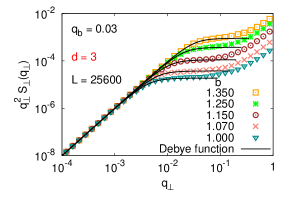
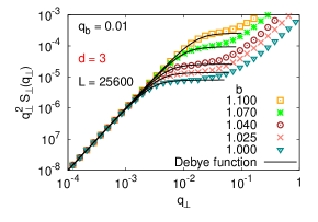
Fig.Β 8 shows typical data of ⟨Rg,βŠ₯2⟩delimited-⟨⟩superscriptsubscript𝑅𝑔bottom2\langle R_{g,\bot}^{2}\rangle versus f​ℓp/kB​T𝑓subscriptℓ𝑝subscriptπ‘˜π΅π‘‡f\ell_{p}/k_{B}T, both for rather flexible chains (qb=0.4)subscriptπ‘žπ‘0.4(q_{b}=0.4) and for rather stiff chains (qb=0.01(q_{b}=0.01 in d=2𝑑2d=2, qb=0.05subscriptπ‘žπ‘0.05q_{b}=0.05 in d=3𝑑3d=3, respectively). We recognize three regimes: for very small forces ⟨Rg,βŠ₯2βŸ©β‰ˆβŸ¨Rg,βŠ₯2⟩0delimited-⟨⟩superscriptsubscript𝑅𝑔bottom2subscriptdelimited-⟨⟩superscriptsubscript𝑅𝑔bottom20\langle R_{g,\bot}^{2}\rangle\approx\langle R_{g,\bot}^{2}\rangle_{0}, the unperturbed value in the absence of forces. In this linear response regime, the force orients the coil without deforming it. Then we recognize a regime where ⟨Rg,βŠ₯2⟩delimited-⟨⟩superscriptsubscript𝑅𝑔bottom2\langle R_{g,\bot}^{2}\rangle decreases according to a power law, namely Eq.Β (63). This power law holds in the regime where the radius of the Pincus blob, ΞΎp=kB​T/fsubscriptπœ‰π‘subscriptπ‘˜π΅π‘‡π‘“\xi_{p}=k_{B}T/f, is smaller than the unperturbed radius, but much larger than the persistence length β„“psubscriptℓ𝑝\ell_{p} itself. Thus this is the analog of the β€œPincus blob” law that yields another power law for the extension vs.Β force curve, Eq.Β (61). The physical picture invoked here for the chain is an elastic string of Pincus blobs, ⟨Rg,βŠ₯2⟩delimited-⟨⟩superscriptsubscript𝑅𝑔bottom2\langle R_{g,\bot}^{2}\rangle describing the mean square displacement of this string in transverse directions. As one can see from Fig.Β 8, the data indeed are compatible with the predicted power law in d=2𝑑2d=2, and in d=3𝑑3d=3 at least for the flexible chains. For stiff chains in d=3𝑑3d=3, the regime where Eq.Β (63) holds is more restricted, since the Kratky-Porod regime has a more extended regime of validity, effects due to Pincus blobs can only be detected in a regime ⟨Rg,βŠ₯2⟩01/2>ΞΎp>Rβˆ—βˆβ„“p2/Dsubscriptsuperscriptdelimited-⟨⟩superscriptsubscript𝑅𝑔bottom2120subscriptπœ‰π‘superscript𝑅proportional-tosuperscriptsubscriptℓ𝑝2𝐷\langle R_{g,\bot}^{2}\rangle^{1/2}_{0}>\xi_{p}>R^{*}\propto\ell_{p}^{2}/D, cf. Eq.Β (62)Β 13 . Therefore we have not included very stiff chains in Fig.Β 8b (for qb=0.005subscriptπ‘žπ‘0.005q_{b}=0.005, leading to β„“pβ‰ˆ52​ℓbsubscriptℓ𝑝52subscriptℓ𝑏\ell_{p}\approx 52\ell_{b}, excluded volume effects, which also are responsible for the existence of Pincus blobs, could even for chains as long as N=25600𝑁25600N=25600 hardly be detected in the chain linear dimensions in the absence of a force, cf. Figs.Β 1-3). So this failure to detect Pincus blobs for very stiff long chains in d=3𝑑3d=3 dimensions is hardly surprising (although Eq.Β (63) ultimatively will become valid as Nβ†’βˆžβ†’π‘N\rightarrow\infty, irrespective how large β„“psubscriptℓ𝑝\ell_{p} is).

Another interesting behavior is the apparent power law, ⟨Rg,βŠ₯2⟩∝(f​ℓp/kB​T)βˆ’2.5proportional-todelimited-⟨⟩superscriptsubscript𝑅𝑔bottom2superscript𝑓subscriptℓ𝑝subscriptπ‘˜π΅π‘‡2.5\langle R_{g,\bot}^{2}\rangle\propto(f\ell_{p}/k_{B}T)^{-2.5}, seen for f​ℓp/kB​T>1𝑓subscriptℓ𝑝subscriptπ‘˜π΅π‘‡1f\ell_{p}/k_{B}T>1. However, we warn the reader to take this seriously: a closer look reveals a slight but systematic curvature, and a plot versus f​ℓp/kB​T𝑓subscriptℓ𝑝subscriptπ‘˜π΅π‘‡f\ell_{p}/k_{B}T on a linear rather than a logarithmic scale reveals that this apparent power law is nothing but the onset of an exponential decay (Figs.Β 8c,d): indeed, already from the partition function, Eq.Β (64) we recognize that for large forces the chains will be stretched out almost completely like rigid rods, and the few remaining kinks are suppressed exponentially when f​ℓp/kB​T≫1much-greater-than𝑓subscriptℓ𝑝subscriptπ‘˜π΅π‘‡1f\ell_{p}/k_{B}T\gg 1.

(a)Refer to captionΒ Β Β Β  (b)Refer to caption

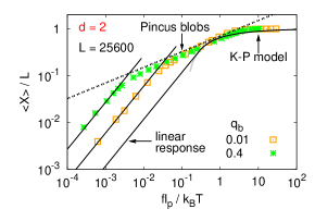
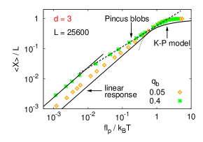
Figure 9: Log-log plot of the relative extension ⟨X⟩/Ldelimited-βŸ¨βŸ©π‘‹πΏ\langle X\rangle/L versus the scaled force f​ℓp/kB​T𝑓subscriptℓ𝑝subscriptπ‘˜π΅π‘‡f\ell_{p}/k_{B}T for L=25600𝐿25600L=25600 in d=2𝑑2d=2 (a) and d=3𝑑3d=3, for the same choices of qbsubscriptπ‘žπ‘q_{b} as shown in Fig.Β 8. The straight lines indicate the linear response regime and the Pincus-blob regime, respectively {Eq.Β (61)}. In neither case has the Kratky-Porod model (curves labeled as K-P-model, cf.Β Eqs.Β (56), (57)) a well-defined regime of validity (this is expected since for large f​ℓp/kB​T𝑓subscriptℓ𝑝subscriptπ‘˜π΅π‘‡f\ell_{p}/k_{B}T the approach to saturation, ⟨X⟩/Lβ†’1β†’delimited-βŸ¨βŸ©π‘‹πΏ1\langle X\rangle/L\rightarrow 1, is exponentially fast rather than proportional to (kB​T/f​ℓp)1/2superscriptsubscriptπ‘˜π΅π‘‡π‘“subscriptℓ𝑝12(k_{B}T/f\ell_{p})^{1/2}, cf. Fig.Β 8).

(a)Refer to captionΒ Β Β Β  (b)Refer to caption

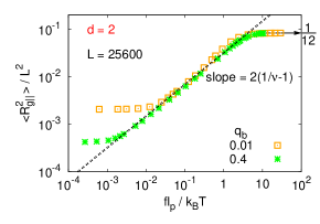
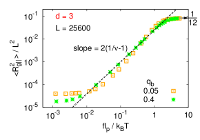
Figure 10: Log-log plot of the parallel component ⟨Rg,||2⟩/L2\langle R_{g,||}^{2}\rangle/L^{2} vs.Β f​ℓp/kB​T𝑓subscriptℓ𝑝subscriptπ‘˜π΅π‘‡f\ell_{p}/k_{B}T, for the same parameters as in Figs.Β 8, 9. Straight lines indicate the Pincus blob regime. Part (a) refers to d=2𝑑2d=2, part (b) to d=3𝑑3d=3.

For completeness, we show the corresponding simulation data for the relative extension ⟨X⟩/Ldelimited-βŸ¨βŸ©π‘‹πΏ\langle X\rangle/L vs.Β f​ℓp/kB​T𝑓subscriptℓ𝑝subscriptπ‘˜π΅π‘‡f\ell_{p}/k_{B}T in Fig.Β 9 (related more extensive data for other values of L𝐿L and qbsubscriptπ‘žπ‘q_{b} can be found in Ref.Β 13 ), and in Fig.Β 10 we present the corresponding data for the longitudinal component ⟨Rg,||2⟩/L2\langle R_{g,||}^{2}\rangle/L^{2} of the gyration radius in the direction of the force. While for very small forces one expects a nonzero plateau (unlike ⟨X⟩/Ldelimited-βŸ¨βŸ©π‘‹πΏ\langle X\rangle/L, which vanishes as fβ†’0→𝑓0f\rightarrow 0), corresponding to the gyration radius square component of an unstretched chain, for large f𝑓f another plateau means that the chain has been stretched out fully to a rod of length L𝐿L. In between these two plateaus, the Pincus blob behavior is seen rather clearly, for the flexible chains.

(a)Refer to captionΒ Β Β Β  (b)Refer to caption
(c)Refer to captionΒ Β Β Β  (d)Refer to caption

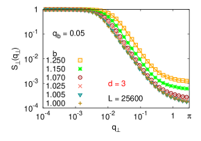
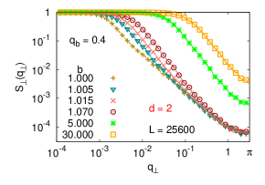
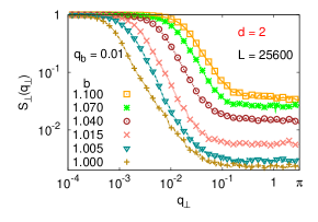
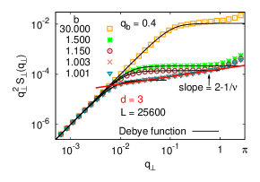
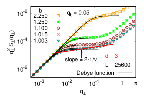
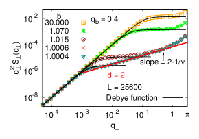
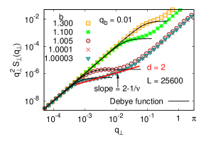
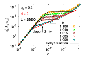
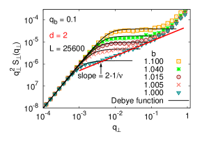
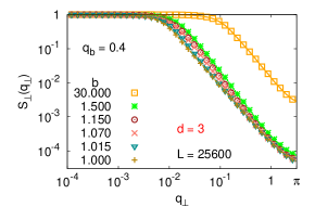
Figure 11: Log-log plot of the structure factor SβŠ₯​(qβŠ₯)subscript𝑆bottomsubscriptπ‘žbottomS_{\bot}(q_{\bot}) vs.Β qβŠ₯subscriptπ‘žbottomq_{\bot} for d=3𝑑3d=3 and two choices of the stiffness parameter qbsubscriptπ‘žπ‘q_{b}, qb=0.4subscriptπ‘žπ‘0.4q_{b}=0.4 (a) and qb=0.05subscriptπ‘žπ‘0.05q_{b}=0.05 (b), and also for d=2𝑑2d=2 and two choices of qbsubscriptπ‘žπ‘q_{b}, namely qb=0.4subscriptπ‘žπ‘0.4q_{b}=0.4 (c) and qb=0.01subscriptπ‘žπ‘0.01q_{b}=0.01. In each case several choices of b=exp⁑(f/kB​T)𝑏𝑓subscriptπ‘˜π΅π‘‡b=\exp(f/k_{B}T) are included, as indicated. Chain length is L=25600𝐿25600L=25600 throughout.

(a)Refer to captionΒ Β Β Β  (b)Refer to caption

(c)Refer to captionΒ Β Β Β  (d)Refer to caption

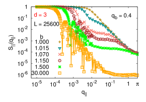
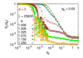
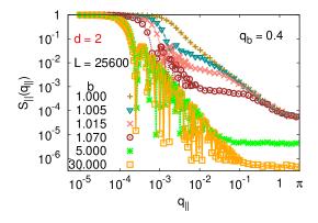
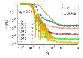
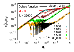
Figure 12: Log-log plot of the structure factor S||​(q||)S_{||}(q_{||}) vs.Β q||q_{||} for d=3𝑑3d=3 and two choices of the stiffness parameter qbsubscriptπ‘žπ‘q_{b}, qb=0.4subscriptπ‘žπ‘0.4q_{b}=0.4 (a) and qb=0.05subscriptπ‘žπ‘0.05q_{b}=0.05 (b), and also for d=2𝑑2d=2 and two choices of qbsubscriptπ‘žπ‘q_{b}, namely qb=0.4subscriptπ‘žπ‘0.4q_{b}=0.4 (c) and qb=0.01subscriptπ‘žπ‘0.01q_{b}=0.01 (d). In each case several choices of b=exp⁑(f/kB​T)𝑏𝑓subscriptπ‘˜π΅π‘‡b=\exp(f/k_{B}T) are included. Chain length is L=25600𝐿25600L=25600 throughout.

Fig.Β 11 now shows typical data for SβŠ₯​(qβŠ₯)subscript𝑆bottomsubscriptπ‘žbottomS_{\bot}(q_{\bot}) vs.Β qβŠ₯subscriptπ‘žbottomq_{\bot} and Fig.Β 12 the corresponding data for S||​(q||)S_{||}(q_{||}) vs.Β q||q_{||}, focusing again on those selected values of qbsubscriptπ‘žπ‘q_{b} that were used already in Figs.Β 8-10. As expected from Eq.Β (49), the perpendicular structure factor is similar to the case without stretching force; the plateau at small qπ‘žq, where SβŠ₯​(qβŠ₯)subscript𝑆bottomsubscriptπ‘žbottomS_{\bot}(q_{\bot}) deviates only very little from unity, gets more extended with increasing f𝑓f, reflecting the decrease of ⟨Rg,βŠ₯2⟩delimited-⟨⟩superscriptsubscript𝑅𝑔bottom2\langle R_{g,\bot}^{2}\rangle with f𝑓f (Fig.Β 8). This decrease, of course, is more pronounced for stiff chains than for flexible chains at the same value of f𝑓f, since we have seen (see Fig.Β 8 and the discussions in Ref.Β 13 ) that the proper control variable is not f/kB​T𝑓subscriptπ‘˜π΅π‘‡f/k_{B}T but rather f​ℓp/kB​T𝑓subscriptℓ𝑝subscriptπ‘˜π΅π‘‡f\ell_{p}/k_{B}T. A further remarkable feature is the fact, that the power law-like decay of SβŠ₯​(qβŠ₯)subscript𝑆bottomsubscriptπ‘žbottomS_{\bot}(q_{\bot}) with qβŠ₯subscriptπ‘žbottomq_{\bot}, that for flexible chains can be observed until SβŠ₯​(qβŠ₯)subscript𝑆bottomsubscriptπ‘žbottomS_{\bot}(q_{\bot}) has decayed up to SβŠ₯​(qβŠ₯)β‰ˆ10βˆ’4subscript𝑆bottomsubscriptπ‘žbottomsuperscript104S_{\bot}(q_{\bot})\approx 10^{-4} as b<1.5𝑏1.5b<1.5, for stiff chains extends only to SβŠ₯​(qβŠ₯)β‰ˆ10βˆ’3subscript𝑆bottomsubscriptπ‘žbottomsuperscript103S_{\bot}(q_{\bot})\approx 10^{-3} in d=3𝑑3d=3 and SβŠ₯​(qβŠ₯)β‰ˆ10βˆ’2subscript𝑆bottomsubscriptπ‘žbottomsuperscript102S_{\bot}(q_{\bot})\approx 10^{-2} in d=2𝑑2d=2, respectively. As expected, the theory of Benoit et al.Β 30 which extended the description of scattering from Gaussian chains to elastic stretching deformations, can only be applied if qβŠ₯​ℓpβ‰ͺ1much-less-thansubscriptπ‘žbottomsubscriptℓ𝑝1q_{\bot}\ell_{p}\ll 1, and when ⟨Rg,βŠ₯2⟩delimited-⟨⟩superscriptsubscript𝑅𝑔bottom2\langle R_{g,\bot}^{2}\rangle exceeds β„“p2superscriptsubscriptℓ𝑝2\ell_{p}^{2} only by few orders of magnitudes, the applicability of Eq.Β (49) is correspondingly restricted. In fact, noting that, for qb=0.05subscriptπ‘žπ‘0.05q_{b}=0.05, β„“p/β„“bβ‰ˆ5.9subscriptℓ𝑝subscriptℓ𝑏5.9\ell_{p}/\ell_{b}\approx 5.9, we conclude that b=1.5𝑏1.5b=1.5 means f​ℓp/kB​Tβ‰ˆ2.4𝑓subscriptℓ𝑝subscriptπ‘˜π΅π‘‡2.4f\ell_{p}/k_{B}T\approx 2.4, and Fig.Β 8 shows that in this case indeed ⟨Rg,βŠ₯2⟩delimited-⟨⟩superscriptsubscript𝑅𝑔bottom2\langle R_{g,\bot}^{2}\rangle is about an order of magnitude smaller than for f=0𝑓0f=0. Assuming that one can represent a stiff chain as a sequence of rods of length β„“psubscriptℓ𝑝\ell_{p} such that np​ℓp=N​ℓbsubscript𝑛𝑝subscriptℓ𝑝𝑁subscriptℓ𝑏n_{p}\ell_{p}=N\ell_{b}, and stating in the spirit of Eq.Β (II.1) that at large qβŠ₯subscriptπ‘žbottomq_{\bot} interference effects of different rods can be neglected, one would expect that for qβŠ₯​ℓpβ‰ˆ1subscriptπ‘žbottomsubscriptℓ𝑝1q_{\bot}\ell_{p}\approx 1 one obtains a scattering of the order of SβŠ₯​(qβŠ₯)β‰ˆnpβˆ’1subscript𝑆bottomsubscriptπ‘žbottomsuperscriptsubscript𝑛𝑝1S_{\bot}(q_{\bot})\approx n_{p}^{-1}, independent of qβŠ₯subscriptπ‘žbottomq_{\bot}. This (admittedly rough) argument would qualitatively explain the systematic increase of the plateau S​(q)π‘†π‘žS(q) in Fig.Β 5 and SβŠ₯​(qβŠ₯)subscript𝑆bottomsubscriptπ‘žbottomS_{\bot}(q_{\bot}) in Fig.Β 11 with increasing chain stiffness.

Even more interesting is the behavior of S||​(q||)S_{||}(q_{||}), Fig.Β 12. The rapid increase of ⟨Rg,||2⟩\langle R_{g,||}^{2}\rangle with increasing stretching force has the consequence that S||​(q||)S_{||}(q_{||}) deviates from unity for smaller and smaller q||q_{||}. While for small f𝑓f just a shoulder develops, before (at large q||q_{||}) the behavior is similar to that of SβŠ₯​(qβŠ₯)subscript𝑆bottomsubscriptπ‘žbottomS_{\bot}(q_{\bot}), for large f𝑓f pronounced oscillations develop. As pointed out already by Pierleoni et al.Β 34 for the case of fully flexible chains under stretch, this behavior can be attributed to the fact that the chain behaves like an elastically stretched string. We shall discuss this behavior in more detail below. Here we only note that the maxima of these oscillations decay according to a power law, which is similar to the power law of SβŠ₯​(qβŠ₯)subscript𝑆bottomsubscriptπ‘žbottomS_{\bot}(q_{\bot}) in the intermediate range of qβŠ₯subscriptπ‘žbottomq_{\bot}. The minima of S||​(q||)S_{||}(q_{||}), as well as S||​(q||)S_{||}(q_{||}) itself at larger values of q||q_{||} where the oscillations of q||q_{||} have decayed, show a slow further decrease with q||q_{||}. While for very large q||=qβŠ₯q_{||}=q_{\bot} but not very strong stretching (b<1.5𝑏1.5b<1.5) we have S||​(q||)=SβŠ₯​(qβŠ₯)S_{||}(q_{||})=S_{\bot}(q_{\bot}), if the chains are flexible (qb=1,qb=0.4)q_{b}=1,\,q_{b}=0.4), this is not the case for stiff chains: S||​(q||)β‰ͺSβŠ₯​(qβŠ₯)S_{||}(q_{||})\ll S_{\bot}(q_{\bot}) for q||=qβŠ₯q_{||}=q_{\bot} then.

(a)Refer to captionΒ Β Β Β  (b)Refer to caption

(c)Refer to captionΒ Β Β Β  (d)Refer to caption

Figure 13: Log-log plot of qβŠ₯2​SβŠ₯​(qβŠ₯)subscriptsuperscriptπ‘ž2bottomsubscript𝑆bottomsubscriptπ‘žbottomq^{2}_{\bot}S_{\bot}(q_{\bot}) vs.Β qβŠ₯subscriptπ‘žbottomq_{\bot} for d=3𝑑3d=3 and two choices of the stiffness parameter qb,qb=0.4subscriptπ‘žπ‘subscriptπ‘žπ‘0.4q_{b},q_{b}=0.4 (a) and qb=0.05subscriptπ‘žπ‘0.05q_{b}=0.05 (b), and also for d=2𝑑2d=2 and two choices of qbsubscriptπ‘žπ‘q_{b}, namely qb=0.4subscriptπ‘žπ‘0.4q_{b}=0.4 (c) and qb=0.01subscriptπ‘žπ‘0.01q_{b}=0.01 (d). The curves are the Debye function, Eq.Β (49) with XβŠ₯=32​qβŠ₯2β€‹βŸ¨Rg,βŠ₯2⟩subscript𝑋bottom32superscriptsubscriptπ‘žbottom2delimited-⟨⟩superscriptsubscript𝑅𝑔bottom2X_{\bot}=\frac{3}{2}q_{\bot}^{2}\langle R_{g,\bot}^{2}\rangle in d=3𝑑3d=3, and XβŠ₯=3​qβŠ₯2β€‹βŸ¨Rg,βŠ₯2⟩subscript𝑋bottom3superscriptsubscriptπ‘žbottom2delimited-⟨⟩superscriptsubscript𝑅𝑔bottom2X_{\bot}=3q_{\bot}^{2}\langle R_{g,\bot}^{2}\rangle in d=2𝑑2d=2. In each case several choices of b=exp⁑(f/kB​T)𝑏𝑓subscriptπ‘˜π΅π‘‡b=\exp(f/k_{B}T) are included. Chain length is L=25600𝐿25600L=25600 throughout.

In order to understand these results more quantitatively, we first report SβŠ₯​(qβŠ₯)subscript𝑆bottomsubscriptπ‘žbottomS_{\bot}(q_{\bot}) in form qβŠ₯2​SβŠ₯​(qβŠ₯)subscriptsuperscriptπ‘ž2bottomsubscript𝑆bottomsubscriptπ‘žbottomq^{2}_{\bot}S_{\bot}(q_{\bot}) versus qβŠ₯subscriptπ‘žbottomq_{\bot} and compare to the Debye function, Eq.Β (49), but using the value ⟨Rg,βŠ₯2⟩delimited-⟨⟩subscriptsuperscript𝑅2𝑔bottom\langle R^{2}_{g,\bot}\rangle as observed in the simulation (rather than any theoretical prediction for it). Fig.Β 13 shows that the Debye function works surprisingly well: for d=3𝑑3d=3 the slope 2βˆ’1/Ξ½21𝜈2-1/\nu indicating non-Gaussian behavior is seen for qb=0.4subscriptπ‘žπ‘0.4q_{b}=0.4 only for weak stretching (b=1.001𝑏1.001b=1.001 and 1.0031.0031.003), while for larger stretching forces a horizontal part in the plot qβŠ₯2​SβŠ₯​(q)subscriptsuperscriptπ‘ž2bottomsubscript𝑆bottomπ‘žq^{2}_{\bot}S_{\bot}(q) has developed. Also in d=2𝑑2d=2 the excluded volume regime, where the slope 2βˆ’1/Ξ½21𝜈2-1/\nu is compatible with the data, is pronounced only for rather flexible chains (such as qb=0.4subscriptπ‘žπ‘0.4q_{b}=0.4, Fig.Β 13c) while for stiff chains in d=2𝑑2d=2 (such as qb=0.01subscriptπ‘žπ‘0.01q_{b}=0.01) excluded volume effects show up in SβŠ₯​(qβŠ₯)subscript𝑆bottomsubscriptπ‘žbottomS_{\bot}(q_{\bot}) only for extremely weak stretching (such as b=1.0001𝑏1.0001b=1.0001, i.e. f/kBT=10βˆ’4)f/k_{B}T=10^{-4}). for stronger stretching of semiflexible chains in d=2𝑑2d=2 the Debye function seems to describe the data for small qβŠ₯subscriptπ‘žbottomq_{\bot} (qβŠ₯≀10βˆ’2)subscriptπ‘žbottomsuperscript102(q_{\bot}\leq 10^{-2}), but then a crossover to a behavior SβŠ₯​(qβŠ₯)β‰ˆc​o​n​s​tsubscript𝑆bottomsubscriptπ‘žbottomπ‘π‘œπ‘›π‘ π‘‘S_{\bot}(q_{\bot})\approx const and hence qβŠ₯2​SβŠ₯​(qβŠ₯)∝qβŠ₯2proportional-tosuperscriptsubscriptπ‘žbottom2subscript𝑆bottomsubscriptπ‘žbottomsuperscriptsubscriptπ‘žbottom2q_{\bot}^{2}S_{\bot}(q_{\bot})\propto q_{\bot}^{2} sets in.

(a)Refer to captionΒ Β Β Β  (b)Refer to caption

(c)Refer to captionΒ Β Β Β  (d)Refer to caption

Figure 14: Log-log plot of q||2​S||​(q||)q_{||}^{2}S_{||}(q_{||}) vs.Β q||q_{||} for d=3𝑑3d=3 and two choices of the stiffness parameter qbsubscriptπ‘žπ‘q_{b}, namely qb=0.4subscriptπ‘žπ‘0.4q_{b}=0.4 (a) and qB=0.05subscriptπ‘žπ΅0.05q_{B}=0.05 (b), and also for d=2𝑑2d=2 and two choices of qb=0.4subscriptπ‘žπ‘0.4q_{b}=0.4 (c) and qb=0.01subscriptπ‘žπ‘0.01q_{b}=0.01 (d). The curves are the Debye function, Eq.Β (65) with complex X||=q||2​(⟨X2βŸ©βˆ’βŸ¨X⟩2)/2+i​q||​<X>X_{||}=q_{||}^{2}(\langle X^{2}\rangle-\langle X\rangle^{2})/2+iq_{||}<X>, and the straight line shows the excluded volume power law (slope =2βˆ’1/Ξ½absent21𝜈=2-1/\nu). In each case several choices of b=exp⁑(f/kB​T)𝑏𝑓subscriptπ‘˜π΅π‘‡b=\exp(f/k_{B}T) are included. Chain length is L=25600𝐿25600L=25600 throughout.

The behavior of S||​(q||)S_{||}(q_{||}) when plotted in the form q||2​S||​(q)q^{2}_{||}S_{||}(q) vs.Β q||q_{||} is particularly striking (Fig.Β 14). Again excluded volume effects (described in this representation by a slope 2βˆ’1/Ξ½21𝜈2-1/\nu again) are pronounced only for very small forces, while for somewhat larger forces (such as in d=3𝑑3d=3 for bβ‰₯1.070𝑏1.070b\geq 1.070 for qb=0.4subscriptπ‘žπ‘0.4q_{b}=0.4 and for bβ‰₯1.015𝑏1.015b\geq 1.015 for qb=0.05subscriptπ‘žπ‘0.05q_{b}=0.05, and in d=2𝑑2d=2 for bβ‰₯1.015𝑏1.015b\geq 1.015 for qb=0.4subscriptπ‘žπ‘0.4q_{b}=0.4 and for bβ‰₯1.005𝑏1.005b\geq 1.005 for qb=0.01subscriptπ‘žπ‘0.01q_{b}=0.01), the oscillatory behavior of the structure factor, as described by the Debye function with complex X||X_{||} {Eq.Β (48)}, sets in. In order to interpret this behavior in more detail, we write X||=a+i​c,X_{||}=a+ic, where a=q||2​(⟨X2βŸ©βˆ’βŸ¨X⟩2)/2a=q_{||}^{2}(\langle X^{2}\rangle-\langle X\rangle^{2})/2 and c=q||β€‹βŸ¨X⟩c=q_{||}\langle X\rangle, to rewrite Eq.Β (49) as follows

S||​(q||)=2​exp⁑(βˆ’a)​[(a2βˆ’c2)​cos⁑cβˆ’2​a​c​sin⁑c]+a3+a​c2+c2βˆ’a2(a2+c2)2S_{||}(q_{||})=2\frac{\exp(-a)\left[(a^{2}-c^{2})\cos c-2ac\sin c\right]+a^{3}+ac^{2}+c^{2}-a^{2}}{(a^{2}+c^{2})^{2}} (65)

We recognize that there are two rather distinct parts, an exponentially damped oscillatory part and a β€œbackground part” which survives when the oscillatory part has died out. For a≫1much-greater-thanπ‘Ž1a\gg 1 this background part can be written as (note that for large stretching there is a regime where a2β‰ͺc2much-less-thansuperscriptπ‘Ž2superscript𝑐2a^{2}\ll c^{2})

S||​(q||)β‰ˆ2​ac2=⟨X2⟩⟨X⟩2βˆ’1S_{||}(q_{||})\approx\frac{2a}{c^{2}}=\frac{\langle X^{2}\rangle}{\langle X\rangle^{2}}-1 (66)

In the regime where the oscillations have died out again and there is hence a flat part of S||​(q||)S_{||}(q_{||}), independent of q||q_{||} again, the structure factor hence measures the relative fluctuation in the length of the strongly stretched polymer.

Let us now consider the oscillatory part of Eq.Β (65). Since we are in a regime where a2β‰ͺc2much-less-thansuperscriptπ‘Ž2superscript𝑐2a^{2}\ll c^{2}, the maxima are reached when cos⁑c=βˆ’1𝑐1\cos c=-1 and in the regime where aβ‰ͺ1much-less-thanπ‘Ž1a\ll 1 and hence exp⁑(βˆ’a)β‰ˆ1π‘Ž1\exp(-a)\approx 1 we hence have

S||max​(q||)\displaystyle S_{||}^{\rm max}(q_{||}) β‰ˆ\displaystyle\approx 4c2=4q||2β€‹βŸ¨X⟩2,\displaystyle\frac{4}{c^{2}}=\frac{4}{q^{2}_{||}\langle X\rangle^{2}}\,, (67)
q||β€‹βŸ¨X⟩\displaystyle\quad q_{||}\langle X\rangle =\displaystyle= (2​m+1)​π,m=0,1,…formulae-sequence2π‘š1πœ‹π‘š01…\displaystyle(2m+1)\pi\,,\,m=0,1,\ldots

and hence q||2​S||maxβ‰ˆc​o​n​s​tq^{2}_{||}S_{||}^{\rm max}\approx\;const, as observed from the full calculation of Eq.Β (65), and the simulation.

When we compare these results to the scattering from the rigid rods, however, Eq.Β (30) predicts maxima that are undamped and minima that are strictly zero, so for increasing q||q_{||} the oscillations continue forever. However, this is a result for a rod that has a strictly fixed length Lrodsubscript𝐿rodL_{\rm rod}, while the polymer under strong stretch (with extension ⟨X⟩delimited-βŸ¨βŸ©π‘‹\langle X\rangle such that 1βˆ’βŸ¨X⟩/Lβ‰ͺ1much-less-than1delimited-βŸ¨βŸ©π‘‹πΏ11-\langle X\rangle/L\ll 1) still is only similar to a rod of fluctuating length, and this in fact is borne out by the structure factor at large qπ‘žq {Eq.Β (66)}.

In any case the success of the Debye function, Eqs.Β (48), (65) for the description of the scattering from strongly stretched chains in both d=2𝑑2d=2 and d=3𝑑3d=3 dimensions is very remarkable, since it is derived from Gaussian chain statisticsΒ 30 , and we have seen that in d=2𝑑2d=2 in the absence of stretching forces Gaussian chain statistics does not work in d=2𝑑2d=2, irrespective of chain stiffness.

At the end of this section, we emphasize that the examples given for the success of the Debye function for stretched chains, as derived by Benoit et al.Β 30 , are not accidental, but this behavior is typical for a wide range of chain stiffnesses. As an example, we show further data for SβŠ₯​(qβŠ₯)subscript𝑆bottomsubscriptπ‘žbottomS_{\bot}(q_{\bot}) in both d=2𝑑2d=2 and d=3𝑑3d=3 and various other choices of the stiffness parameter qbsubscriptπ‘žπ‘q_{b} in Figs.Β 15, 16. Whenever the plots indicate a well-defined plateau, one can extract an estimate of ⟨Rg,βŠ₯2⟩delimited-⟨⟩superscriptsubscript𝑅𝑔bottom2\langle R_{g,\bot}^{2}\rangle from it (note that the actual values of ⟨Rg,βŠ₯2⟩delimited-⟨⟩superscriptsubscript𝑅𝑔bottom2\langle R_{g,\bot}^{2}\rangle that were independently estimated were used to predict the Debye functions as shown in Figs.Β 15, 16.). As has been shown already in Fig.Β 8, the radii ⟨Rg,βŠ₯2⟩delimited-⟨⟩superscriptsubscript𝑅𝑔bottom2\langle R_{g,\bot}^{2}\rangle do have a broad regime of forces f/kB​T𝑓subscriptπ‘˜π΅π‘‡f/k_{B}T where excluded volume effects (β€œPincus blobβ€˜β€ - behavior) prevail, so the success of the Debye function must not be over-emphasized, it does not mean that the chain conformation follow Gaussian statistics.

(a)Refer to captionΒ Β Β Β  (b)Refer to caption
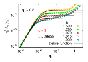
(c)Refer to captionΒ Β Β Β  (d)Refer to caption

Figure 15: Log-log plot of qβŠ₯2​SβŠ₯​(qβŠ₯)superscriptsubscriptπ‘žbottom2subscript𝑆bottomsubscriptπ‘žbottomq_{\bot}^{2}S_{\bot}(q_{\bot}) vs.Β qβŠ₯subscriptπ‘žbottomq_{\bot} in d=3𝑑3d=3 dimensions for qb=0.2subscriptπ‘žπ‘0.2q_{b}=0.2 (a), 0.1 (b), 0.03 (c) and 0.01 (d), for several choices of the force parameter b=exp⁑(f/kB​T)𝑏𝑓subscriptπ‘˜π΅π‘‡b=\exp(f/k_{B}T), as indicated. The curves are the Debye function, Eq.Β (49) with XβŠ₯=32​qβŠ₯2β€‹βŸ¨Rg,βŠ₯2⟩subscript𝑋bottom32superscriptsubscriptπ‘žbottom2delimited-⟨⟩superscriptsubscript𝑅𝑔bottom2X_{\bot}=\frac{3}{2}q_{\bot}^{2}\langle R_{g,\bot}^{2}\rangle. When the data settle down at a horizontal plateau, it yields an estimate of 4/(3β€‹βŸ¨Rg,βŠ₯2⟩)43delimited-⟨⟩superscriptsubscript𝑅𝑔bottom24/(3\langle R_{g,\bot}^{2}\rangle).

(a)Refer to captionΒ Β Β Β  (b)Refer to caption

(c)Refer to captionΒ Β Β Β  (d)Refer to caption

Figure 16: Log-log plot of qβŠ₯2​SβŠ₯​(qβŠ₯)superscriptsubscriptπ‘žbottom2subscript𝑆bottomsubscriptπ‘žbottomq_{\bot}^{2}S_{\bot}(q_{\bot}) vs.Β qβŠ₯subscriptπ‘žbottomq_{\bot} in d=2𝑑2d=2 dimensions for qb=0.2subscriptπ‘žπ‘0.2q_{b}=0.2 (a), 0.1 (b), 0.05 (c) and 0.03 (d), for several choices of the force parameter b=exp⁑(f/kB​T)𝑏𝑓subscriptπ‘˜π΅π‘‡b=\exp(f/k_{B}T), as indicated. The curves are the Debye function, Eq.Β (49) with XβŠ₯=3​qβŠ₯2β€‹βŸ¨Rg,βŠ₯2⟩subscript𝑋bottom3superscriptsubscriptπ‘žbottom2delimited-⟨⟩superscriptsubscript𝑅𝑔bottom2X_{\bot}=3q_{\bot}^{2}\langle R_{g,\bot}^{2}\rangle, and the straight line shows the excluded volume power law (slope =2βˆ’1/Ξ½absent21𝜈=2-1/\nu). From the Debye plateau 2/(3β€‹βŸ¨Rg,βŠ₯2⟩)23delimited-⟨⟩superscriptsubscript𝑅𝑔bottom22/(3\langle R_{g,\bot}^{2}\rangle) can be extracted.

VI Conclusions

In this paper we have presented a comparative simulation study of the single-chain structure factor S​(q)π‘†π‘žS(q) for variable stiffness of the macromolecules in both d=2𝑑2d=2 and d=3𝑑3d=3 dimensions, both for coils in equilibrium in dilute solution under good solvent conditions, and for polymers under the influence of a stretching force. Characteristic linear dimensions of the macromolecules that are needed in the theoretical interpretation of S​(q)π‘†π‘žS(q), have in our Monte Carlo simulation always been estimated directly and hence independently, such as the mean square gyration radius ⟨Rg2⟩delimited-⟨⟩superscriptsubscript𝑅𝑔2\langle R_{g}^{2}\rangle and the persistence length β„“psubscriptℓ𝑝\ell_{p}. In the presence of stretching forces, the extension ⟨X⟩delimited-βŸ¨βŸ©π‘‹\langle X\rangle in the direction of the force (as well as fluctuations ⟨X2βŸ©βˆ’βŸ¨X⟩2delimited-⟨⟩superscript𝑋2superscriptdelimited-βŸ¨βŸ©π‘‹2\langle X^{2}\rangle-\langle X\rangle^{2}, and components of the gyration radius ⟨RgβŠ₯2⟩delimited-⟨⟩superscriptsubscript𝑅limit-from𝑔bottom2\langle R_{g\bot}^{2}\rangle and ⟨Rg||2⟩\langle R_{g||}^{2}\rangle have been obtained as well. Of course, as usual the simulations are performed for the strictly monodisperse case, the number of bonds N𝑁N and hence also the contour length L=N​ℓb𝐿𝑁subscriptℓ𝑏L=N\ell_{b} of the chain molecules are known input parameters of the simulation. In this respect, a more definite interpretation of the outcome of the simulations can be expected, than would be expected for corresponding experiments (where polydispersity is a problem, and often the average contour length is not a priori known but must also be extracted from fitting suitable experimental data). Of course, the drawback of our Monte Carlo simulations on a lattice is the highly idealized character of such coarse-grained model as used here, the self-avoiding walk with additional energy penalty for making kinks. Nevertheless, the comparison between our simulation results for the mean square gyration radius versus the number of β€œKuhn segments” nKsubscript𝑛𝐾n_{K} with corresponding experimental data (Fig.Β 1) is very encouraging: one not only notes a striking similarity between simulation and experiment, but we stress that also the same range of dimensionless variables (nK(n_{K} and ⟨Rg2⟩/(2​ℓp)2delimited-⟨⟩superscriptsubscript𝑅𝑔2superscript2subscriptℓ𝑝2\langle R_{g}^{2}\rangle/(2\ell_{p})^{2} ) is accessible. The simulation has the bonus that directly single-chain properties are accessible (no extrapolation as a function of the concentration c𝑐c of the solution towards cβ†’0→𝑐0c\rightarrow 0 is required and by changing the energy parameter Ο΅b/kB​Tsubscriptitalic-ϡ𝑏subscriptπ‘˜π΅π‘‡\epsilon_{b}/k_{B}T, that describes the cost of making a kink along the walk, in units of the thermal energy, the stiffness is easily controlled. In experiment, stiffness can only be widely varied by combining data for polymers with different chemical structure.

From our data we have confirmed a conclusion drawn already from our previous study of mean square end-to-end distances, namely that in d=2𝑑2d=2 a direct crossover occurs from rod-like behavior to self-avoiding walks, with a scaling ⟨Rg2βŸ©βˆβ„“p1/2​L3/2proportional-todelimited-⟨⟩superscriptsubscript𝑅𝑔2superscriptsubscriptℓ𝑝12superscript𝐿32\langle R_{g}^{2}\rangle\propto\ell_{p}^{1/2}L^{3/2}, without the existence of any intermediate regime with Gaussian behavior (Fig.Β 3). In d=3𝑑3d=3, however, such an intermediate regime has been found, Fig.Β 2, for 1β‰ͺnKβ‰ͺnKβˆ—βˆ(β„“p/D)ΞΆmuch-less-than1subscript𝑛𝐾much-less-thansuperscriptsubscript𝑛𝐾proportional-tosuperscriptsubscriptβ„“π‘π·πœ1\ll n_{K}\ll n_{K}^{*}\propto(\ell_{p}/D)^{\zeta}, where D𝐷D is the local chain diameter and the exponent ΢𝜁\zeta is in the range 1.5≀΢≀21.5𝜁21.5\leq\zeta\leq 2. Thus, there is no universal value nKβˆ—superscriptsubscript𝑛𝐾n_{K}^{*} where excluded volume effects set in, but rather nKβˆ—β†’βˆžβ†’subscriptsuperscript𝑛𝐾n^{*}_{K}\rightarrow\infty for β„“p/Dβ†’βˆžβ†’subscriptℓ𝑝𝐷\ell_{p}/D\rightarrow\infty.

In the equilibrium structure factor S​(q)π‘†π‘žS(q), in the absence of stretching forces, correspondingly several regimes can be distinguished. For small enough qπ‘žq, the standard Guinier behavior always occurs, which contains the information on ⟨Rg2⟩delimited-⟨⟩superscriptsubscript𝑅𝑔2\langle R_{g}^{2}\rangle, of course. For d=2𝑑2d=2, one then always has the excluded volume regime (for long enough chains), S​(q)∝qβˆ’4/3proportional-toπ‘†π‘žsuperscriptπ‘ž43S(q)\propto q^{-4/3}, and possibly (for rather stiff chains) a crossover to rod-like behavior (S​(q)∝qβˆ’1)proportional-toπ‘†π‘žsuperscriptπ‘ž1(S(q)\propto q^{-1}) sets in gradually. A Gaussian behavior S​(q)∝qβˆ’2proportional-toπ‘†π‘žsuperscriptπ‘ž2S(q)\propto q^{-2} is never seen, unlike the case d=3𝑑3d=3, where this behavior does become visible for very stiff chains (before for still larger qπ‘žq the rod-like behavior starts). The excluded volume power law, S​(q)∝qβˆ’1/Ξ½proportional-toπ‘†π‘žsuperscriptπ‘ž1𝜈S(q)\propto q^{-1/\nu} with Ξ½β‰ˆ0.588𝜈0.588\nu\approx 0.588, is only visible for not very stiff chains (if chain lengths L≀25600𝐿25600L\leq 25600 are analyzed, as done here: if Lβ†’βˆžβ†’πΏL\rightarrow\infty, this power law would emerge for any finite value of the persistence length, of course). This pattern of behavior (Fig.Β 4), of course, could have been a priori expected, but we are also able to show via Kratky plots (qLS(q)(qLS(q) vs.Β q​Lπ‘žπΏqL) that for semiflexible chains in d=3𝑑3d=3 the expressions derived by Kholodenko and by Stepanow provide a quantitatively accurate description. It is found that for large qπ‘žq this quantity q​L​S​(q)π‘žπΏπ‘†π‘žqLS(q) settles down at Ο€πœ‹\pi, unlike the behavior predicted for flexible chains (the Debye function predicts q​L​S​(q)∝qβˆ’1proportional-toπ‘žπΏπ‘†π‘žsuperscriptπ‘ž1qLS(q)\propto q^{-1} for large qπ‘žq). However, the onset of the plateau occurs gradually in the decade 1<q​ℓp<101π‘žsubscriptℓ𝑝101<q\ell_{p}<10; thus the onset of the plateau allows an estimation of β„“psubscriptℓ𝑝\ell_{p} only somewhat roughly. The peak position of the Kratky plot (Figs.Β 5,6) reflects the theoretically expected scaling of the gyration radius with L𝐿L and β„“psubscriptℓ𝑝\ell_{p}, even though in the Kratky plot (Fig.Β 5) direct evidence for excluded volume effects seem to be minor.

Des CloizeauxΒ 18 derived from the Kratky-Porod model that for Lβ†’βˆžβ†’πΏL\rightarrow\infty one should have L​q​S​(q)=Ο€+const​(q​ℓp)βˆ’1πΏπ‘žπ‘†π‘žπœ‹constsuperscriptπ‘žsubscriptℓ𝑝1LqS(q)=\pi+\textrm{const}(q\ell_{p})^{-1}, with the constant being predicted to be 2/3 {Eq.Β (1)}. Unfortunately, this result is at variance with our numerical results (Fig.Β 7). The reason for this problem is still not clear.

Turning to the behavior of chains under the influence of stretching forces, we have shown that for weak forces, where linear response holds, excluded volume effects invalidate the Kratky-Porod model completely in d=2𝑑2d=2 dimensions, and one typically observes a broad range of forces where the extension versus force relation is a power law, and also ⟨RgβŠ₯2⟩,⟨X2βŸ©βˆ’βŸ¨X⟩2delimited-⟨⟩superscriptsubscript𝑅limit-from𝑔bottom2delimited-⟨⟩superscript𝑋2superscriptdelimited-βŸ¨βŸ©π‘‹2\langle R_{g\bot}^{2}\rangle,\langle X^{2}\rangle-\langle X\rangle^{2} are found to scale like (f​ℓp/kB​T)1/Ξ½βˆ’2superscript𝑓subscriptℓ𝑝subscriptπ‘˜π΅π‘‡1𝜈2(f\ell_{p}/k_{B}T)^{1/\nu-2} in this β€œPincus blob” regime. In d=3𝑑3d=3, dimensions, however, a Pincus blob regime also exists, but its observability also is restricted. For large kB​T/fsubscriptπ‘˜π΅π‘‡π‘“k_{B}T/f, however, the (continuum) Kratky-Porod descriptions is not valid for our discrete lattice model either: it is found that then ⟨RgβŠ₯2⟩delimited-⟨⟩superscriptsubscript𝑅limit-from𝑔bottom2\langle R_{g\bot}^{2}\rangle and ⟨X2βŸ©βˆ’βŸ¨X⟩2delimited-⟨⟩superscript𝑋2superscriptdelimited-βŸ¨βŸ©π‘‹2\langle X^{2}\rangle-\langle X\rangle^{2} decrease like exp⁑(βˆ’f/kB​T)𝑓subscriptπ‘˜π΅π‘‡\exp(-f/k_{B}T) for f/kB​T≫1much-greater-than𝑓subscriptπ‘˜π΅π‘‡1f/k_{B}T\gg 1.

Although the excluded volume effects show up rather clearly in the chain extensions and gyration radii components, it turns out that Benoit’s extension of the Debye formula to stretched chainsΒ 30 is a surprisingly accurate description of both the transverse (SβŠ₯​(qβŠ₯))subscript𝑆bottomsubscriptπ‘žbottom(S_{\bot}(q_{\bot})) and parallel parts (S||​(q||)S_{||}(q_{||})) of the structure factor. The oscillatory behavior of S||(q||S_{||}(q_{||}) for strongly stretched chains shows that their conformations resemble a string of elastically coupled particles. Thus, if measurable, the structure factor of stretched chains would add valuable details to the picture of their conformations.

As we have emphasized in our paper, the statistical mechanics of semiflexible polymers has been a longstanding and controversial problem of polymer science. The subject is of great relevance for biopolymers, but also of broad interest in material science. We expect that the present study will be useful both for the interpretation of experiments and stimulate further theoretical studies, such as of the interplay between solvent quality and chain stiffness.

Acknowledgements.
We are grateful to the Deutsche Forschungsgemeinschaft (DFG) for support under grant No SFB 625/A3, and to the John von Neumann Institute for Computing (NIC JΓΌlich) for a generous grant of computer time. We are particularly indebted to S. Stepanow for his help with the explicit calculation of his exact formula for the structure factor of the Kratky-Porod model. We are also indebted to Hyuk Yu for pointing out Ref.Β 12 to us, and to C. Pierleoni for drawing our attention to Ref.Β 34 . H.-P. Hsu thanks K. Ch. Daoulas for stimulating discussions.

Appendix A Scattering function of random walk chains under constant pulling force

The paper by Benoit et al.Β 30 uses the distribution function of the end-to-end vector of a Gaussian chain of ∣iβˆ’j∣delimited-βˆ£βˆ£π‘–π‘—\mid i-j\mid repeat units for the calculation of the single chain scattering function. The result is the well-known Debye function.

Following an idea from Doi’s bookΒ Doibook one can derive the diffusion equation yielding the end-to-end vector distribution in the following way. Assume a step-wise Markov growth of the chain

P​(Rβ†’,N)=βˆ‘iP​(Rβ†’βˆ’lβ†’i,Nβˆ’1)​p​(lβ†’i).𝑃→𝑅𝑁subscript𝑖𝑃→𝑅subscript→𝑙𝑖𝑁1𝑝subscript→𝑙𝑖P(\vec{R},N)=\sum_{i}P(\vec{R}-\vec{l}_{i},N-1)p(\vec{l}_{i})\,. (68)

The sum over β€œi” goes over an isotropic bond vector set, i.e., both lβ†’isubscript→𝑙𝑖\vec{l}_{i} and βˆ’lβ†’isubscript→𝑙𝑖-\vec{l}_{i} are members of the set.

Expanding the right side to first order in N𝑁N and to second order in R→→𝑅\vec{R} yields

P​(Rβ†’βˆ’lβ†’i,Nβˆ’1)=P​(Rβ†’,N)βˆ’βˆ‚Pβˆ‚Nβˆ’βˆ‘Ξ±=13βˆ‚Pβˆ‚Rα​li,Ξ±+12β€‹βˆ‘Ξ±=13βˆ‘Ξ²=13βˆ‚2Pβˆ‚RΞ±β€‹βˆ‚Rβ​li,α​li,Ξ²+….𝑃→𝑅subscript→𝑙𝑖𝑁1𝑃→𝑅𝑁𝑃𝑁superscriptsubscript𝛼13𝑃subscript𝑅𝛼subscript𝑙𝑖𝛼12superscriptsubscript𝛼13superscriptsubscript𝛽13superscript2𝑃subscript𝑅𝛼subscript𝑅𝛽subscript𝑙𝑖𝛼subscript𝑙𝑖𝛽…P(\vec{R}-\vec{l}_{i},N-1)=P(\vec{R},N)-\frac{\partial P}{\partial N}-\sum_{\alpha=1}^{3}\frac{\partial P}{\partial R_{\alpha}}l_{i,\alpha}+\frac{1}{2}\sum_{\alpha=1}^{3}\sum_{\beta=1}^{3}\frac{\partial^{2}P}{\partial R_{\alpha}\partial R_{\beta}}l_{i,\alpha}l_{i,\beta}+\ldots\,. (69)

Averaging the derivatives with respect to RΞ±subscript𝑅𝛼R_{\alpha} with a symmetric bond probability p​(lβ†’i)𝑝subscript→𝑙𝑖p(\vec{l}_{i}) (in the simplest case this is just one over the number of bonds) gives zero for the first derivative and δα​β​l2/3subscript𝛿𝛼𝛽superscript𝑙23\delta_{\alpha\beta}l^{2}/3 for the second term, resulting in the diffusion equation

βˆ‚Pβˆ‚N=l26β€‹βˆ‡2P𝑃𝑁superscript𝑙26superscriptβˆ‡2𝑃\frac{\partial P}{\partial N}=\frac{l^{2}}{6}\nabla^{2}P (70)

Solving this for a bulk chain gives the well known result for the end-to-end vector distribution

P​(Rβ†’,N)=(2​π​N​l2/3)βˆ’3/2​exp⁑(βˆ’3​R22​N​l2),𝑃→𝑅𝑁superscript2πœ‹π‘superscript𝑙23323superscript𝑅22𝑁superscript𝑙2P(\vec{R},N)=(2\pi Nl^{2}/3)^{-3/2}\exp\left(-\frac{3R^{2}}{2Nl^{2}}\right)\,, (71)

The Debye function can than be derived by averaging with this probability, as is done in the Benoit et al. paper.

The derivation above is useful as a starting point for a calculation of the scattering function for a chain that is pulled. In this case the bond probabilities are not symmetric. For our model we have

p0subscript𝑝0\displaystyle p_{0} =\displaystyle= bb2+4​b+1𝑏superscript𝑏24𝑏1\displaystyle\frac{b}{b^{2}+4b+1} (72)
p+subscript𝑝\displaystyle p_{+} =\displaystyle= b2b2+4​b+1superscript𝑏2superscript𝑏24𝑏1\displaystyle\frac{b^{2}}{b^{2}+4b+1}
pβˆ’subscript𝑝\displaystyle p_{-} =\displaystyle= 1b2+4​b+11superscript𝑏24𝑏1\displaystyle\frac{1}{b^{2}+4b+1} (73)

for moves perpendicular to the pulling direction, in +X𝑋+X direction and in βˆ’X𝑋-X direction, respectively, where b=exp⁑(f​l/kB​T)𝑏𝑓𝑙subscriptπ‘˜π΅π‘‡b=\exp(fl/k_{B}T) with l=1𝑙1l=1 is used as in the main text. When we now perform the expansion of Eq.Β (69) and perform the average over the bond probabilities we obtain

βˆ‚Pβˆ‚N=βˆ’(p+βˆ’pβˆ’)​lβ€‹βˆ‚Pβˆ‚X+p0​l2​(βˆ‚2Pβˆ‚Y2+βˆ‚2Pβˆ‚Z2)+p++pβˆ’2​l2β€‹βˆ‚2Pβˆ‚X2𝑃𝑁subscript𝑝subscript𝑝𝑙𝑃𝑋subscript𝑝0superscript𝑙2superscript2𝑃superscriptπ‘Œ2superscript2𝑃superscript𝑍2subscript𝑝subscript𝑝2superscript𝑙2superscript2𝑃superscript𝑋2\frac{\partial P}{\partial N}=-(p_{+}-p_{-})l\frac{\partial P}{\partial X}+p_{0}l^{2}\left(\frac{\partial^{2}P}{\partial Y^{2}}+\frac{\partial^{2}P}{\partial Z^{2}}\right)+\frac{p_{+}+p_{-}}{2}l^{2}\frac{\partial^{2}P}{\partial X^{2}} (74)

For p+=pβˆ’=p0subscript𝑝subscript𝑝subscript𝑝0p_{+}=p_{-}=p_{0} this reduces to the normal diffusion equation. This equation has to be solved with the boundary conditions

P​(Rβ†’,0)𝑃→𝑅0\displaystyle P(\vec{R},0) =\displaystyle= δ​(Rβ†’)𝛿→𝑅\displaystyle\delta(\vec{R}) (75)
P​(Rβ†’,N)𝑃→𝑅𝑁\displaystyle P(\vec{R},N) β†’β†’\displaystyle\rightarrow 0forRβ†’βˆžβ†’0for𝑅\displaystyle 0\qquad{\rm for}\qquad R\rightarrow\infty

Let us define DβŠ₯=2​p0​l2subscript𝐷bottom2subscript𝑝0superscript𝑙2D_{\bot}=2p_{0}l^{2}, D||=(p++pβˆ’)​l2D_{||}=(p_{+}+p_{-})l^{2}, and v=(p+βˆ’pβˆ’)​l𝑣subscript𝑝subscript𝑝𝑙v=(p_{+}-p_{-})l, so we have

βˆ‚Pβˆ‚N=βˆ’vβ€‹βˆ‚Pβˆ‚X+12​DβŠ₯​(βˆ‚2Pβˆ‚Y2+βˆ‚2Pβˆ‚Z2)+12​D||β€‹βˆ‚2Pβˆ‚X2.\frac{\partial P}{\partial N}=-v\frac{\partial P}{\partial X}+\frac{1}{2}D_{\bot}\left(\frac{\partial^{2}P}{\partial Y^{2}}+\frac{\partial^{2}P}{\partial Z^{2}}\right)+\frac{1}{2}D_{||}\frac{\partial^{2}P}{\partial X^{2}}\,. (76)

These are three diffusion processes in the three Cartesian directions, X𝑋X is parallel to the force, Yπ‘ŒY and Z𝑍Z are perpendicular. The solutions for the perpendicular directions are the same as for the force-free case. For the parallel direction we have an altered diffusion coefficient and a drift part to the process, i.e., a Gaussian diffusion around a deterministic drift. The complete solution to Eq.Β (76) is therefore given by

P​(X,Y,Z,N)=12​π​N​DβŠ₯​12​π​N​D||​eβˆ’Y2+Z22​N​DβŠ₯​eβˆ’(xβˆ’v​N)22​N​D||.P(X,Y,Z,N)=\frac{1}{2\pi ND_{\bot}}\frac{1}{\sqrt{2\pi ND_{||}}}e^{-\frac{Y^{2}+Z^{2}}{2ND_{\bot}}}e^{-\frac{(x-vN)^{2}}{2ND_{||}}}\,. (77)

For p0=p+=pβˆ’=1/6subscript𝑝0subscript𝑝subscript𝑝16p_{0}=p_{+}=p_{-}=1/6 we obtain back the force free solution. To calculate the scattering function we follow the procedure employed in the calculation of the Debye function in the force free case.

S​(qβ†’)=1N2β€‹βˆ‘i,j⟨ei​qβ†’β‹…rβ†’i​jβŸ©π‘†β†’π‘ž1superscript𝑁2subscript𝑖𝑗delimited-⟨⟩superscriptπ‘’β‹…π‘–β†’π‘žsubscriptβ†’π‘Ÿπ‘–π‘—S(\vec{q})=\frac{1}{N^{2}}\sum_{i,j}\langle e^{i\vec{q}\cdot\vec{r}_{ij}}\rangle (78)

can be calculated when we assume a continuous chain model (i.e. only look at distances much larger than the lattice constant) so that the distribution for the rβ†’i​jsubscriptβ†’π‘Ÿπ‘–π‘—\vec{r}_{ij} is given by the Gaussian distribution we just calculated.

S​(qβ†’)=1N2β€‹βˆ‘i,j∫d3​rβ†’i​j​P​(rβ†’i​j,∣iβˆ’j∣)​ei​qβ†’β‹…rβ†’i​jπ‘†β†’π‘ž1superscript𝑁2subscript𝑖𝑗superscript𝑑3subscriptβ†’π‘Ÿπ‘–π‘—π‘ƒsubscriptβ†’π‘Ÿπ‘–π‘—delimited-βˆ£βˆ£π‘–π‘—superscriptπ‘’β‹…π‘–β†’π‘žsubscriptβ†’π‘Ÿπ‘–π‘—S(\vec{q})=\frac{1}{N^{2}}\sum_{i,j}\int d^{3}\vec{r}_{ij}P(\vec{r}_{ij},\mid i-j\mid)e^{i\vec{q}\cdot\vec{r}_{ij}} (79)

where we have P​(rβ†’i​j,∣iβˆ’j∣)=PY​(Y,∣iβˆ’j∣)​PZ​(Z,∣iβˆ’j∣)​PX​(X,∣iβˆ’j∣)𝑃subscriptβ†’π‘Ÿπ‘–π‘—delimited-βˆ£βˆ£π‘–π‘—subscriptπ‘ƒπ‘Œπ‘Œdelimited-βˆ£βˆ£π‘–π‘—subscript𝑃𝑍𝑍delimited-βˆ£βˆ£π‘–π‘—subscript𝑃𝑋𝑋delimited-βˆ£βˆ£π‘–π‘—P(\vec{r}_{ij},\mid i-j\mid)=P_{Y}(Y,\mid i-j\mid)P_{Z}(Z,\mid i-j\mid)P_{X}(X,\mid i-j\mid) and PYsubscriptπ‘ƒπ‘ŒP_{Y} and PZsubscript𝑃𝑍P_{Z} have the same functional form and all Pisubscript𝑃𝑖P_{i} are normalized to one individually.

Scattering in the perpendicular direction

S​(qβ†’βŠ₯)=1N2𝑆subscriptβ†’π‘žbottom1superscript𝑁2\displaystyle S(\vec{q}_{\bot})=\frac{1}{N^{2}} βˆ‘i,jβˆ«π‘‘Yβ€‹βˆ«π‘‘Zsubscript𝑖𝑗differential-dπ‘Œdifferential-d𝑍\displaystyle\sum_{i,j}\int dY\int dZ
PY​(Y,∣iβˆ’j∣)​PZ​(Z,∣iβˆ’j∣)​ei​qβ†’βŠ₯⋅ρ→i​jsubscriptπ‘ƒπ‘Œπ‘Œdelimited-βˆ£βˆ£π‘–π‘—subscript𝑃𝑍𝑍delimited-βˆ£βˆ£π‘–π‘—superscript𝑒⋅𝑖subscriptβ†’π‘žbottomsubscriptβ†’πœŒπ‘–π‘—\displaystyle P_{Y}(Y,\mid i-j\mid)P_{Z}(Z,\mid i-j\mid)e^{i\vec{q}_{\bot}\cdot\vec{\rho}_{ij}}

where ρi​j=Y​e^Y+Z​e^ZsubscriptπœŒπ‘–π‘—π‘Œsubscript^π‘’π‘Œπ‘subscript^𝑒𝑍\rho_{ij}=Y\hat{e}_{Y}+Z\hat{e}_{Z}. So we have to evaluate

S​(qY,qZ)𝑆subscriptπ‘žπ‘Œsubscriptπ‘žπ‘\displaystyle S(q_{{}_{Y}},q_{{}_{Z}})
=1N2β€‹βˆ‘i,jβˆ«π‘‘Y​12β€‹Ο€β€‹βˆ£iβˆ’jβˆ£β€‹DβŠ₯​eβˆ’Y22β€‹βˆ£iβˆ’jβˆ£β€‹DβŠ₯​ei​qY​Yabsent1superscript𝑁2subscript𝑖𝑗differential-dπ‘Œ12πœ‹delimited-βˆ£βˆ£π‘–π‘—subscript𝐷bottomsuperscript𝑒superscriptπ‘Œ22delimited-βˆ£βˆ£π‘–π‘—subscript𝐷bottomsuperscript𝑒𝑖subscriptπ‘žπ‘Œπ‘Œ\displaystyle=\frac{1}{N^{2}}\sum_{i,j}\int dY\frac{1}{\sqrt{2\pi\mid i-j\mid D_{\bot}}}e^{-\frac{Y^{2}}{2\mid i-j\mid D_{\bot}}}e^{iq_{{}_{Y}}Y}
βˆ«π‘‘Z​12β€‹Ο€β€‹βˆ£iβˆ’jβˆ£β€‹DβŠ₯​eβˆ’Z22β€‹βˆ£iβˆ’jβˆ£β€‹DβŠ₯​ei​qZ​Zdifferential-d𝑍12πœ‹delimited-βˆ£βˆ£π‘–π‘—subscript𝐷bottomsuperscript𝑒superscript𝑍22delimited-βˆ£βˆ£π‘–π‘—subscript𝐷bottomsuperscript𝑒𝑖subscriptπ‘žπ‘π‘\displaystyle\int dZ\frac{1}{\sqrt{2\pi\mid i-j\mid D_{\bot}}}e^{-\frac{Z^{2}}{2\mid i-j\mid D_{\bot}}}e^{iq_{{}_{Z}}Z} (81)

resulting in

S​(qβŠ₯)=1N2β€‹βˆ‘i,jeβˆ’qβŠ₯2​DβŠ₯β€‹βˆ£iβˆ’j∣2𝑆subscriptπ‘žbottom1superscript𝑁2subscript𝑖𝑗superscript𝑒subscriptsuperscriptπ‘ž2bottomsubscript𝐷bottomdelimited-βˆ£βˆ£π‘–π‘—2S(q_{\bot})=\frac{1}{N^{2}}\sum_{i,j}e^{-\frac{q^{2}_{\bot}D_{\bot}\mid i-j\mid}{2}} (82)

This is evaluated by a continuum approximation for the two sums, βˆ‘iβ†’βˆ«0N𝑑uβ†’subscript𝑖superscriptsubscript0𝑁differential-d𝑒\sum_{i}\rightarrow\int_{0}^{N}du and βˆ‘jβ†’βˆ«0N𝑑vβ†’subscript𝑗superscriptsubscript0𝑁differential-d𝑣\sum_{j}\rightarrow\int_{0}^{N}dv which finally yields:

S​(qβŠ₯)=4N​qβŠ₯2​DβŠ₯+8N2​qβŠ₯4​DβŠ₯2​(eβˆ’qβŠ₯2​DβŠ₯​N2βˆ’1).𝑆subscriptπ‘žbottom4𝑁superscriptsubscriptπ‘žbottom2subscript𝐷bottom8superscript𝑁2superscriptsubscriptπ‘žbottom4superscriptsubscript𝐷bottom2superscript𝑒superscriptsubscriptπ‘žbottom2subscript𝐷bottom𝑁21S(q_{\bot})=\frac{4}{Nq_{\bot}^{2}D_{\bot}}+\frac{8}{N^{2}q_{\bot}^{4}D_{\bot}^{2}}\left(e^{-\frac{q_{\bot}^{2}D_{\bot}N}{2}}-1\right)\,. (83)

Scattering in the parallel direction

S​(q||)=1N2β€‹βˆ‘i,jβˆ«π‘‘X​12β€‹Ο€β€‹βˆ£iβˆ’jβˆ£β€‹D||​eβˆ’(xβˆ’vβ€‹βˆ£iβˆ’j∣)22β€‹βˆ£iβˆ’jβˆ£β€‹D||​ei​q||​XS(q_{||})=\frac{1}{N^{2}}\sum_{i,j}\int dX\frac{1}{\sqrt{2\pi\mid i-j\mid D_{||}}}e^{-\frac{(x-v\mid i-j\mid)^{2}}{2\mid i-j\mid D_{||}}}e^{iq_{||}X} (84)

which now results in

S​(q||)=1N2β€‹βˆ‘i,jeβˆ’q||​D||β€‹βˆ£iβˆ’j∣2​cos⁑(q||​vβ€‹βˆ£iβˆ’j∣).S(q_{||})=\frac{1}{N^{2}}\sum_{i,j}e^{-\frac{q_{||}D_{||}\mid i-j\mid}{2}}\cos(q_{||}v\mid i-j\mid)\,. (85)

Performing the final calculation again in the continuum approximation gives

S​(q||)\displaystyle S(q_{||})
=4N​D||​q||2q||4​D||2+4​v2​q||2\displaystyle=\frac{4}{N}\frac{D_{||}q_{||}^{2}}{q_{||}^{4}D_{||}^{2}+4v^{2}q_{||}^{2}}
+8N2​q||4​D||2βˆ’4​v2​q||2(q||4​D||2+4​v2​q||2)2​(eβˆ’q||2​D||​N2​cos⁑(N​v​q||)βˆ’1)\displaystyle+\frac{8}{N^{2}}\frac{q^{4}_{||}D^{2}_{||}-4v^{2}q_{||}^{2}}{(q^{4}_{||}D_{||}^{2}+4v^{2}q_{||}^{2})^{2}}\left(e^{-\frac{q_{||}^{2}D_{||}N}{2}}\cos(Nvq_{||})-1\right)
βˆ’32N2​q||3​D||​v(q||4​D||2+4​v2​q||2)2​eβˆ’q||2​D||​N2​sin⁑(N​v​q||)\displaystyle-\frac{32}{N^{2}}\frac{q_{||}^{3}D_{||}v}{(q^{4}_{||}D^{2}_{||}+4v^{2}q_{||}^{2})^{2}}e^{-\frac{q_{||}^{2}D_{||}N}{2}}\sin(Nvq_{||}) (86)

This result determines our scattering functions with parameters depending on the applied force f𝑓f, so these equations contain no free parameters. Note that both functions reduce to the Debye function for the force free isotropic case (v=0𝑣0v=0, DβŠ₯=D||=l2/3D_{\bot}=D_{||}=l^{2}/3) as it should be, because the scattering function does not depend on the direction of the scattering vector in this case.

For fitting purposes it might yield better results to replace some of the quantities by average values determined in the simulation. For the Yπ‘ŒY and the Z𝑍Z components simple Gaussian statistics holds

⟨Y⟩delimited-βŸ¨βŸ©π‘Œ\displaystyle\langle Y\rangle =\displaystyle= ⟨Z⟩=0delimited-βŸ¨βŸ©π‘0\displaystyle\langle Z\rangle=0 (87)
⟨Y2⟩delimited-⟨⟩superscriptπ‘Œ2\displaystyle\langle Y^{2}\rangle =\displaystyle= ⟨Z2⟩=N​DβŠ₯delimited-⟨⟩superscript𝑍2𝑁subscript𝐷bottom\displaystyle\langle Z^{2}\rangle=ND_{\bot} (88)
⟨Rg,Y2⟩delimited-⟨⟩superscriptsubscriptπ‘…π‘”π‘Œ2\displaystyle\langle R_{g,Y}^{2}\rangle =\displaystyle= ⟨Rg,Z2⟩=N​DβŠ₯6delimited-⟨⟩subscriptsuperscript𝑅2𝑔𝑍𝑁subscript𝐷bottom6\displaystyle\langle R^{2}_{g,Z}\rangle=\frac{ND_{\bot}}{6} (89)

but in the force direction we can calculate from Eq.Β (77) for the moments of the end-to-end distance

⟨X⟩delimited-βŸ¨βŸ©π‘‹\displaystyle\langle X\rangle =\displaystyle= N​v𝑁𝑣\displaystyle Nv (90)
⟨X2⟩delimited-⟨⟩superscript𝑋2\displaystyle\langle X^{2}\rangle =\displaystyle= N2​v2+N​D||\displaystyle N^{2}v^{2}+ND_{||} (91)
βŸ¨Ξ”β€‹X2⟩delimited-βŸ¨βŸ©Ξ”superscript𝑋2\displaystyle\langle\Delta X^{2}\rangle =\displaystyle= N​D||\displaystyle ND_{||} (92)
⟨Rg,X2⟩delimited-⟨⟩subscriptsuperscript𝑅2𝑔𝑋\displaystyle\langle R^{2}_{g,X}\rangle =\displaystyle= N​D||6+D||​N2​v212.\displaystyle\frac{ND_{||}}{6}+\frac{D_{||}N^{2}v^{2}}{12}\,. (93)

When we now rewrite the scattering functions in terms of moments of the end-to-end vector or gyration tensor, we obtain

S​(qβŠ₯)𝑆subscriptπ‘žbottom\displaystyle S(q_{\bot}) (94)
=43​qβŠ₯2β€‹βŸ¨Rg,βŠ₯2⟩+8[3​qβŠ₯2β€‹βŸ¨Rg,βŠ₯2⟩]2​(eβˆ’3​qβŠ₯2β€‹βŸ¨Rg,βŠ₯2⟩2βˆ’1).absent43superscriptsubscriptπ‘žbottom2delimited-⟨⟩subscriptsuperscript𝑅2𝑔bottom8superscriptdelimited-[]3superscriptsubscriptπ‘žbottom2delimited-⟨⟩subscriptsuperscript𝑅2𝑔bottom2superscript𝑒3superscriptsubscriptπ‘žbottom2delimited-⟨⟩subscriptsuperscript𝑅2𝑔bottom21\displaystyle=\frac{4}{3q_{\bot}^{2}\langle R^{2}_{g,\bot}\rangle}+\frac{8}{\left[3q_{\bot}^{2}\langle R^{2}_{g,\bot}\rangle\right]^{2}}\left(e^{-\frac{3q_{\bot}^{2}\langle R^{2}_{g,\bot}\rangle}{2}}-1\right)\,.

This is the Debye function with the appropriate prefactors, because for ⟨Rg,βŠ₯2⟩=2/3β€‹βŸ¨Rg2⟩delimited-⟨⟩subscriptsuperscript𝑅2𝑔bottom23delimited-⟨⟩superscriptsubscript𝑅𝑔2\langle R^{2}_{g,\bot}\rangle=2/3\langle R_{g}^{2}\rangle it reduces to the standard function, Eq.Β (22). For the scattering parallel to the pulling direction we can write

S​(q||)\displaystyle S(q_{||}) (95)
=4​q||β€‹βŸ¨Ξ”β€‹X2⟩q||4β€‹βŸ¨Ξ”β€‹X2⟩2+4​q||2β€‹βŸ¨X⟩2\displaystyle=4\frac{q_{||}\langle\Delta X^{2}\rangle}{q_{||}^{4}\langle\Delta X^{2}\rangle^{2}+4q_{||}^{2}\langle X\rangle^{2}}
+8​q||4β€‹βŸ¨Ξ”β€‹X2⟩2βˆ’4​q||2β€‹βŸ¨X⟩2(q||4β€‹βŸ¨Ξ”β€‹X2⟩2+4​q||2β€‹βŸ¨X⟩2)2​(eβˆ’q||2β€‹βŸ¨Ξ”β€‹X2⟩2​cos⁑(q||β€‹βŸ¨X⟩)βˆ’1)\displaystyle+8\frac{q_{||}^{4}\langle\Delta X^{2}\rangle^{2}-4q_{||}^{2}\langle X\rangle^{2}}{(q_{||}^{4}\langle\Delta X^{2}\rangle^{2}+4q^{2}_{||}\langle X\rangle^{2})^{2}}\left(e^{-\frac{q_{||}^{2}\langle\Delta X^{2}\rangle}{2}}\cos(q_{||}\langle X\rangle)-1\right)
βˆ’32​q||3β€‹βŸ¨Ξ”β€‹X2βŸ©β€‹βŸ¨X⟩(q||4β€‹βŸ¨Ξ”β€‹X2⟩2+4​q||2β€‹βŸ¨X⟩2)2​eβˆ’q||2β€‹βŸ¨Ξ”β€‹X2⟩2​sin⁑(q||β€‹βŸ¨X⟩).\displaystyle-32\frac{q^{3}_{||}\langle\Delta X^{2}\rangle\langle X\rangle}{(q_{||}^{4}\langle\Delta X^{2}\rangle^{2}+4q_{||}^{2}\langle X\rangle^{2})^{2}}e^{-\frac{q_{||}^{2}\langle\Delta X^{2}\rangle}{2}}\sin(q_{||}\langle X\rangle)\,.

This gives the same formula as Eq.Β (65) when X||X_{||} in Eq.Β (48) is written by X||=a+i​cX_{||}=a+ic with a=q||2β€‹βŸ¨Ξ”β€‹X2⟩/2a=q_{||}^{2}\langle\Delta X^{2}\rangle/2, and c=q||β€‹βŸ¨X⟩c=q_{||}\langle X\rangle. For ⟨X⟩=0delimited-βŸ¨βŸ©π‘‹0\langle X\rangle=0 and βŸ¨Ξ”β€‹X2⟩=⟨X2⟩=6β€‹βŸ¨Rg,X2⟩=2β€‹βŸ¨Rg2⟩delimited-βŸ¨βŸ©Ξ”superscript𝑋2delimited-⟨⟩superscript𝑋26delimited-⟨⟩superscriptsubscript𝑅𝑔𝑋22delimited-⟨⟩superscriptsubscript𝑅𝑔2\langle\Delta X^{2}\rangle=\langle X^{2}\rangle=6\langle R_{g,X}^{2}\rangle=2\langle R_{g}^{2}\rangle this again reduces to the Debye function, Eq.Β (22).

Scattering in d=2𝑑2d=2

Both scattering functions as calculated in Eqs.Β (83) and (A) remain formally unchanged. However, the probabilities for the single steps change to

p0subscript𝑝0\displaystyle p_{0} =\displaystyle= bb2+2​b+1𝑏superscript𝑏22𝑏1\displaystyle\frac{b}{b^{2}+2b+1}
p+subscript𝑝\displaystyle p_{+} =\displaystyle= b2b2+2​b+1superscript𝑏2superscript𝑏22𝑏1\displaystyle\frac{b^{2}}{b^{2}+2b+1} (96)
pβˆ’subscript𝑝\displaystyle p_{-} =\displaystyle= 1b2+2​b+11superscript𝑏22𝑏1\displaystyle\frac{1}{b^{2}+2b+1}

The parallel and perpendicular diffusion coefficients as well as the drift velocity still have the same functional dependence on these probabilities. However, introducing the chain extensions into Eqs.Β (83) and (A) for d=2𝑑2d=2 changes the prediction Eq.Β (A) for the perpendicular scattering to

S​(qβŠ₯)𝑆subscriptπ‘žbottom\displaystyle S(q_{\bot})
=23​qβŠ₯2β€‹βŸ¨Rg,βŠ₯2⟩+2(3​qβŠ₯2β€‹βŸ¨Rg,βŠ₯2⟩)2​(eβˆ’3​qβŠ₯2β€‹βŸ¨Rg,βŠ₯2βŸ©βˆ’1),absent23superscriptsubscriptπ‘žbottom2delimited-⟨⟩superscriptsubscript𝑅𝑔bottom22superscript3superscriptsubscriptπ‘žbottom2delimited-⟨⟩subscriptsuperscript𝑅2𝑔bottom2superscript𝑒3superscriptsubscriptπ‘žbottom2delimited-⟨⟩subscriptsuperscript𝑅2𝑔bottom1\displaystyle=\frac{2}{3q_{\bot}^{2}\langle R_{g,\bot}^{2}\rangle}+\frac{2}{(3q_{\bot}^{2}\langle R^{2}_{g,\bot}\rangle)^{2}}\left(e^{-3q_{\bot}^{2}\langle R^{2}_{g,\bot}\rangle}-1\right)\,,

whereas it leaves Eq.Β (95) unchanged. Taking XβŠ₯=3​qβŠ₯2β€‹βŸ¨Rg,βŠ₯2⟩subscript𝑋bottom3superscriptsubscriptπ‘žbottom2delimited-⟨⟩subscriptsuperscript𝑅2𝑔bottomX_{\bot}=3q_{\bot}^{2}\langle R^{2}_{g,\bot}\rangle, the expression of Eq.Β (A) has the same formula as Eq.Β (49).

References

  • (1) P. G. de Gennes, Scaling Concepts in Polymer Physics (Cornell University Press, Ithaca, NY, 1979).
  • (2) J. Des Cloizeaux and G. Jannink, Polymers in Solution: Their Modeling and Structure (Clarendon Press, Oxford, UK, 1990).
  • (3) L. SchΓ€fer, Excluded Volume Effects in Polymer Solutions as Explained by the Renormalization Group (Springer, Berlin, 1999).
  • (4) J. S. Higgins and H. C. Benoit, Polymers and Neutron Scattering (Clarendon Press, Oxford, 1994).
  • (5) P. J. Flory, Principles of Polymer Chemistry (Cornell University Press, NY, 1953).
  • (6) M. Rubinstein and R. H. Colby, Polymer Physics (Oxford Universit Press, Oxford, UK, 2003).
  • (7) J. P. Cotton, D. Decker, H. Benoit, B. Farnoux, J. Higgins, G. Jannink, R. Ober, C. Picot, and J. des Cloizeaux, Macromolecules 7, 863 (1974).
  • (8) B. Farnoux, F. Boue, J. P. Cotton, M. Daoud, G. Jannink, M. Nierlich, and P. G. de Gennes, J. Phys. 39, 77 (1978).
  • (9) J. C. Le Guillou and J. Zinn-Justin, Phys. Rev. B 21, 3976 (1980).
  • (10) H.-P. Hsu, W. Paul and K. Binder, Macromolecules 43, 3094 (2010).
  • (11) H.-P. Hsu, W. Paul and K. Binder, Europhys. Lett. 92, 28003 (2010).
  • (12) T. Norisuye and H. Fujita, Polymer J. 14, 143 (1982).
  • (13) H.-P. Hsu and K. Binder, J. Chem. Phys. 136, 024901 (2012).
  • (14) O. Kratky and G. Porod, J. Colloid Sci. 4, 35 (1949).
  • (15) D. W. Schaefer, J. F. Joanny, and P. Pincus, Macromolecules 13, 1280 (1980).
  • (16) R. R. Netz and D. Andelman, Phys. Rep. 380, 1 (2003).
  • (17) H. Yamakawa and W. H. Stockmayer, J. Chem. Phys. 57, 2843 (1972).
  • (18) H. Yamakawa and J. Shimada, J. Chem. Phys. 83, 2607 (1985).
  • (19) J. Shimada and H. Yamakawa, J. Chem. Phys. 85, 591 (1986).
  • (20) H. Fujita, Macromolecules 21, 179 (1988).
  • (21) A. Tsuboi, T. Norisuye, and A. Teramoto, Macromolecules 29, 3597 (1996).
  • (22) H. P. Hsu, W. Paul and K. Binder, Europhys. Lett. 95 68004 (2011).
  • (23) J. des Cloizeaux, Macromolecules 6, 403 (1973).
  • (24) G. Porod, Z. Naturforschung 4a, 401 (1949).
  • (25) G. Porod, J. Polym. Sci. 10, 157 (1953).
  • (26) A. Peterlin, J. Polym. Sci. 47, 403 (1960).
  • (27) W. R. Krigbaum and S. Sasaki, J. Polym. Sci.: Polym. Phys. Ed. 19, 1339 (1981).
  • (28) M. G. Bawendi and K. F. Freed, J. Chem. Phys. 83, 2491 (1985).
  • (29) M. Rawiso, R. Duplessix and C. Picot, Macromolecules 20, 630 (1987).
  • (30) A. L. Kholodenko, Ann. Phys. 202, 186 (1990).
  • (31) A. L. Kholodenko, J. Chem. Phys. 96, 700 (1992).
  • (32) A. L. Kholodenko, Macromolecules 26, 4179 (1993).
  • (33) A. J. Spakowitz and Z.-G. Wang, Macromolecules 37, 5814 (2004).
  • (34) S. Stepanow, Eur. Phys. J. B 39, 499 (2004).
  • (35) S. Stepanow, J. Phys.: Condens. Matter 17, S1799 (2005).
  • (36) J. S. Pedersen, M. Laso and P. Schurtenberger, Phys. Rev. E 54, R5917 (1996).
  • (37) J. S. Pedersen and P. Schurtenberger, Macromolecules 29, 7602 (1996).
  • (38) J. S. Pedersen and P. Schurtenberger, Europhys. Lett. 45, 666 (1999).
  • (39) D. PΓΆtschke, P. Hickl, M. Ballauff, P.-O. Astrand, and J. S. Pedersen, Macromol. Theory Simul. 9, 345 (2000).
  • (40) H. Benoit, R. Duplessix, R. Ober, M. Daoud, J. P. Cotton, B. Farnoux, and G. Jannink, Macromolecules 8, 451 (1975).
  • (41) P. Pincus, Macromolecules 9, 386 (1976).
  • (42) S. B. Smith, L. Finzi, and C. Bustamante, Science 258, 1122 (1992).
  • (43) J. F. Marko and E. D. Siggia, Macromolecules 28, 8759 (1995).
  • (44) C. Pierleoni, G. Arialdi, and J.-P. Ryckaert, Phys. Rev. Lett. 79, 2990 (1997).
  • (45) R. R. Netz, Macromolecules 34, 7522 (2001).
  • (46) M.-N. Dessinges, B. Maier, Y. Zhang, M. Peliti, D. Bensimon, and V. Croquette, Phys. Rev. Lett. 89, 248102 (2002).
  • (47) L. Livadaru, R. R. Netz, and H. J. Kreuzer, Macromolecules 36, 3732 (2003).
  • (48) T. Hugel, M. Rief, M. Seitz, H. E. Gaub, and R. R. Netz, Phys. Rev. Lett. 94, 048301 (2005).
  • (49) Y. Seol, G. M. Skinner, and K. Visscher, Phys. Rev. Lett. 93, 118102 (2004).
  • (50) A. Prasad, Y. Hori, and J. Kondev, Phys. Rev. E 72, 041918 (2005).
  • (51) G. Morrison, C. Hyeon, N. M. Toan, B.-Y. Ha, and D. Thirumalai, Macromolecules 40, 7343 (2007).
  • (52) O. A. Saleh, D. B. McIntosh, P. Pincus and N. Ribeck, Phys. Rev. Lett. 102, 068301 (2009).
  • (53) D. B. McIntosh, N. Ribeck and O. A. Saleh, Phys. Rev. E 80, 041803 (2009).
  • (54) N. M. Toan and D. Thirumalai, Macromolecules 43, 4394 (2010).
  • (55) A. Dittmore, D. B. McIntosh, S. Halliday, and O. A. Saleh, Phys. Rev. Lett. 107, 148301 (2011).
  • (56) A. Onuki, J. Phys. Soc. Japan 54, 3656 (1985).
  • (57) P. Lindner and R. OberthΓΌr, Physica B 156 & 157, 410 (1989).
  • (58) C. Pierleoni and J.-P. Ryckaert, Macromolecules 28, 5097 (1995).
  • (59) T. Q. Nguyen and H.-H. Kausch (eds.) Flexible Polymer Chains in Elongational Flow (Springer, Berlin, 1999).
  • (60) W. Reisner, K. J. Morton, R. Riehn, Y. M. Wang, Z. Yu, M. Rosen, J. C. Sturm, S. Y. Chou, E. Frey, and R. H. Austin, Phys. Rev. Lett. 94, 196101 (2005).
  • (61) P. Cifra, J. Chem. Phys. 131, 224903 (2009).
  • (62) F. ThΓΌroff, B. Obermayer, and E. Frey, Phys. Rev. E 83, 021802 (2011).
  • (63) A. Yu. Grosberg and A. R. Khokhlov, Statistical Physics of Macromolecules (AIP Press, New York, 1994).
  • (64) J. P. Wittmer, H. Meyer, J. Baschnagel, A. Johner, S. Obukhov, L. Mattioni, M. MΓΌller and A. N. Semenov, Phys. Rev. Lett. 93, 147801 (2004).
  • (65) J. P. Wittmer, P. Beckrich, H. Meyer, A. Cavallo, A. Johner, and J. Baschnagel, Phys. Rev. E76, 011803 (2007).
  • (66) D. Shirvanyants, S. Panyukov, Q. Liao, and M. Rubinstein, Macromolecules 41, 1475 (2008).
  • (67) L. SchΓ€fer, A. Ostendorf, and J. Hager, J. Phys. A: Math. Gen. 32, 7875 (1999).
  • (68) H. Benoit and P. Doty, J. Phys. Chem. 57, 958 (1953).
  • (69) T. Neugebauer, Ann. Phys. 434, 509 (1943).
  • (70) H.-P. Hsu, W. Paul, and K. Binder, J. Chem. Phys. 129, 204904 (2008).
  • (71) S. Stepanow (private communication).
  • (72) V. J. Emery and J. D. Axe, Phys. Rev. Lett. 40, 1507 (1978).
  • (73) A. Ricci, P. Nielaba, S. Sengupta, and K. Binder, Phys. Rev. E 75, 011405 (2007).
  • (74) M. Doi and s. F. Edwards, The Theory of Polymer Dynamics (Clarendon Press, Oxford, 1986).