Power-law distributions in binned empirical data

Abstract

Many man-made and natural phenomena, including the intensity of earthquakes, population of cities and size of international wars, are believed to follow power-law distributions. The accurate identification of power-law patterns has significant consequences for correctly understanding and modeling complex systems. However, statistical evidence for or against the power-law hypothesis is complicated by large fluctuations in the empirical distribution’s tail, and these are worsened when information is lost from binning the data. We adapt the statistically principled framework for testing the power-law hypothesis, developed by Clauset, Shalizi and Newman, to the case of binned data. This approach includes maximum-likelihood fitting, a hypothesis test based on the Kolmogorov–Smirnov goodness-of-fit statistic and likelihood ratio tests for comparing against alternative explanations. We evaluate the effectiveness of these methods on synthetic binned data with known structure, quantify the loss of statistical power due to binning, and apply the methods to twelve real-world binned data sets with heavy-tailed patterns.

T1Supported in part by the Santa Fe Institute.

and

1 Introduction

Power-law distributions have attracted broad scientific interest [Stumpf and Porter (2012)] both for their mathematical properties, which sometimes lead to surprising consequences, and for their appearance in a wide range of natural and man-made phenomena, spanning physics, chemistry, biology, computer science, economics and the social sciences [Mitzenmacher (2004), Newman (2005), Sornette (2006), Gabaix (2009)].

Quantities that follow a power-law distribution are sometimes said to exhibit “scale invariance,” indicating that common, small events are not qualitatively distinct from rare, large events. Identifying this pattern in empirical data can indicate the presence of unusual underlying or endogenous processes, for example, feedback loops, network effects, self-organization or optimization, although not always [Reed and Hughes (2002)]. Knowing that a quantity does or does not follow a power law provides important theoretical clues about the underlying generative mechanisms we should consider. It can also facilitate statistical extrapolations about the likelihood of very large events [Clauset and Woodard (2013)].

Consider an empirical data example: the number of branches as a function of their diameter for plant species Cryptomeria. This data was first analyzed by Shinokazi et al. (1964) using the pipe model theory. This theory claims that a tree is an assemblage of unit pipes. If a pipe of diameter $d$ gives rise to two pipes of diameter $d/2$ and each one of those gives rise to pipes of diameter $d/4$ and so on, then the diameter sizes would be fractal and, hence, the frequency distribution would follow a power law. West, Enquist and Brown (2009) test this theory for entire forests. However, since the original data were binned, they used ad hoc methods leaving significant ambiguity in their statistical results. Knowing whether the distribution of branch diameters follows a power law or not is a test of the pipe model theory and that whether a similar distribution holds for the sizes of trees in a forest is a test for whether or not forests are simply scaled up versions of individual plants. We reanalyze these data in Section 7 using reliable tools we present in this paper and show why other hypotheses might be worth considering.

Another example of interest is the hurricane intensity data measured as the maximum wind speed in knots [Jarvinen, Neumann and Davis (2012)]. Given the impact of tropical storms on climate change, modeling the extreme storm events or the upper tail of the frequency distribution is an important practical problem. The end goal of such statistical analyses is to identify which classes of underlying generative processes may have produced the observed data. Identifying these mechanisms relies on correctly and algorithmically separating the upper tail of the frequency distribution from the body of the distribution and also reliably testing the proposed tail model.

The task of deciding if some quantity does or does not plausibly follow a power law is complicated by the existence of large fluctuations in the empirical distribution’s upper tail, precisely where we wish to have the most accuracy. These fluctuations are amplified (as information is lost) when the empirical data are binned, that is, converted into a series of counts over a set of nonoverlapping ranges in event size. As a result, the upper tail’s true shape is often obscured and we may be unable to distinguish a power-law pattern from alternative heavy-tailed distributions like the stretched exponential or the log-normal. Here, we present a set of principled statistical methods, adapted from Clauset, Shalizi and Newman (2009), for answering these questions when the data are binned.

Statistically, power-law distributions generate large events orders of magnitude more often than would be expected under a Normal distribution and, thus, such quantities are not well characterized by quoting a typical or average value. For instance, the 2000 U.S. Census indicates that the average population of a city, town or village in the United States contains 8226 individuals, but this value gives no indication that a significant fraction of the U.S. population lives in cities like New York and Los Angeles, whose populations are roughly 1000 times larger than the average. Extensive discussions of this and other properties of power laws can be found in reviews by Mitzenmacher (2004), Newman (2005), Sornette (2006) and Gabaix (2009).

Mathematically, a quantity $x$ obeys a power law if it is drawn from a probability distribution with a density of the form

$$p(x)\propto x^{-\alpha},$$ (1)

where $\alpha>1$ is the exponent or scaling parameter and $x>x_{\min}>0$. The power-law pattern holds only above some value $x_{\min}$, and we say that the tail of the distribution follows a power law. Some researchers represent this by the use of slowly varying functions often denoted by $L(x)$ such that the tail of the probability density follows a power law:

$$p(x)\propto L(x)x^{-\alpha},$$ (2)

where in the limit of large $x$, $L(cx)/L(x)\to 1$ for any $c>0$. In testing this model with empirical data, a critical step is to determine the cutoff or the point $x_{\min}$ above which the $x^{-\alpha}$ term starts to dominate the above functional form (see Section 3.5 for details).

Recently, Clauset, Shalizi and Newman [Clauset, Shalizi and Newman (2009)] introduced a set of statistically principled methods for fitting and testing the power-law hypothesis for continuous or discrete-valued data. Their approach combines maximum-likelihood techniques for fitting a power-law model to the distribution’s upper tail, a distance-based method [Reiss and Thomas (2007)] for automatically identifying the point $x_{\min}$ above which the power-law behavior holds [Drees and Kaufmann (1998)], a goodness-of-fit test based on the Kolmogorov–Smirnov (KS) statistic for characterizing the fitted model’s statistical plausibility, and a likelihood ratio test [Vuong (1989)] for comparing it to alternative heavy-tailed distributions.

Here, we adapt these methods to the less common but important case of binned empirical data, that is, when we see only the frequency of events within a set of nonoverlapping ranges. Our goal is not to provide an exhaustive evaluation of all possible principled approaches to considering power-law distributions in binned empirical data, but rather the more narrow aim of adapting the popular framework of Clauset, Shalizi and Newman (2009) to binned data. We also aim to quantify the impact of binning on statistical accuracy of the methods. Binning of data often occurs when direct measurements are impractical or impossible and only the order of magnitude is known, or when we recover measurements from an existing histogram. Sometimes, when the original measurements are unavailable, this is simply the form of the data we receive and, despite the loss of information due to binning, we would still like to make strong statistical inferences about power-law distributions. This requires specialized tools not currently available.

Toward this end, we present maximum-likelihood techniques for fitting the power-law model to binned data, for identifying the smallest bin $b_{\min}$ for which the power-law behavior holds, for testing its statistical plausibility, and for comparing it with alternative distributions. These methods make no assumptions about the type of binning scheme used and can thus be applied to linear, logarithmic or arbitrary bins. In Sections 3, 4 and 5 we evaluate the effectiveness of our techniques on synthetic data with known structure, showing that they are highly accurate when given a sample of sufficient size. Their effectiveness does depend on the amount of information lost due to binning, and we quantify this loss of accuracy and statistical power in several ways in Section 6.

Following Clauset, Shalizi and Newman (2009), we advocate the following approach for investigating the power-law hypothesis in binned empirical data: [1.]

Fit the power law. Section 3. Estimate the parameters $b_{\min}$ and $\alpha$ of the power-law model. (Our aim is to model the tail of the empirical distribution which starts from the bin $b_{\min}$.)

Test the power law’s plausibility. Section 4. Conduct a hypothesis test for the fitted model. If $p\geq 0.1$, the power law is considered a plausible statistical hypothesis for the data; otherwise, it is rejected.

Compare against alternative distributions. Section 5. Compare the power law to alternative heavy-tailed distributions via a likelihood ratio test. For each alternative, if the log-likelihood ratio is significantly away from zero, then its sign indicates whether or not the alternative is favored over the power-law model. The model comparison step could be replaced with another statistically principled approach for model comparison, for example, fully Bayesian, cross-validation or minimum description length. We do not describe these techniques here.

Practicing what we advocate, we then apply our methods to 12 real-world data sets, all of which exhibit heavy-tailed, possibly power-law behavior. Many of these data sets were obtained in their binned form. We also include a few examples from Clauset, Shalizi and Newman (2009) to demonstrate consistency with unbinned results. Finally, to highlight the concordance of our binned methods with the continuous or discrete-valued methods of Clauset, Shalizi and Newman (2009), we organize our paper in a similar way. We present our work in a more expository fashion than is necessary in order to make the material more accessible. Proofs and detailed derivations are located in the appendices or in the indicated references.

2 Binned power-law distributions

Conventionally, a power-law distributed quantity can be either continuous or discrete. For continuous values, the probability density function (p.d.f.) of a power law is defined as

$$p(x)=Cx^{-\alpha}$$ (3)

for $x>x_{\min}>0$, where $C$ is the normalization constant. For discrete values, the probability mass function is defined in the same way, for $x>x_{\min}>0$, but where $x$ is an integer.

Because formulae for continuous distributions, like equation (3), tend to be simpler than those for discrete distributions, which often involve special functions, in the remainder of the paper we present analysis only of the continuous case. The methods, however, are entirely general and can easily be adapted to the discrete case.

A binned data set is a sequence of counts of observations over a set of nonoverlapping ranges. Let $\{x_{1},\ldots,x_{N}\}$ denote our $N$ original empirical observations. After binning, we discard these observations and retain only the given ranges or bin boundaries $B$ and the counts within them $H$. Letting $k$ be the number of bins, the bin boundaries $B$ are denoted

$$B=(b_{1},b_{2},\ldots,b_{k}),$$ (4)

where $b_{1}>0$, $k>1$, the $i$th bin covers the interval $x\in[b_{i},b_{i+1})$, and by convention we assume the $k$th bin extends to $+\infty$. The bin counts $H$ are denoted

$$H=(h_{1},h_{2},\ldots,h_{k}),$$ (5)

where $h_{i}=\#\{b_{i}\leq x<b_{i+1}\}$ counts the number of raw observations in the $i$th bin.

The probability that some observation falls within the $i$th bin is the fraction of total density in the corresponding interval:

$$\Pr({b_{i}}\leq x<{b_{i+1}}) = \int_{b_{i}}^{b_{i+1}}p(x)\,\mathrm{d}x$$

$$= \frac{C}{\alpha-1}\bigl{[}{b_{i}}^{1-\alpha}-{b_{i+1}}^{1-\alpha}\bigr{]}.$$

Subsequently, we assume that the binning scheme $B$ is fixed by an external source, as otherwise we would have access to the raw data and we could apply direct methods to test the power-law hypothesis [Clauset, Shalizi and Newman (2009)].

To test the power-law hypothesis using binned data, we must first estimate the scaling exponent $\alpha$, which requires choosing the smallest bin for which the power law holds, which must be a member of the sequence $B$, that is, it must be a bin boundary. We denote this choice $b_{\min}$ in order to distinguish it from $x_{\min}$.

3 Fitting power laws to binned empirical data

Many studies of empirical distributions and power laws use poor statistical methods for this task. The most common approach is to first tabulate the histogram and then fit a regression line to the log-frequencies. Taking the logarithm of both sides of equation (3), we see that the power-law distribution obeys the relation $\ln p(x)=\ln C-\alpha\ln x$, implying that it follows a straight line on a doubly logarithmic plot. Fitting such a straight line may seem like a reasonable approach to estimate the scaling parameter $\alpha$, perhaps especially in the case of binned data where binning will tend to smooth out some of the sampling fluctuations in the upper tail. Indeed, this procedure has a long history, being used by Pareto in the analysis of wealth distributions in the late 19th century [Arnold (1983)], by Richardson in analyzing the size of wars in the early 20th century [Richardson (1960)], and by many researchers since.

This naïve form of linear regression generates significant errors under relatively common conditions and gives no warning of its mistakes, and its results should not be trusted [see Clauset, Shalizi and Newman (2009) for a detailed explanation]. In this section we describe a generally accurate method for fitting a power-law distribution to binned data, based on maximum likelihood. Using synthetically generated binned data, we illustrate its accuracy and the inaccuracy of the naïve linear regression approach.

3.1 Estimating the scaling parameter

First, we consider the task of estimating the scaling parameter $\alpha$. Correctly estimating $\alpha$ requires a good choice for the lower bound $b_{\min}$, but for now we will assume that this value is known. In cases where it is not known, we may estimate it using the methods given in Section 3.3.

The chosen method for fitting parameterized models to empirical data is the method of maximum likelihood which provably gives accurate parameter estimates in the limit of large sample size [Barndorff-Nielsen and Cox (1995), Wasserman (2004), Beirlant and Teugels (1989), Hall (1982)]. In particular, the maximum likelihood estimate $\hat{\theta}$ for the binned or multinomial data is consistent, that is, as the sample size $n\to\infty$, the estimate converges on the truth [Rao (1957)]. Details are given in the supplementary material [Virkar and Clauset (2014)] (Section 1.1). In this section, we focus on the resulting formula’s use. Here and elsewhere, we use “hatted” symbols to denote estimates derived from data; hatless symbols denote the true values, which are typically unknown.

Assuming that our observations are drawn from a power-law distribution above the value $b_{\min}$, the log-likelihood function is

$$\mathcal{L}=n(\alpha-1)\ln b_{\min}+\sum_{i=\min}^{k}h_{i}\ln\bigl{[}{b_{i}}^{(1-\alpha)}-{b_{i+1}}^{(1-\alpha)}\bigr{]},$$ (7)

where $n=\sum_{i=\min}^{k}h_{i}$ is the number of observations in the bins at or above $b_{\min}$. (We reserve $N$ for the total sample size, that is, $N=\sum_{i=1}^{k}h_{i}$.) For most binning schemes, including linearly-spaced bins, a closed-form solution for the maximum likelihood estimator (MLE) will not exist, and the choice of $\hat{\alpha}$ must be made by numerically maximizing equation (7) over $\alpha$.

When the binning scheme is logarithmic, that is, when bin boundaries are successive powers of some constant $c$, an analytic expression for $\hat{\alpha}$ may be obtained. Letting the bin boundaries be $B=(c^{s},c^{s+1},\ldots,c^{s+k})$, where $s$ is the power of the smallest bin (often 0), the MLE for $\hat{\alpha}$ is

$$\hat{\alpha}=1+{\log_{c}\biggl{[}1+\frac{1}{(s-1)-\log_{c}b_{\min}+({1}/{n})\sum_{i=\min}^{k}ih_{i}}\biggr{]}}.$$ (8)

This estimate is conditional on the choice of $b_{\min}$ and is hence equivalent to the well-known Hill estimator [Hill (1975)]. The standard error associated with $\hat{\alpha}$ is

$$\hat{\sigma}=\frac{c^{\hat{\alpha}}-c}{c^{(1+\hat{\alpha})/2}\ln c\sqrt{n}}.$$ (9)

(Note: this expression becomes positively biased for very small values of $n$, e.g., $c=2$, $n\lesssim 50$. See Figure 2 of the supplementary material [Virkar and Clauset (2014)].)

The choice of the logarithmic spacing $c$ plays an important role in equation (9); it also has a significant impact on our ability to test any hypotheses (Section 4) and distinguish between different types of tail behavior (Section 5). Section 6 explores these issues in detail.

3.2 Performance of scaling parameter estimators

To demonstrate the accuracy of the maximum likelihood approach, we conducted a set of numerical experiments using synthetic data drawn from a power-law distribution, which were then binned for analysis. In practical situations, we typically do not know a priori, as we do in this section, that our data are truly drawn from a power-law distribution. Our estimation methods choose the parameter of the best fitting power-law form but will not tell us if the power law is a good model of the data (or, more precisely, if the power law is not a terrible model) or if it is a better model than some alternatives. These questions are addressed in Sections 4 and 5.

We drew $N=10^{4}$ random deviates from a continuous power-law distribution with $x_{\min}=10$ and a variety of choices for $\alpha$. We then binned these data using either a linear scheme, with $b_{i}=10i$ (constant width of ten), or a logarithmic scheme, with $c=2$ (powers of two such that $b_{i}=10\times 2^{(i-1)}$). Finally, we fitted the power-law form to the resulting bin counts using the techniques given in Section 3.1. To illustrate the errors produced by standard regression methods, we also estimated $\alpha$ using ordinary least-squares (OLS), on both the p.d.f. and the complementary c.d.f., and weighted least-squares (WLS) regression, in which we weight each bin in the p.d.f. by the number of observations it contains.

Figure 1 shows the results, illustrating that maximum likelihood produces highly accurate estimates, while the regression methods that operate on doubly logarithmic plots all yield significantly biased values, sometimes dramatically so. The especially poor estimates for a linearly binned p.d.f. are due to the tail’s very noisy behavior: many of the upper-tail bins have counts of exactly zero or one, which induces significant bias in both the ordinary and weighted approaches. The regression methods yield relatively modest bias in fitting to a logarithmically binned p.d.f. and a complementary c.d.f. [also called a “rank-frequency plot”—see Newman (2005)], which smooth out some of the noise in the upper tail. However, even in these cases, maximum likelihood is more accurate.

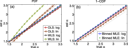
Figure 1: Estimates of $\alpha$ from linearly (lin) and logarithmically (log) binned data using maximum likelihood and both ordinary least-squares (OLS) and weighted least-squares (WLS) linear regression methods, using either (a) the p.d.f. or (b) the complementary c.d.f. We omit error bars when they are smaller than the symbol size. In all cases, the MLE is most accurate, sometimes dramatically so.

Regression can be made to produce accurate estimates, using nonstandard techniques. Aban and Meerschaert (2004) show that their robust least-squares estimator has lesser variance than the $qq$-estimator of Kratz and Resnick (1996) or, equivalently, the exponential tail estimator of Schultze and Steinebach (1996). Surprisingly enough, their estimator equals the Hill estimator [Hill (1975)] which is equivalent to our binned MLE. The computational complexity of this robust least-squares linear regression approach is therefore the same as that of our binned MLE.

3.3 Estimating the lower bound on power-law behavior

For most empirical quantities, the power law holds only above some value, in the upper tail, while the body follows some other distribution. Our goal is not to model the entire distribution, which may have very complicated structure. Instead, we aim for the simpler task of identifying some value $b_{\min}$ above which the power-law behavior holds, estimate the scaling parameter $\alpha$ from those data, and discard the nonpower-law data below it.

The method of choosing $b_{\min}$ has a strong impact on both our estimate for $\alpha$ and the results of our subsequent tests. Choosing $b_{\min}$ too low may bias $\hat{\alpha}$ by including nonpower-law data in the fit, while choosing too high throws away legitimate data and increases our statistical uncertainty. From a practical perspective, we should prefer to be slightly conservative, throwing away some good data if it means avoiding bias. Unfortunately, maximum likelihood fails for estimating the lower bound because $b_{\min}$ truncates the sample and the maximum likelihood choice is always $b_{\min}=b_{k}$, that is, the last bin. Some nonlikelihood-based method must be used. The common approach of choosing $b_{\min}$ by visual inspection on a log–log plot of the empirical data is obviously subjective, and thus should also be avoided.

The approach advocated in Clauset, Shalizi and Newman (2009), originally proposed in Clauset, Young and Gleditsch (2007), is a distance-based method [Reiss and Thomas (2007)] that chooses $x_{\min}$ by minimizing the distributional distance between the fitted model and the empirical data above that choice. This approach has been shown to perform well on both synthetic and real-world data. Other principled approaches exist [Breiman, Stone and Kooperberg (1990), Danielsson et al. (2001), Dekkers and de Haan (1993), Drees and Kaufmann (1998), Handcock and Jones (2004)], although none is universally accepted.

Our recipe for choosing $b_{\min}$ is as follows: [1.]

For each possible $b_{\min}\in(b_{1},b_{2},b_{3},\ldots,b_{k-1})$, estimate $\hat{\alpha}$ using the methods described in Section 3.2 for the counts $h_{\min}$ and higher. (For technical reasons, we require the fit to span at least two bins.)

Compute the Kolmogorov–Smirnov (KS) goodness-of-fit statistic between the fitted c.d.f. and the empirical distribution.

Choose as $\hat{b}_{\min}$ the bin boundary with the smallest KS statistic. The KS statistic is defined in the usual way [Press et al. (1992)]. Let $P(b|\hat{\alpha},b_{\min})$ be the c.d.f. for the binned power law, with parameter $\hat{\alpha}$ and current choice $b_{\min}$, and let $S(b)$ be the cumulative binned empirical distribution for counts in bins $b_{\min}$ and higher. We choose $\hat{b}_{\min}$ as the value that minimizes

$$D=\max_{b\geq b_{\min}}\bigl{|}S(b)-P(b|\alpha,b_{\min})\bigr{|}.$$ (10)

Thus, when $b_{\min}$ is too low, reaching into the nonpower-law portion of the empirical data, the KS distance will be high because the power-law model is a poor fit to those data; similarly, when $b_{\min}$ is too high, the sample size is small and the KS distance will also be high. Both effects are small when $b_{\min}$ coincides with the beginning of the power-law behavior.

To illustrate the accuracy of this method, we compare its performance with the one proposed by Reiss and Thomas (2007). Their methodology (the RT method) selects the bin boundary with index $\min\in\{1,2,3,\ldots,k-1\}$ that minimizes

(12)

(13)

where $(\hat{\alpha}_{\min},\ldots,\hat{\alpha}_{k})$ are the slope estimates calculated by considering data above bin boundaries $(b_{\min},\ldots,b_{k})$, respectively.

The idea behind this approach is to minimize the asymptotic mean squared error in $\hat{\alpha}$ using a finite sample. The choice that yields this minimum is the optimal sample fraction, which is the fraction of observations after $b_{\min}$, and $\beta$ is a smoothing parameter that can be used to improve the choice of $b_{\min}$ for small and medium sized samples.

3.4 Performance of lower bound estimator

We evaluate the accuracy of these two methods using synthetic data drawn from a composite distribution that follows a power law above some choice of $b_{\min}$ but some other distribution below it. We then apply both linear and logarithmic binning schemes, for a variety of choices of the true $b_{\min}$. The form of our test density is

$$p(x)=\cases{Ce^{-{\alpha}(x/b_{\min}-1)},&\quad$b_{1}\leq x<b_{\min},$\vspace*{2pt}\cr C{(x/b_{\min})}^{-\alpha},&\quad$\mbox{otherwise},$}$$ (14)

which has a continuous slope at $b_{\min}$ and thus departs slowly from the power-law form below this point. This provides a difficult task for the estimation procedure.

In our numerical experiments, we fix the sample size at $N=10\mbox{,}000$ and use a linear scheme, $b_{i}=1+50(i-1)$ (constant width of 50), and a logarithmic one, $b_{i}=2^{(i-1)}$ (powers of 2). For our first experiment, we hold the scaling parameter fixed at $\alpha=3$ and characterize each method’s ability to recover the true threshold $b_{\min}$, which we vary across the values of $B$. In a second experiment, we fix $b_{\min}$ at the tenth bin boundary and characterize the impact of misestimating $b_{\min}$ on the estimated scaling parameter, and so vary $\alpha$ over the interval $[1.5,3.5]$.

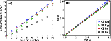
Figure 2: Estimated $b_{\min}$ using the KS-minimization method and the Reiss–Thomas or RT method; (a) the true bin number versus estimated bin number and (b) true $\alpha$ versus $\hat{\alpha}$ for true bin number $10$. In both figures, we show results for logarithmic (log) and linear (lin) binning schemes with $y=x$ (dashed line) shown for reference.

Figure 2(a) shows the results for estimating the threshold, which is reliably identified in the logarithmic binning scheme but slightly underestimated for the KS method and moderately underestimated for the RT method with the linear scheme. However, Figure 2(b) shows that for both methods and binning schemes, if we treat $b_{\min}$ as a nuisance parameter, the scaling parameter itself is accurately estimated.

The slight deviations from the $y=x$ line in both figures highlight some of the pitfalls of working with binned data and power-law distributions. First, in estimating $b_{\min}$ [Figure 2(a)], the linear binning scheme yields a slight but consistent underestimate, thereby including some nonpower-law data in the estimation, while the logarithmic scheme shows no such bias. This arises from the differences in linear versus logarithmic binning. Because logarithmic bins span increasingly large intervals, the distribution’s curvature around $b_{\min}$ is accentuated, presenting a more obvious target for the algorithm, while a linear scheme spreads this curvature across several bins. For both algorithms the choice of $\hat{b}_{\min}$ is slightly below $b_{\min}$, however, this does not induce a substantial bias in $\alpha$, which remains close to the true value [Figure 2(b)].

Second, when the true value is $\alpha\gtrsim 3$, we see a slight underestimation of $\alpha$ for the RT-method caused by the slight underestimate of $b_{\min}$ with this method. However, the RT-method can be shown to work in the limit of large sample size, as this underestimation reduces with a higher $N$. The slight overestimate of $\alpha$ for the KS-method under a logarithmic scheme is caused by a special kind of small sample bias. This bias appears either when the number of observations or the number of bins in the tail region is small.

To illustrate this “few bins” bias, even when sample size is large, we conduct a third experiment: using the same powers-of-two binning scheme, we now fix $b_{\min}=2^{9}$ and $\alpha=3.5$, while varying the sample size $N$. As $N$ increases, a larger number of bins above $b_{\min}$ will be populated, and we measure the accuracy of $\hat{\alpha}$ as this number increases. Figure 3 shows that the bias in $\hat{\alpha}$ decreases with sample size, as we expect, but with a second-order variation that decreases as the average number of bins in the tail region increases. The implication is that researchers must be cognizant of both small sample issues and having too few bins in the scaling region.

Last, obtaining uncertainty in our estimates (${\hat{b}}_{\min}$, $\hat{\alpha}$) can be done using a nonparametric bootstrap method [Efron and Tibshirani (1993)]. Given empirical data with $N$ observations that are binned using a binning scheme $B$, we generate $m$ synthetic data sets in the following way: [1.]

For each data set, we draw $N$ samples $\{x_{1},\ldots,x_{N}\}$ such that the probability of some sample $x_{j}$ being drawn from the $i$th bin is simply the cell probability $h_{i}/N$, where $h_{i}$ is the number of observations in the $i$th bin.

We then bin the samples $\{x_{1},\ldots,x_{N}\}$ using the same binning style $B$. Using these $m$ data sets, we report the standard deviation from $m$ estimates of the model parameters calculated using the methods described above.

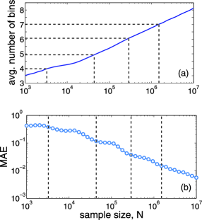
Figure 3: The “few bins” bias; for fixed $\alpha=3.5$, $b_{\min}=2^{9}$ and $c=2$ logarithmic binning scheme, the (a) average number of bins above $b_{\min}$ and (b) mean absolute error, as a function of sample size $N$, illustrating a second-order bias that decreases as the average number of bins in the fitted region increases.

3.5 Slowly varying functions

A function $L(x)$ is said to be slowly varying if

$$\lim_{x\to\infty}\frac{L(cx)}{L(x)}=1$$ (15)

for some constant $c>0$. From the perspective of extreme value theory, we can use this notion to describe a probability density $p(x)$ that asymptotically follows the power law as

$$p(x)\propto L(x)x^{-\alpha}.$$ (16)

The difficulty of using this model when analyzing empirical data is the difficulty of choosing the value of $x$ above which the $x^{-\alpha}$ term starts dominating the above equation, that is, to estimate $x_{\min}$ (or $b_{\min}$ for binned data). A common approach is to visually inspect the plot of the estimate $\hat{\alpha}$ as a function of $b_{\min}$ (called a Hill plot) and identify the point ${\hat{b}}_{\min}$ beyond which $\hat{\alpha}$ appears stable. However, other approaches such as those of Kratz and Resnick (1996) (using a $qq$-plot) and Stoev, Michailidis and Taqqu (2011) (using block-maxima of the data) often yield better results.

The KS method described above can accurately estimate $\hat{b}_{\min}$ when the true $b_{\min}$ lies in the range of the empirical data. Thus, we risk rejecting a true power-law hypothesis, when the empirical distribution follows the power law only for higher $x$ values not seen in the sample or, in other words, when the $L(x)$ term dominates the $x^{-\alpha}$ term for the entire range of the sample. The general solution is to model the structure of $L(x)$ correctly. This is highly nontrivial, as $L(x)$ can have many parametric forms and thus testing for $L(x)$ is difficult. The advantage of our method is that we do not model $L(x)$, as we simply ignore the data below $b_{\min}$. This makes our method inherently conservative, in that we may fail to find a power law in the upper tail because $L(x)$ creates systematic deviations in the observed range.

Note that, in practice, quantities that follow the power law only asymptotically may not appear to follow the power law for a measurable sample of those quantities. Thus, an empirical sample would only be modeled by some $L(x)$ and would not imply the interesting underlying mechanisms that the power laws imply. Thus, if we care only about empirical power-law distributions that can actually be measured, the methods we describe are a reasonable approach.

4 Testing the power-law hypothesis

The methods of Section 3 allow us to accurately fit a power-law tail model to binned empirical data. These methods, however, provide no warning if the fitted model is a poor fit to the data, that is, when the power-law model is not a plausible generating distribution for the observed bin counts. Because a wide variety of heavy-tailed distributions, such as the log-normal and the stretched exponential (also called the Weibull), among others, can produce samples that resemble power-law distributions [see Figure 4(a)], this is a critical question to answer.

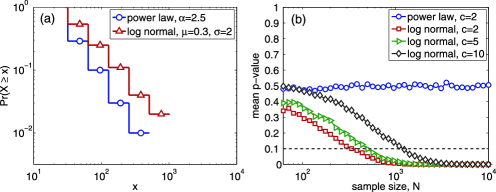
Figure 4: (a) Logarithmic histograms for two $N=100$ samples from a power law and a log-normal distribution. Both exhibit a linear pattern on log–log axes, despite only one being a power law. (b) Mean $p$ for the power-law hypothesis, as a function of sample size $N$; dashed line gives the threshold for rejecting the power law. For power-law data, $p$ is typically high, while for the nonpower-law data, $p$ is a decreasing function of sample size. Notably, the binning scheme’s coarseness determines the sample size required to correctly reject the power-law model.

Toward this end, we adapt the goodness-of-fit test of Clauset, Shalizi and Newman (2009) to the context of binned data. Demonstrating that the power-law model is plausible, however, does not determine whether it is more plausible than alternatives. To answer this question, we adapt the likelihood ratio test of Clauset, Shalizi and Newman (2009) to binned data in Section 5. For both, we additionally explore the impact of information loss from binning on the statistical power of these tests.

4.1 Goodness-of-fit test

Given the observed bin counts and a hypothesized power-law distribution from which the counts were drawn, we would like to know whether the power law is plausible, given the counts.

A goodness-of-fit test provides a quantitative answer to this question in the form of a $p$-value, which in turn represents the likelihood that the hypothesized model would generate data with a more extreme deviation from the hypothesis than the empirical data. If $p$ is large (close to 1), the difference between the data and model may be attributed to statistical fluctuations; if it is small (close to 0), the model is rejected as an implausible generating process for the data. From a theoretical point of view, failing to reject is sufficient license to proceed, provisionally, with considering mechanistic models that assume or generate a power law for the quantity of interest.

The first step of our approach is to fit the power-law model to the bin counts, using methods described in Section 3 to choose $\hat{\alpha}$ and $\hat{b}_{\min}$. Given this hypothesized model $M$, the remaining steps are as follows; in each case, we always use the fixed binning scheme $B$ given to us with the empirical data: [1.]

Compute the distance $D^{*}$ between the estimated model $M$ and the empirical bin counts $H$, using the KS goodness-of-fit statistic, equation (10).

Using a semi-parametric bootstrap, generate a synthetic data set with $N$ values that follows a binned power-law distribution with parameter $\hat{\alpha}$ at and above $\hat{b}_{\min}$, but follows the empirical distribution below $\hat{b}_{\min}$. Call these synthetic bin counts $H^{\prime}$.

Fit the power-law model to $H^{\prime}$, yielding a new model $M^{\prime}$ with parameters $\hat{b}^{\prime}_{\min}$ and $\alpha^{\prime}$.

Compute the distance $D$ between $M^{\prime}$ and $H^{\prime}$.

Repeat steps 2–4 many times, and report $p=\Pr(D\geq D^{*})$, the fraction of these distances that are at least as large at $D^{*}$. To generate synthetic binned data, the semi-parametric bootstrap in step 2 is as follows. Recall that $n$ counts the number of observations from the data $H$ that fall in the power-law region. With probability $n/N$, generate a nonbinned power-law random deviate [Clauset, Shalizi and Newman (2009)] from $M$ and increment the corresponding bin count in the synthetic data set; otherwise, with probability $1-n/N$, increment the count of a bin $i$ below $\hat{b}_{\min}$ chosen with probability proportional to its empirical count $h_{i}$. Repeating this process $N$ times, we generate a complete synthetic data set with the desired properties.

The use of the KS statistic as a goodness-of-fit measure is nontraditional since it gets underestimated for binned data [Noether (1963)]. However, estimating the distribution of distances in step 4 via Monte Carlo allows us to correctly construct the hypothesis test and choose the critical value. [As an example, see Table 2 of Goldstein, Morris and Yen (2004).] This is necessary to produce an unbiased estimate of $p$ because our original model parameters $M$ are estimated from the empirical data. The semi-parametric bootstrap ensures that the subsequent values $D$ are estimated in precisely the same way—by estimating both $b_{\min}$ and $\alpha$ from the synthetic data—that we estimated $D^{*}$ from $H$. Failure to estimate $\hat{b}^{\prime}_{\min}$ from $H^{\prime}$, using $\hat{b}_{\min}$ from $H$ instead, yields a biased and thus unreliable $p$-value.

How many such synthetic data sets should we generate? The answer given by Clauset, Shalizi and Newman (2009) also holds in the case of binned data. We should generate at least $\frac{1}{4}\varepsilon^{-2}$ synthetic data sets to achieve an accuracy of knowing $p$ to within $\varepsilon$ of the true value. For example, if we wish to know $p$ to within $\varepsilon=0.01$, we should generate about 2500 synthetic data sets.

Given an estimate of $p$, we must decide if it is small enough to reject the power-law hypothesis. We recommend the relatively conservative choice of ruling out the power law if $p<0.1$. By not using smaller rejection thresholds, we avoid letting through some quantities that in fact have only a small chance of actually following a power law.

Note that a large value of $p$ does not imply the correctness of the power law for the data. A large $p$ can arise for at least two reasons. First, there may be alternative distributions that fit the data as well or better than the power law, and other tests are necessary to make this determination (which we cover in Section 5). Second, for small values of $n$, or for a small number of bins above $b_{\min}$, the empirical distribution may closely follow a power-law shape, yielding a large $p$, even if the underlying distribution is not a power law. This happens not because the goodness-of-fit test is deficient, but simply because it is genuinely hard to rule out the power law if we have very little data. For this reason, a large $p$ should be interpreted cautiously either if $n$ or the number of bins in the fitted region is small.

Finally, we do not recommend the use of the well-known $\chi^{2}$ statistic for analyzing heavy-tailed distributions, since it requires the expected cell frequencies to be above a certain threshold [Tate and Hye (1973)] and has less statistical power compared to the KS statistic [Horn (1977)].

4.2 Performance of the goodness-of-fit test

To demonstrate the effectiveness of our goodness-of-fit test for binned data, we drew various-sized synthetic data from two distributions: a power law with $\alpha=2.5$ and a log-normal distribution with $\mu=0.3$ and $\sigma=2.0$, both with $b_{\min}=16$. Using these methods, one can compare against any other alternative distribution. However, the choice of log-normal provides a strong test because for a wide range of sample sizes it produces bin counts that are reasonably power-law-like when plotted on log–log axes [Figure 4(a)].

Figure 4(b) shows the average $p$-value, as a function of sample size $N$, for the power-law hypothesis when data are drawn from these distributions. When we fit the correct model to the data, the resulting $p$-value is uniformly distributed, and the mean $p$-value is $0.5$, as expected. When applied to log-normal data, however, the $p$-value remains above our threshold for rejection only for small samples ($N\lesssim 300$), and we correctly reject the power law for larger samples. We note, however, that the sample size at which the $p$-value leads to a correct rejection of the power law depends on the binning scheme, requiring a larger sample size when the binning scheme is more coarse (larger $c$).

5 Alternative distributions

The methods described in Section 4 provide a way to test whether our binned data plausibly follow a power law. However, many distributions, not all of them heavy tailed, can produce data that appear to follow a power law when binned. A large $p$-value for the power-law model provides no information about whether some other distribution might be an equally plausible or even a better explanation. Demonstrating that such alternatives are worse models of the data strengthens the statistical argument in favor of the power law.

There are several principled approaches to comparing the power-law model to alternatives, for example, cross-validation [Stone (1974)], minimum description length [Grünwald (2007)] or Bayesian techniques [Kass and Raftery (1994)]. Following Clauset, Shalizi and Newman (2009), we construct a likelihood ratio test proposed by Vuong (1989) (LRT) for binned data. This approach has several attractive features, including the ability to fail to distinguish between the power law and an alternative, for example, due to small sample sizes. Information loss from binning reduces the statistical power of the LRT and, thus, its results for binned data should be interpreted cautiously. Further, although there are generally an unlimited number of alternative models, only a few are commonly proposed alternatives or correspond to common theoretical mechanisms. We focus our efforts on these, although in specific applications, a researcher must use their expert judgement as to what constitutes a reasonable alternative.

In what follows, we will consider four alternative distributions, the exponential, the log-normal and the stretched exponential (Weibull) distribution, plus a power-law distribution with exponential cutoff. Table 1 gives the mathematical forms of these models. In application to binned data, a piecewise integration over bins, like equation (2), was carried out and parameters were estimated by numerically maximizing the log-likelihood function.

Table 1: Definitions of alternative distributions for our likelihood ratio tests. For each, we give the basic functional form $f(x)$ and the appropriate normalization constant $C$ such that $\int_{x_{\min}}^{\infty}Cf(x)\,\mathrm{d}x=1$ for the continuous case

	Density $\bolds{p(x)=Cf(x)}$
Name	$\bolds{f(x)}$	$\bolds{C}$
Power law with cutoff	$x^{-\alpha}\mathrm{e}^{-\lambda x}$	${\lambda^{1-\alpha}\over\Gamma(1-\alpha,\lambda x_{\min})}$
Exponential	$\mathrm{e}^{-\lambda x}$	$\lambda\mathrm{e}^{\lambda x_{\min}}$
Stretched exponential	$x^{\beta-1}\mathrm{e}^{-\lambda x^{\beta}}$	$\beta\lambda\mathrm{e}^{\lambda x_{\min}^{\beta}}$
Log-normal	${1\over x}\exp[-{(\ln x-\mu)^{2}\over 2\sigma^{2}}]$	$\sqrt{{2\over\pi\sigma^{2}}}[\mathop{\operatorname{erfc}}({\ln x_{\mathrm{min}}-\mu\over\sqrt{2}\sigma})]^{-1}$

5.1 Direct comparison of models

Given a pair of parametric models $A$ and $B$ for which we may compute the likelihood of our binned data, the model with the larger likelihood is a better fit. The logarithm of the ratio of the two likelihoods $\mathcal{R}$ provides a natural test statistic for making this decision: it is positive or negative depending on which distribution is better, and it is indistinguishable from zero in the event of a tie.

Because our empirical data are subject to statistical fluctuations, the sign of $\mathcal{R}$ also fluctuates. Thus, its direction should not be trusted unless we may determine that its value is probably not close to $\mathcal{R}=0$. That is, in order to make a firm choice between distributions, we require a log-likelihood ratio that is sufficiently positive or negative that it could not plausibly be the result of a chance fluctuation from zero.

The log-likelihood ratio is defined as

$${\mathcal{R}}=\ln\biggl{(}\frac{{\mathcal{L}_{A}}(H|{\hat{\theta}}_{A})}{{\mathcal{L}_{B}}(H|{\hat{\theta}}_{B})}\biggr{)},$$ (24)

where by convention $\mathcal{L}_{A}$ is the likelihood of the model under the power-law hypothesis, fitted using the methods in Section 3, and $\mathcal{L}_{B}$ is the likelihood under the alternative distribution, again fitted by maximum likelihood. To guarantee the comparability of the models, we further require that they be fitted to the same bin counts, that is, to those at or above $\hat{b}_{\min}$ chosen by the power-law model.

Given $\mathcal{R}$, we use the method proposed by Vuong [Vuong (1989)] to determine if the observed sign of $\mathcal{R}$ is statistically significant. This yields a $p$-value: if $p$ is small (say, $p<0.1$), then the observed sign is not likely due to chance fluctuations around zero; if $p$ is large, then the sign is not reliable and the test fails to favor one model over the other. Technical details of the likelihood ratio test are given in the supplementary material [Virkar and Clauset (2014)] (Section 2). Results from Clauset, Shalizi and Newman (2009) show that this hypothesis test substantially increases the reliability of the likelihood ratio test, yielding accurate answers for much smaller data sets than if the sign is interpreted without regard to its statistical significance.

Before evaluating the performance of the LRT on binned data, we make a few cautionary remarks about nested models. When one model is strictly a subset of the other, as in the case of a power law and a power law with exponential cutoff, even if the smaller model is the true model, the larger model will always yield at least as large a likelihood. In this case, we must slightly modify the hypothesis test for the sign of $\mathcal{R}$ and use a little more caution in interpreting the results; see supplementary material [Virkar and Clauset (2014)] (Section 2).

5.2 Performance of the likelihood ratio test

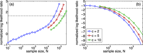
Figure 5: Behavior of normalized log-likelihood ratio $n^{-1/2}\mathcal{R}/\sigma$, for synthetic data sets drawn from (a) power-law and (b) log-normal distributions. Both were then binned using a logarithmic binning scheme, with bin boundaries in powers of $c=\{2,5,10\}$. Dashed line indicates the threshold at which the sign of $n^{-1/2}\mathcal{R}/\sigma$ becomes trustworthy.

We demonstrate the performance of the likelihood ratio test for binned data by pitting the power-law hypothesis against the log-normal hypothesis. For a log-normal distribution, increasing the $\sigma$ parameter results in a power-law-like region for a large range. Thus, in general, rejecting a log-normal hypothesis in favor of a power-law hypothesis using any model comparison test is a difficult task, made all the more difficult when the data are binned (see Section 6). We also note that since a power law implies different generative mechanisms as opposed to a log normal [Mitzenmacher (2004)], favoring one hypothesis over the other has important scientific implications for understanding what processes generated the data.

To illustrate these points, we conduct two experiments: one in which we draw a sample from a power-law distribution, with $\alpha=2.5$ and $x_{\min}=1$, and a second in which we draw a sample from a log-normal distribution, with $\mu=0.3$ and $\sigma=2$. We then bin these samples logarithmically, with $c=\{2,5,10\}$, and fit and compare the power-law and log-normal models. The normalized log-likelihood ratio $n^{-1/2}\mathcal{R}/\sigma$ (see Section 2 of the supplementary material [Virkar and Clauset (2014)]) provides a concrete measure by which to compare outcomes at different sample sizes. If the test performs well, in the first case, $\mathcal{R}$ will tend to be positive, correctly favoring the power law as the better model, while in the second, the ratio will tend to be negative, correctly rejecting the power law.

Figure 5 shows the results. When the power-law hypothesis is correct [Figure 5(a)], the sign of $\mathcal{R}$ allows us to correctly rule in favor of the power law when the sample size is sufficiently large. However, the size required for an unambiguously correct decision grows with the coarseness of the binning scheme (larger $c$). Interestingly, a reliably correct decision in favor of the power law [Figure 5(a)] requires a much larger sample size ($n\approx 20\mbox{,}000$ here) than a decision against it [Figure 5(b)] ($n\lesssim 200$). This illustrates the difficulty of rejecting alternative distributions like the log-normal, which can imitate a power law over a wide range of sample sizes.

6 Information loss due to binning

The above results already demonstrate that binned data can make accurately fitting and testing the power-law hypothesis more difficult. Figure 1 of the supplementary material [Virkar and Clauset (2014)] and Figures 4 and 5 show that all the three steps of our framework have reduced statistical power if we use coarser binning schemes. In this section we quantify the impact of different binning schemes on both the statistical and model uncertainty for the power-law hypothesis.

To illustrate this loss of information, we pose the following question: Suppose we have a sample $n_{1}\to\infty$ and a binning scheme $c_{1}$ (logarithmic in powers of $c_{1}$). Given a choice of $\alpha$, how much larger a sample do we need in order to achieve the same statistical accuracy in $\hat{\alpha}$ using a coarser scheme $c_{2}>c_{1}$?

In the limit of large sample size, the asymptotic variance is equal to the inverse of Fisher information [see Cramér (1946), Rao (1947)]. For the two different binning schemes ($c_{1}$, $c_{2}$) and the corresponding sample sizes ($n_{1},n_{2}$), the following approximate equality holds (see Section 1.2 of the supplementary material [Virkar and Clauset (2014)]) for the sample size in question, that is, $n_{2}$:

$$n_{2}=\biggl{(}\biggl{(}\frac{c_{1}}{c_{2}}\biggr{)}^{1+\alpha}{\biggl{(}\frac{\ln c_{1}}{\ln c_{2}}\biggr{)}}^{2}{\biggl{(}\frac{c_{2}-{c_{2}}^{\alpha}}{c_{1}-{c_{1}}^{\alpha}}\biggr{)}}^{2}\biggr{)}n_{1}.$$ (25)

Figure 6 illustrates how $n_{2}$ varies with the coarseness of the second binning scheme $c_{2}$. For concreteness, we fix $c_{1}=2$ and show the constant’s behavior for several choices of $\alpha$ and for schemes $c_{2}\geq 2$. As expected, increasing the coarseness of the binning scheme decreases the information available for estimation, and the required sample size increases. Information loss also arises from variation in $\alpha$. As $\alpha$ increases, the variance of the generating distribution decreases, and a given sample size will span fewer bins. The fundamental source of information loss for estimation is the loss of bins, that is, the commingling of observations that are distinct, which may arise either from coarsening the binning scheme or from decreasing the variance of the generating distribution.

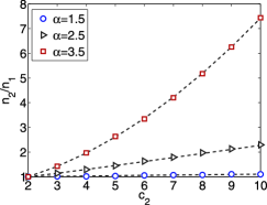
Figure 6: The size of a data set required to achieve the same statistical certainty in $\alpha$ (constant MSE) when using a coarser binning scheme $c_{2}$, for several choices of $\alpha$. Since our claim here is asymptotic, fixing a large value for $n_{1}$ (e.g., $10^{4}$) results in a good agreement between the data points that come from a simulation study and the dashed lines obtained analytically from equation (25)

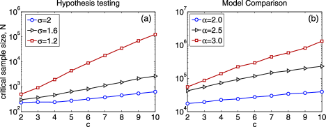
Figure 7: Impact of information loss on: (a) mean $p$-value using synthetic log-normal data and (b) normalized log-likelihood ratio $n^{-1/2}\mathcal{R}/\sigma$ using synthetic power-law data. All data sets are logarithmically binned in powers of $c$ shown on the $x$-axis. We show the critical value of the sample size, $N$, required to make the correct decision for both these steps of our framework on the $y$-axis.

The information-loss effect is sufficiently strong that a powers-of-10 binning scheme can require nearly eight times as large a sample to obtain the same statistical accuracy in $\alpha$, when $\alpha>3$. Thus, if the option is available during the experimental design phase of a study, as fine a grained binning scheme as is possible should be used in collecting the data in order to maximize subsequent statistical accuracy.

We now illustrate the impact of loss of bins on the hypothesis testing and the model comparison steps of our framework, respectively, using two experiments: one in which we draw a sample from a log-normal distribution with $\mu=0.3$ and $\sigma=\{1.2,1.6,2\}$ and second in which we draw a sample from the power-law distribution with $\alpha=\{2,2.5,3\}$. We keep $b_{\min}$ fixed for both the experiments. In the first experiment, we test the plausibility of the power-law hypothesis by computing the mean $p$-value and in the second experiment, we compare the power-law and the log-normal hypotheses by computing the normalized log-likelihood ratio.

We show the critical sample size, $N$, required to reject the power-law hypothesis in the first experiment [Figure 7(a)] and to favor the power-law hypothesis in the second experiment [Figure 7(b)] as a function of the binning scheme $c$. We also study the effect of variance of the underlying distribution by showing the trend lines for $\sigma$ and $\alpha$, respectively, for the two figures. Here again we observe that decreasing the variance (i.e., decreasing $\sigma$ for the log normal or increasing $\alpha$ for the power law) results in loss of bins and, hence, larger $N$ is required to reliably make the correct decision. Increasing $c$ has a similar effect. Note that decreasing variance corresponds to the rate at which $N$ has to be increased for making correct decisions.

7 Applications to real-world data

Having described statistically principled methods for working with power-law distributions and binned empirical data, we now apply them to analyze several real-world binned data sets to determine which of them do and do not follow power-law distributions. As we will see, the results indicate that some of these quantities are indeed consistent with the power-law hypothesis, while others are not.

The 12 data sets we study are drawn from a broad variety of scientific domains, including medicine, genetics, geology, ecology, meteorology, earth sciences, demographics and the social sciences. They are as follows: [10.]

Estimated number of personnel in a terrorist organization [Asal and Rethemeyer (2008)], binned by powers of ten, expect that the first two bins are merged.

Diameter of branches in the plant species Cryptomeria [Shinokazi et al. (1964)], binned in 30 mm intervals.

Volume of ice in an iceberg calving event [Chapuis and Tetzlaff (2012)], binned by powers of ten.

Length of a patient’s hospital stay within a year [Heritage Provider Network (2012)], arbitrarily binned as natural numbers from 1 to 15, plus one bin spanning 16–365 days. (Stays of length 0 are omitted.)

Wind speed (mph) of a tornado in the United States from 2007 to 2011 [Storm Prediction Center (2011)], binned into categories according to the Enhanced Fujita (EF) scale, a roughly logarithmic binning scheme.

Maximum wind speed (knots) of tropical storms and hurricanes in the United States between 1949 and 2010 [Jarvinen, Neumann and Davis (2012)], binned in 5-knot intervals.

The human population of U.S. cities in the 2000 U.S. Census.

Size (acres) of wildfires occurring on U.S. federal land from 1986–1996 [Newman (2005)].

Intensity of earthquakes occurring in California from 1910–1992, measured as the maximum amplitude of motion during the quake [Newman (2005)].

Area (sq. km) of glaciers in Scandinavia [World Glacier Monitoring Service and National Snow and Ice Data Center (2012)].

Number of cases per 100,000 of various rare diseases [Orphanet Report Series, Rare Diseases collection (2011)].

Number of genes associated with a disease [Goh et al. (2007)].

= Quantity $\bolds{N}$ Binning scheme $\bolds{B}$ $\bolds{\hat{\alpha}}$ Std. err. $\bolds{\hat{b}_{\min}}$ $\bolds{n}$, tail $\bolds{p(\pm 0.03)}$ Personnel in a terrorist group 393 logarithmic, $c=10$ $1.75$ (0.11)0 1000 56 0.13 — $1.29$ (0.01)0 $\circ$ 1 393 0.00 Plant branch diameter (mm) 3897 linear, 30 mm $2.34$ (0.02)0 0.3 3897 0.00 Volume in iceberg calving ($\times 10^{3}$ m³) 5837 arbitrary $1.29$ (0.02)0 $1.26\times 10^{12}$ 143 0.49 — $1.155$ (0.002) $\circ$ $10.97$ 5837 0.00 Length of hospital stay 11,769 arbitrarytt21 $3.24$ (0.27)0 14 303 0.40 — $2.020$ (0.007) $\circ$ 1 11,769 0.00 Wind speed, tornado (mph) 7231 EF-scalett22 $7.10$ (0.20)0 111 980 0.03 — $4.58$ (0.03)0 $\circ$ 65 7231 0.00 Max. wind speed, hurricane (knots) 879 linear, 5 knots $14.20$ (1.69)0 122.5 56 0.36 — $2.44$ (0.03)0 $\circ$ 32.5 879 0.00 Population of city 19,447 logarithmic, $c=2$ $2.38$ (0.07)0 65,536 426 0.72 Size of wildfire (acres) 203,785 logarithmic, $c=2$ $1.482$ (0.002) 2 52,004 0.00 Intensity of earthquake 19,302 logarithmic, $c=10$ $1.82$ (0.02)0 10,000 2659 0.18 Size of glacier (km²) 2428 logarithmic, $c=2$ $1.95$ (0.04)0 1 635 0.04 Rare disease prevalence 675 logarithmic, $c=2$ $2.88$ (0.14)0 16 99 0.00 Genes associated with disease 1284 logarithmic, $c=2$ $2.72$ (0.12)0 8 217 0.87 — $1.75$ (0.01)0 $\circ$ 1 1284 0.00 [a]tt21[Heritage Provider Network (2012)]. [b]tt22[Storm Prediction Center (2011)].

Table 2: Details of the data sets described in Section 7, along with their power-law fits and the corresponding $p$-values (bold values indicate statistically plausible fits). $N$ denotes the full sample size, while $n$ is the size of the fitted power-law region. Cases where we additionally considered a restricted power-law fit (see text), with fixed $b_{\min}=b_{1}$, are denoted by $\circ$ next to the $\hat{b}_{\min}$ value. Standard error (std. err.) estimates were derived from a bootstrap using 1000 replications

Data sets 1–6 are naturally binned, that is, bins are fixed as given and either the raw observations are unavailable or analyses of such data typically focus on binned observations. Raw values for data sets 7–12 are available, and these quantities are included for other reasons. Data sets 7–9 were also analyzed in Clauset, Shalizi and Newman (2009), and we reanalyze them in order to illustrate that similar conclusions may be extracted despite binning or to highlight differences induced by binning. Data sets 10–12 were analyzed as binned data by their primary sources, and we do the same to ensure comparability of our results.

Table 2 summarizes each data set and gives the parameters of the best fitting power law. Figures 8 and 9 plot the empirical bin counts and the fitted power-law models. In several cases, we also include fits where we have fixed $b_{\min}=b_{1}$, the smallest bin boundary in order to test the power-law model on the entire data set. This supplementary test was conducted when either a previous claim had been made regarding the entire distribution’s shape or when visual inspection suggested that such a claim might be reasonable. Finally, Table 3 summarizes the results of the likelihood ratio tests and includes our judgement of the statistical support for the power-law hypothesis with each data set.

For none of the quantities was the power-law hypothesis strongly supported, which requires that the power law was both a good fit to the data and a better fit than the alternatives. This fact reinforces the difficulty of distinguishing genuine power-law behavior from nonpower-law-but-still-heavy-tailed behavior. In most cases, the likelihood ratio test against the exponential distribution confirms the heavy-tailed nature of these quantities, that is, the power law was typically a better fit than the exponential, except for the length of hospital stays, tornado wind speeds and the prevalences of rare diseases.

Two quantities—the number of personnel in a terrorist organization and the number of genes associated with a disease—yielded weak support for the power-law hypothesis, in which the power law was a good fit, but at least one alternative was better. In the case of the gene-disease data, this quantity is better fit by a log-normal distribution, suggesting some kind of multiplicative stochastic process as the underlying mechanism. The terror personnel data is better fit by both the log-normal and the stretched exponential distributions, however, given that so few observations ended up in the tail region, the case for any particular distribution is not strong.

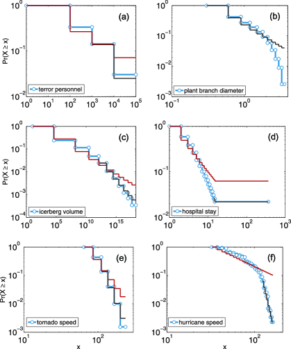
Figure 8: Empirical distributions (as complementary c.d.f.s) $\Pr(X\geq x)$ for data sets 1–6: the (a) number of personnel in a terrorist organization, (b) diameter of branches in plants of the species Cryptomeria, (c) volume of ice in an iceberg calving event, (d) length of a patient’s hospital stay, (e) wind speed of tornados, and (f) maximum wind speed of tropical storms and hurricanes, along with the best fitting power-law distribution with $b_{\min}$ estimated (black) and $b_{\min}$ fixed at the smallest bin boundary (red).

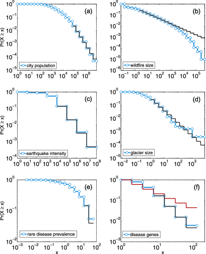
Figure 9: Empirical distributions (as complementary c.d.f.s) $\Pr(X\geq x)$ for data sets 7–12: the (a) human population of U.S. cities, (b) size of wildfires on U.S. federal land, (c) intensity of earthquakes in California, (d) area of glaciers in Scandanavia, (e) prevalence of rare diseases, and (f) number of genes associated with a disease, along with the best fitting power-law distribution with $b_{\min}$ estimated (black) and $b_{\min}$ fixed at the smallest bin boundary (red).

Five quantities produced moderate support for the power law hypothesis, in which the power law was a good fit but alternatives like the log-normal or stretched exponential remain plausible, that is, their likelihood ratio tests were inconclusive. In particular, the volume of icebergs, the length of hospital stays (but see above), the maximum wind speed of a hurricane, the population of a city and the intensity of earthquakes all have moderate support.

Of the six supplemental tests we conducted, in which we fixed $b_{\min}=b_{1}$, only two—the maximum wind speed of hurricanes and the size of wildfires—yielded any support for a power law, and in both cases the power-law distribution with exponential cutoff was better than the pure power law. In the case of hurricanes, a cutoff is scientifically reasonable: windspeed in hurricanes is related to their spatial size, which is ultimately constrained by the size of convection cells in the upper atmosphere, the distribution of the continents and the rate at which energy is transferred from the ocean surface [Persing and Montgomery (2003)]. The presence of such physical constraints implies that any scale invariance present in the underlying generative process must be truncated by the finite size of the Earth itself. Larger planets, like Jupiter and Saturn, may thus exhibit scaling over a larger range of storm intensities, although we know of no systematic data set of extraterrestrial storms.

= Log-normal Exponential Stretched exp. Power law${}\bolds{+}{}$cutoff Quantity Power law $\bolds{p}$ LR $\bolds{p}$ LR $\bolds{p}$ LR $\bolds{p}$ LR $\bolds{p}$ Support for power law Personnel in a terrorist group 0.13 $\mbox{ }-2.01$ 0.04 $3.91$ 0.00 $-1.93$ 0.05 $-2.57$ 0.11 weak — 0.00 $-4.32$ 0.00 $4.59$ 0.00 $-4.47$ 0.00 $-26.26$ 0.00 none Plant branch diameter 0.00 $-9.71$ 0.00 $1.99$ 0.05 $-9.48$ 0.00 $-123.8$ 0.00 none Volume in iceberg calving 0.49 $-1.12$ 0.26 $10.61$ 0.00 $-1.16$ 0.24 $-1.70$ 0.19 moderate — 0.00 $0.85$ 0.40 $43.02$ 0.00 $\mbox{ }2.26$ 0.01 $-13.29$ 0.00 none Length of hospital stay 0.40 $-0.98$ 0.33 $-1.02$ 0.31 $-1.01$ 0.31 $-0.23$ 0.63 moderate — 0.00 $-18.37$ 0.00 $-1.86$ 0.06 $-18.69$ 0.00 $-602.9$ 0.00 none Wind speed, tornado 0.03 $-3.16$ 0.00 $-3.32$ 0.00 $-2.72$ 0.01 $-7.92$ 0.01 none — 0.00 $-17.36$ 0.00 $-19.22$ 0.00 $-13.85$ 0.00 $-214.6$ 0.00 none Max. wind speed, hurricane 0.36 $-0.35$ 0.73 $6.17$ 0.00 $-0.72$ 0.48 $-0.30$ 0.60 moderate — 0.00 $-13.26$ 0.00 $-20.71$ 0.00 $-13.78$ 0.00 $-117.1$ 0.00 with cutoff Population of city 0.72 $-0.07$ 0.95 $16.25$ 0.00 $-0.08$ 0.94 $-0.23$ 0.63 moderate Size of wildfire 0.00 $-16.03$ 0.00 $9.26$ 0.00 $-16.42$ 0.00 $-410$ 0.00 with cutoff Intensity of earthquake 0.18 $1.02$ 0.27 $\mbox{ }21.63$ 0.00 $0.75$ 0.45 $-0.78$ 0.38 moderate Size of glacier 0.04 $-0.56$ 0.58 $1.01$ 0.31 $-0.56$ 0.58 $0.00$ 0.96 none Rare disease prevalence 0.00 $-4.72$ 0.00 $-4.64$ 0.00 $-3.77$ 0.00 $-7.55$ 0.01 none Genes associated with disease 0.87 $-2.52$ 0.01 $2.92$ 0.00 $-0.49$ 0.63 $-0.51$ 0.48 weak — 0.00 $-11.28$ 0.00 $-3.14$ 0.00 $-10.83$ 0.00 $-159.4$ 0.00 none

Table 3: Comparison of the fitted power-law behavior against alternatives. For each data set, we give the power law’s $p$-value from Table 2, the log-likelihood ratios against alternatives, and the $p$-value for the significance of each likelihood ratio test. Statistically significant values are given in bold. Positive log-likelihood ratios indicate that the power law is favored over the alternative. For nonnested alternatives, we report the normalized log-likelihood ratio $n^{-1/2}\mathcal{R}\sigma$; for nested models (the power law with exponential cutoff), we give the actual log-likelihood ratios. The final column lists our judgement of the statistical support for the power-law hypothesis with each data set. “None” indicates data sets that are probably not power-law distributed; “weak” indicates that the power law is a good fit but a nonpower law alternative is better; “moderate” indicates that the power law is a good fit but alternatives remain plausible. No quantity achieved a “good” label, where the power law is a good fit and none of the alternatives is considered plausible. In some cases, we write “with cutoff” to indicate that the power law with exponential cutoff is clearly favored over the pure power law. In each of these cases, however, some of the alternatives are also good fits, such as the log-normal and stretched exponential

For the three data sets also analyzed in Clauset, Shalizi and Newman (2009)—city populations, wildfire sizes and earthquake intensities—we reassuringly come to similar conclusions when analyzing their binned counterparts. The one exception is the intensity of earthquakes, which illustrates the impact of information loss from binning. The first consequence is that our choice $b_{\min}$ is slightly larger than the $x_{\min}$ estimated from the raw data. The slight curvature in this distribution’s tail means this difference raises our scaling parameter estimate to $\hat{\alpha}=1.82\pm 0.02$ compared to $\hat{\alpha}=1.64\pm 0.04$ in Clauset, Shalizi and Newman (2009). Furthermore, Clauset, Shalizi and Newman (2009) found the power law to be a poor fit by itself ($p=0.00\pm 0.03$) and that the power-law with a cutoff was heavily favored. In contrast, we failed to reject the power law ($p=0.18\pm 0.03$) and the comparison to the power law with cutoff was inconclusive. That is, the information lost by binning obscured the more clearcut results obtained on raw data for earthquake intensities.

In some cases, our conclusions have direct implications for theoretical work, shedding immediate light on what type of theoretical explanations should or should not be considered for the corresponding phenomena. An illustrative example is the branch diameter data. Past work on the branching structure of plants [Yamamoto and Kobayashi (1993), Shinokazi et al. (1964), West, Enquist and Brown (2009)] has argued for a fractal model, in which certain conservation laws imply a power-law distribution for branch diameters within a plant. Some theories go further, arguing that a forest is a kind of a “scaled up” plant and that the power-law distribution of branch diameters extends to entire collections of naturally co-occuring plants. Critically, the branch data analyzed here, and its purported power-law shape, have been cited as evidence supporting these claims [West, Enquist and Brown (2009)]. However, our results show that these data provide no statistical support for the power-law hypothesis [we find similar results for the other binned data of Shinokazi et al. (1964), West, Enquist and Brown (2009)]. Our results thus demonstrate that these theories’ predictions do not match the empirical data and alternative explanations should be considered. Indeed, our results suggest that the basic pipe model itself is flawed or incomplete, as we observe too few large-diameter branches and too many small-diameter branches compared to the theory’s prediction.

In other cases, our results suggest specific theoretical processes to be considered. For instance, the full distribution of hospital stays is better fit by all the alternative distributions than by the power law, but the stretched exponential is of particular interest. Survival analysis is often framed in terms of hazard rates, that is, a Poisson process with a nonstationary event probability, and our results suggest that such a model may be worth considering: if the hazard rate for leaving the hospital decreases as the length of the stay increases, a heavy-tailed distribution like the stretched exponential is produced. Additional investigation of the covariates that best predict the trajectory of this hazard rate would provide a test of this hypothesis.

8 Conclusions

The primary goal of this article was to introduce a principled framework for testing the power-law hypothesis with binned empirical data, based on the framework introduced in Clauset, Shalizi and Newman (2009), and to explore the impact of information loss due to binning on the resulting statistical conclusions. Although the information loss can be severe for coarse binning schemes, for example, powers-of-10, sound statistical conclusions can still be made using these methods. These methods should allow practitioners in a wide variety of fields to better distinguish power-law from nonpower-law behavior in empirical data, regardless of whether the data are binned or not.

In applying our methods to a large number of data sets from various fields, we found that the data for many of these quantities are not compatible with the hypothesis that they were drawn from a power-law distribution. In a few cases, the data were found to be compatible, but not fully: in these cases, there was ample evidence that alternative heavy-tailed distributions are an equally good or better explanation.

The study of power laws is an exciting effort that spans many disciplines, and their identification in complex systems is often interpreted as evidence for, or suggestions of, theoretically interesting processes. In this paper, we have argued that the common practice of identifying and quantifying power-law distributions by the approximately straight-line behavior on a binned histogram on a doubly logarithmic plot should not be trusted: such straight-line behavior is a necessary but not sufficient condition for true power-law behavior. Furthermore, binned data present special problems because conventional methods for testing the power-law hypothesis [Clauset, Shalizi and Newman (2009)] could only be applied to continuous or integer-valued observations. By extending these techniques to binned data, we enable researchers to reliably investigate the power-law hypothesis even when the data do not take a convenient form, either because of the way they were collected, because the original values are lost, or for some other reason.

Properly applied, these methods can provide objective evidence for or against the claim that a particular distribution follows a power law. (In principle, our binned methods could be extended to other, nonpower-law distributions, although we do not provide such extensions here.) Such objective evidence provides statistical rigor to the larger goal of identifying and characterizing the underlying processes that generate these observed patterns. That being said, answers to some questions of scientific interest may not depend solely on the distribution following a power law perfectly. Whether or not a quantity not following a power law poses a problem for a researcher depends largely on his or her scientific goals, and in some cases a power law may not be more fundamentally interesting than some other heavy-tailed distribution such as the log-normal or the stretched-exponential.

In closing, we emphasize that the identification of a power law in some data is only part of the challenge we face in explaining their causes and implications in natural and man-made phenomena. We also need methods by which to test the processes proposed to explain the observed power laws and to leverage these interesting patterns for practical purposes. This perspective has a long and ongoing history, reaching at least as far back as Ijiri and Simon (1977), with modern analogs given by Mitzenmacher (2006) and by Stumpf and Porter (2012). We hope the statistical tools presented here aid in these endeavors.

References

- Aban and Meerschaert (2004) {barticle}[mr] \bauthor\bsnmAban, \bfnmInmaculada B.\binitsI. B. and \bauthor\bsnmMeerschaert, \bfnmMark M.\binitsM. M. (\byear2004). \btitleGeneralized least-squares estimators for the thickness of heavy tails. \bjournalJ. Statist. Plann. Inference \bvolume119 \bpages341–352. \biddoi=10.1016/S0378-3758(02)00419-6, issn=0378-3758, mr=2019645 \bptokimsref\endbibitem
- Arnold (1983) {bbook}[mr] \bauthor\bsnmArnold, \bfnmBarry C.\binitsB. C. (\byear1983). \btitlePareto Distributions. \bseriesStatistical Distributions in Scientific Work \bvolume5. \bpublisherInternational Co-operative Publishing House, \blocationBurtonsville, MD. \bidmr=0751409 \bptokimsref\endbibitem
- Asal and Rethemeyer (2008) {barticle}[author] \bauthor\bsnmAsal, \bfnmV.\binitsV. and \bauthor\bsnmRethemeyer, \bfnmR. K.\binitsR. K. (\byear2008). \btitleThe nature of the beast: Organizational structures and the lethality of terrorist attacks. \bjournalThe Journal of Politics \bvolume70 \bpages437–449. \bptokimsref\endbibitem
- Barndorff-Nielsen and Cox (1995) {bbook}[author] \bauthor\bsnmBarndorff-Nielsen, \bfnmO. E.\binitsO. E. and \bauthor\bsnmCox, \bfnmD. R.\binitsD. R. (\byear1995). \btitleInference and Asymptotics. \bpublisherChapman & Hall, \blocationLondon. \bptokimsref\endbibitem
- Beirlant and Teugels (1989) {barticle}[author] \bauthor\bsnmBeirlant, \bfnmJ.\binitsJ. and \bauthor\bsnmTeugels., \bfnmJ. L.\binitsJ. L. (\byear1989). \btitleAsymptotic normality of Hill’s estimator. \bjournalExtreme Value Theory \bvolume51 \bpages148–155. \bptokimsref\endbibitem
- Breiman, Stone and Kooperberg (1990) {barticle}[mr] \bauthor\bsnmBreiman, \bfnmLeo\binitsL., \bauthor\bsnmStone, \bfnmCharles J.\binitsC. J. and \bauthor\bsnmKooperberg, \bfnmCharles\binitsC. (\byear1990). \btitleRobust confidence bounds for extreme upper quantiles. \bjournalJ. Stat. Comput. Simul. \bvolume37 \bpages127–149. \biddoi=10.1080/00949659008811300, issn=0094-9655, mr=1082452 \bptokimsref\endbibitem
- Cadez et al. (2002) {barticle}[author] \bauthor\bsnmCadez, \bfnmI. V.\binitsI. V., \bauthor\bsnmSmyth, \bfnmP.\binitsP., \bauthor\bsnmMcLachlan, \bfnmG. J.\binitsG. J. and \bauthor\bsnmMcLaren, \bfnmC. E.\binitsC. E. (\byear2002). \btitleMaximum likelihood estimation of mixture of densities for binned and truncated multivariate data. \bjournalMachine Learning \bvolume47 \bpages7–34. \bptokimsref\endbibitem
- Chapuis and Tetzlaff (2012) {bmisc}[author] \bauthor\bsnmChapuis, \bfnmA.\binitsA. and \bauthor\bsnmTetzlaff, \bfnmT.\binitsT. (\byear2012). \bhowpublishedThe variability of tidewater-glacier calving: Origin of event-size and interval distributions. Available at \arxivurlarXiv:1205.1640. \bptokimsref\endbibitem
- Clauset, Shalizi and Newman (2009) {barticle}[mr] \bauthor\bsnmClauset, \bfnmAaron\binitsA., \bauthor\bsnmShalizi, \bfnmCosma Rohilla\binitsC. R. and \bauthor\bsnmNewman, \bfnmM. E. J.\binitsM. E. J. (\byear2009). \btitlePower-law distributions in empirical data. \bjournalSIAM Rev. \bvolume51 \bpages661–703. \biddoi=10.1137/070710111, issn=0036-1445, mr=2563829 \bptokimsref\endbibitem
- Clauset and Woodard (2013) {barticle}[author] \bauthor\bsnmClauset, \bfnmA.\binitsA. and \bauthor\bsnmWoodard, \bfnmR.\binitsR. (\byear2013). \btitleEstimating the historical and future probabilities of large terrorist events. \bjournalAnn. Appl. Stat. \bvolume7 \bpages1838–1865. \bptokimsref\endbibitem
- Clauset, Young and Gleditsch (2007) {barticle}[author] \bauthor\bsnmClauset, \bfnmA.\binitsA., \bauthor\bsnmYoung, \bfnmM.\binitsM. and \bauthor\bsnmGleditsch, \bfnmK. S.\binitsK. S. (\byear2007). \btitleOn the frequency of severe terrorist events. \bjournalJournal of Conflict Resolution \bvolume51 \bpages58–87. \bptokimsref\endbibitem
- Cramér (1946) {barticle}[mr] \bauthor\bsnmCramér, \bfnmHarald\binitsH. (\byear1946). \btitleA contribution to the theory of statistical estimation. \bjournalSkand. Aktuarietidskr. \bvolume29 \bpages85–94. \bidmr=0017505 \bptokimsref\endbibitem
- Danielsson et al. (2001) {barticle}[mr] \bauthor\bsnmDanielsson, \bfnmJ.\binitsJ., \bauthor\bparticlede \bsnmHaan, \bfnmL.\binitsL., \bauthor\bsnmPeng, \bfnmL.\binitsL. and \bauthor\bparticlede \bsnmVries, \bfnmC. G.\binitsC. G. (\byear2001). \btitleUsing a bootstrap method to choose the sample fraction in tail index estimation. \bjournalJ. Multivariate Anal. \bvolume76 \bpages226–248. \biddoi=10.1006/jmva.2000.1903, issn=0047-259X, mr=1821820 \bptokimsref\endbibitem
- Dekkers and de Haan (1993) {barticle}[mr] \bauthor\bsnmDekkers, \bfnmArnold L. M.\binitsA. L. M. and \bauthor\bparticlede \bsnmHaan, \bfnmLaurens\binitsL. (\byear1993). \btitleOptimal choice of sample fraction in extreme-value estimation. \bjournalJ. Multivariate Anal. \bvolume47 \bpages173–195. \biddoi=10.1006/jmva.1993.1078, issn=0047-259X, mr=1247373 \bptokimsref\endbibitem
- Drees and Kaufmann (1998) {barticle}[mr] \bauthor\bsnmDrees, \bfnmHolger\binitsH. and \bauthor\bsnmKaufmann, \bfnmEdgar\binitsE. (\byear1998). \btitleSelecting the optimal sample fraction in univariate extreme value estimation. \bjournalStochastic Process. Appl. \bvolume75 \bpages149–172. \biddoi=10.1016/S0304-4149(98)00017-9, issn=0304-4149, mr=1632189 \bptokimsref\endbibitem
- Efron and Tibshirani (1993) {bbook}[mr] \bauthor\bsnmEfron, \bfnmBradley\binitsB. and \bauthor\bsnmTibshirani, \bfnmRobert J.\binitsR. J. (\byear1993). \btitleAn Introduction to the Bootstrap. \bseriesMonographs on Statistics and Applied Probability \bvolume57. \bpublisherChapman & Hall, \blocationNew York. \bidmr=1270903 \bptokimsref\endbibitem
- Gabaix (2009) {barticle}[author] \bauthor\bsnmGabaix, \bfnmX.\binitsX. (\byear2009). \btitlePower laws in economics and finance. \bjournalAnnual Review of Economics \bvolume1 \bpages255–293. \bptokimsref\endbibitem
- Goh et al. (2007) {barticle}[pbm] \bauthor\bsnmGoh, \bfnmKwang-Il\binitsK.-I., \bauthor\bsnmCusick, \bfnmMichael E.\binitsM. E., \bauthor\bsnmValle, \bfnmDavid\binitsD., \bauthor\bsnmChilds, \bfnmBarton\binitsB., \bauthor\bsnmVidal, \bfnmMarc\binitsM. and \bauthor\bsnmBarabási, \bfnmAlbert-László\binitsA.-L. (\byear2007). \btitleThe human disease network. \bjournalProc. Natl. Acad. Sci. USA \bvolume104 \bpages8685–8690. \biddoi=10.1073/pnas.0701361104, issn=0027-8424, pii=0701361104, pmcid=1885563, pmid=17502601 \bptokimsref\endbibitem
- Goldstein, Morris and Yen (2004) {barticle}[author] \bauthor\bsnmGoldstein, \bfnmM. L.\binitsM. L., \bauthor\bsnmMorris, \bfnmS. A.\binitsS. A. and \bauthor\bsnmYen, \bfnmG. G.\binitsG. G. (\byear2004). \btitleProblems with fitting to the power-law distribution. \bjournalEur. Phys. J. B \bvolume41 \bpages255–258. \bptokimsref\endbibitem
- Grünwald (2007) {bbook}[author] \bauthor\bsnmGrünwald, \bfnmP. D.\binitsP. D. (\byear2007). \btitleThe Minimum Length Description Principle. \bpublisherMIT Press, \blocationCambridge, MA. \bptokimsref\endbibitem
- Hall (1982) {barticle}[mr] \bauthor\bsnmHall, \bfnmPeter\binitsP. (\byear1982). \btitleOn some simple estimates of an exponent of regular variation. \bjournalJ. R. Stat. Soc. Ser. B Stat. Methodol. \bvolume44 \bpages37–42. \bidissn=0035-9246, mr=0655370 \bptokimsref\endbibitem
- Handcock and Jones (2004) {barticle}[author] \bauthor\bsnmHandcock, \bfnmM. S.\binitsM. S. and \bauthor\bsnmJones, \bfnmJ. H.\binitsJ. H. (\byear2004). \btitleLikelihood-based inference for stochastic models of sexual network evolution. \bjournalTheoretical Population Biology \bvolume65 \bpages413–422. \bptokimsref\endbibitem
- Heritage Provider Network (2012) {bmisc}[author] \borganizationHeritage Provider Network (\byear2012). \bhowpublishedHealth heritage prize data files, HHP_release3. Available at http://bit.ly/wG8Psl. \bptokimsref\endbibitem
- Hill (1975) {barticle}[mr] \bauthor\bsnmHill, \bfnmBruce M.\binitsB. M. (\byear1975). \btitleA simple general approach to inference about the tail of a distribution. \bjournalAnn. Statist. \bvolume3 \bpages1163–1174. \bidissn=0090-5364, mr=0378204 \bptokimsref\endbibitem
- Horn (1977) {barticle}[author] \bauthor\bsnmHorn, \bfnmS. D.\binitsS. D. (\byear1977). \btitleGoodness-of-fit tests for discrete data: A review and an application to a health development scale. \bjournalBiometrics \bvolume33 \bpages237–247. \bptokimsref\endbibitem
- Ijiri and Simon (1977) {bbook}[author] \bauthor\bsnmIjiri, \bfnmY.\binitsY. and \bauthor\bsnmSimon, \bfnmH. A.\binitsH. A. (\byear1977). \btitleSkew Distributions and the Sizes of Business Firms. \bpublisherNorth-Holland, \blocationAmsterdam. \bptokimsref\endbibitem
- Jarvinen, Neumann and Davis (2012) {bmisc}[author] \bauthor\bsnmJarvinen, \bfnmB.\binitsB., \bauthor\bsnmNeumann, \bfnmC.\binitsC. and \bauthor\bsnmDavis, \bfnmM. A. S.\binitsM. A. S. (\byear2012). \bhowpublishedNHC data archive. National Hurricane Center. Available at http://1.usa.gov/cCcwTg. \bptokimsref\endbibitem
- Kass and Raftery (1994) {barticle}[author] \bauthor\bsnmKass, \bfnmR. E.\binitsR. E. and \bauthor\bsnmRaftery, \bfnmA. E.\binitsA. E. (\byear1994). \btitleBayes factors. \bjournalJ. Amer. Statist. Assoc. \bvolume90 \bpages773–795. \bptokimsref\endbibitem
- Kratz and Resnick (1996) {barticle}[mr] \bauthor\bsnmKratz, \bfnmMarie\binitsM. and \bauthor\bsnmResnick, \bfnmSidney I.\binitsS. I. (\byear1996). \btitleThe -estimator and heavy tails. \bjournalComm. Statist. Stochastic Models \bvolume12 \bpages699–724. \biddoi=10.1080/15326349608807407, issn=0882-0287, mr=1410853 \bptokimsref\endbibitem
- McLachlan and Jones (1988) {barticle}[author] \bauthor\bsnmMcLachlan, \bfnmG. J.\binitsG. J. and \bauthor\bsnmJones, \bfnmP. N.\binitsP. N. (\byear1988). \btitleFitting mixture models to grouped and truncated data via the EM algorithm. \bjournalBiometrics \bvolume44 \bpages571–578. \bptokimsref\endbibitem
- Mitzenmacher (2004) {barticle}[mr] \bauthor\bsnmMitzenmacher, \bfnmMichael\binitsM. (\byear2004). \btitleA brief history of generative models for power law and lognormal distributions. \bjournalInternet Math. \bvolume1 \bpages226–251. \bidissn=1542-7951, mr=2077227 \bptokimsref\endbibitem
- Mitzenmacher (2006) {barticle}[author] \bauthor\bsnmMitzenmacher, \bfnmM.\binitsM. (\byear2006). \btitleThe future of power law research. \bjournalInternet Math. \bvolume2 \bpages525–534. \bptokimsref\endbibitem
- Newman (2005) {barticle}[author] \bauthor\bsnmNewman, \bfnmM. E. J.\binitsM. E. J. (\byear2005). \btitlePower laws, Pareto distributions and Zipf’s law. \bjournalContemporary Physics \bvolume46 \bpages323–351. \bptokimsref\endbibitem
- Noether (1963) {barticle}[mr] \bauthor\bsnmNoether, \bfnmG. E.\binitsG. E. (\byear1963). \btitleNote on the Kolmogorov statistic in the discrete case. \bjournalMetrika \bvolume7 \bpages115–116. \bidissn=0026-1335, mr=0158462 \bptokimsref\endbibitem
- Orphanet Report Series, Rare Diseases collection (2011) {bmisc}[author] \borganizationOrphanet Report Series, Rare Diseases collection (\byear2011). \bhowpublishedPrevalence of rare diseases: Bibliographic data. Available at http://bit.ly/MezSZ6. \bptokimsref\endbibitem
- Persing and Montgomery (2003) {barticle}[author] \bauthor\bsnmPersing, \bfnmJ.\binitsJ. and \bauthor\bsnmMontgomery, \bfnmM. T.\binitsM. T. (\byear2003). \btitleHurricane superintensity. \bjournalJ. Atmospheric Sci. \bvolume60 \bpages2349–2371. \bptokimsref\endbibitem
- Press et al. (1992) {bbook}[mr] \bauthor\bsnmPress, \bfnmWilliam H.\binitsW. H., \bauthor\bsnmTeukolsky, \bfnmSaul A.\binitsS. A., \bauthor\bsnmVetterling, \bfnmWilliam T.\binitsW. T. and \bauthor\bsnmFlannery, \bfnmBrian P.\binitsB. P. (\byear1992). \btitleNumerical Recipes in C: The Art of Scientific Computing, \bedition2nd ed. \bpublisherCambridge Univ. Press, \blocationCambridge. \bidmr=1201159 \bptokimsref\endbibitem
- Rao (1947) {barticle}[mr] \bauthor\bsnmRao, \bfnmC. Radhakrishna\binitsC. R. (\byear1947). \btitleMinimum variance and the estimation of several parameters. \bjournalProc. Cambridge Philos. Soc. \bvolume43 \bpages280–283. \bidmr=0019904 \bptnotecheck year \bptokimsref\endbibitem
- Rao (1957) {barticle}[mr] \bauthor\bsnmRao, \bfnmC. Radhakrishna\binitsC. R. (\byear1957). \btitleMaximum likelihood estimation for the multinomial distribution. \bjournalSankhyā \bvolume18 \bpages139–148. \bidissn=0972-7671, mr=0105183 \bptokimsref\endbibitem
- Reed and Hughes (2002) {barticle}[author] \bauthor\bsnmReed, \bfnmW. J.\binitsW. J. and \bauthor\bsnmHughes, \bfnmB. D.\binitsB. D. (\byear2002). \btitleFrom gene families and genera to income and internet file sizes: Why power laws are so common in nature. \bjournalPhys. Rev. E (3) \bvolume66 \bpages067103. \bptokimsref\endbibitem
- Reiss and Thomas (2007) {bbook}[mr] \bauthor\bsnmReiss, \bfnmR.-D.\binitsR.-D. and \bauthor\bsnmThomas, \bfnmM.\binitsM. (\byear2007). \btitleStatistical Analysis of Extreme Values with Applications to Insurance, Finance, Hydrology and Other Fields, \bedition3rd ed. \bpublisherBirkhäuser, \blocationBasel. \bidmr=2334035 \bptokimsref\endbibitem
- Richardson (1960) {bbook}[author] \bauthor\bsnmRichardson, \bfnmLewis F.\binitsL. F. (\byear1960). \btitleStatistics of Deadly Quarrels. \bpublisherThe Boxwood Press, \blocationPittsburgh. \bptokimsref\endbibitem
- Schultze and Steinebach (1996) {barticle}[mr] \bauthor\bsnmSchultze, \bfnmJ.\binitsJ. and \bauthor\bsnmSteinebach, \bfnmJ.\binitsJ. (\byear1996). \btitleOn least squares estimates of an exponential tail coefficient. \bjournalStatist. Decisions \bvolume14 \bpages353–372. \bidissn=0721-2631, mr=1437826 \bptokimsref\endbibitem
- Shinokazi et al. (1964) {barticle}[author] \bauthor\bsnmShinokazi, \bfnmK.\binitsK., \bauthor\bsnmYoda, \bfnmK.\binitsK., \bauthor\bsnmHozumi, \bfnmK.\binitsK. and \bauthor\bsnmKira, \bfnmT.\binitsT. (\byear1964). \btitleA quantitative analysis of plant form—The pipe model theory II: Further evidence of the theory and its application in forest ecology. \bjournalJapanese Journal of Ecology \bvolume14 \bpages133–139. \bptokimsref\endbibitem
- Sornette (2006) {bbook}[mr] \bauthor\bsnmSornette, \bfnmDidier\binitsD. (\byear2006). \btitleCritical Phenomena in Natural Sciences: Chaos, Fractals, Selforganization and Disorder: Concepts and Tools, \bedition2nd ed. \bpublisherSpringer, \blocationBerlin. \bidmr=2220576 \bptokimsref\endbibitem
- Stoev, Michailidis and Taqqu (2011) {barticle}[mr] \bauthor\bsnmStoev, \bfnmStilian A.\binitsS. A., \bauthor\bsnmMichailidis, \bfnmGeorge\binitsG. and \bauthor\bsnmTaqqu, \bfnmMurad S.\binitsM. S. (\byear2011). \btitleEstimating heavy-tail exponents through max self-similarity. \bjournalIEEE Trans. Inform. Theory \bvolume57 \bpages1615–1636. \biddoi=10.1109/TIT.2010.2103751, issn=0018-9448, mr=2815838 \bptokimsref\endbibitem
- Stone (1974) {barticle}[mr] \bauthor\bsnmStone, \bfnmM.\binitsM. (\byear1974). \btitleCross-validatory choice and assessment of statistical predictions. \bjournalJ. R. Stat. Soc. Ser. B Stat. Methodol. \bvolume36 \bpages111–147. \bidissn=0035-9246, mr=0356377 \bptnotecheck related \bptokimsref\endbibitem
- Storm Prediction Center (2011) {bmisc}[author] \borganizationStorm Prediction Center (\byear2011). \bhowpublishedSevere weather database files (1950–2011). Available athttp://1.usa.gov/Lj7cC9. \bptokimsref\endbibitem
- Stumpf and Porter (2012) {barticle}[mr] \bauthor\bsnmStumpf, \bfnmMichael P. H.\binitsM. P. H. and \bauthor\bsnmPorter, \bfnmMason A.\binitsM. A. (\byear2012). \btitleCritical truths about power laws. \bjournalScience \bvolume335 \bpages665–666. \biddoi=10.1126/science.1216142, issn=0036-8075, mr=2932329 \bptokimsref\endbibitem
- Tate and Hye (1973) {barticle}[author] \bauthor\bsnmTate, \bfnmM. W.\binitsM. W. and \bauthor\bsnmHye, \bfnmL. A.\binitsL. A. (\byear1973). \btitleInaccuracy of the test of goodness of fit when expected frequencies are small. \bjournalJ. Amer. Statist. Assoc. \bvolume68 \bpages836–841. \bptokimsref\endbibitem
- Virkar and Clauset (2014) {bmisc}[auto] \bauthor\bsnmVirkar, \bfnmYogesh\binitsY. and \bauthor\bsnmClauset, \bfnmAaron\binitsA. (\byear2014). \bhowpublishedSupplement to “Power-law distributions in binned empirical data.” DOI:\doiurl10.1214/13-AOAS710SUPP. \bptokimsref\endbibitem
- Vuong (1989) {barticle}[mr] \bauthor\bsnmVuong, \bfnmQuang H.\binitsQ. H. (\byear1989). \btitleLikelihood ratio tests for model selection and nonnested hypotheses. \bjournalEconometrica \bvolume57 \bpages307–333. \biddoi=10.2307/1912557, issn=0012-9682, mr=0996939 \bptokimsref\endbibitem
- Wasserman (2004) {bbook}[mr] \bauthor\bsnmWasserman, \bfnmLarry\binitsL. (\byear2004). \btitleAll of Statistics: A Concise Course in Statistical Inference. \bpublisherSpringer, \blocationNew York. \bidmr=2055670 \bptnotecheck year \bptokimsref\endbibitem
- West, Enquist and Brown (2009) {barticle}[author] \bauthor\bsnmWest, \bfnmG. B.\binitsG. B., \bauthor\bsnmEnquist, \bfnmB. J.\binitsB. J. and \bauthor\bsnmBrown, \bfnmJ. H.\binitsJ. H. (\byear2009). \btitleA general quantitative theory of forest structure and dynamics. \bjournalProc. Natl. Acad. Sci. USA \bvolume106 \bpages7040–7045. \bptokimsref\endbibitem
- World Glacier Monitoring Service and National Snow and Ice Data Center (2012) {bmisc}[author] \borganizationWorld Glacier Monitoring Service and \borganizationNational Snow and Ice Data Center (\byear2012). \bhowpublishedWorld glacier inventory. Available at http://bit.ly/MhLdt6. \bptokimsref\endbibitem
- Yamamoto and Kobayashi (1993) {barticle}[author] \bauthor\bsnmYamamoto, \bfnmK.\binitsK. and \bauthor\bsnmKobayashi, \bfnmS.\binitsS. (\byear1993). \btitleAnalysis of crown structure based on the pipe model theory. \bjournalJournal of the Japanese Forestry Society \bvolume75 \bpages445–448. \bptokimsref\endbibitem