Universality crossover between chiral random matrix ensembles
and twisted SU(2) lattice Dirac spectra

Abstract

Motivated by the statistical fluctuation of Dirac spectrum of QCD-like theories subjected to (pseudo)reality-violating perturbations and in the $\varepsilon$ regime, we compute the smallest eigenvalue distribution and the level spacing distribution of chiral and nonchiral parametric random matrix ensembles of Dyson–Mehta-Pandey type. To this end we employ the Nyström-type method to numerically evaluate the Fredholm Pfaffian of the integral kernel for the chG(O,S)E-chGUE and G(O,S)E-GUE crossover. We confirm the validity and universality of our results by comparing them with several lattice models, namely fundamental and adjoint staggered Dirac spectra of SU(2) quenched lattice gauge theory under the twisted boundary condition (imaginary chemical potential) or perturbed by phase noise. Both in the zero-virtuality region and in the spectral bulk, excellent one-parameter fitting is achieved already on a small $4^{4}$ lattice. Anticipated scaling of the fitting parameter with the twisting phase, mean level spacing, and the system size allows for precise determination of the pion decay (diffusion) constant $F$ in the low-energy effective Lagrangian.

I Introduction

The understanding of the phase structure of fermion/gauge systems has posed a challenge for particle and nuclear physics communities alike. One possible option to avoid the sign problem that the Euclidean Dirac operator becomes non-Hermitian and the Boltzmann weight complex in the presence of chemical potential $\mu$ is to substitute QCD by its hypothetical two-color version on a lattice nak , in which the Boltzmann weight (with pairs of degenerated quark flavors) is positive-definite even at finite $\mu$ due to the (pseudo)reality of the representations of SU(2). It has long been appreciated that the theories with quarks in the (pseudo)real representation exhibit exotic types of spontaneous breakdown of global flavor symmetry peskin ; ls . Quarks and charge-conjugated antiquarks are combined into an extended Nambu multiplet, which in turn is expected to break down to the extended vector subgroup vw . Then the effect of the chemical potential that breaks the extended flavor symmetry is unambiguously incorporated in the low-energy effective description through the flavor-covariant derivative kst ; kogut ; stv ; dn . The assertions and/or analytic predictions, possibly based upon the effective theory, can be quantitatively compared with the Monte Carlo simulations of SU(2) lattice gauge theory dagotto ; baillie ; hands ; kogut2 , provided that the lattice regularization respects the relevant flavor symmetry group. Accordingly, the two-color QCD has served as an insightful testing ground for the realistic chromodynamics, as well as a tractable lattice model that is interesting by its own right.

The difference in the global symmetries is a reflection of the difference in the antiunitary symmetries of the Dirac operators: Dirac operators in the fundamental representation of SU(2) and in the adjoint of SU($N$) are essentially real symmetric and quaternion self-dual, respectively, whereas that in the fundamental of SU($N\geq 3$) is merely complex Hermitian, as Verbaarschot ver dubbed “threefold way” after Dyson’s original proposal dys . Thus the inclusion of the reality- or selfduality-violating chemical potential $\mu$ in two-color QCD casts itself in statistical properties of Dirac spectra. As the symmetry-violating effect of $\mu$ in the two-color QCD is inherent in its low-energy effective theory and is well under control, one can predict the fluctuation of the Dirac eigenvalues in the $\varepsilon$ regime (i.e., below the Thouless energy) from its zero-momentum part. This, in turn, is equivalent to the chiral Gaussian orthogonal or symplectic ensemble (chGOE, chGSE) sv ; vz in its non-Hermitian extended form by the introduction of schematic (real) $\mu$ component hjv ; ake .

At this point we should note that, the reality or self-duality of the SU(2)-chromodynamic Dirac operator could as well be violated by the inclusion of any Hermitian component in the complex representation, most simply by U(1) electrodynamics or random phases, or even by a fixed Abelian Aharonov-Bohm (AB) flux background (i.e., twisted boundary condition or imaginary chemical potential) jnpz ; svd ; mt . These cases are distinct from the previously mentioned case in that the Dirac eigenvalues stay real even after the inclusion of symmetry violations and their statistical behavior exhibits crossover, rather than develops into the complex plane. In terms of the effective $\sigma$-model description, these two cases are almost identical, save for the difference of the sign of ${\rm tr}\,\hat{B}Q^{\dagger}\hat{B}Q$ term ($\mu^{2}F^{2}$ or $(i\mu)^{2}F^{2}$, see Sec. IV.).

Crossover between universality classes of Hermitian random matrix ensembles dys2 ; mp ; meh , namely GOE-GUE and GSE-GUE, is extensively studied in the context of disordered aie ; asa and quantum-chaotic Hamiltonians bgas ; snmb ; ns with its time-reversal invariance slightly broken by weak magnetic field or AB flux applied dm . On the other hand, the chiral or superconducting variant of universality crossover appears to be a relatively unexplored field so far. Previous attempts in this area either focused on the level number variance and the spectral form factor (both of which are integral transforms of the two-level correlator and insensitive to chiralness) of two-color QCD with AB fluxes versus GOE-GUE crossover jnpz , or have fruited in a series of tours de force by Damgaard and collaborators dam1 ; dam2 devoted to the analytical computation of the level density and individual small eigenvalue distributions for the spectral crossover within the chiral Gaussian unitary ensemble (chGUE) class, due to the imaginary isospin chemical potential. Despite that analytic results for the microscopic spectral correlation functions are known for some time for chGOE-chGUE and chGSE-chGUE crossover nag ; kt , they are yet to encounter with physical application. To the best of our knowledge, the only example of the crossover involving different Hermitian chiral universality classes discussed in a physical setting is the CI-C transition for the normal/superconducting hybrid interface in a magnetic field koz . Part of the aim of this paper is to present novel examples of the physical application of the crossover between chiral Hermitian universality classes in the realm of lattice gauge theory, namely of QCD-like theories.

In this paper we shall show that such Dirac spectra indeed exhibit symmetry crossover from the chGOE or chGSE to the chGUE universality class, precisely as predicted by the chiral variants of parametric random matrix ensembles of Dyson dys2 and Mehta-Pandey mp ; meh , both in the zero-virtuality region and in the spectral bulk. Through the excellent one-parameter fit to the parametric random matrix results, we extract the pion decay (diffusion) constant in the effective Lagrangian. As our method adopts the level spacing and the smallest eigenvalue distributions that are extremely sensitive to the fitting parameter as primary fitting observables (see Refs.lbhw ; bbms ; ai for recent efforts along this line), it enjoys a clear advantage over the methods using $n$-level correlation functions, and presents promising applications in analyzing the numerical data of QCD-like theories.

This paper is composed as follows: In Sec. II we briefly review the universality crossover in the spectrum of random matrices. Then we shall compute and plot the level spacing distribution in the bulk and the smallest eigenvalue distribution at the hard edge (origin) of the spectrum using the Nyström-type method, the latter being our new contribution. In Sec. III we measure the level spacing and smallest eigenvalue distributions of fundamental and adjoint staggered Dirac operators of SU(2) quenched lattice gauge theory with weak AB flux or phase noise included, and fit the spectral data with the predictions of (ch)GSE-(ch)GUE and (ch)GOE-(ch)GUE crossover. We show that an excellent one-parameter fitting can be achieved for all of our cases of concern, so that an accurate determination of the crossover parameter is possible. In Sec. IV we extract the pion decay constant in the effective chiral Lagrangian from the flux dependence of the crossover parameter. We shall conclude in Sec. V with some discussions on the two-color QCD+QED simulation and on possible directions of future study.

II Parametric (chiral) random matrices

Transition of spectral fluctuation from one universality class to another with a different antiunitary symmetry has been proven to occur both in quantum-chaotic and disordered Hamiltonians with weakly broken time-reversal invariance. The result is universal in a sense that the local spectral fluctuation is sensitive only to a single crossover parameter $\rho$ defined below. The reason for this universality is traced back to the nonlinear $\sigma$ model governing the spectral statistics, which can either be derived by the conventional disorder averaging of random Hamiltonians aie or by the summation over Sieber-Richter–like encountering multiplet of periodic orbits of chaotic dynamical systems snmb , completely irrespective of the details of dynamics. Accordingly, one can resort to the simplest model which yields the identical $\sigma$ model, i.e. parametric random matrix ensembles. Below, we collect established results on the spectral correlation of the parametric random matrices of nonchiral and chiral types for completeness and refer the reader to the original references dys2 ; mp ; meh ; nag for their derivations.

II.1 GOE-GUE and GSE-GUE crossover

We consider an ensemble of $N\times N$ Hermitian complex (quaternion) matrices $H=H_{\rm S}+i\alpha H_{\rm A}$, with $H_{\rm S}$ real symmetric (quaternion self-dual) and $H_{\rm A}$ real antisymmetric (quaternion anti-self-dual) matrices distributed according to Gaussian measures of variance $\sigma^{2}$. This parametric (also called Brownian-motion or dynamical) random matrix ensemble interpolates between the two limiting cases, GOE (GSE) at $\alpha=0$ and GUE at $\alpha=1$. Take a point $\lambda$ from the bulk part of the spectrum of $H$ and denote the mean level spacing around $\lambda$ by $\varDelta(\lambda)$. Then the $n$-point correlation function of the eigenvalues $\{\lambda_{i}\}$ of $H$ in the vicinity of $\lambda$ is given, in the limit $N\to\infty,\ \alpha\to 0$ and $\rho\equiv{\alpha\sigma}/{\varDelta(\lambda)}$ fixed (we follow Mehta’s book meh for the definition of $\rho$), as a Pfaffian,

$$R_{n}(x_{1},\ldots,x_{n})={\rm Pf}\bigl{(}Z\left[K(x_{i},x_{j})\right]_{i,j=1}^{n}\bigr{)}=\sqrt{\det\left[K(x_{i},x_{j})\right]_{i,j=1}^{n}}~{},$$

$$K(x,y)=\left[\begin{array}[]{cc}S(x,y)&I(x,y)\\ D(x,y)&S(y,x)\end{array}\right],\ \ Z=i\sigma_{2}\otimes\openone_{n},$$ (3)

where $x_{i}\equiv\lambda_{i}/\varDelta(\lambda)$ are the unfolded eigenvalues, and $S(x,y),D(x,y),I(x,y)$ as functions of $r=x-y$ are given by

[GOE-GUE] $$S(r)=\frac{\sin\pi r}{\pi r}~{},~{}~{}D(r)=\frac{1}{\pi}\int_{0}^{\pi}dv\,v\,{\rm e}^{2\rho^{2}v^{2}}\sin vr~{},~{}~{}I(r)=\frac{1}{\pi}\int_{\pi}^{\infty}\frac{dv}{v}{\rm e}^{-2\rho^{2}v^{2}}\sin vr~{},$$ (4)

[GSE-GUE] $$S(r)=\frac{\sin\pi r}{\pi r}~{},~{}~{}D(r)=\frac{1}{\pi}\int_{\pi}^{\infty}dv\,v\,{\rm e}^{-2\rho^{2}v^{2}}\sin vr~{},~{}~{}I(r)=\frac{1}{\pi}\int_{0}^{\pi}\frac{dv}{v}{\rm e}^{2\rho^{2}v^{2}}\sin vr~{}.$$ (5)

The probability $E(s)$ that an interval of width $s$ contains no eigenvalue is then given as the Fredholm Pfaffian or square root of the Fredholm determinant mp :

$$E(s)=\sum_{n=0}^{\infty}\frac{(-1)^{n}}{n!}\int_{0}^{s}dx_{1}\cdots\int_{0}^{s}dx_{n}\,R_{n}(x_{1},\ldots x_{n})=\sqrt{{\rm Det}(\openone-\hat{K}_{s})}$$ (6)

where $\hat{K}_{s}$ is an integral operator of convoluting with the “dynamical” sine kernel $K(x,y)$ (3), (4), (5), restricted to the interval $[0,s]$. The probability distribution $P(s)$ of level spacings $s=x_{i+1}-x_{i}$ is given by its second derivative $P(s)=E^{\prime\prime}(s)$.

We should emphasize that for parametric random matrix ensembles, local correlations of unfolded eigenvalues in the vicinity of $\lambda$ still depend upon the mean level spacing $\varDelta(\lambda)$ of the eigenvalue window in concern through the parameter $\rho$. Accordingly, if the parameter $\alpha$ is adiabatically increased from zero to unity, universality crossover from GOE or GSE to GUE takes place at a different rate in each window in the spectrum (the denser the eigenvalues, the faster the speed of crossover). Also note that the universal intermediate behavior of spectral fluctuations appears only in a double limit, where the system size tends to infinity and the $\alpha$ parameter to zero in a correlated manner; a simple thermodynamic limit $N\to\infty$ with $\alpha$ fixed would drive the whole spectrum to the GUE class.

II.2 chGOE-chGUE and chGSE-chGUE crossover

The chiral version of the parametric random matrix ensembles is simply obtained by setting the ${N}/{2}\times{N}/{2}$ block-diagonal parts of $H=H_{\rm S}+i\alpha H_{\rm A}$ to zero. Accordingly, the matrix in concern takes the form

$$H=\left(\begin{array}[]{cc}0&H_{1}+i\alpha H_{2}\\ (H_{1}-i\alpha H_{2})^{T,D}&0\end{array}\right),\ \ \ H_{1},H_{2}:\frac{N}{2}\times\frac{N}{2}\ \mbox{(quaternion-)real matrices},$$ (7)

distributed according to Gaussian measures of variance $\sigma^{2}$. This ensemble interpolates between the two limiting cases, chGOE (chGSE) at $\alpha=0$ and chGUE at $\alpha=1$. Since the nonzero eigenvalues of $H$ occur in the $\pm$ pairs of equal magnitude, if suffices to retain only non-negative eigenvalues. The $n$-point correlation function of the eigenvalues $\{\lambda_{i}\}$ of $H$ in the vicinity of the origin is similarly expressed, in the limit $N\to\infty,\ \alpha\to 0$ and $\rho\equiv{\alpha\sigma}/{\varDelta(0)}$ fixed, as a Pfaffian (3) with $S,D,I$ given by (after substituting $X\to\pi^{2}x^{2},Y\to\pi^{2}y^{2}$ into the “Laguerre-type” formulas (7.2.28$\sim$56) of Ref. nag and multiplying them by $2\pi\sqrt{xy}$),

[chGOE-chGUE] $$S(x,y)=\pi\sqrt{xy}\left\{\frac{xJ_{1}(\pi x)J_{0}(\pi y)-J_{0}(\pi x)yJ_{1}(\pi y)}{x^{2}-y^{2}}+\frac{J_{0}(\pi y)}{2}\int_{\pi}^{\infty}dv\,{\rm e}^{-\rho^{2}(v^{2}-\pi^{2})}J_{0}(vx)\right\}~{},$$ (8)

$$D(x,y)=-\frac{\sqrt{xy}}{2}\int_{0}^{\pi}dv\,v^{2}\,{\rm e}^{2\rho^{2}v^{2}}\left\{xJ_{1}(vx)J_{0}(vy)-J_{0}(vx)yJ_{1}(vy)\right\}~{},$$

$$I(x,y)=\frac{\sqrt{xy}}{2}\int_{\pi}^{\infty}dv\,v\int_{1}^{\infty}du\,{\rm e}^{-\rho^{2}v^{2}(1+u^{2})}\left\{J_{0}(vux)J_{0}(vy)-J_{0}(vx)J_{0}(vuy)\right\}~{},$$

[chGSE-chGUE] $$S(x,y)=\pi\sqrt{xy}\left\{\frac{xJ_{1}(\pi x)J_{0}(\pi y)-J_{0}(\pi x)yJ_{1}(\pi y)}{x^{2}-y^{2}}-\frac{J_{0}(\pi x)}{2}\int_{0}^{\pi}dv\,{\rm e}^{\rho^{2}(v^{2}-\pi^{2})}J_{0}(vy)\right\}~{},$$ (9)

$$D(x,y)=\frac{\sqrt{xy}}{2}\int_{0}^{\pi}dv\,v\int_{0}^{1}du\,{\rm e}^{\rho^{2}v^{2}(1+u^{2})}\left\{J_{0}(vux)J_{0}(vy)-J_{0}(vx)J_{0}(vuy)\right\}~{},$$

$$I(x,y)=\frac{\sqrt{xy}}{2}\int_{\pi}^{\infty}dv\,v^{2}\,{\rm e}^{-2\rho^{2}v^{2}}\left\{xJ_{1}(vx)J_{0}(vy)-J_{0}(vx)yJ_{1}(vy)\right\}~{},$$

where $x_{i}\equiv\lambda_{i}/\varDelta(0)$ are the unfolded eigenvalues (see also kt ).

The probability $E(s)$ that no eigenvalue is smaller than $s$ is again given as the Fredholm determinant (6), where $\hat{K}_{s}$ in this case is an integral operator of convoluting with the dynamical Bessel kernel $K(x,y)$ (3), (8), (9), restricted to the interval $[0,s]$. The probability distribution $p_{1}(s)$ of the unfolded smallest eigenvalue $s=\lambda_{1}/\varDelta(0)$, which is one half of the very central level spacing, is then given by its first derivative $p_{1}(s)=-E^{\prime}(s)$.

II.3 Nyström-type method

A simple but exceptionally efficient way of evaluating the Fredholm determinant of a trace-class integral operator $\hat{K}_{s}$ acting on the Hilbert space of $L^{2}$ functions $f$ over an interval $[0,s]$ by $(\hat{K}_{s}f)(x)=\int_{0}^{s}dy\,K(x,y)f(y)$, such as the one with the sine kernel $S(r)$, is the Nyström-type method nys ; bor . It simply discretizes the Fredholm determinant:

$${\rm Det}(1-\hat{K}_{s})\simeq\det\left[\delta_{ij}-K(x_{i},x_{j})\sqrt{w_{i}\,w_{j}}\right]_{i,j=1}^{m}~{}.$$ (10)

Here the quadrature rule $\{x_{1},\ldots,x_{m};w_{1},\ldots,w_{m}\}$ consists of a set of points $\{x_{i}\}$ taken from the interval $[0,s]$ and of positive weights $\{w_{i}\}$ such that ${\displaystyle\int_{0}^{s}f(x)dx\simeq\sum_{i=1}^{m}f(x_{i})w_{i}}$. Efficient choices for the quadrature rule are Gauss (sampling at the Legendre nodes) and Clenshaw-Curtis (sampling at the Chebyshev nodes), for which the computational cost grows optimally as $O(m^{2})$ and $O(m\log m)$, respectively tre . As the order $m$ of the approximation increases, the rhs of (10) is proven to uniformly converge to its lhs. The convergence is rapid and exponentially fast; the approximation error decays as $O({\rm e}^{-{\rm const.}m})$ bor . In this paper we choose the Gauss quadrature rule, as 15-digit accuracy is already attainable only with $m=5$ for the Fredholm determinant $E(0.1)$ for the sine kernel. An extension to the matrix-valued kernel (3) is trivial: one merely takes the determinant over the matrix indices as well. Practical significance of the method in the context of random matrices and stochastic processes is recently reappreciated and stressed in Ref. bor .

We have applied this Nyström-type method to the dynamical sine kernel (3), (4), (5) and the dynamical Bessel kernel (3), (8), (9) to obtain $P(s)$ and $p_{1}(s)$ for G(O,S)E-GUE and chG(O,S)E-chGUE crossover, respectively. In order to achieve accuracy that is needed for computing the first or second derivatives ($p_{1}(s)$ or $P(s)$) to a good precision, we have chosen the approximation order $m$ to be (at least) 20 for the former and 100 for the latter and confirmed the stability of the results under the increment of $m$. Numerical results for the region $0\leq s\leq 3\sim 4$ and for the parameter range $\rho\lesssim 1$ are exhibited in Figs. 1 and 2 (left) [$P(s)$ for nonchiral random matrices] and in Figs. 3 and 4 (left) [$p_{1}(s)$ for chiral random matrices] Although Mehta-Pandey (in their second paper of Ref. mp ) have expressed the Fredholm determinant for the dynamical sine kernel in terms of eigenvalues of an infinite-dimensional matrix (each matrix element of which is an integral involving prolate spheroidal functions), these numerical plots of $P(s)$ and $p_{1}(s)$ for (namely the chiral version of) parametric random matrix ensembles do not seem to have appeared explicitly in the literature, to the best of our knowledge. Also plotted in the figures are $P(s)$’s for the two limiting cases $\rho=0$ and $\rho=\infty$, i.e. for GOE (GSE) and GUE obtained by Jimbo-Miwa-Môri-Sato JMMS in terms of a solution to the Painlevé V transcendental equation subjected to an appropriate boundary condition, and $p_{1}(s)$’s for chGOE (chGSE) and chGUE damn ,

$$p_{1}(s)=-\frac{d}{ds}\left\{\begin{array}[]{cll}\exp\left(-\frac{\pi}{2}s\right)\!&\!\exp\left(-\frac{\pi^{2}}{8}s^{2}\right){}&\mbox{[chGOE]}\\ \cosh\frac{\pi}{2}s\!&\!\exp\left(-\frac{\pi^{2}}{8}s^{2}\right){}&\mbox{[chGSE]}\\ \!&\!\exp\left(-\frac{\pi^{2}}{4}s^{2}\right){}&\mbox{[chGUE]}\end{array}\right.~{}.$$ (11)

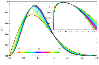
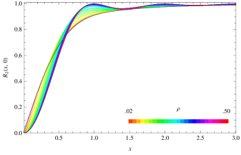
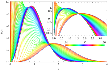
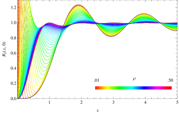
Figure 1: Level spacing distribution $P(s)$ and two-level correlation function $R_{2}(x,0)$ for GOE-GUE crossover. The $\rho$ parameter ranges $0.02\leq\rho\leq 0.70$ or $0.50$ by step 0.02. The two bounding curves correspond to the GOE and GUE limits, $\rho=0$ and $\infty$.

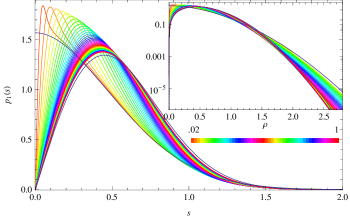
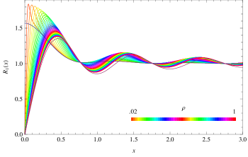
Figure 2: Level spacing distribution $P(s)$ and two-level correlation function $R_{2}(x,0)$ for GSE-GUE crossover. The $\rho$ parameter ranges and $0.01\leq\rho\leq 0.70$ or $0.50$ by step 0.01. The two bounding curves correspond to the GSE and GUE limits, $\rho=0$ and $\infty$.

Figure 3: Smallest eigenvalue distribution $p_{1}(s)$ and microscopic level density $R_{1}(x)$ for chGOE-chGUE crossover. The $\rho$ parameter ranges $0.02\leq\rho\leq 1.00$ by step 0.02. The two bounding curves correspond to the chGOE and chGUE limits, $\rho=0$ and $\infty$.

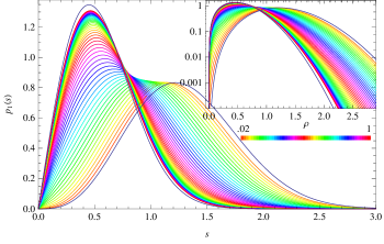
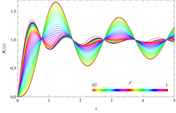
Figure 4: Smallest eigenvalue distribution $p_{1}(s)$ and microscopic level density $R_{1}(x)$ for chGSE-chGUE crossover. The $\rho$ parameter ranges $0.02\leq\rho\leq 1.00$ by step 0.02. The two bounding curves correspond to the chGSE and chGUE limits, $\rho=0$ and $\infty$.

We immediately observe the asymptotic behaviors of $P(s)$ and $p_{1}(s)$ for parametric (chiral) random matrices at finite $\rho$,

$$P^{(\rho)}(s)\sim C_{\rho}s^{2},\ \ p^{(\rho)}_{1}(s)\sim c_{\rho}s^{1}\ \ (s\ll 1);\ \ \ \ \log P^{(\rho)}(s),\ \log p_{1}^{(\rho)}(s)\sim-\gamma_{\rho}s^{2}\ \ (s\gg 1).$$ (12)

Here $C_{\rho},c_{\rho},\gamma_{\rho}$ are $\rho$-dependent constants, monotonically varying in $\rho$, in ranges $\pi^{2}/3<C_{\rho}<\infty$, ${\pi^{2}}/{2}<c_{\rho}<\infty$, ${\pi^{2}}/{16}<\gamma_{\rho}<{\pi^{2}}/{8}$, i.e., in between the (ch)GUE and the (ch)G(O,S)E limits.

For a bookkeeping purpose, we exhibit plots of the two-level correlation function $R_{2}(x,0)$ for nonchiral cases (3) in Figs. 1 and 2 (right) and the single-level density $R_{1}(x)$ for chiral cases in Figs. 3 and 4 (right). Note that the first peaks of $R_{2}(x,0)$ and $R_{1}(x)$ (right figures) are comprised of the corresponding $P(s)$ and $p_{1}(s)$ (left figures), respectively. In the subsequent section, these analytic results will be tested to fit the Dirac eigenvalue data numerically obtained from modified SU(2) lattice gauge models. The practical advantage of adopting distributions of individual level spacings [$P(s)$ and $p_{1}(s)$] over $n$-level correlation functions [$R_{2}(x,0)$ and $R_{1}(x)$] for fitting is clear from the figures. As the oscillation of the latter consists of overlapping of multiple peaks, the characteristic shape of each peak is inevitably smoothed out, leaving us with a rather structureless curve for which an accurate fit is difficult. On the other hand, the former and its cousins $p_{k}(s)$ (the distribution of the $k^{\rm th}$ smallest eigenvalue damn )

$$p_{k}(s)=-\frac{d}{ds}\left.\frac{1}{(k-1)!}\left(-\frac{\partial}{\partial z}\right)^{k-1}\sqrt{{\rm Det}(\openone-z\hat{K}_{s})}\right|_{z=1}$$ (13)

that could as well be computed by the Nyström-type method are very sensitive to the value of the crossover parameter, because Eqs. (11), (12) imply that the ratio of $P(s)$ or $p_{1}(s)$ for the orthogonal and sympletic classes to that for the unitary class grows as $\exp\frac{\pi^{2}s^{2}}{16}$ for large $s$ (it exceeds $10$ at $s\simeq 2$, $10^{2}$ at $s\simeq 2.7$, and $10^{4}$ at $s\simeq 4$). Therefore $P^{(\rho)}(s)$ and $p^{(\rho)}_{1}(s)$ should in principle admit very sharp one-parameter fitting by the least square method or simply from the tail of the curve (in the range of $s$ where the systematic deviation due to finite size is not prominent), as done for the Anderson tight-binding Hamiltonians at the metal-insulator transition shk versus the critical random matrix ensembles interpolating G(O,U,S)E and Poisson statistics nis . In the chGSE-chGUE case, the microscopic level density $R_{1}(x)$ [Fig. 4(b)] would also be suited for fitting, due to its characteristic oscillatory behavior for a wide range of $x$.

III Dirac Spectrum

III.1 Antiunitary symmetry

Dirac operator for the “real” QCD, i.e., for quark fields belonging to the real or pseudoreal representation of the gauge group, is known to possess a particular antiunitary symmetry unlike that for the complex representation ver . Namely, Euclidean Dirac operator $D=\gamma_{\mu}(i\partial_{\mu}+A_{\mu}^{a}\tau_{a})$ for quarks in the fundamental representation of SU(2) commutes with $C\tau_{2}K$. Here, $C$ is the charge conjugation matrix satisfying $C\gamma_{\mu}C^{-1}=-\gamma^{\ast}_{\mu}$, $\tau_{2}$ is one of the generators of the SU(2) gauge group satisfying $\tau_{2}\tau_{a}\tau_{2}^{-1}=-\tau_{a}^{\ast}$, and $K$ denotes the complex conjugation. As $(C\tau_{2}K)^{2}=+1$, $D$ can be brought to a real symmetric matrix by a similarity transformation. Similarly, the Dirac operator for quarks in the adjoint representation of SU($N$) commutes with $CK$. As $(CK)^{2}=-1$, $D$ can be brought to a quaternion self-dual matrix. By the same token, Dirac operators in fundamental representations of O($N$) and Sp(2$N$) gauge groups are real symmetric and quaternion self-dual, respectively. It is also well known that the reality and the self-duality of the continuum Dirac operators are interchanged for the corresponding Kogut-Susskind staggered Dirac operators [(17) below], i.e., $D^{\rm KS}$ in SU(2) fundamental is essentially quaternion self-dual, whereas $D^{\rm KS}$ in SU($N$) adjoint is real symmetric, due to the the absence of the charge conjugation matrix hv . The spectrum of the SU(2) fundamental staggered Dirac operator was indeed numerically shown to belong to the chGSE class bjmsvw .

Since the Dirac operator in the fundamental representation of U(1) (or SU($N^{\prime}\geq 3$) if one prefers) in continuum or on a lattice possesses no such antiunitary symmetry, the Dirac operator in the SU(2) fundamental (SU($N$) adjoint)$\times$U(1),

$$D=\gamma_{\mu}(i\partial_{\mu}+A_{\mu}^{a}T_{a}+B_{\mu}),$$ (14)

where $T_{a}$’s are the generators of the corresponding representation of SU(2) or SU($N$), and $B_{\mu}$ the $U(1)$ gauge field, either weakly fluctuating or fixed as a background, is endowed with a weakly broken antiunitary symmetry as compared to the pure SU(2) fundamental or SU($N$)-adjoint case.

III.2 Modified SU(2) lattice gauge theory

In contrast to the parametric random matrices $H=H_{\rm S}+i\alpha H_{\rm A}$ for which the breaking of the antiunitary symmetry is uniquely parametrized by ${\displaystyle\alpha=\sqrt{{\left\langle||{\rm Im}\,H||^{2}\right\rangle}/{\left\langle||{\rm Re}\,H||^{2}\right\rangle}}}$, it is not straightforward to identify the bare U(1) gauge coupling constant as proportional to $\alpha$, due to the gauge invariance: a Dirac operator that appears complex could actually be a U(1) gauge transform of some purely real matrix. In that case, its spectral fluctuation would perfectly be described by chGOE or chGSE. Thus, in this paper, we restrict ourselves to simpler models without such a subtlety: SU(2) quenched lattice gauge theory associated with twisted boundary condition or coupled with U(1) noise, each of which does contain an unambiguous counterpart of the $\alpha$ parameter.

We consider SU(2) quenched lattice gauge theory under the twisted boundary condition (TBC), that is to multiply SU(2) links variable at the temporal boundary of the hypercubic lattice of size $V=L^{4}$ by a constant phase

$${\rm e}^{i\theta_{n,\mu}}=\left\{\begin{array}[]{ll}{\rm e}^{i2\pi\varphi}&(n_{4}=L,\ \mu=4)\\ 1&(\mbox{else})\end{array}\right.,$$ (15)

with $\varphi\ll 1$. This twisting is gauge equivalent to the fixed vector U(1) background $B_{\mu}=({2\pi\varphi}/{L})\delta_{\mu,4}$ of AB flux $2\pi\varphi$ dm or the imaginary chemical potential $\mu={i2\pi\varphi}/{L}$. The flux $\varphi$ is the measure of antiunitary-symmetry violation and plays the role of $\alpha$ in the parametric random matrices. Its effect on the low-energy effective Lagrangian is completely dictated through the flavor-covariant derivative svd , just as in the case of symmetry-violating real chemical potentials kogut .

We also consider the SU(2) + U(1) phase noise (PhN) model, where an independent and identically distributeds random phase ${\rm e}^{i\theta_{n,\mu}}$ taken from the uniform distribution $\theta\in[-p,p]\ (p\ll 1)$ (one could alternatively adopt Gaussian distribution of variance $p^{2}$) is multiplied to each link SU(2) variable. The parameter $p$ of randomness is expected to be proportional to $\alpha$ in the parametric random matrices, since

$${\frac{\left\langle||{\rm Im}\,D||^{2}\right\rangle}{\left\langle||{\rm Re}\,D||^{2}\right\rangle}}\simeq{\frac{\left\langle||U\sin\theta||^{2}\right\rangle}{\left\langle||U\cos\theta||^{2}\right\rangle}}\simeq\left\langle\theta^{2}\right\rangle=\frac{1}{3}p^{2}.$$ (16)

The PhN model was previously used to uncover the fake nature sw of the apparent chGUE-chGSE crossover of the Dirac spectrum of Ginsparg-Wilson type fhlw , so it would be a good exercise to exploit it again to our actual universality crossover.

For our purpose of confirming that the lattice model exhibits chG(S,O)E-chGUE crossover, it is sufficient to focus on the strong coupling region of SU(2) at $\beta=4/g^{2}=0\sim 1.5$, where the smoothed level density at the origin, $1/\varDelta(0)$, is sufficiently above zero and the chiral symmetry is spontaneously broken, accepting that the model is away from the continuum limit. Accordingly, we employ the simplest algorithm possible: the unimproved plaquette action and the 10-hit heat-bath update coupled with overrelaxation. The staggered Dirac operator

$$D^{\rm KS}_{nm}=\frac{1}{2}\left(\eta_{n,\mu}\delta_{n+\hat{\mu},m}U_{n,\mu}{\rm e}^{i\theta_{n,\mu}}-\eta_{m,\mu}\delta_{n,m+\hat{\mu}}U_{m,\mu}^{\dagger}{\rm e}^{-i\theta_{m,\mu}}\right),\ \ \eta_{n,\mu}\equiv(-1)^{n_{1}+\ldots+n_{\mu-1}}$$ (17)

is diagonalized using the standard LA package.

Because of our need to detect possibly small deviations of spectral fluctuation from the universal random matrix statistics at either end ($\rho=0$ or $\infty$), we give priority to the number of independent samples and perform our simulation on a lattice of the smallest size $V=4^{4}$. This choice is sufficient for measuring the short-distance behavior of eigenvalues within up to 3$\sim$4 mean level spacings and determining the $\rho$ parameter precisely. In this region the systematic deviation due to the small size of the lattice is less prominent (they shall manifest at larger separation) than the statistical fluctuation. Only if one dares to test the symmetry crossover on the large-distance correlation of eigenvalues, such as the number variance $\Sigma^{2}(s)$, would the use of larger lattices become essential.

III.3 Fitting Dirac spectra

Our procedure of fitting Dirac spectral statistics to the parametric random matrix predictions consists of the following steps:

1. Determination of $\varDelta(0)$. Perform the pure SU(2) simulation for each $\beta$ and measure the fundamental and adjoint staggered Dirac spectrum $\{\lambda_{i}\}$ for $O(10^{5})$ configurations. Taking for granted that the small Dirac eigenvalues obey the chG(S,O)E statistics, determine the mean level spacing at the origin $\varDelta(0)$ in the following two ways:
   (a) Using the least square method, fit the histogram of the smallest Dirac eigenvalues $\wp_{1}(\lambda_{1})$ to the rescaled chG(S,O)E result (11), $p_{1}(\lambda_{1}/\varDelta)/\varDelta$, by varying $\varDelta$. The fitting range is chosen to be within $3\varDelta$ (chGSE) and $2.2\varDelta$ (chGOE), which is divided into bins of widths $0.1\varDelta$. Errors of $\varDelta$ are estimated as those increase $\chi^{2}$ by 1.
   (b) Compare the mean value of the smallest Dirac eigenvalue $\left\langle\lambda_{1}\right\rangle$ with that of the (unfolded) chiral random matrix eigenvalues from (11),

   $$\left\langle x_{1}\right\rangle=\int_{0}^{\infty}s\,p_{1}(s)ds=\sqrt{\frac{2{\rm e}}{\pi}}{\rm erfc}\frac{1}{\sqrt{2}}~{}~{}\mbox{[chGOE]},\ \ \sqrt{\frac{2{\rm e}}{\pi}}~{}~{}\mbox{[chGSE]}\ \ \Rightarrow\ \ \varDelta(0)=\frac{\left\langle\lambda_{1}\right\rangle}{\left\langle x_{1}\right\rangle}.$$ (18)

   Typically, the values of mean level spacing determined by the above two methods agree within $0.1\%$. This provides a ground for a precise determination of the crossover parameter at the origin in step 2.

2. Fitting the smallest eigenvalue. Multiply SU(2) link variables $U_{n,\mu}$ by the phases ${\rm e}^{i\theta_{n,\mu}}$ (either TBC or PhN) and measure the Dirac spectrum $\{\lambda_{i}\}$ for $N_{{\rm conf}}=O(10^{4})$ independent configurations. The unfolded smallest eigenvalue is still defined by $x_{1}=\lambda_{1}/\varDelta(0)$ with respect to $\varDelta(0)$ determined in step 1, i.e. from unmodified SU(2) configurations. Fit the frequencies of $x_{1}$ to the prediction by the least square method as follows: we choose the valid range of fitting the smallest eigenvalue $x_{1}$ to be [0, 2.8] (fundamental) and [0, 1.6] (adjoint) and divide them into $r=20$ segments ${I_{0},\ldots,I_{r-1}}$ of equal width. The remainder is denoted by $I_{r}=[$2.8 or 1.6, $\infty)$. Define ${\chi_{\rho}^{2}=\sum_{i=0}^{r}{(F_{i}-f_{i}^{(\rho)})^{2}}/{f_{i}^{(\rho)}},}$ where $F_{i}$ denotes the frequency of $x_{1}$ falling on the $i$th interval $I_{i}$, and $f_{i}^{(\rho)}=N_{{\rm conf}}\int_{I_{i}}p_{1}^{(\rho)}(s)ds$ its expected value from the chG(S,O)E-chGUE parametric random matrices. By varying $\rho$, find the optimal value of $\rho$ that minimizes $\chi^{2}_{\rho}$ and estimate the error of $\rho$ as that increases $\chi^{2}_{\rho}$ by 1.

3. Fitting level spacings. Fluctuation of Dirac eigenvalues in the spectral bulk is, by itself, not directly related to the low-energy effective description of the gauge theory but rather to the diffusion of quarks in a hypothetical “time” evolution with Dirac operator as its Hamiltonian jnpz2 . Nevertheless, we shall argue that the distribution of level spacings from the spectral “plateaux” $[\lambda_{\rm m},\lambda_{\rm M}]$ adjacent to, but not including, the origin, in which the mean level spacing $\varDelta(\lambda)$ is well approximated as a constant close to $\varDelta(0)$ (Fig.5), provides an efficient way of determining $F$. It also serves as a clearer indicator of the presence of the universality crossover in modified SU(2) lattice gauge theories and as a consistency check of the $\rho$ value directly measured from the smallest eigenvalues distribution. In order to avoid possible distortion of the level spacing distribution due to the chiralness, we take $\lambda_{\rm m}$ not too close to the origin and set it to be, at smallest, the $11^{\rm th}$ eigenvalue.
   Define unfolded level spacings in that eigenvalue window as $s=(\lambda_{i+1}-\lambda_{i})/\varDelta(\bar{\lambda}),\ \lambda_{i},\lambda_{i+1}\in[\lambda_{\rm m},\lambda_{\rm M}]$. In case the density profile near the origin is not quite flat (such as $D^{\rm KS}$ in SU(2) fundamental at $\beta=0.5\sim 1.5$), we alternatively used unfolding by the linearized level density $\bar{\rho}(\lambda)$, $\lambda_{i}\to x_{i}=\int^{\lambda_{i}}\bar{\rho}(\lambda)d\lambda,$ even within the window chosen, to offset the explicit local variation in the mean level spacing. For a window containing $\sim 20$ eigenvalues, the distortion in $P_{\rm data}(s)$ caused by the small local inhomogeneity of the $\rho$ parameter through its dependence on $\varDelta=1/\bar{\rho}$ is expected to be negligible. Find the best fit of the histogram of the unfolded smallest Dirac eigenvalues $P_{\rm data}(s)$ to the crossover chiral random matrix result $P^{(\rho)}(s)$ [Figs. 2(a) or 1(a)] by varying $\rho$, as done in step 2. Thanks to the enormous gain in statistics due to the spectral averaging, we can safely set the fitting range to be as large as [0, 4] and divide it into $r=40$ segments.

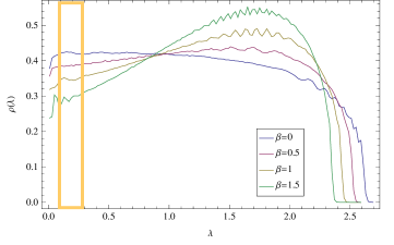
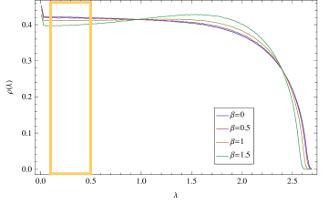
Figure 5: Macroscopic level densities $\rho(\lambda)$ of SU(2) fundamental (left) and adjoint (right) $D^{\rm KS}$ at various $\beta$ in the strong coupling region. Lattice size: $4^{4}$, number of configurations: $100,000$. Level spacings from the eigenvalue windows (plateaux) $[\lambda_{\rm m},\lambda_{\rm M}]$ marked by orange strips in the vicinity of $\lambda=0$ are used for fitting $P^{(\rho)}(s)$.

III.4 Simulation results

We present the outcome of one-parameter fitting of smallest eigenvalue distributions (SED) and level spacing distributions (LSD) to the parametric random matrix ensembles. We set the symmetry-breaking parameters to be $\varphi=0.01\sim.06$ for the SU(2)+TBC model and $p=0.02\sim.10$ for the SU(2)+PhN model and performed simulations at the gauge-coupling constants $\beta=0,0.5,1,1.5$ on a lattice of dimensions $V=4^{4}$. $N_{\rm conf}=40,000$ configurations are generated for each set of parameters. Optimal values of the $\rho$ parameter for the TBC (PhN) model in fundamental (F) and adjoint (A) representation are tabulated in the six (seven) columns in the middle of Table I (II).

Sample plots of $p_{1}(s)$, $R_{1}(x)$, and $P(s)$ for $\beta=0$ are exhibited in Figs.6$\sim$8 [SU(2)+TBC] and in Figs.9$\sim$11 [SU(2)+PhN]. In all figures, measured histograms are plotted by colored dots, and parametric random matrix results that fit the data optimally are shown in curves of the same color ($\varphi=.01$ or $p=.02$ in red to $\varphi=.06$ or $p=.10$ in green). Also plotted in the figures are the results from chG(S,O)E or G(S,O)E (black real line), and chGUE or GUE (broken line). Note that the microscopic level density $R_{1}(x)$ is not fitted to the corresponding data by the least square method; the $\rho$ parameter determined from the SED is adopted to the respective $R_{1}(x)$.

Even at inspection, one is convinced of the accuracy of one-parameter fitting in all cases. The $\chi^{2}$/d.o.f. deviations from optimally fitting random matrix distributions are summarized in Table III. Considering the smallness of our lattice ($4^{4}$), the goodness-of-fit achieved is astonishing (except for LSDs for SU(2) fundamental at very small $\rho\lesssim 0.1$, where the distribution becomes extremely peaky at small $s$ due to the onset of Kramers degeneracy and the fitting error is inevitably enhanced). These listed values are comparable to those reported in the pioneering papers in this field dam1 using chGUE-chGUE (i.e. Hermitian) crossover, fitted to the spectral data from larger lattices: $\chi^{2}$/d.o.f.$=0.33$ for quenched QCD on $12^{4}$ and $\chi^{2}$/d.o.f.$=1.13\sim 1.33$ for dynamical QCD on $6^{4}$.

From Tables I and II one immediately notices that for a fixed bare coupling $\beta$, $\varphi$-$\rho$ and $p$-$\rho$ plots are all quite linear. In Fig. 12 we exhibit sample plots of ${\sqrt{\varDelta}}\rho/\varphi$ for SU(2)+TBC and ${\sqrt{\varDelta}}\rho/p$ for SU(2)+PhN , showing that (i) these ratios, namely from LSDs, are very stable under the change of symmetry-violating parameters $\varphi$ or $p$ and (ii) the values of $\rho$ determined from SED and from LSD are in a good agreement, as should be. This precisely linear dependence is essential in accurately determining the pion decay constant from SU(2)+TBC models in the next section. We note that in the strong coupling limit $\beta=0$, four plots nearly overlap on top of each other, regardless of the representation being fundamental (F) or adjoint (A) (see also Fig. 13). The splitting between fundamental and adjoint becomes more apparent at larger value of $\beta$.

Table 1: SU(2) + TBC model on $V=4^{4}$: Crossover parameters and low-energy constants

$\beta$	rep/dist		$\varDelta$	$\Sigma$	$\rho$						$\sqrt{\varDelta}\rho/\mu$	$F^{2}/\Sigma$	$F^{2}$
		$[\lambda_{\rm m},\lambda_{\rm M}]$			$\varphi$=.01	.02	.03	.04	.05	.06
0	F/SED		.00933(1)	1.315(2)	.061(1)	.123(1)	.181(1)	.245(2)	.305(2)	.364(2)	.375(1)	.221(1)	.290(2)
	F/LSD	[.10, .30]	.00929(0)	1.321(0)	.061(0)	.122(0)	.183(1)	.243(1)	.303(2)	.364(4)	.374(1)	.219(1)	.290(1)
	A/SED		.00617(0)	1.989(1)	.076(1)	.153(2)	.224(3)	.309(5)	.391(8)	.453(11)	.382(2)	.229(3)	.455(6)
	A/LSD	[.10, .50]	.00618(0)	1.984(0)	.075(2)	.150(4)	.224(6)	.297(8)	.371(14)	.447(25)	.374(5)	.219(5)	.435(11)
0.5	F/SED		.01020(1)	1.203(2)	.055(1)	.110(1)	.160(1)	.210(2)	.263(2)	.313(2)	.339(1)	.180(1)	.217(1)
	F/LSD	[.10, .26]	.01004(0)	1.223(0)	.052(0)	.103(0)	.155(1)	.206(1)	.257(2)	.306(2)	.329(1)	.170(1)	.208(1)
	A/SED		.00626(2)	1.960(6)	.067(1)	.131(2)	.200(3)	.263(4)	.327(6)	.386(8)	.332(2)	.173(2)	.339(5)
	A/LSD	[.10, .50]	.00622(0)	1.972(0)	.067(3)	.134(4)	.202(5)	.269(7)	.333(11)	.407(17)	.337(4)	.179(5)	.353(9)
1.0	F/SED		.01150(5)	1.067(5)	.056(1)	.102(1)	.148(1)	.193(1)	.241(2)	.286(2)	.329(1)	.170(1)	.181(1)
	F/LSD	[.10, .30]	.01105(0)	1.110(0)	.048(0)	.095(0)	.143(1)	.190(1)	.237(1)	.284(2)	.319(1)	.160(1)	.177(1)
	A/SED		.00631(3)	1.944(9)	.065(1)	.132(2)	.200(3)	.266(4)	.338(6)	.397(8)	.336(2)	.177(2)	.344(5)
	A/LSD	[.10, .50]	.00632(0)	1.943(0)	.066(3)	.133(4)	.199(5)	.266(7)	.331(10)	.394(16)	.335(4)	.176(4)	.343(9)
1.5	F/SED		.01412(1)	0.869(0)	.061(1)	.101(2)	.138(1)	.178(1)	.218(2)	.257(2)	.329(1)	.170(1)	.148(1)
	F/LSD	[.13, .28]	.01280(0)	0.959(0)	.043(0)	.085(0)	.127(1)	.169(1)	.210(1)	.251(1)	.319(1)	.160(1)	.153(1)
	A/SED		.00654(1)	1.877(3)	.067(1)	.128(2)	.193(3)	.251(4)	.312(6)	.392(8)	.336(2)	.177(2)	.333(5)
	A/LSD	[.10, .50]	.00650(0)	1.887(0)	.065(3)	.128(4)	.194(5)	.257(7)	.322(10)	.386(15)	.335(4)	.176(4)	.333(8)

Table 2: SU(2) + PhN model on $V=4^{4}$: Crossover parameters

$\beta$	rep/dist		$\varDelta$	$\rho$							$\sqrt{\varDelta}\rho/p$
		$[\lambda_{\rm m},\lambda_{\rm M}]$		$p$=.02	.03	.04	.05	.06	.08	.10
0	F/SED		.00933(1)	.079(1)	.117(1)	.154(1)	.194(1)	.235(2)	.311(2)	.390(1)	.376(0)
	F/LSD	[.10, .30]	.00929(0)	.078(0)	.117(0)	.156(1)	.194(1)	.233(1)	.311(2)	.387(3)	.375(0)
	A/SED		.00617(0)	.094(2)	.145(2)	.193(3)	.244(4)	.288(5)	.381(8)	.481(7)	.377(2)
	A/LSD	[.10, .50]	.00618(0)	.095(3)	.142(4)	.191(5)	.237(6)	.285(8)	.383(15)	.471(18)	.374(4)
0.5	F/SED		.01020(1)	.071(1)	.106(1)	.143(1)	.178(1)	.213(1)	.286(1)	.353(2)	.360(0)
	F/LSD	[.10, .26]	.01009(0)	.072(0)	.108(0)	.143(1)	.179(1)	.215(1)	.286(1)	.359(4)	.361(0)
	A/SED		.00626(2)	.094(2)	.140(2)	.185(3)	.230(4)	.274(4)	.367(5)	.446(10)	.365(2)
	A/LSD	[.10, .50]	.00622(0)	.094(3)	.142(4)	.189(5)	.235(6)	.283(8)	.377(10)	.468(28)	.372(4)
1.0	F/SED		.01150(5)	.062(1)	.094(1)	.125(1)	.156(1)	.188(1)	.255(2)	.316(2)	.338(0)
	F/LSD	[.10, .30]	.01120(0)	.065(0)	.097(0)	.130(0)	.162(1)	.194(1)	.259(2)	.322(3)	.343(0)
	A/SED		.00631(3)	.092(2)	.140(2)	.188(3)	.233(4)	.286(5)	.376(7)	.490(12)	.373(2)
	A/LSD	[.10, .50]	.00632(0)	.094(3)	.138(4)	.186(5)	.231(6)	.280(8)	.374(14)	.459(27)	.369(4)

Table 3: $\chi^{2}/$d.o.f. for fitting spectral distributions

dist	rep	SU(2)+TBC				SU(2)+PhN
		$\beta$=0	0.5	1.0	1.5	$\beta$=0	0.5	1.0
SED	F	0.79$\sim$1.22	0.54$\sim$1.00	0.64$\sim$1.80	0.86$\sim$3.13	0.58$\sim$1.33	0.63$\sim$1.50	0.73$\sim$1.44
	A	0.61$\sim$1.11	0.36$\sim$1.24	0.80$\sim$1.59	0.79$\sim$1.31	0.41$\sim$1.42	0.65$\sim$1.88	0.60$\sim$1.49
LSD	F*	0.65$\sim$1.07	1.11$\sim$1.53	0.63$\sim$1.61	0.89$\sim$1.41	0.61$\sim$1.54	0.55$\sim$1.29	0.78$\sim$1.71
	A	0.97$\sim$1.55	0.63$\sim$1.09	0.57$\sim$1.15	0.60$\sim$1.17	0.61$\sim$1.40	0.80$\sim$1.22	0.72$\sim$1.21

$*$ excludes F/LSD for TBC at $\rho\lesssim 0.1$, for which $\chi^{2}/$d.o.f.=$3\sim 5$.

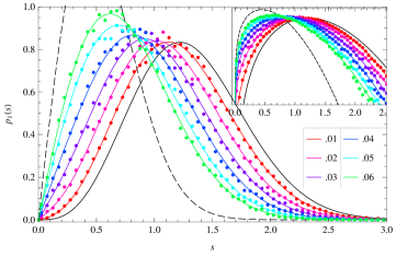
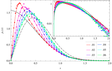
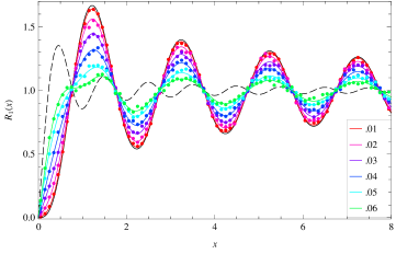
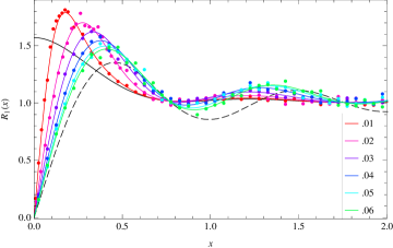
Figure 6: Smallest eigenvalue distributions of SU(2)+TBC $D^{\rm KS}$ in fundamental (left) and adjoint (right), at $\beta=0$ and $\varphi=0.01\sim.06$.

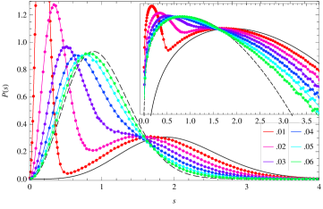
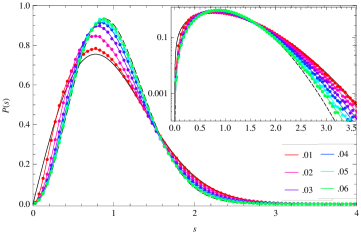
Figure 7: Microscopic level densities of SU(2)+TBC $D^{\rm KS}$ in fundamental (left) and adjoint (right), at $\beta=0$ and $\varphi=0.01\sim.06$.

Figure 8: Level spacing distributions of SU(2)+TBC $D^{\rm KS}$ in fundamental (left) and adjoint (right), at $\beta=0$ and $\varphi=0.01\sim.06$.

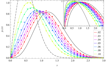
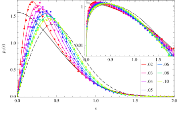
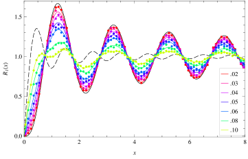
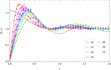
Figure 9: Smallest eigenvalue distributions of SU(2)+PhN $D^{\rm KS}$ in fundamental (left) and adjoint (right), at $\beta=0$ and $p=0.02\sim.10$.

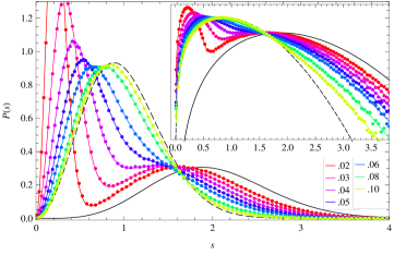
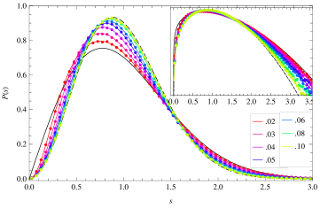
Figure 10: Microscopic level densities of SU(2)+PhN $D^{\rm KS}$ in fundamental (left) and adjoint (right), at $\beta=0$ and $p=0.02\sim.10$.

Figure 11: Level spacing distributions of SU(2)+PhN $D^{\rm KS}$ in fundamental (left) and adjoint (right), at $\beta=0$ and $\varphi=0.02\sim.10$.

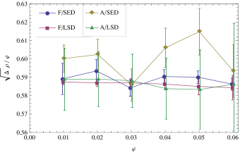
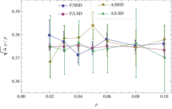
Figure 12: The ratio between the symmetry-violating parameters $\varphi$ and $p$ versus the crossover parameter $\sqrt{\varDelta}\rho$ for SU(2)+TBC model (left) and SU(2) + PhN model (right) in the strong coupling limit $\beta=0$, as tabulated in Table I and II.

IV Low-Energy Constants

IV.1 Chiral Lagrangian

Below, we briefly review the chiral Lagrangian description of QCD-like theories and sketch the identification of the low-energy constants with the parameters of random matrices. The effective low-energy Lagrangian for QCD-like theories with $N_{F}$ flavors of quarks in (pseudo-)real representation, at finite chemical potential $\mu$ and bare quark mass $m$ is unambiguously fixed by the global symmetry alone (provided that $\mu$ is much smaller than the $\rho$ meson mass) and takes the form containing two phenomenological free parameters $F$ and $\Sigma$ kogut ,

$${\cal L}_{\rm eff}(Q)=\frac{1}{2}F^{2}\,{\rm tr}\,\partial_{\mu}Q^{\dagger}\partial_{\mu}Q+2F^{2}\mu\,{\rm tr}\,\hat{B}Q^{\dagger}\partial_{0}Q-F^{2}\mu^{2}\,{\rm tr}\,(\hat{B}Q^{\dagger}\hat{B}Q+\hat{B}\hat{B})-\frac{1}{2}\Sigma m\,{\rm Re}\,{\rm tr}\,\hat{M}Q.$$ (19)

Here $Q(x)$ is an SU($2N_{F}$) matrix-valued Nambu-Goldstone field, $\hat{B}=\sigma_{3}\otimes\openone_{N_{F}}$, $\hat{M}=\sigma_{1}\otimes\openone_{N_{F}}$ $\left(i\sigma_{2}\otimes\openone_{N_{F}}\right)$ for quarks in a real (pseudoreal) representation. $F$ is the “pion” decay constant and $\Sigma=\left\langle\bar{\psi}\psi\right\rangle/N_{F}$ the chiral condensate, both measured in the chiral and zero-chemical potential limit $m,\,\mu\to 0$. If the theory is in a finite volume $V=L^{4}$ and Thouless energy defined as ${E_{c}\simeq{F^{2}}/{\Sigma L^{2}}}$ is much larger than $m$, the path integral is dominated by the zero-mode integration

$$Z=\int_{{\rm SU}(2N_{F})}\!\!\!\!\!\!\!\!\!\!\!\!\!dQ\,\,\,\exp\left(V\mu^{2}F^{2}\,{\rm tr}\,(\hat{B}Q^{\dagger}\hat{B}Q+\hat{B}\hat{B})+\frac{1}{2}V\Sigma m\,{\rm Re}\,{\rm tr}\,\hat{M}Q\right),$$ (20)

and the theory is said to be in the $\varepsilon$ regime. In order to extract the Dirac spectrum, one introduces fictitious bosonic quarks as well as fermionic quarks in the fundamental theory, leading to the graded group version of (20) on the effective theory side. For the actual computation, one needs to parametrize the graded matrix $Q$ in terms of its eigenvalues. Comparing the resulting expression (after analytic continuation $\mu\to i\mu$ and $m\to i\lambda$) with the random matrix results (8) and (9), the coefficients of chemical-potential and “mass” terms in the exponents on both sides are readily identified as $4VF^{2}\mu^{2}=2\pi^{2}\rho^{2}$ and $V\Sigma\lambda=\pi x.$ The latter is merely the definition of unfolded eigenvalues $x=\lambda/\varDelta$, when combined with Banks-Casher relation $\Sigma=\pi/\varDelta V$ that determines one of the low-energy constants $\Sigma$ in terms of the mean spacing $\varDelta$ of small Dirac eigenvalues. Eliminating the volume in favor of the level spacing, the former equation reads

$${\sqrt{\varDelta}}\,\rho=\sqrt{\frac{2}{\pi}\frac{F^{2}}{\Sigma}}\mu,$$ (21)

where the left-hand side is a volume-independent combination. Accordingly, one can determine another low-energy constant $F^{2}/\Sigma$ from the slope of $\mu$-${\sqrt{\varDelta}}\rho$ plots, preferably on lattices of various sizes. Note that in the parameter region $V\Sigma|m|\gg 1$, Eq.(20) should approach the $\sigma$ model of nonchiral parametric random matrix ensembles aie , but we see no reason why the “pion decay” or diffusion constant multiplying ${\rm tr}\,\hat{B}Q^{\dagger}\hat{B}Q$ is affected. Accordingly, if the mean level spacing is approximately constant in a window in the very vicinity of the origin, one can determine $F^{2}/\Sigma$ from the bulk correlation (namely the LSD) in that window.

IV.2 SU(2) + twisted BC

As the imaginary chemical potential is equal to the flux per link, $\mu=(2\pi/L)\varphi$, $F^{2}/\Sigma$ can be extracted from the $\varphi$-${\sqrt{\varDelta}}\rho$ plots for the SU(2)+TBC model. In Table I we exhibit the values of $F^{2}/\Sigma$ determined from the slopes of these $\varphi$-${\sqrt{\varDelta}}\rho$ plots, with all the numerals in the lattice unit. We also list the mean level spacings ($\varDelta(0)$ for the SED rows and $\varDelta([\lambda_{\rm m},\lambda_{\rm M}])$ for the LSD rows) and the chiral condensate $\Sigma$. The pion decay constant $F^{2}$ is then obtained by multiplying $F^{2}/\Sigma$ and $\Sigma$ in each row. Coupling dependence of these low-energy constants as determined from respective spectral distributions are summarized in Fig.13. In order to offset the number of components in the gauge multiplet, the constants for adjoint quarks are multiplied by 2/3 in the plot. We notice that except for the SU(2) fundamental at $\beta=0.5$ and 1.5, two values of $F^{2}$, one determined solely from the zero-virtuality correlations (SED) and the other from the bulk correlations (LSD), agree within the one-$\sigma$ error bars. Although it is admittedly difficult to calibrate the systematic deviations involved in employing the bulk correlation for the determination of $F$ (part of which could originate from nonzero modes of the effective theory or from the nonuniformity of the mean level spacing within the eigenvalue window (see Fig. 5, left) due to the smallness of the lattice), these numerical agreements could justify the latter method using LSDs a posteriori.

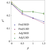
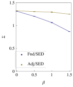
Figure 13: Low-energy constants $F^{2}$ and $\Sigma$ for SU(2) quenched lattice gauge theory. Values are multiplied by 2/3 for the adjoint.

At $\beta=0$, both low-energy constants agree between fundamental and adjoint representations. This observation is consistent with the fact that in the strong coupling limit the low-energy constants are identical to the Sp($N$) and O($N$) lattice gauge theories at large $N$ nn , which share the same antiunitary symmetries as SU(2) fundamental and adjoint. We also notice that due to the onset of chiral symmetry restoration at $\beta=1.5$, the microscopic level density $R_{1}(x)$ for SU(2) fundamental starts to deviate from the random matrix result at $x\gtrsim 2$ (Fig. 14, left). Thus the range of $x$ available for fitting the SED is rather limited, especially on a lattice as small as $V=4^{4}$. On the other hand, the LSDs near the origin, not being directly sensitive to the chiral symmetry, are still fittable to the random matrix result without noticeable deviation throughout the plotted region (Fig. 14, right), and the values of $\sqrt{\Delta}\rho$ determined from the LSD retain the linear dependence on $\varphi$. Therefore, we consider the fitting of LSDs to the parametric nonchiral random matrices to be an efficient method of extracting $F^{2}$ from small lattices.

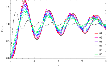
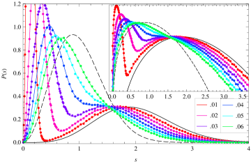
Figure 14: Microscopic level density (left) and level spacing distribution (right) of SU(2)+TBC $D^{\rm KS}$ in fundamental representation, at $\beta=1.5$ and $\varphi=0.01\sim.06$.

IV.3 SU(2) + phase noise

The strength of phase randomness $p$ in the SU(2)+PhN model is not related to the imaginary chemical potential and thus cannot be directly used to determine $F^{2}$ from the response of the Dirac spectra. Thus, we merely list in Table II the slopes of $p$-${\sqrt{\varDelta}}\rho$ plots as a counterpart of $\mu$-${\sqrt{\varDelta}}\rho$ plots. We, however, noticed, rather unexpectedly, that for the SU(2) theory at the strong coupling limit $\beta=0$, the “conversion ratio” between the phase randomness $p$ and the imaginary chemical potential $\mu$ is unity within numerical error (see the $\sqrt{\varDelta}\rho/\mu$ column in Table I and the $\sqrt{\varDelta}\rho/p$ column in Table II). This fact will have to be accounted for analytically. They gradually disagree for increasing $\beta$.

Finally, we need to check the volume dependence of the crossover parameter, which should scale as $\rho=(\sqrt{2}F\mu/\pi)\sqrt{V}$. Only for the purpose of varying the volume of the lattice in small steps, we adopted the two-dimensional toy model of SU(2)+PhN at $\beta=0$. $N_{\rm conf}=22,000$ independent configurations are generated for each set of parameters. First, we confirmed that the model shares the features in four dimensions, i.e., all spectral distributions fit nicely to the parametric random matrices, and $\sqrt{\Delta}\rho$ scales with the randomness $p$ on a lattice of fixed size $V=16^{2}$ (Fig.15). The eigenvalue windows for sampling levels spacings are chosen to be $[\lambda_{\rm m},\lambda_{\rm M}]=[0.30,0.65]$ (fundamental) and [0.16, 0.60] (adjoint). Then the $\rho$ parameter is measured from the level spacing distributions on lattices of size $V=10^{2}\sim 24^{2}$ at fixed phase randomness $p=0.03$. $\rho$ is indeed seen to scale as expected, linearly increasing in $\sqrt{V}$ (Fig.16).

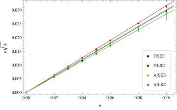
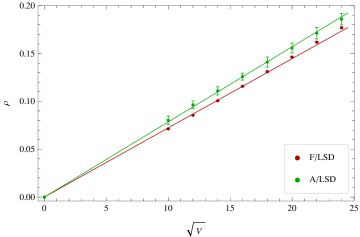
Figure 15: (left) Crossover parameter $\sqrt{\Delta}\rho$ for SU(2)+PhN model at $\beta=0$ and $p=0.02\sim.10$. Lattice size: $16^{2}$, number of configurations: $22000$. Eigenvalue windows: $[\lambda_{\rm m},\lambda_{\rm M}]=[0.30,0.65]$ (F), [0.16, 0.60] (A). Real lines are linear fits to the data.

Figure 16: (right) Volume dependence of the crossover parameter $\rho$ for SU(2)+PhN model at $\beta=0$ and $p=0.03$, determined from LSDs. Lattice size: $10^{2}\sim 24^{2}$. Other parameters are common to Fig.15.

V Conclusions

In this paper we have computed the level spacing and smallest eigenvalue distributions of Hermitian random matrices in the G(O,S)E-GUE and chG(O,S)E-chGUE crossover. The results are shown to be perfectly fittable to the adjoint and fundamental staggered Dirac spectra of quenched SU(2) lattice gauge theory whose antiunitary symmetry is weakly violated by twisted boundary condition or noisy phases. This leads to the precise determination of the pion decay constant $F$ (in the chiral and zero-density limit) from the Dirac spectral data. This method, feasible on a small-size lattice, has an advantage over the conventional method of measuring the decay rate of axial correlators, which requires a large temporal dimension.

Our treatment is complementary to the previous approach of determining $F$ of two-color QCD from its Dirac spectrum: Akemann and collaborators have concentrated on the real chemical potential, measured the response of Dirac eigenvalues that permeate into the complex plane, and fitted the lattice data to the non-Hermitian parametric chiral random matrices ake . On the other hand, we considered the twisted boundary condition, i.e., the imaginary chemical potential and measured the response of Dirac eigenvalues that cross over within the real axis, and fitted to the Hermitian parametric chiral random matrices. In terms of chiral Lagrangian, the difference is solely in the sign of $\mu^{2}$, and the integral formulas involving (original or modified) Bessel functions (8), (9) originated from the $\sigma$ model action are shared by the two. Similar complementary treatments were applied for three-color QCD at real and imaginary isospin chemical potential, which correspond to non-Hermitian chiral random matrices dam1 and Hermitian chiral random matrices in chGUE-chGUE crossover dam2 ; bw ; ai , respectively, resulting in a successful determination of $F$. Combined with the results reported in this paper filling the missing pieces, the fact that the Dirac spectral statistics in all three cases (SU(2) fundamental+$\mu$, SU(2) adjoint+$\mu$, SU(3) fundamental+$\mu_{\rm iso}$) agree perfectly with the predictions from corresponding identical zero-mode-approximated chiral Lagrangians in both regions of signs of $\mu^{2}$ constitutes a solid evidence for the validity of analytic continuation in the $\mu$ plane, which is much required for the actual physics, i.e., three-color QCD at real baryon number chemical potential.

We consider the use of imaginary chemical potential has a practical advantage for the following reason. In order to fit non-Hermitian Dirac spectra to the non-Hermitian random matrix result, one usually projects the complex eigenvalues either to the real or imaginary axis, and this projection could blur the fitting. Freer two-dimensional motion of complex eigenvalues is likely to lead to large statistical fluctuation. On the other hand, confining the eigenvalues within the real axis averts such issues, yielding a precise fitting shown in Figs.6$\sim$11.

Sharpness of the fitting functions chosen, $p_{1}(s)$ and $P(s)$, is also in our advantage. Note that the use of Wigner surmise (random $2\times 2$ matrices) of $p_{1}(s)$ and $P(s)$ for the parametric random matrices abps ; sbw is an uncontrolled approximation and is not suited for the precise determination of $F$, especially from fitting in the range of $s\gtrsim 2$ nis2012 . The advantage of our treatment is that exponentially fast, uniform convergence is guaranteed for Nyström-type method at increasing order.

Our next obvious step is to include weakly coupled QED in the simulation, rather than the phase noise treated in this paper. Our preliminary study shows that Dirac spectra of SU(2)$\times$U(1) quenched gauge theory are again fitted well to the parametric random matrix predictions, and we are currently accumulating numerical data on lattices of larger size than the current paper. This two-color QCD + QED model could be of interest to the lattice gauge community in which the three-color QCD + QED simulation in pursuit of precise measurement of isospin-related observables has attracted attention recently bdhiuyz , although we are exploiting the very difference of symmetry of SU(2)$\times$U(1) as compared to SU(3)$\times$U(1). Other possible extensions are the following:

1. In order to reduce the statistical error of fitting SEDs $p_{1}(s)$ for which the spectral averaging is not applicable, one could simultaneously use the $k^{\rm th}$ smallest eigenvalues distribution $p_{k}(s),k=2,3,\ldots$ [computable by Eq.(13)] alongside with $p_{1}(s)$ for fitting $\rho$ and look for the overlapping of their error bars.

2. Extension of our treatment to Dirac spectrum in a nontrivial SU(2) gauge field topology is straightforward: on the lattice side one should measure the overlap Dirac spectrum bw , whereas on the random matrix side the indices of the Bessel $J$ functions in Eqs.(8) and (9) are to be incremented by the topological charge $\nu$.

3. Introduction of dynamical quarks is interesting beyond the obvious reason of approaching more “realistic” models of QCD; the weakly symmetry-violating U(1) gauge randomness couples to the SU(2) gauge randomness through the quark loops (fermion determinant) only in that case. This correlation between perturbed and perturbing can possibly bring nontrivial distortion to the relationship between the bare U(1) coupling constant and the crossover parameter, i.e. the pion decay constant. Introduction of finite quark masses on the random matrix side could become cumbersome, but in the light of individual eigenvalue distributions for chGUE-chGUE crossover (the latter of Ref. dam2 ), the computation is still feasible.

4. Our result suggests a possibility of an exotic continuum limit, in which the rate of decoupling of U(1) gauge field is adjusted to the rate of approaching the thermodynamic limit, while keeping the $\mu^{2}F^{2}$ fixed. Albeit a rather artificial limit, this procedure might define a theory in which a nontrivial effect is induced to the interaction of Nambu-Goldstone bosons by the decoupling gauge interaction through the violation of antiunitary symmetry. The asymptotic slavery of U(1) is not an essential obstacle to this possibility, because any gauge field in the complex representation, namely the fundamental of SU($N^{\prime}\geq 3$), is equally suited as a pertinent perturbation violating the antiunitary symmetry of SU(2).

In forthcoming papers we wish to complete the project started here by covering up the directions listed above.

- (1) A. Nakamura, Phys. Lett. B 149, 391 (1984); See also for review: S. Muroya, A. Nakamura, C. Nonaka, and T. Takaishi, Prog. Theor. Phys. 110, 615 (2003).
- (2) M. E. Peskin, Nucl. Phys. B 175, 197 (1980).
- (3) H. Leutwyler and A. Smilga, Phys. Rev. D 46, 5607 (1992).
- (4) C. Vafa and E. Witten, Nucl. Phys. B 234, 173 (1984).
- (5) J. B. Kogut, M. A. Stephanov, and D. Toublan, Phys. Lett. B 464, 183 (1999).
- (6) J. B. Kogut, M. A. Stephanov, D. Toublan, J. J. M. Verbaarschot, and A. Zhitnitsky, Nucl. Phys. B 582, 477 (2000).
- (7) K. Splittorff, D. Toublan, and J. J. M. Verbaarschot, Nucl. Phys. B 620, 290 (2002); Nucl. Phys. B 639, 524 (2002).
- (8) G. V. Dunne and S. M. Nishigaki, Nucl. Phys. B 654, 445 (2003); Nucl. Phys. B 670, 307 (2003).
- (9) E. Dagotto, F. Karsch, and A. Moreo, Phys. Lett. B 169, 421 (1986).
- (10) C. Baillie, K. C. Bowler, P. E. Gibbs, I. M. Barbour, and M. Rafique, Phys. Lett. B 197, 195 (1987).
- (11) S. Hands, J. B. Kogut, M. P. Lombardo, and S. E. Morrison, Nucl. Phys. B 558, 327 (1999).
- (12) J. B. Kogut, D. Toublan and D. K. Sinclair, Nucl. Phys. B 642, 181 (2002).
- (13) J. J. M. Verbaarschot, Phys. Rev. Lett. 72, 2531 (1994).
- (14) F. J. Dyson, J. Math. Phys. 3, 1199 (1962).
- (15) E. V. Shuryak and J. J. M. Verbaarschot, Nucl. Phys. A 560, 306 (1993).
- (16) J. J. M. Verbaarschot and I. Zahed, Phys. Rev. Lett. 70, 3852 (1993).
- (17) M. A. Halasz, A.D. Jackson, and J. J. M. Verbaarschot, Phys. Rev. D 56, 5140 (1997); M. A. Halasz, J. C. Osborn, and J. J. M. Verbaarschot, Phys. Rev. D 56, 7059 (1997).
- (18) G. Akemann, E. Bittner, M.-P. Lombardo, H. Markum, and R. Pullirsch, Nucl. Phys. Proc. Suppl. 140, 568 (2005); G. Akemann and E. Bittner, Phys. Rev. Lett. 96, 222002 (2006); G. Akemann, Int. J. Mod. Phys. A 22, 1077 (2007); G. Akemann, T. Kanazawa, M. J. Phillips, and T. Wettig, J. High Energy Phys. 03, 066 (2011).
- (19) R. A. Janik, M. A. Nowak, G. Papp, and I. Zahed, Phys. Lett. B 440, 123 (1998); arXiv: hep-ph/9807499; Nucl. Phys. Proc. Suppl. 83, 977 (2000).
- (20) C. T. Sachrajda and G. Villadoro, Phys. Lett. B 609, 73 (2005).
- (21) T. Mehen and B. C. Tiburzi, Phys. Rev. D 72, 014501 (2005).
- (22) F. J. Dyson, J. Math. Phys. 3, 1191 (1962).
- (23) M. L. Mehta and A. Pandey, J. Phys. A: Math. Gen. 16, 2655 (1983); J. Phys. A: Math. Gen. 16, L601 (1983).
- (24) M. L. Mehta, Random Matrices, 3rd ed., (Elsevier, New York, 2004).
- (25) A. Altland, S. Iida, and K. B. Efetov, J. Phys. A: Math. Gen. 26, 3545 (1993).
- (26) A. V. Andreev, B. D. Simons, and B. L. Altsuler, J. Math. Phys. 37, 4968 (1996).
- (27) O. Bohigas, M.-J. Giannoni, A. M. O. de Almeida, and C. Schmit, Nonlinearity 8, 203 (1995).
- (28) K. Saito and T. Nagao, Phys. Lett. A 352, 380 (2006); T. Nagao, P. Braun, S. Müller, K. Saito, S. Heusler, and F. Haake, J. Phys. A: Math. Theor. 40, 47 (2007); K. Saito, T. Nagao, S. Müller, and P. Braun, J. Phys. A: Math. Theor. 42, 495101 (2009).
- (29) T. Nagao and K. Saito, J. Phys. A: Math. Theor. 40, 12055 (2007); K. Saito and T. Nagao, Phys. Rev. B 82, 125322 (2010).
- (30) N. Dupuis and G. Montambaux, Phys. Rev. B 43, 14390 (1991); E. Akkermans and G. Montambaux, Phys. Rev. Lett. 68, 642 (1992); G. Montambaux, Phys. Lett. A 233, 430 (1997).
- (31) P. H. Damgaard, U. M. Heller, K. Splittorff, and B. Svetitsky, Phys. Rev. D 72, 091501 (2005); P. H. Damgaard, U. M. Heller, K. Splittorff, B. Svetitsky, and D. Toublan, Phys. Rev. D 73, 074023 (2006); Phys. Rev. D 73, 105016 (2006).
- (32) G. Akemann, P. H. Damgaard, J. C. Osborn, and K. Splittorff; Nucl. Phys. B 766, 34 (2007); G. Akemann and P. H. Damgaard, JHEP 03, 073 (2008).
- (33) T. Nagao, Random Matrices: An Introduction, (University of Tokyo Press, Tokyo, 2005).
- (34) M. Katori and H. Tanemura, Probab. Theory Relat. Fields 138, 113 (2007).
- (35) V. A. Koziy and M. A. Skvortsov, Pis’ma v ZhETF 94, 240 (2011).
- (36) C. Lehner, J. Bloch, S. Hashimoto, and T. Wettig, J. High Energy Phys. 05, 115 (2011).
- (37) J. Bloch, F. Bruckmann, N. Meyer, and S. Schierenberg, J. High Energy Phys. 08, 066 (2012).
- (38) G. Akemann and A. C. Ipsen, J. Phys. A: Math. Theor. 45, 115205 (2012).
- (39) E. Nyström, Acta Math. 54, 185 (1930).
- (40) F. Bornemann, Math. Comp. 79, 871 (2010); Markov Processes Relat. Fields 16, 803 (2010).
- (41) L. N. Trefethen, SIAM Rev. 50, 67 (2008).
- (42) G. Akemann, E. Bittner, M. J. Phillips, and L. Shifrin, Phys. Rev. E 80, 065201 (2009).
- (43) M. Jimbo, T. Miwa, Y. Môri, and M. Sato, Physica D 1, 80 (1980).
- (44) P. H. Damgaard and S. M. Nishigaki, Phys. Rev. D 63, 045012 (2001), and references therein.
- (45) B. I. Shklovskii, B. Shapiro, B. R. Sears, P. Lambrianides, and H. B. Shore, Phys. Rev. B 47, 11487 (1993).
- (46) S. M. Nishigaki, Phys. Rev. E 58, R6915 (1998); Phys. Rev. E 59, 2853 (1999), and references therein.
- (47) M. A. Halasz, J. J. M. Verbaarschot, Phys. Rev. Lett. 74, 3920 (1995).
- (48) M. E. Berbenni-Bitsch, A. D. Jackson, S. Meyer, A. Schäfer, J. J. M. Verbaarschot, and T. Wettig, Nucl. Phys. B Proc. Suppl. 63, 820 (1998).
- (49) M. Schnabel and T. Wettig, Phys. Rev. D 62, 034501 (2000).
- (50) F. Farchioni, I. Hip, C. B. Lang, and M. Wohlgennant, Nucl. Phys. B 549, 364 (1999).
- (51) R. A. Janik, M. A. Nowak, G. Papp, I. Zahed, Phys. Rev. Lett. 81, 264 (1998).
- (52) T. Nagao and S. M. Nishigaki, Phys. Rev. D 64, 014507 (2001).
- (53) J. Bloch and T. Wettig, Phys. Rev. Lett. 97, 012003 (2006).
- (54) S. Schierenberg, F. Bruckmann, and T. Wettig, Phys. Rev. E 85, 061130 (2012).
- (55) S. M. Nishigaki, Phys. Rev. E in press [arXiv:1209.0696 (math-ph)].
- (56) T. Blum, R. Zhou, T. Doi, M. Hayakawa, T. Izubuchi, S. Uno, and N. Yamada, Phys. Rev. D 82, 094508 (2010).
- (57) See: A. Nakamura, http://nio-mon.riise.hiroshima-u.ac.jp/LTK/LTKf90.html for the SU(3) version of ltk f90.