Information-theoretic equilibration:
the appearance of irreversibility under complex quantum dynamics
Abstract
The question of how irreversibility can emerge as a generic phenomena when the underlying mechanical theory is reversible has been a long-standing fundamental problem for both classical and quantum mechanics. We describe a mechanism for the appearance of irreversibility that applies to coherent, isolated systems in a pure quantum state. This equilibration mechanism requires only an assumption of sufficiently complex internal dynamics and natural information-theoretic constraints arising from the infeasibility of collecting an astronomical amount of measurement data. Remarkably, we are able to prove that irreversibility can be understood as typical without assuming decoherence or restricting to coarse-grained observables, and hence occurs under distinct conditions and time-scales than those implied by the usual decoherence point of view. We illustrate the effect numerically in several model systems and prove that the effect is typical under the standard random-matrix conjecture for complex quantum systems.
There has been considerable recent interest in the sufficient conditions for equilibration Popescu et al. (2006); Goldstein et al. (2010); Rigol et al. (2008); Venuti and Zanardi (2010); Linden et al. (2009); Brandao et al. (2011); Masanes et al. (2011); Lloyd (1988); Goldstein et al. (2006); Gemmer et al. (2004); Znidaric et al. (2011); Reimann (2010); Short (2011); Short and C. (2012); Reimann and Kastner (2012). These approaches normally assume a decoherence mechanism resulting from the entanglement between the system of interest and a larger environment, or else assume highly coarse-grained observables. In this work we describe a mechanism for equilibration that applies to isolated quantum systems in pure states, without assuming decoherence, restricting to subsystems, time-averaging or coarse-graining the observables. The mechanism for equilibration that we describe is an information-theoretic one that requires an assumption of complex internal dynamics coupled with realistic limitations to predicting the detailed evolution of the system and the experimental infeasibility of collecting an astronomically large amount of measurement data. This approach builds on earlier arguments by Peres Peres (1984) and Srednicki Srednicki (1994a, b) who proposed that the statistical complexity of the system’s eigenvectors could be responsible for equilibration in isolated quantum systems. We show that these conditions are sufficient to account for the effective (microcanonical) equilibration of the measurement statistics for natural choices of (non-degenerate) observable, meaning that, after a finite equilibration time, the dynamical state becomes effectively indistinguishable from the microcanonical state. Hence information-theoretic equilbration (ITE) accounts for microcanonical equilibration in a way that is directly analogous to how classical chaos (mixing) accounts for the microcanonical equilibration of classically chaotic systems Gaspard (2005); Dorfman (1999). Remarkably, we are able to prove that ITE is universal for complex systems under the standard random-matrix conjecture Mehta (2004); Haake (2004). Specifically, we prove that information-theoretic equilibration occurs with high probability for individual Hamiltonians drawn from two physically relevant ensembles: the Gaussian Unitary Ensemble (GUE), which has a succesful history predicting unversal features of complex quantum systems Mehta (2004), and a random local Hamiltonian (RLH) ensemble consisting of many-body systems restricted to two-body interactions. We then illustrate ITE numerically in some surprisingly simple examples of Hamiltonian models under natural choices of (maximally fine-grained) observable: a two-field variant of the many-body Heisenberg Hamiltonian as well as the quantum kicked top Haake (2004), which is a single-body, classically chaotic system.
Consider a pure state evolving under a Hamiltonian , . The dynamical state can not reach the true equilibrium state Popescu et al. (2006); Short (2011) because the state remains pure. In particular, the trace distance , which characterizes the distinguishabiity under an optimal choice of measurement operator, can be large throughout the evolution. However, for a given complex system in a large Hilbert space, even a suboptimal measurement that enables distinguishability of these two states at any time may neither be known theoretically nor easily engineered experimentally. For example, for a cubic lattice of dipolarly coupled spins, which is an analytically intractable system that has been probed experimentally for decades, only recently was a measurement procedure devised that revealed long-lived (multiple-quantum) coherence after equilibration of the free-induction decay Cho et al. (2005). Conceptually then we see that the appearance of equilibration can and does result from insufficient knowledge of, or control over, choice of observable. Our contribution is to characterize and illustrate conditions under which the signatures of purity and coherence are provably “lost in Hilbert space”, and hence unobservable due to realistic limitations on both theoretical and experimental abilities.
We remark that our assumptions are conceptually similar and yet distinct from those of the usual decoherence argument, in which a system coupled to a reservoir appears to reach equilibrium (due to entanglement between the system and reservoir) although the joint state of system plus reservoir remains pure. That conclusion holds only if one assumes that one can not predict or perform the kind of (entangling) measurement across the combined system plus reservoir that would readily distinguish the actual state from the equilibrium one; that is, the argument goes through by restricting the set of observables to local ones. In contrast, our observation is that information-theoretic limitations alone are sufficient to account for the appearance of equilibration for accessible obervables on complex systems and so, contrary to the usual assumption (see Habib S. and H. (1998); Zurek (1998); Popescu et al. (2006)), decoherence from a reservoir is not necessary from an explanatory point of view. More practically, whereas the time-scale for equilibration under decoherence depends on the strength of the coupling to the reservoir, our mechanism does not and predicts equilibration on a distinct, and potentially shorter, time-scale. Furthermore, our approach is a natural quantum analog of classical microcanonical equilibration Gaspard (2005); Dorfman (1999).
We consider a quantum system with some kinematically accesible Hilbert space that is finite-dimensional . In order to show that we do not require coarse-graining, we consider a maximally fine-grained (ie, non-degenerate) observable acting on , where with rank-one orthogonal projectors . Our argument applies also to local or other coarse-grained observables (which can be represented by degeneracies). For simplicity of analysis we consider the (most adverserial) setting where the system starts in a pure state that is maximally localized with respect to , ie, , and then examine how the pure states spreads out over the eigenbasis of under time-evolution given a Hamiltonian . The empirical question of whether the system appears to approach (microcanonical) equilibrium given some observable corresponds to asking whether the experimental measurement statistics for the evolved pure state can be distinguished from those of the equilibrium state. Hence the relevant quantities for this task are the probabilities over distinct outcomes ,
| (1) |
and the goal is to distinguish from by sampling the distribution in (1). For simplicity we focus on cases where , but may differ from the micro-canonical state or any thermal state Rigol et al. (2008).
Definition 1.
A Hamiltonian acting on exhibits information theoretic equilibration (ITE) with respect to an observable at a time , if the outcome distribution can only be distinguished from the micro-canonical distribution with probability at least by (a) taking a number of samples from that scales at least as or (b) performing any information processing that requires at least arithmetic or logical operations.
This definition emphasizes that although the exact quantum distribution for the system may be in principle distinguishable from the microcanonical distribution, the two are effectively indistinguishable if the resources needed to distinguish them exceed those practically available. We delineate the practical from the impractical by disallowing resources (the number of measurements taken and computational time used in their analysis) that grow polynomially with the Hilbert space dimension (and hence exponentially with the number of subsystems). Of course, for a different physical scenario, a different cut-off may be appropriate. Our condition (b) includes a restriction on computational resources because the two distributions could be distinguished using fewer samples if the can be pre-computed. In other words, information-theoretic equilibration is relevant precisely when the system is in a sufficiently large Hilbert space that such a pre–computation is infeasible. We represent our ignorance of by assuming that it is drawn from a distribution that is invariant under permutations of outcome labels. We now show in the following theorem that, without the ability to efficiently predict , ITE with respect to a particular measurement occurs when the outcome variance,
| (2) |
is sufficiently small, which is typical of cases where the underlying dynamics has no constants of motion. Proof is provided in the supplemental material.
Theorem 1.
Consider an unknown distribution that is promised to be with equal probability either (a) the uniform distribution on the set or (b) an unknown distribution that is drawn from a distribution over probability distributions on with outcome variances that scale as such that is invariant with respect to permutations of . With high–probability, the probability of correctly distinguishing between (a) and (b) after obtaining samples is at most .
Theorem 1 shows that samples are needed to distinguish the distributions with probability substantially greater than , which is prohibitively expensive in the case of a non–degenerate projective measurement because . Similarly, if we consider a generalized measurement with (as is relevant in the case of SIC POVMs), Theorem 1 similarly shows that distinguishing the distributions is hard. Finally, it is straightforward to show that coarse grained measurements with do not provide an advantage under the assumptions of Theorem 1 because the permutation invariance of the prior distribution over prevents such strategies from succeeding with high probability. Another consideration is that does not imply that the fluctuations are negligible in principle; in fact, it is consistent with being constant, which implies that an optimal measurement exists that can distinguish the two distributions efficiently Nielsen and Chuang (2000). Hence Theorem 1 is only meant to give a hardness result for distinguishing two states given the induced distributions with respect to a fixed measurement, and does not apply to cases where the optimal measurement is both known a priori and experimentally accessible. Indeed the exceptions to our assumptions are relevant, e.g., when the system admits constants of the motion that are simple relative to the selected observable.
Which Hamiltonian systems satisfy the assumptions of Theorem 1, for natural choices of , and hence exhibit information theoretic equilibration? Pure-state fluctuations satisfying the scaling of Theorem 1 were observed already in the two-body, classically chaotic quantum system studied in Refs. Emerson and Ballentine (2001a, b), which motivated the question: was the behaviour of that complex system exceptional, or was it evidence of a universal equilibration behaviour for closed chaotic systems? If the latter, does this effect carry over from chaotic quantum systems to sufficiently complex many-body quantum systems?
To answer these questions, we take the enormously succesful approach of Wigner and Dyson and the army of theoretical physicists following them who have demonstrated that certain features of appropriate random matrix ensembles (RME) can predict typical properties of complex quantum systems. This is known as the random-matrix conjecture, and it has provided accurate predictions of the spectral properties of heavy nuclei Mehta (2004), spectral and eigenvectors statistics of quantum chaos models Kus and Haake (1988); Kus and Zyzckowski (1991), and quantum transport in mesoscopic structures Beenakker (1997). Consider any ensemble that has a mean that equilibrates information theoretically with respect to and is sufficiently sharply peaked about that mean, then individual systems from the ensemble will satisfy Theorem 1 with (very) high probability. This phenomenon, known as concentration of measure, is central to the random-matrix conjecture, and it is important to note that our averages over the ensemble are not an implicit appeal to decoherence or mixing, but a method for estimating the typical properties of individual systems within the ensemble.
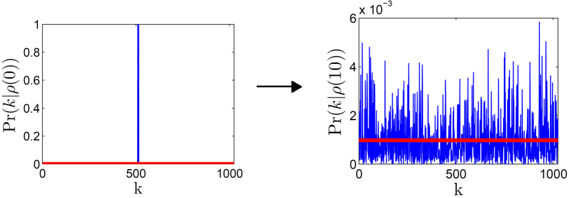
The system must be allowed to evolve for a sufficient amount of time for the state to spread out from a distribution with support on initial eigenstate of to one that obeys for our result to hold (see Fig. 1). We refer to the earliest such time as the equilibration time, which we denote . For an individual system, we also require that for most that is nearly maximally spread out. If the Hamiltonian is drawn from an ensemble, it is then possible to define an equilibration time such that almost all Hamiltonians drawn from the ensemble achieve ITE with respect to and :
Lemma 1.
Almost all Hamiltonians sampled from an ensemble of Hamiltonians equilibrate information theoretically with respect to a fixed observable and time , in the limit as , if the ensemble average and variance (denoted and respectively) of the outcome variance obey for all
| (3) | ||||
| (4) |
Proof is given in the supplemental material.
We now give our first evidence for universality by proving that ITE is typical for the important Gaussian Unitary Ensemble (GUE), which defines an invariant measure on the set of Hamiltonians. The GUE is the appropriate model a highly successful model for many properties of complex physical systems with no hidden symmetries Mehta (2004).
Theorem 2.
Take a non-degenerate observable acting on , and an initial pure state which is an eigenstate of . Almost all Hamiltonians drawn from GUE then equilibrate information theoretically with respect to and in the limit as for .
The proof is in the supplemental material. This theorem tells us the remarkable result that, as increases, the overwhelming majority of Hamiltonians will cause an initially pure, localized state to spread out over the non-degenerate eigenbasis of in a sufficiently uniform manner, to become practically indistinguishable from the microcanonical state for any . Thanks to decades of numerical studies of GUE as a model of complex many-body systems Beenakker (1997) and few-body quantum chaos systems Haake (2004), it is known that GUE is a good predictor of short-range spectral fluctuations Bohigas et al. (1984), and low-order moments of eigenvector components Kus and Haake (1988); Kus and Zyzckowski (1991), but not a good predictor of long-range spectral fluctuations Haake (2004). Our proof of the smallness of the fluctuations using GUE (for ) depends only on low-order moments of the eigenvector components, i.e., unitary -design condition with =8 Dankert et al. (2009) (see supplementary material for details). Hence we expect this aspect of the GUE model to be reflected in physically relevant Hamiltonian systems. However, we do not expect the GUE prediction for the equilibration time-scale to be physically relevant (clearly the value of for GUE is unrealistically short) because it depends on long-range spectral fluctuations. We now confirm both of these expectations for two RMEs consisting of many-body spins with two-body interactions, and conclude by demonstrating ITE with respect to tensor product measurements on a physically relevant time-scale in some example model systems.
We construct an ensemble of random local Hamiltonians (RLH) on spins, consisting of –body interactions between –level quantum systems, as follows:
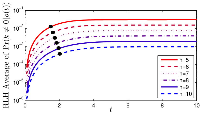
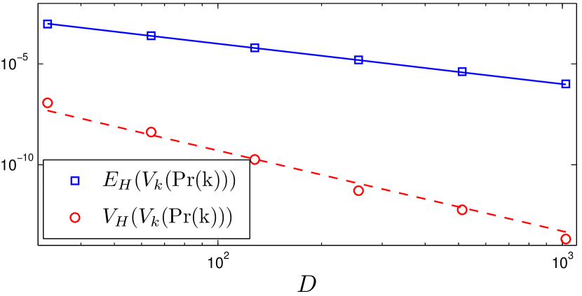
where , and each and is a Gaussian random variable with mean and variance . We consider the observable , corresponding to a non-degenerate projective measurement in the eigenbasis of . RLH is clearly invariant under permutation of qubit labels and local rotations of each qubit, and therefore our results also apply to any that differs from by local rotations. Fig. 2 shows that pure states evolving under individual elements of RLH approach equilibrium as increases. We estimate the equilibration time using the location of the inflection points of the curves in Fig. 2, and find it scales as , which is characteristic of quantum chaotic systems Emerson and Ballentine (2001a, b); Haake (2004). Fig. 3 shows that the outcome variance for a typical Hamiltonian chosen uniformly from the RLH ensemble satisfies the requirementes of Lemma 1, which implies that almost all RLH Hamiltonians will equilibrate information theoretically with respect to any non-degenerate measurement in the class as for any . We further strengthen the physical relevance of this result by showing that ITE still holds for when the 2-local Hamiltonians are constrained to have nearest-neighbor interactions in one– and two–dimensions (see supplemental material).
We now give two simple examples of individual model systems that exhibit information theoretic equilibration: a many-body system that is a two-field variant of the Heisenberg Hamiltonian and a one-body chaotic model, the quantum kicked top. The two-field variant of the Heisenberg mode consists of -spins arranged in a line with periodic boundary conditions:
| (5) |
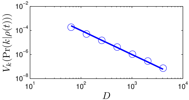
We choose this Hamiltonian because it is highly structured local Hamiltonian that is not typical of RLH and yet it is unstructured enough to be non-integrable so there are no constants of motion that prevent equilibration on the full Hilbert space (otherwise ITE would be limited to the invariant subspaces fixed by the constants of motion). Figure 4 shows that the outcome variance of the probability distribution indeed scales as with respect to , corresponding to read-out of all spins in the computational basis. Hence Theorem 1 implies that information theoretic equilibration occurs for this simple many-body Hamiltonian with respect to a natural observable. This is evidence that our equilibration mechanism is not just a mathematical feature of random Hamiltonian ensembles but occurs also in a simple, physically accessible many-body model. We also demonstrate ITE for the quantum kicked top in a regime of global chaos with respect to non-degenerate measurements in the basis (see supplemental material) and physically accessible times.
Conclusion. We have demonstrated a novel mechanism for equilibration that holds very broadly for the probability distributions of even maximally fine-grained measurements on pure quantum states of closed Hamiltonian systems. Remarkably, this information theoretic equilibration is observed to hold without requiring any form of decoherence or restricting to local or otherwise coarse-grained measurements. This is because, in the typical case of a complex system, the dynamical pure-state quantum fluctuations, though finite, do not lead to a breakdown of correspondence with the equilibrium state (contrary to a common implicit assumption, see Refs. Habib S. and H. (1998); Zurek (1998); Popescu et al. (2006)) because they become unobservably small under purely statistical considerations (in the limit of large ) after the equilibration time-scale. Our key insight is that although dynamical pure states of complex systems exhibit coherent fluctuations away from true micro-canonical equilibrium, their detection in practice requires extraordinary experimental resources, such as collecting measurement outcomes from repetitions of the experiment, or pre–computation of the location of the dynamical state in a -dimensional Hilbert space, or performing joint (entangling) measurements on identical copies of the system. In the absence of such resources, by Theorem 1 we see that after some finite time, the empirical probability distributions for dynamical pure states of complex quantum systems cannot be distinguished from the micro–canonical equilibrium state.
Appendix A Proof of Theorem 1
-
Proof of Theorem 1.
The first step of the proof is to demonstrate that if w1e take samples from the uniform distribution then the probability of obtaining distinct outcomes is nearly . Since there are ways unique items can be selected from a set of and since there are possible selections of items, we have that the probability of seeing no coincidences if the actual distribution is the uniform distribution is
(6) This implies that coincidental outcomes are unlikely unless .
Now let us assume that the true probability distribution is not uniform, but rather a distribution with outcome variance . We compare this to a distribution with that has the highest probability of coincidence for some outputs. Using the the definition of variance, , expanding the sum and using , we find
(7) The probability that no coincidental measurements are observed after measurements is therefore at least
(8)
Let the event denote the observation that unique measurement outcomes are observed, be the event where at least one measurement outcome is repeated, be the model that prescribes a uniform probability distribution to the outcomes, be the model that the probability distribution has outcome variance , and be the sequence of samples yielded by the device.
Since the underlying distribution is drawn from a distribution over distributions on that is invariant under permutations of , , where is a permutation of . We therefore see that all sequences of measurement outcomes that are equivalent up to permutations of labels provide equivalent evidence for model . Since is the uniform distribution, for any permutation . It is then clear that the labels of the outcomes observed cannot be used to distinguish between model and . We therefore can, without loss of generality, choose the label of the outcomes such that the first outcome observed is outcome , the second unique outcome observed is an so forth. From this perspective, it is clear that the differences between both models only become apparent in the distribution of coincidental outcomes. Our proof then follows from Bayes’ theorem and by showing that the probability of a coincidental outcome is small unless .
Note that the preceding argument effectively prevents coarse graining from allowing us to distinguish the two distributions with high probability using a small number of measurements because the probability of correctly guessing a coarse graining that assigns high probability to particular coarse–grained outcomes is (given the assumption of permutation invariance).
There are two possible scenarios: either does not contain any repeated sample labels or contains at least one repeated sample label. We will first assume that the entries of are unique, which we denote event . Bayes’ Theorem then implies
| (9) |
From our previous discussion, we see that
| (10) |
These results, and the fact that give us
| (11) |
We apply Taylor’s Theorem to the denominator of (11) and find that
| (12) |
and similarly
| (13) |
This shows us that the support provided by event for either hypothesis is small unless .
Our next step is to formally show that a typical data set will be, with high probability, uninformative unless . This follows from a concentration of measure argument over for the posterior probability distribution. The average over of the posterior probability is
| (14) |
Using , and we find from (12) that (14) implies
| (15) |
A similar calculation gives the variance as
| (16) |
Therefore, Chebyshev’s inequality implies that the probability of a given data set deviating substantially from the expectation value is
| (17) |
Using this result in concert with (15) implies that, with high probability, the posterior probability distribution after taking samples will obey
| (18) |
The result of Theorem 1 then follows from choosing the prior .
∎
Appendix B Proof of Lemma 1
-
Proof of Lemma 1.
Eqns. (3), (4) and Chebyshev’s inequality imply that in the limit of large , the outcome variance of for is concentrated around . In particular, for any we have from Chebyshev’s inequality and (4) that
(19) where is the appropriate measure for the ensemble . In other words, the outcome variance for an individual system are very close to the ensemble average.
We can see that almost all Hamiltonians will have outcome variance in the limit of large via the following argument. To compute the probability that the outcome variance of a particular Hamiltonian scaling as for some , we set . Equation (19) then implies that the probability of such an event scales at most as , which vanishes in the limit of large unless . Almost all Hamiltonians chosen from the ensemble therefore have outcome variance in the limit of large if .
Next we will show that this implies information theoretic equilibration with respect to the observable and time . We know that almost all Hamiltonians drawn from the ensemble will satisfy the requirements of Theorem 1. Let us then consider a decision problem where we are maximally ignorant whether the state is a distribution that is uniform or one with outcome variance . This corresponds to taking an equal a priori probability of for both outcomes. The theorem then implies that the probability of distinguishing the measurement statistics from those that would be expected from the uniform distribution is at most . Therefore, samples are needed to distinguish the two possible models with probability greater than for any fixed . We then see from Definition 1 that almost all Hamiltonians drawn from this ensemble will equilibrate information theoretically with respect to and for any as . ∎
Appendix C Unitary t-design Condition for Information Theoretic Equilibration
We now discuss how the unitary, , which transforms the eigenbasis of to that of the observable can be used to understand the equilibration properties of . Working in the eigenbasis of , we can write , where , and are the energy eigenvalues of . Given an initial pure state , the measurement outcome probabilities can be written as
| (20) |
Information theoretic equilibration follows from , which in turn requires that we know certain properties of . It is not difficult to see that and can be concisely represented by
| (21) | ||||
| (22) |
where , , and
| (23) | ||||
| (24) |
We refer to a term of the form in the sum in (21) as a –term because there are two basis change matrices acting on each factor space. The analogous terms in (22) will be called –terms; furthermore, can be expressed as a polynomial (meaning that all terms in the expansion of the outcome variance are at most terms). It can be easily checked using (2) and Chebyshev’s inequality that 3 and (4) hold if the – and –terms scale as and respectively. This shows that we can reduce the question of whether typical Hamiltonians drawn from an ensemble equilibrates information theoretically with respect to an observable and time to a question about the properties of these terms.
The scalings given in eqns. 3 and (4) are satisfied if the matrix elements of , namely the Hamiltonian eigenvector components, satisfy a unitary -design condition Dankert et al. (2009), which means that these matrix elements reproduce Haar-randomness for polynomials of degree at most . A similar connection was identified recently for subsystem equilibration in Refs. Brandao et al. (2011); Masanes et al. (2011); Znidaric et al. (2011), which required a unitary -design. For microcanonical equilibration, we must also ensure that is sufficiently small to imply a concentration of measure for via Chebyshev’s inequality. The resulting expression is an –polynomial and hence a unitary -design condition is sufficient to imply that information theoretic equilibration with respect to local qubit measurements and is typical for individual systems from the ensemble (using Theorem 1 and Lemma 1).
Appendix D Equilibration for Nearest Neighbor Hamiltonians
Previously, we showed numerically that random local Hamiltonians on a complete graph equilibrate information theoretically with respect to observables that are local rotations of for non–degenerate and an eigenstate of . Although some physical systems, such as the Bardeen–Cooper–Schrieffer Hamiltonian for low–temperature superconductivity Wu et al. (2002), can be represented as random local Hamiltonians on a complete graph, many physically relevant Hamiltonians have interactions that are constrained to nearest neighbors. We consider two relevant cases. First, we consider random local Hamiltonians with nearest neighbor interactions on lines with periodic boundary conditions. We then consider random local Hamiltonians on square lattices with periodic boundary conditions. In both cases, we see compelling numerical evidence for information theoretic equilibration with respect to for non–degenerate .
Random local Hamiltonians on a line– We will now consider Hamiltonians of the form
| (25) |
where the sum over refers to a sum over nearest neighbor and and . In this case, such that only interactions between qubits and are permitted if or . Similarly to the RLH ensemble, we take and to be Gaussian random variables with mean and variance .
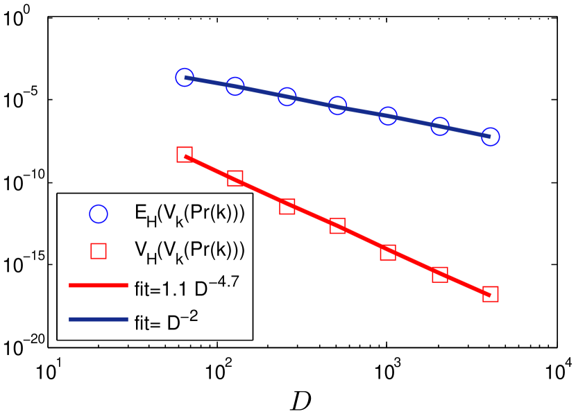
Figure 5 shows that typical members drawn from this constrained ensemble of random local Hamiltonians also achieve information theoretical equilibrium with respect to . We see from the results that the ensemble expectation of the outcome variance scales as and that the ensemble variance of the outcome variance scales as . We know from the results of Lemma 1 require that if the ensemble average and variance of at most as and respectively in order to guarantee that a Hamiltonian sampled uniformly from the ensemble will, with high probability, equilibrate information theoretically with respect to the observable. We therefore conclude from this data that information theoretic equilibration with respect to non–degenerate measurements in the eigenbasis of is generic for members of this ensemble of random local Hamiltonians.
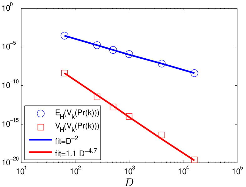
Random local Hamiltonians on a square lattice– Next we examine the issue of whether typical members of the ensemble of random local Hamiltonians that are constrained to have only nearest neighbor interactions between qubits on a square lattice equilibrate information theoretically with respect to computational basis measurements. The ensemble of Hamiltonians is similar to that in (25) except now we permit two qubits to interact if the two qubits are adjacent vertices on a square lattice. Note that we do not require that the overall shape of the lattice is a square. Specifically, we consider lattices with a number of qubits . In the case of the lattice is uniquely a square of qubits. In the case of , there is an ambiguity in that the lattice can be expressed as an array of qubits or qubits. We examine the former configuration because it is less like the D case.
Figure 6 shows that Hamiltonians drawn uniformly from this ensemble of Hamiltonians constrained to nearest neighbor interactions on a square lattice, with high probability, equilibrate information theoretically with respect to computational basis measurements for exactly the same reasons as the one–dimensional case discussed above. We also should note that although we have only studied equilibration with respect to a computational basis measurement, the results trivially also hold for local rotations of the computational basis because both the one– and two–dimensional ensembles are invariant with respect to single qubit rotations of any and all qubits.
Appendix E Equilibration Time for a variant of the Heisenberg Model
In the main body of the text, it was claimed that a variant Heisenberg model:
| (26) |
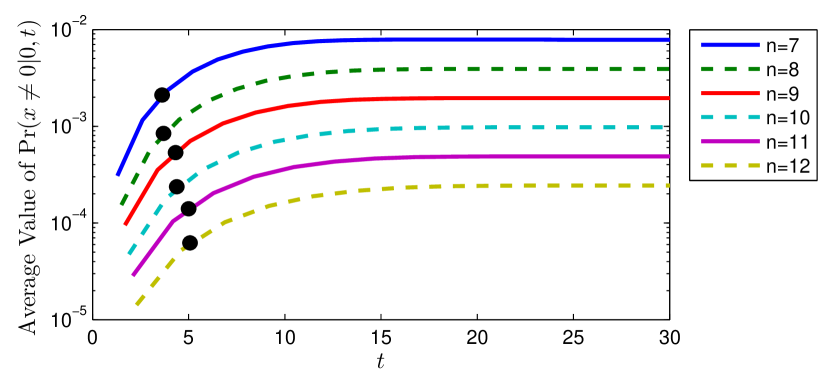
has an equilibration time of . This fact can be seen in Figure 7 where we plot the average probability, over , of an initial eigenstate of being measured in the state after evolution under the Hamiltonian for time . We see from the figure strong evidence for equilibration of the measurement outcome.
The equilibration times do not scale as smoothly with as the data considered for the RLH ensemble. The reason for this discrepancy is that the ratio of spins experiencing a magnetic field in the direction to those experiencing a field in the direction varies with . If is even, then the ratio will be ; however, if is odd then there will be an excess of spins experiencing a transverse field in the direction. This difference causes the equilibration times to vary with the parity of . We do see evidence though in Figure 7 that ; although given the small range for the fit, the precise functional dependence of on is not certain.
Appendix F Equilibration for a One–Body Quantum Chaotic System
Finally we show that information theoretic equilibration of pure states occurs also for an individual system consisting of a one-body dynamical model associated with global classical chaos. In particular we consider a variant of the quantum kicked top, described by the Floquet map Haake (2004):
| (27) |
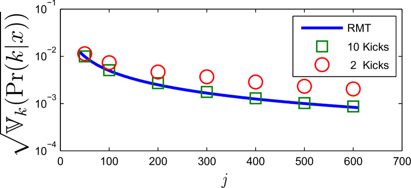
where is a vector of angular momentum operators, is the moment of inertia tensor, which is diagonal with entries , is a vector of kick–strengths and . The dimension of the system is where is the total angular momentum quantum number. Fig. 8 shows that for a set of chaotic parameters for and , roughly kicks (applications of ) are needed in order for , and hence for Theorem 1 to apply.
Appendix G Inferring Equilibration of RLH from Terms
We showed previously that if the Hamiltonian is sufficiently complex, meaning that the change of basis matrix satisfies a condition similar to an –design condition, then equilibration theoretic equilibration is generic for Hamiltonians drawn uniformly from the ensemble. Here we use this insight to infer from the properties of the terms of RLH Hamiltonians that information theoretic equilibration is generic.
In order to show this, we need to estimate the ensemble means and variances of the dominant terms (in the limit of large ). If the initial state preparation is and measurement outcome is considered then the relevant sum in computing the value of (which is needed in the computation of ) is
| (28) |
Here each summand is known as a term. It is easy to then see that in the limit of large and under the assumption of non–degenerate Hamiltonians, that terms with and will dominate other terms due to the fact that no phase cancellation appears in the sum over such terms. This means that the value of the outcome variance is dictated by the characteristic magnitude of such terms. In this case, we do not need to compute the –terms because trivially holds for RLH Hamiltonians.
Fig. 9 shows that the RLH average of the –terms agrees with the GUE predictions of scaling. We also find that the variance of the terms is which suggests that concentration of measure holds for the ensemble. This shows that the equilibriation properties observed for the RLH ensemble can also be inferred from the properties of the change of basis matrix .
Appendix H Proof of Theorem 2
We prove Theorem 2 in two steps:
- 1.
-
2.
We find the expectations of these expressions over the GUE eigenvalue distribution, and show that there exists a time such that for all , eqns. (3) and (4) hold. See Section H.2 for these expectations.
Since the calculations in this subsection require in depth knowledge of the properties of the Gaussian Unitary Ensemble (GUE), we will begin by giving a brief review of its properties Haake (2004); Mehta (2004); Balian (1968). GUE is the unique unitarily invariant distribution over Hermitian matrices that factorizes into a product of distributions each over an individual element of . In particular, each indepedent element of is an i.i.d. Gaussian random variable. A Hermitian matrix generated according to the GUE has diagonal elements that are real valued random variables each with distribution , and off-diagonal elements with real and imaginary parts that are random variables each with distribution . The variance is a free parameter, which is closely related to the expected maximum energy eigenvalue as well as the ensemble average energy level spacing.
While many aspects of GUE have been shown to accurately model complex quantum systems, there are known limitations to using GUE as a model of such systems which deserve mention before we proceed. First, the average level density, which takes the form of a semi-circle, and long-range spectral fluctuations for GUE are not good models for the corresponding properties of physically relevant Hamiltonian systems, even chaotic ones. In particular, for most natural systems, such as those with only two particle interactions, the norm of the Hamiltonian scales polynomially with the number of particles Linden et al. (2009). However, the expected norm of a GUE Hamiltonian scales polynomially in the Hilbert space dimension Haake (2004). As we will see below, this has a large impact on what might be called the equilibration time for these dynamical systems, which should therefore be taken with a grain of salt. Because of this, and in order to simplify calculations, we will follow the standard practice Masanes et al. (2011); Mehta (2004) of taking the variance .
The joint distribution over all elements of factorizes into a product of a distribution over eigenvectors, and a distribution over the energy eigenvalues of (see Mehta (2004) Theorem 3.3.1, or Haake (2004) Chapter 4). Further, the joint probability distribution over eigenvectors of is the same as that over the change of basis matrix , namely the Haar measure on the unitary group Haake (2004); Mehta (2004). Letting be the unitary which takes the eigenbasis of to that of , and working in the eigenbasis of , we can write
| (29) |
where , and are the energy eigenvalues of . We can therefore take separate expectations over eigenvectors and eigenvalues, namely, over the matrices and . can be expressed as
| (30) |
In the following we will write the expectation over the Haar measure on the unitary group of change of basis matrices , as , and for the expectation over the GUE eigenvalue distribution.
H.1 Expectations over eigenvectors
Lemma 2.
Take a non-degenerate observable acting on , an initial pure state which is an eigenstate of , and a unitary where is drawn uniformly at random from GUE. Then the variance of the measurement outcome probabilities over the Haar measure on the unitary group of change of basis matrices is given by:
| (31) |
where we have defined (this is often called the spectral form factor Haake (2004); Mehta (2004)).
Proof.
First, note that the squares of the outcome probabilities can be written in the form:
| (32) |
where is the complex conjugate of and
| (33) |
The expectation of the expression over Haar measure can be written as the projector onto the subspace spanned by the vectors
| (34) |
where , and the index runs over the permutations of the elements , and is the unitary permutting the first four factor spaces according to . It was shown in Brandao et al. (2011) that this projector is given by
| (35) |
where the matrix has components , and is number of cycles in the cycle decomposition of the permutation . We then have
| (36) |
where the inner products are given by:
Further, for , , , , and for all other .
Lemma 3.
Take a non-degenerate observable acting on , an initial pure state which is an eigenstate of , and a unitary where is drawn uniformly at random from GUE. Then the expectation of the measurement outcome probabilities for distributed according to the Haar measure on the unitary group is given by:
| (39) |
Proof.
This expectation can be calculated in a similar but simpler fashion as the variance in the previous lemma, so we leave the proof as an exercise. ∎
Lemma 4.
Take a non-degenerate observable acting on , an initial pure state which is an eigenstate of , and a unitary where is drawn uniformly at random from the GUE. Then the fourth moment of the measurement outcome probabilities over the Haar measure on the unitary group of change of basis matrices is given by:
| (40) |
where is a matrix with components .
Proof.
The fourth power of the outcome probabilities can be written in the form:
| (41) |
where and are defined analogously to (33), but with twice the number of tensor factors. Further, the average of the expression over Haar measure can be written as the projector onto the subspace spanned by the vectors
| (42) |
where the index runs over the permutations of the elements , and is the unitary permuting the first eight factor spaces according to .
We will now determine the asymptotic scaling of the following expression with :
| (43) |
by finding an approximation for . Recall that the matrix has components , where is number of cycles in the cycle decomposition of the permutation . It is clear that the diagonal components of are all equal to , and all other components of are strictly , as the identity permutation is the only one with cycles. Letting we have
| (44) |
which converges to in the limit if and only if . Because is of fixed size and all its elements are , we have for sufficiently large. Therefore, , which implies that
| (45) |
Next, it is not difficult to see that all components of are equal to or . Therefore, we can split the sum in (43) as
| (46) |
where we have used that for all , and has all components . ∎
H.2 Expectations over GUE eigenvalues
Our next step towards proving Theorem 2 is to find the GUE average of the the spectral form factor , which appears in Lemmas 2 and 3. The joint distribution over the un-ordered energy eigenvalues of a GUE matrix is given by (see Mehta (2004) Theorem 3.3.1, or Haake (2004) Chapter 4):
| (47) |
where we define . Integration of over variables gives the m-point correlation function (Mehta (2004) 6.1.1)
| (48) |
where . By Mehta (2004) Theorem 5.1.4, this can be written as:
| (49) |
where , and the are the harmonic oscillator wave-functions , with the Hermite polynomials (see Mehta (2004) section 6.2).
H.2.1 Calculation of
Our next goal is to evaluate the expression . Expanding out the trace and grouping terms, we have
| (50) |
Using the invariance of the joint distribution under permutations of the energies, and the definition of the 2-point correlation function, this becomes
| (51) |
It is well known that for large the function follows the so called Wigner semi-circle law Mehta (2004) (with ):
| (52) |
where is the Heavyside step function. For large we then have:
| (53) |
where is the first Bessel function of the first kind. It should also be noted that, the limit of the function is generally taken by rescaling (often called ‘unfolding’ - see Guhr et al. (1998) section III.A.1) the energy level density as well as the energies by the local mean spacing Haake (2004); Mehta (2004). In taking this limit and the integrals for we have followed the the procedure of Mehta (2004) Appendices 10, and 11.
H.2.2 Equilibration time
Now that we have the GUE expectation of the spectral form factor, we can use Lemma 3, to find the full expectation over eigenvectors and eigenvalues of the outcome probabilities:
| (54) |
Notice that if , then
| (55) |
In particular, if is large, then the GUE expectation of the probability distribution from (55) is essentially the uniform distribution. We therefore take the equilibration time to be defined by the condition
| (56) |
It is clear that the second term in (H.2.1) satisfies:
| (57) |
This shows that there exists a finite time such that for all .
In order to get a sense of the equilibration time (keeping in mind our previous comments on GUE energy spectra), note that the condition on the equilibration time (56) is essentially that
| (58) |
Using the fact that for we can approximate , it the follows that the equilibration time is
| (59) |
H.2.3 GUE expectation of first and second power
Our next step towards a proof of Theorem 2 involves evaluating the expectation values over the spectrum that are needed to prove eqns. (3) and (4) for GUE Hamiltonians. First, from the previous section we have that there exists a finite time such that for all . Using Lemma 3, and the above spectral expectation, we have
| (60) |
which proves that for all , eqn. (3) holds for GUE Hamiltonians.
Next, Lemma 2 implies that
| (61) |
In the next section we will show that for , . Using this along with in the above, we find
| (62) |
which proves that for all , eqn. (3) holds.
H.2.4 Bounding
In order to simplify the derivation of our upper bounds, we define
We can expand the triple sum into three parts depending on whether are: (i) all distinct, (ii) only two equal, or (iii) all equal, which upon integration over the remaining energies, give terms of the form:
-
(i)
,
-
(ii)
,
-
(iii)
.
By expanding and , we find products of integrals of terms of the form , as well as , and
| (64) |
We will bound the magnitude of these terms in a similar fashion as was done in Masanes et al. (2011). Note that the integral of (64) is just
| (65) |
where is the projector onto the D-dimensional lower-energy subspace spanned by the harmonic oscillator wave-functions, and is the position operator. Using the Cauchy-Schwartz inequality twice on (65), we find:
| (66) |
A similar argument also shows that terms with integrands of the form are also bounded by . Using these bounds, we then have
| (67) |
Next recall that
| (68) |
which approaches as . The equilibration condition (56) requires that for , and if this is satisfied, then for all , we have .
H.2.5 GUE expectation of fourth power
The final quantity that we need to prove Theorem 2 is the asymptotic scaling of the GUE average of the fourth moment of where for an eigenvector of the observable. This quantity shows a concentration of measure for the outcome variance of , which will allow us to conclude that individual Hamiltonians drawn from the GUE will information theoretically equilibrate with high probability. Specifically, we show that for we have that . Recalling the form of from Lemma 4, we see that it is sufficient to show that for , we have , for all permutations .
Calculating some explicit examples of
we see that these are of the general form
| (70) |
where , and
| (71) |
and if then the corresponding does not appear in the product (and similarly for ). For example, there is a term arising from , and a term arising from . The expectations can then be bounded in a similar fashion to Appendix H.2.4. In particular, we can expand the sums in the product of the terms into various parts depending on which indices are equal or not equal, just as was done for expression (LABEL:splitting_sums). These will then give a constant factor, and various combinations of integrals of m-point correlation functions. Each of the integrals with 2-point or higher order correlation functions can be bounded by , just as was done for eqn. (64). We will then be left with various powers of integrals of the form which as we have seen approach as , and so are irrelevant for the regime. The only remaining question then is power of the constant factor for each term. It is not difficult to see that a power of arises from each pairing with . For example, the expectation of the term gives a contribution of (this is in fact the infinite time limit). From the constraint (71), it is not difficult to see that is the highest power of which can arise. This shows that for
| (72) |
Putting all of the above together, we have:
-
Proof of Theorem 2.
Expanding the outcome and ensemble variances and using (62) and (72), we find that, for ,
(73) Then using the Cauchy-Schwartz inequality for expectations and (60), we have:
(74) This proves that . Chebyshev’s inequality then implies (in the same fashion as (19)) that with high probability over . Theorem 1 then implies that samples are required to distinguish the from the uniform distribution for , which was shown in (59). Since a particular Hamiltonian is specified using , even drawing a random Hamiltonian from GUE requires arithmetic operations. Therefore it follows from Definition 1 and Lemma 1 that almost all GUE Hamiltonians equilibrate information theoretically for with high probability. ∎
Acknowledgements. We thank Fernando Brandão, Carl Caves, David Cory, Patrick Hayden, Daniel Gottesman, and Victor Veitch for insightful comments. We acknowledge funding from CIFAR, Ontario ERA, NSERC, US ARO/DTO and thank the Perimeter Institute for Theoretical Physics where this work was brought to completion.
References
- Popescu et al. (2006) S. Popescu, A. J. Short, and A. Winter, Entanglement and the Foundations of Statistical Mechanics, Nature Physics 2, 754 (2006), arXiv:0511225.
- Goldstein et al. (2010) S. Goldstein, J. L. Lebowitz, R. Tumulka, and N. Zanghì, Long-time behavior of macroscopic quantum systems: Commentary accompanying the english translation of John von Neumann’s 1929 article on the quantum ergodic theorem (2010), arXiv:1003.2129.
- Rigol et al. (2008) M. Rigol, V. Dunjko, and M. Olshanii, Thermalization and its mechanism for generic isolated quantum systems, Nature 452, 854 (2008).
- Venuti and Zanardi (2010) C. L. Venuti and P. Zanardi, Unitary equilibrations: Probability distribution of the Loschmidt echo, Phys. Rev. A 81, 022113 (2010).
- Linden et al. (2009) N. Linden, S. Popescu, A. J. Short, and A. Winter, Quantum mechanical evolution towards thermal equilibrium, Phys. Rev. E 79, 061103 (2009).
- Brandao et al. (2011) F. Brandao, P. Cwiklinski, M. Horodecki, P. Horodecki, J. Korbicz, and M. Mozrzymas, Convergence to equilibrium under a random hamiltonian (2011), arXiv:1108.2985.
- Masanes et al. (2011) L. Masanes, A. J. Roncaglia, and A. Acin, The complexity of energy eigenstates as a mechanism for equilibration (2011), arXiv:1108.0374.
- Lloyd (1988) S. Lloyd, Black holes, demons and the loss of coherence: How complex systems get information, and what they do with it, Ph.D. thesis, Rockefeller University, New York (1988).
- Goldstein et al. (2006) S. Goldstein, J. L. Lebowitz, R. Tumulka, and N. Zanghì, Canonical typicality, Phys. Rev. Lett. 96, 050403 (2006).
- Gemmer et al. (2004) J. Gemmer, M. Michel, and G. Mahler, Quantum Thermodynamics: Emergence of Thermodynamic Behavior within Composite Quantum Systems. (Springer: Berlin, 2004).
- Znidaric et al. (2011) M. Znidaric, C. Pineda, and I. García-Mata, Non-Markovian behavior of small and large complex quantum systems, Phys. Rev. Lett. 107, 080404 (2011), arXiv:1104.5263.
- Reimann (2010) P. Reimann, Canonical thermalization, New Journal of Physics 12, 055027 (2010).
- Short (2011) A. J. Short, Equilibration of quantum systems and subsystems, New Journal of Physics 13, 053009 (2011).
- Short and C. (2012) A. J. Short and F. T. C., Quantum equilibration in finite time, New Journal of Physics 14, 013063 (2012), arXiv:1110.5759.
- Reimann and Kastner (2012) P. Reimann and M. Kastner, Equilibration of isolated macroscopic quantum systems, New Journal of Physics 14, 043020 (2012).
- Peres (1984) A. Peres, Ergodicity and mixing in quantum theory. I, Phys. Rev. A 30, 504 (1984).
- Srednicki (1994a) M. Srednicki, Chaos and quantum thermalization, Phys. Rev. E 50, 888 (1994a).
- Srednicki (1994b) M. Srednicki, Does quantum chaos explain quantum statistical mechanics? (1994b), arXiv:9410046.
- Gaspard (2005) P. Gaspard, Chaos, Scattering and Statistical Mechanics, Cambridge Nonlinear Science Series (Cambridge University Press, 2005), ISBN 9780521018258.
- Dorfman (1999) J. R. Dorfman, An Introduction to Chaos in Nonequilibrium Statistical Mechanics (1999).
- Mehta (2004) M. L. Mehta, Random Matrices; 3rd ed. (Elsevier, San Diego, CA, 2004).
- Haake (2004) F. Haake, Quantum Signatures of Chaos Edition (Springer-Verlag New York, 2004).
- Cho et al. (2005) H. Cho, T. D. Ladd, J. Baugh, D. G. Cory, and C. Ramanathan, Multispin dynamics of the solid-state nmr free induction decay, Phys. Rev. B 72, 054427 (2005).
- Habib S. and H. (1998) S. K. Habib S. and Z. W. H., Decoherence, chaos and the correspondence principle, Phys. Rev. Lett. 80, 4361 (1998).
- Zurek (1998) W. Zurek, Decoherence, chaos, quantum-classical correspondence and the arrow of time, Acta Physica Polonica B29, 3689 (1998).
- Nielsen and Chuang (2000) M. A. Nielsen and I. Chuang, Quantum Computation and Quantum Information (Cambridge University Press, 2000).
- Emerson and Ballentine (2001a) J. Emerson and L. Ballentine, Characteristics of quantum-classical correspondence for two interacting spins, Phys. Rev. A 63, 052103 (2001a).
- Emerson and Ballentine (2001b) J. Emerson and L. E. Ballentine, Quantum-classical correspondence for the equilibrium distributions of two interacting spins, Phys. Rev. E 64, 026217 (2001b).
- Kus and Haake (1988) M. J. Kus, M. and F. Haake, Universality of eigenvector statistics of kicked tops of different symmetries, J. Phys. A: Math. Gen. 21, L1073 (1988).
- Kus and Zyzckowski (1991) M. Kus and K. Zyzckowski, Relative randomness of quantum observables, Phys. Rev. A 44, 956 (1991).
- Beenakker (1997) C. W. J. Beenakker, Random-matrix theory of quantum transport, Rev. Mod. Phys. 69, 731–808 (1997).
- Bohigas et al. (1984) O. Bohigas, M. J. Giannoni, and C. Schmit, Characterization of chaotic quantum spectra and universality of level fluctuation laws, Phys. Rev. Lett. 52, 1 (1984).
- Dankert et al. (2009) C. Dankert, R. Cleve, J. Emerson, and E. Livine, Exact and approximate unitary 2-designs and their application to fidelity estimation, Phys. Rev. A 80, 012304 (2009), arXiv:0606161.
- Wu et al. (2002) L.-A. Wu, M. S. Byrd, and D. A. Lidar, Polynomial-time simulation of pairing models on a quantum computer, Phys. Rev. Lett. 89, 057904 (2002).
- Balian (1968) R. Balian, Random matrices and information theory, Il Nuovo Cimento B (1965-1970) 57, 183 (1968).
- Guhr et al. (1998) T. Guhr, A. Müller-Groeling, and H. A. Weidenmüller, Random-matrix theories in quantum physics: common concepts, Physics Reports 299, 189 (1998).