Will-be-set-by-IN-TECHExtending cosmology: the metric approach Mexico

1 Introduction

In this chapter it is shown how the introduction of a fundamental constant of nature with dimensions of acceleration into the theory of gravity makes it possible to extend gravity in a very consistent manner. In the non-relativistic regime a MOND-like theory with a modification in the force sector is obtained. This description turns out to be the the weak-field limit of a more general metric relativistic theory of gravity. The mass and length scales involved in the dynamics of the whole universe require small accelerations which are of the order of Milgrom’s acceleration constant, it turns out that this relativistic theory of gravity can be used to explain the expansion of the universe. In this work it is explained how to build that relativistic theory of gravity in such a way that the overall large-scale dynamics of the universe can be treated in a pure metric approach without the need to introduce dark matter and/or dark energy components.

Cosmological and astrophysical observations are generally explained introducing two unknown mysterious dark components, namely dark matter and dark energy. These ad hoc hypothesis represent a big cosmological paradigm, since they arise due to the fact that Einstein’s field equations are forced to remain unchanged under certain observed astrophysical phenomenology.

A natural alternative scenario would be to see whether viable cosmological solutions can be found if dark unknown entities are assumed non-existent. The price to pay with this assumption is that the field equations of the theory of gravity need to be extended and so, new Friedmann-like equations will arise. The most natural approach to extend gravity arises when a metric extension $f(R)$ is introduced into the theory (see e.g. Capozziello and Faraoni, 2010, and references therein).

In a series of recent articles, Carranza et al. (2012); Mendoza et al. (2011); Bernal, Capozziello, Hidalgo and Mendoza (2011); Hernandez et al. (2010, 2012b); Bernal, Capozziello, Cristofano and de Laurentis (2011); Mendoza et al. (2012) have shown how relevant the introduction of a new fundamental physical constant $\mathsf{a}_{0}\approx 10^{-10}\textrm{m}/\textrm{s}^{2}$ with dimensions of acceleration is in excellent agreement with different phenomenology at many astrophysical mass and length sizes, from solar-system to extragalactic and cosmological scales. The introduction of the so called Milgrom’s acceleration constant $\mathsf{a}_{0}$ in a description of gravity means that any gravitational field produced by a certain distribution of mass (and hence energy) needs to incorporate the acceleration $\mathsf{a}_{0}$ together with Newton’s gravitational constant $G$ and the speed of light $c$ in the description of gravity.

In section 2 it is shown, through a description of an extended Newtonian gravity scenario, the advantages of working with a modification of gravity dependent on the mass and lengths associated with the dimensions and masses of the sources that generate the gravitational field, and not with the dynamical acceleration they produce on test particles. Section 3 describes how it is possible to build a metric theory of gravity which generalises the extended Newtonian description mentioned in section 2 and section 4 interconnects this extended relativistic description of gravity with a metric description of gravity for which the energy-momentum tensor appears in the gravitational field’s action. On section 5 we use the developed theory of gravity for cosmological applications in a dust universe and see how it is a coherent representation of gravity at cosmological scales. Finally on section 6, we discuss the consequences of the developed approach of gravity and some of the future developments of the theory.

2 Extended Newtonian gravity

Milgrom (1983, 2008, 2010) constructed a MOdified Newtonian Dynamics (MOND) theory, based on the introduction of a fundamental constant of nature $\mathsf{a}_{0}=1.2\times 10^{-10}\textrm{m}\,\textrm{s}^{-2}$ in such a way that the acceleration experienced by a test particle on a gravitational field produced by a point mass source $M$ is such that:

$$a=\left\{\begin{array}[]{c l}&-\frac{GM}{r^{2}},\qquad\qquad\text{for}\qquad\qquad a\gg\mathsf{a}_{0},\\ &-\frac{\sqrt{\mathsf{a}_{0}GM}}{r},\qquad\text{\ \ for}\qquad\qquad a\ll\mathsf{a}_{0},\end{array}\right.$$ (1)

where $r$ is the radial distance to the central mass. In other words, for accelerations $a\gg\mathsf{a}_{0}$, Newtonian gravity is recovered and new MONDian effects are expected to appear for accelerations $a\lesssim\mathsf{a}_{0}$. The strong $a\ll\mathsf{a}_{0}$ MONDian regime means that Kepler’s third law is not valid since for a circular orbit about the central mass $M$, the acceleration $a=v/r$, where $v$ is velocity of the test mass, and so $v=\left(\mathsf{a}_{0}GM\right)^{1/4}\propto M^{1/4}$, which is the Tully-Fisher relation (see e.g. Puech et al., 2010) for the case of a spiral galaxy and is the same relation experienced by wide-open binaries (Hernandez et al., 2012b) and by the tail of the “rotation curve” in globular clusters (Hernandez and Jiménez, 2012; Hernandez et al., 2012a).

In order to interpolate from the strong $a\gg\mathsf{a}_{0}$ Newtonian regime to the weak $a\ll\mathsf{a}_{0}$ one, the traditional MONDian approach is to construct a somewhat built-by-hand interpolation function $\mu(y)$ in such a way that

$$a\mu(y)=-\frac{GM}{r^{2}},$$ (2)

where

$$\mu(y)=\begin{cases}1,\qquad\text{for}\qquad y\gg 1,\\ y,\qquad\text{for}\qquad y\ll 1,\end{cases}\text{and}\quad y:=\frac{a}{\mathsf{a}_{0}}.$$

The usual approach to MOND as expressed by equation (2) means that Newton’s 2nd law of mechanics needs to be modified (see e.g. Bekenstein, 2006a). As explained by Mendoza et al. (2011), a better physical approach can be constructed if the modification is made in the force (gravitational) sector. Indeed, by the use of Buckingham’s theorem of dimensional analysis (cf. Sedov, 1959), the gravitational acceleration experienced by a test particle is given by

$$a=\mathsf{a}_{0}g(x),$$ (3)

where the dimensionless quantity

$$x:=\frac{l_{M}}{r},$$ (4)

and a mass-length scale

$$l_{M}:=\left(\frac{GM}{\mathsf{a}_{0}}\right)^{1/2}.$$ (5)

The length $l_{M}$ plays an important role in the description of the theory and is such that when $l_{M}\gg r$, the strong Newtonian regime of gravity is recovered and when $l_{M}\ll r$ the weak MONDian regime of gravity appears. As such, the dimensionless acceleration (or transition function) $g(x)$ is such that:

$$\frac{a}{\mathsf{a}_{0}}=g(x):=\begin{cases}x^{2},\qquad\text{when}\quad x\gg 1,\\ x,\qquad\text{ when}\quad x\ll 1.\end{cases}$$ (6)

In general terms, a mass distribution whose length is much greater than its associated mass-length $l_{\text{M}}$ is in the MONDian regime (since $x\ll 1$) and a mass distribution whose length is much smaller than its mass-length scale is in the Newtonian regime (since $x\gg 1$). The case $x=1$ can roughly be thought of as the point where the transition from the Newtonian to the MONDian regime occurs.

A general transition function $g(x)$ was built by Mendoza et al. (2011) taking Taylor expansion series about the correct MONDian and Newtonian limits, yielding:

$$g(x)=x\,\frac{1\pm x^{n+1}}{1\pm x^{n}}.$$ (7)

This non-singular function converges to the correct expected limits of equation (6) for any value of the parameter $n\geq 0$. As shown in Figure 1, the transition function $g(x)$ rapidly converges to the limit “step function”

$$g(x)\bigg{|}_{n\rightarrow\infty}=\begin{cases}x,\qquad\text{ for }0\leq x\leq 1,\\ x^{2},\qquad\text{for }x\geq 1,\end{cases}$$ (8)

when $n\gtrsim 3$. The parameter $n$ needs to be found empirically by astronomical observations. The value found by Mendoza et al. (2011) for the rotation curve of our galaxy is $n\gtrsim 3$ and the one found by Hernandez and Jiménez (2012); Hernandez et al. (2012b, a) is $n\gtrsim 8$, with a minus sign selection on the numerator and denominator on the right hand side of equation (7). These authors have shown that a large value of $n$ is coherent with solar system motion of planets, rotation curves of spiral galaxies, equilibrium relations of dwarf spheroidal galaxies and their correspondent relations in globular clusters, the Faber-Jackson relation and the fundamental plane of elliptical galaxies as well as with the orbits of wide binary stars. The $n=3$ model in which a small, but measurable transition is obtained, has also been tested on earth and moon-like experiments by Meyer et al. (2011) and Exirifard (2011) respectively, showing that it is coherent with such precise measurements. In fact, these experiments also validate all $n\geq 3$ models.

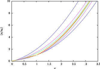
Figure 1: The figure taken from Mendoza et al. (2011) shows the acceleration function $a$ in units of Milgrom’s acceleration constant $\mathsf{a}_{0}$ as a function of the parameter $x$. The thick dash-dot curve is the extreme limiting value $n\to\infty$, i.e. $a/\mathsf{a}_{0}=x$ for $x\leq 1$ and $a/\mathsf{a}_{0}=x^{2}$ for $x\geq 1$. The curves above and below this extreme acceleration line represent values of $n=4,\ 3,\ 2,\ 1,$ for the minus and plus signs of equation (7) respectively. The extreme limiting curve has a kink at $x=1$.

Care must be taken when the introduction of a new fundamental constant of nature with dimensions of acceleration $\mathsf{a}_{0}$ is made. In fact, the introduction of $\mathsf{a}_{0}$ does not impose any kind causality arguments such as the ones given by the velocity of light $c$. In fact, one may think of $\mathsf{a}_{0}$ as a fundamental constant needed to transit from one gravity regime to another. In this respect for example, instead of using $\mathsf{a}_{0}$ as a fundamental constant, one may define

$$\Sigma_{0}:=\mathsf{a}_{0}/G=1.8\,\mathrm{kg}\,\mathrm{m}^{-2},$$ (9)

as the new fundamental constant of nature. The constant $\Sigma_{0}$, with dimensions of surface mass density, enters in the description of the gravitational theory in such a way that equations (3) and (5) are given by:

$$a=-G\Sigma_{0}g\left(l_{M}/r\right),\qquad l_{M}:=\left(M/\Sigma_{0}\right).$$ (10)

and the acceleration in the full MONDian regime and the corresponding Tully-Fisher relation are

$$a=-G\frac{\left(\Sigma_{0}M\right)^{1/2}}{r},\qquad v=G^{1/2}\Sigma_{0}^{1/4}M^{1/4}.$$ (11)

Also, a more manageable extended fundamental quantity, directly measurable through the Tully-Fisher relation, can be defined:

$$\epsilon_{M}:=\mathsf{a}_{0}G=8.004\times 10^{-21}\mathrm{m}^{4}\,\mathrm{s}^{-4}\,\mathrm{kg}^{-1},$$ (12)

with dimensions of velocity to the fourth over mass, for which

$$a=-\frac{\epsilon_{M}}{G}g\left(l_{M}/r\right),\qquad l_{M}:=\left(G^{2}\,M/\epsilon_{0}\right).$$ (13)

With this, the acceleration of a test particle in the full MOND regime and the Tully-Fisher relation are:

$$a=-\frac{\left(\epsilon_{M}\,M\right)^{1/2}}{r},\qquad v=\left(\epsilon_{M}\,M\right)^{1/4}.$$ (14)

The choice of a new fundamental constant of nature has many ways in which it can be introduced into the theory (Sedov, 1959). In this work, the use of $\mathsf{a}_{0}$ is kept as it is traditionally done, but we note the fact that $\epsilon_{0}$ is the best fundamental constant to use since it is directly measured through the flattened rotation curves of spiral galaxies.

The extended Newtonian model of gravity presented in this section is equivalent with MOND on spherical and cylindrical symmetry but deviates considerable from it for systems away from this symmetry (Mendoza et al., 2011). As we have already shown, there are however many advantages of using this approach, the most objective meaning that the modification is made on the force sector and not a modification on the dynamics.

3 Relativistic metric extension

Finding a relativistic theory of gravity for which one of its non-relativistic limits converges to MOND yields usually strange assumptions and/or complicated ideas (see e.g. Mishra and Singh, 2012; Blanchet and Marsat, 2012; Bekenstein, 2004). A good first approach was provided by a slight modification of Einstein’s field equations by Sobouti (2007), but the attempt is not complete.

In order to find an elegant and simple theory of gravity for which a MONDian solution is found, Bernal, Capozziello, Hidalgo and Mendoza (2011) used a metric correct dimensional interpretation of Hilbert’s gravitational action $S_{\text{f}}$ in such a way that:

$$S_{\text{f}}=-\frac{c^{3}}{16\pi GL_{M}^{2}}\int{f(\chi)\sqrt{-g}\,\mathrm{d}^{4}x},$$ (15)

which slightly differs from its traditional form (see e.g. Capozziello and Faraoni (2010); Sotiriou and Faraoni (2010); Capozziello et al. (2010)) since the following dimensionless quantity has been introduced:

$$\chi:=L_{M}^{2}R,$$ (16)

where $R$ is Ricci’s scalar and $L_{M}$ defines a length fixed by the parameters of the theory. The explicit form of the length $L$ has to be obtained once a certain known limit of the theory is taken, usually a non-relativistic limit. Note that the definition of $\chi$ gives a correct dimensional character to the action (15), something that is not completely clear in all previous works dealing with a metric description of the gravitational field. For $f(\chi)=\chi$ the standard Einstein-Hilbert action of general relativity is obtained.

On the other hand, the matter action has its usual form,

$$S_{\text{m}}=-\frac{1}{2c}\int{{\cal L}_{\text{m}}\,\sqrt{-g}\,\mathrm{d}^{4}x},$$ (17)

with ${\cal L}_{\text{m}}$ the matter Lagrangian density of the system. The null variations of the complete action, i.e. $\delta\left(S_{\text{H}}+S_{\text{m}}\right)=0$, yield the following field equations:

$$\begin{split}f^{\prime}(\chi)\,\chi_{\mu\nu}-\frac{1}{2}f(\chi)g_{\mu\nu}-L_{M}^{2}&\left(\nabla_{\mu}\nabla_{\nu}-g_{\mu\nu}\Delta\right)f^{\prime}(\chi)\\ &=\frac{8\pi GL_{M}^{2}}{c^{4}}T_{\mu\nu},\end{split}$$ (18)

where the dimensionless Ricci tensor $\chi_{\mu\nu}$ is given by:

$$\chi_{\mu\nu}:=L_{M}^{2}R_{\mu\nu},$$ (19)

and $R_{\mu\nu}$ is the standard Ricci tensor. The Laplace-Beltrami operator has been written as $\Delta:=\nabla^{\alpha}\nabla_{\alpha}$ and the prime denotes derivative with respect to its argument. The energy-momentum tensor $T_{\mu\nu}$ is defined through the following standard relation: $\delta S_{\text{m}}=-\left(1/2c\right)T_{\alpha\beta}\,\delta g^{\alpha\beta}$. In here and in what follows, we choose a ($+,-,-,-$) signature for the metric $g_{\mu\nu}$ and use Einstein’s summation convention over repeated indices.

The trace of equation (18) is:

$$f^{\prime}(\chi)\,\chi-2f(\chi)+3L_{M}^{2}\,\Delta f^{\prime}(\chi)=\frac{8\pi GL_{M}^{2}}{c^{4}}T,$$ (20)

where $T:=T^{\alpha}_{\alpha}$.

In order to search for a MONDian solution, Bernal, Capozziello, Hidalgo and Mendoza (2011) analysed the problem in two ways. First by performing an order of magnitude approach to the problem, and second, by doing a full perturbation analysis. Since the second technique is merely to fix constants of proportionality of the problem, their order of magnitude approach and its consequences are discussed in the remain of this section. Also, since we are interested at the moment on a point mass distribution generating a stationary spherically symmetric space-time, the trace equation (20) contains all the relevant information relating the field equations. At this point it is also useful to assume a power law form for the function

$$f(\chi)=\chi^{b}.$$ (21)

An order of magnitude approach to the problem means that $\mathrm{d}/\mathrm{d}\chi\approx 1/\chi$, $\Delta\approx-1/r^{2}$ and the mass density $\rho\approx M/r^{3}$. With this, the trace (20) takes the following form:

$$\chi^{b}\left(b-2\right)-3bL_{M}^{2}\frac{\chi^{(b-1)}}{r^{2}}\approx\frac{8\pi GML_{M}^{2}}{c^{2}r^{3}}.$$ (22)

Note that the second term on the left-hand side of equation (22) is much greater than the first term when the following condition is satisfied:

$$Rr^{2}\lesssim\frac{3b}{2-b}.$$ (23)

At the same order of approximation, Ricci’s scalar $R\approx\kappa=R_{\text{c}}^{-2}$, where $\kappa$ is the Gaussian curvature of space and $R_{\text{c}}$ its radius of curvature and so, relation (23) essentially means that

$$R_{c}\gg r.$$ (24)

In other words, the second term on the left-hand side of equation (22) dominates the first one when the local radius of curvature of space is much grater than the characteristic length $r$. This should occur in the weak-field regime, where MONDian effects are expected. For a metric description of gravity, this limit must correspond to the relativistic regime of MOND.

Under assumption (24), equation (22) takes the following form:

$$R^{(b-1)}\approx-\frac{8\pi GM}{3bc^{2}rL_{M}^{2\left(b-1\right)}}.$$ (25)

We now recall the well known relation followed by the Ricci scalar at second order of approximation at the non-relativistic level Landau and Lifshitz (1975):

$$R=-\frac{2}{c^{2}}\nabla^{2}\phi=+\frac{2}{c^{2}}\nabla\cdot\bm{a},$$ (26)

where the negative gradients of the gravitational potential $\phi$ provide the acceleration $\bm{a}:=-\nabla\phi$ felt by a test particle on a non-relativistic gravitational field. At order of magnitude, equation (26) can be approximated as

$$R\approx-\frac{2\phi}{c^{2}r^{2}}\approx\frac{2a}{c^{2}r}.$$ (27)

Substitution of this last equation on relation (25) gives

$$a \approx -\frac{c^{2}r}{2L_{M}^{2}}\left(\frac{8\pi GM}{3bc^{2}r}\right)^{1/\left(b-1\right)},$$ (28)

$$\approx -c^{\left(2b-4\right)/\left(b-1\right)}r^{\left(b-2\right)/\left(b-1\right)}L_{M}^{-2}\left(GM\right)^{1/\left(b-1\right)}.$$

This last equation converges to a MOND-like acceleration $a\propto 1/r$ if $b-2=-\left(b-1\right)$, i.e. when $b=3/2$. Also, at the lowest order of approximation, in the extreme non-relativistic limit, the velocity of light $c$ should not appear on equation (28) and so, the only way this condition is fulfilled is that $L_{M}$ depends on a power of $c$, i.e.

$$L_{M}^{-2}\propto c^{\left(4-2b\right)/\left(b-1\right)}=c^{2},\quad\text{and so,}\qquad L_{M}\propto c^{-1}.$$ (29)

As discussed by Bernal, Capozziello, Hidalgo and Mendoza (2011), the length $L_{M}$ must be constructed by fundamental parameters describing the theory of gravity and since the only two characteristic lengths of the problem are the mass-length $l_{M}$ and the gravitational radius

$$r_{\text{g}}=\frac{GM}{c^{2}},$$ (30)

then the correct dimensional form of the length $L_{M}$ is given by

$$L_{M}=\zeta\,r_{\text{g}}^{\alpha}l_{M}^{\beta},\qquad\text{with}\qquad\alpha+\beta=1,$$ (31)

where the constant of proportionality $\zeta$ is a dimensionless number that can be found by a full perturbation analysis technique and is given by (Bernal, Capozziello, Hidalgo and Mendoza, 2011):

$$\zeta=\frac{2\sqrt{2}}{9},$$ (32)

Substituting equation (31) and the value $b=3/2$ into relation (29), it then follows that

$$\alpha=\beta=1/2,\qquad\text{i.e.}\qquad L_{M}\approx r_{\text{g}}^{1/2}l_{M}^{1/2}\,.$$ (33)

If we now substitute this last result and the value $b=3/2$ in equation (28) we get:

$$a\approx-\frac{\left(\mathsf{a}_{0}GM\right)^{1/2}}{r},$$ (34)

which is the traditional form of MOND for a point mass source (see e.g. Milgrom (2009, 2010); Bekenstein (2006b) and references therein). Also, the results of equation (34) in (27) mean that

$$R\approx\frac{r_{\text{g}}}{l_{M}}\,\frac{1}{r^{2}},$$ (35)

and so, inequality (24) is equivalent to

$$l_{M}\gg r_{\text{g}}.$$ (36)

The regime imposed by equation (36) is precisely the one for which MONDian effects should appear in a relativistic theory of gravity. This is an expected generalisation of the results presented in section 2. Note that in the weak field limit regime for which $l_{M}\ll r$ together with equation (36) yields $r\gg l_{M}\gg r_{\text{g}}$. In this connection, we also note that Newton’s theory of gravity is recovered in the limit $l_{M}\gg r\gg r_{\text{g}}$.

In exactly the same way as it was done to build the transition function for the case of extended Newtonian gravity in section 2, a general function $f(\chi)$ can be constructed:

$$f(\chi)=\chi^{3/2}\,\frac{1\pm\chi^{p+1}}{1\pm\chi^{3/2+p}}\rightarrow\begin{cases}\chi^{3/2},\quad\text{for }\chi\ll 1,\\ \chi,\qquad\ \text{for }\chi\gg 1.\end{cases}$$ (37)

In other words, general relativity is recovered when $\chi\gg 1$ in the strong field regime and the relativistic version of MOND with $\chi^{3/2}$ is recovered for the weak field regime of gravity when $\chi\ll 1$ (see Figure 2). The unknown parameter $p\geq-1$ needs to be calibrated with astronomical observations, in an analogous form as the calibration of the parameter $n$ in equation (7) was done. This is a much harder task and a matter of future research. However, since the non-relativistic approach to gravity explained in section 2 means that the transition from the Newtonian to the MONDian regimes of gravity is very sharp, it most probably means that the function $f(\chi)=\chi$ for $\chi\geq 1$ and that $f(\chi)=\chi^{3/2}$ for $\chi\leq 1$, but this has to be tested by some astronomical observations.

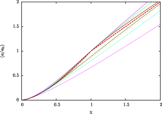
Figure 2: The figure shows the transition function $f(\chi)$, as a function of the dimensionless Ricci scalar $\chi$, for different regimes of gravity, converging to $f(\chi)=\chi$ for $\chi\gg 1$ (general relativity) and to $f(\chi)=\chi^{3/2}$ for $\chi\ll 1$ (a relativistic regime with MOND as its weak field limit) -see equation (37). The thick dash-dot curve is the extreme limiting value $p\to\infty$, i.e. $f(\chi)=\chi^{3/2}$ for $\chi\leq 1$ and $f(\chi)=\chi$ for $\chi\geq 1$. The curves above and below this extreme function represent values of $p=3,\ 2,\ 1,\ 0$ for the minus and plus signs of equation (7) respectively. The extreme limiting curve has a kink at $\chi=1$.

The mass dependence of $\chi$ and $L_{M}$ mean that Hilbert’s action (15) is a function of the mass $M$. This is usually not assumed, since that action is thought to be purely a function of the geometry of space-time due to the presence of mass and energy sources. However, it was Sobouti Sobouti (2007) who first encountered this peculiarity in the Hilbert action when dealing with a metric generalisation of MOND. Following the remarks by Sobouti (2007) and Mendoza and Rosas-Guevara (2007) one should not be surprised if some of the commonly accepted notions, even at the fundamental level of the action, require generalisations and re-thinking. An extended metric theory of gravity goes beyond the traditional general relativity ideas and in this way, we need to change our standard view of its fundamental principles.

4 $F(R,T)$ connection

For the description of gravity shown in section 3 it follows that an adequate way of writing up the gravitational field’s action is given by:

$$S_{\text{f}}=-\frac{c^{3}}{16\pi G}\int{\frac{f(\chi)}{L_{M}^{2}}\sqrt{-g}\,\mathrm{d}^{4}x}.$$ (38)

The function $L_{M}$ is a function of the mass of the system and in general terms it is a function of the space-time coordinates. For the particular case of a spherically symmetric space-time it coincides with the mass of the central object generating the gravitational field as expressed in equations (31) and (33). Generally speaking what the meaning of $M$ would be for a particular distribution of mass and energy needs further research, beyond the scope of this work. Nevertheless one expects that for dust systems with spherically symmetric distributions, the function $M$ would be given by the standard mass-energy relation (see e.g. Misner et al., 1973):

$$M:=\frac{4\pi}{c^{2}}\int{T\,r^{2}\,\mathrm{d}r},$$ (39)

In very general terms, the definition of $M$ in this last equation means that $M$ would not be invariant. However, in some particular systems with high degree of symmetry it is possible to make this quantity invariant. For example, in the case of a spherically symmetric spacetime produced by a point mass that quantity is simply the “Schwarzschild” mass of the point mass generating the gravitational field. In the cosmological case it is also possible to define it as an invariant quantity as discussed in section 5.

The field equations produced by the null variations of the addition of the field’s action $S_{\text{f}}+S_{\text{m}}$ can be constructed in the following form. Harko et al. (2011) have built an $F(R,T)$ theory of gravity, so making the natural identification:

$$F(R,T):=\frac{f(\chi)}{L_{M}^{2}},$$ (40)

it is possible to use all their results for our particular case expressed in equation (40). For example, the null variations of the complete action $S_{\text{f}}+S_{\text{m}}$ for the particular case of equation (40) is given by Harko et al. (2011):

$$\begin{split}\left(\frac{f_{R}}{L_{M}^{2}}\right)\,R_{\mu\nu}-&\frac{1}{2L_{M}^{2}}f\,g_{\mu\nu}+\bigg{[}g_{\mu\nu}\Delta-\nabla_{\mu}\nabla_{\nu}\bigg{]}\left(\frac{f_{R}}{L_{M}^{2}}\right)=\\ &\frac{8\pi G}{c^{4}}T_{\mu\nu}-\left(\frac{f}{L_{M}^{2}}\right)_{T}\bigg{[}T_{\mu\nu}+\Theta_{\mu\nu}\bigg{]},\end{split}$$ (41)

and its trace is given by:

$$\frac{f_{R}\,R}{L_{M}^{2}}-\frac{2f}{L_{M}^{2}}+3\Delta\left(\frac{f_{R}}{L_{M}^{2}}\right)=\frac{8\pi G}{c^{4}}T-\left(\frac{f}{L_{M}^{2}}\right)_{T}\bigg{[}T+\Theta\bigg{]},$$ (42)

where the subscripts $R$ and $T$ stand for the partial derivatives with respect to those quantities, i.e.

$$\bigg{(}\ \ \bigg{)}_{R}:=\frac{\partial}{\partial R},\qquad\text{and}\qquad\bigg{(}\ \ \bigg{)}_{T}:=\frac{\partial}{\partial T}.$$ (43)

The tensor $\Theta_{\mu\nu}$ is such that $\Theta_{\mu\nu}\delta g^{\mu\nu}:=g^{\alpha\beta}\delta T_{\alpha\beta}$ and for the case of an ideal fluid it can be written as (Harko et al., 2011):

$$\Theta_{\mu\nu}=-2T_{\mu\nu}-pg_{\mu\nu}.$$ (44)

Note that equation (41) or (42) converge to the field (18) and trace (20) relations as discussed in section 3 when one considers a point mass generating the gravitational field, i.e. when $L_{M}=\text{const.}$ and so $\partial/\partial R=L_{M}^{2}\partial/\partial\chi$.

In general terms, the $F(R,T)$ theory described by Harko et al. (2011) produces non-geodesic motion of test particles since:

$$\begin{split}\nabla^{\mu}&T_{\mu\nu}=\left(\frac{f}{L_{M}^{2}}\right)_{T}\left\{\frac{8\pi G}{c^{4}}-\left(\frac{f}{L_{M}^{2}}\right)_{T}\right\}^{-1}\times\\ &\left[\left(T_{\mu\nu}+\Theta_{\mu\nu}\right)\nabla^{\mu}\ln\left(\frac{f}{L_{M}^{2}}\right)_{T}\left(R,T\right)+\nabla^{\mu}\Theta_{\mu\nu}\right]\neq 0,\end{split}$$ (45)

and as such the geodesic equation has a force term:

$$\frac{d^{2}x^{\mu}}{ds^{2}}+\Gamma_{\nu\lambda}^{\mu}u^{\nu}u^{\lambda}=\lambda^{\mu},$$ (46)

where the four-force

$$\begin{split}\lambda^{\mu}:=&\frac{8\pi G}{c^{4}}\left(\rho c^{2}+p\right)^{-1}\left[\frac{8\pi G}{c^{4}}+\left(\frac{f}{L_{M}^{2}}\right)_{T}\right]^{-1}\times\\ &\left(g^{\mu\nu}-u^{\mu}u^{\nu}\right)\nabla_{\nu}p,\end{split}$$ (47)

is perpendicular to the four velocity $\mathrm{d}x^{\alpha}/\mathrm{d}s$. As explained by Harko et al. (2011), the motion of test particles is geodesic, i.e. $\lambda^{\mu}=0$ and/or $\nabla^{\alpha}T_{\alpha\beta}=0$, (i) for the case of a pressureless $p=0$ (dust) fluid and (ii) for the cases in which $F_{T}(R,T)=0$.

In what follows we will see how all the previous ideas can be applied to a Friedmann-Lemaître-Robertson-Walker dust universe and so, the divergence of the energy momentum tensor in equation (45) is null. It is worth noting that this condition on the energy-momentum tensor for many applications needs to be zero, including applications to the universe at any epoch.

5 Cosmological applications

There are many good and interesting attempts to explain many cosmological observations using modified theories of gravity (see e.g. Nojiri and Odintsov, 2011, and references therein), however these theories are not generally fully consistent with the gravitational anomalies shown at galactic and extragalactic scales discussed in sections 2 and 3. To see whether the gravitational $f(\chi)$ theory developed in the previous sections can deal with cosmological data, let us now apply the results obtained in those sections to an isotropic Friedmann-Lemaître-Robertson-Walker (FLRW) universe following the procedures first explored by Carranza et al. (2012). In this case, the interval $\mathrm{d}s$ is given by (Longair, 2008):

$$\mathrm{d}s^{2}=c^{2}\mathrm{d}t^{2}-a^{2}(t)\left\{\frac{\mathrm{d}r^{2}}{1-\kappa r^{2}}+r^{2}\mathrm{d}\Omega^{2}\right\},$$ (48)

where $a(t)$ is the scale factor of the universe normalised to unity, i.e. $a_{0}=1$, at the present epoch $t_{0}$, and the angular displacement $\mathrm{d}\Omega^{2}:=\mathrm{d}\theta^{2}+\sin^{2}\theta\,\mathrm{d}\varphi^{2}$ for the polar $\mathrm{d}\theta$ and azimuthal $\mathrm{d}\varphi$ angular displacements with a comoving coordinate distance $r$. In what follows we assume a null space curvature $\kappa=0$ at the present epoch in accordance with observations and deal with the expansion of the universe dictated by the field equations (41), avoiding any form of dark unknown component. Since we are interested on the compatibility of this cosmological model with SNIa observations, in what follows we assume a dust $p=0$ model for which the covariant divergence of the energy-momentum tensor vanishes, and so as discussed in section 4 the trajectories of test particles are geodesic.

To begin with, let us rewrite the field equations (41) inspired by the approach first introduced by Capozziello and Fang (2002) (see also Capozziello and Faraoni (2010)) as follows:

$$G_{\mu\nu}=\frac{8\pi G}{c^{4}}\left\{\left(1+\frac{c^{4}}{8\pi G}F_{T}\right)\frac{T_{\mu\nu}}{F_{R}}+T_{\mu\nu}^{\text{curv}}\right\},$$ (49)

where the Einstein tensor is given by its usual form:

$$G_{\mu\nu}:=R_{\mu\nu}-\frac{1}{2}Rg_{\mu\nu}.$$ (50)

and

$$\begin{split}T_{\mu\nu}^{\text{curv}}:=\frac{c^{4}}{8\pi GF_{R}}&\left[\left(\frac{1}{2}\left(F-RF_{R}\right)-\Delta F_{R}\right)g_{\mu\nu}\right.+\\ &\nabla_{\mu}\nabla_{\nu}F_{R}\bigg{]},\end{split}$$ (51)

represents the “energy-momentum” curvature tensor. Since $T_{00}=\rho c^{2}$, then it will be useful the identification $T_{00}:=\rho_{\text{curv}}c^{2}$. With this last definition and using the fact that the Laplace-Beltrami operator applied to a scalar field $\psi$ is given by (see e.g. Landau and Lifshitz, 1975):

$$\Delta\psi=\frac{1}{\sqrt{-g}}\partial_{\mu}\left(\sqrt{-g}\,g^{\mu\nu}\partial_{\nu}\psi\right),$$ (52)

then

$$\rho_{\text{curv}}=\frac{c^{2}}{8\pi GF_{R}}\left[\frac{1}{2}\left(RF_{R}-F\right)-\frac{3H}{c^{2}}\frac{\mathrm{d}F_{R}}{\mathrm{d}t}\right],$$ (53)

where $H:=\dot{a}(t)/a(t)$ represents Hubble’s constant.

With the above definitions and using the $00$ component of the field’s equations (49) and the relation (cf. Dalarsson and Dalarsson, 2005):

$$R=-\frac{6}{c^{2}}\left[\frac{\ddot{a}}{a}+\left(\frac{\dot{a}}{a}\right)^{2}+\frac{\kappa c^{2}}{a^{2}}\right],$$ (54)

between Ricci’s scalar and the derivatives of the scale factor for a FLRW universe, then the dynamical Friedman’s-like equation for a dust flat universe is:

$$H^{2}=\frac{8\pi G}{3}\left[\left(1+\frac{c^{4}}{8\pi G}F_{T}\right)\frac{\rho}{F_{R}}+\rho_{\text{curv}}\right].$$ (55)

The energy conservation equation is given by the null divergence of the energy-momentum tensor:

$$\left(\frac{8\pi G}{c^{4}}+F_{T}\right)\left(\dot{\rho}+3H\rho\right)=-\rho\frac{\mathrm{d}F_{T}}{\mathrm{d}t}.$$ (56)

For completeness, we write down the correspondent generalisation of Raychadhuri’s equation for a dust flat universe:

$$2\frac{\ddot{a}}{a}+H^{2}=-\frac{8\pi Gp_{\text{curv}}}{c^{2}},$$ (57)

where the “curvature-pressure”

$$p_{\text{curv}}:=\omega c^{2}\rho_{\text{curv}},$$ (58)

and

$$w=\frac{c^{2}\left(F-RF_{R}\right)/2+\mathrm{d}^{2}F_{R}/\mathrm{d}t^{2}+3H\mathrm{d}F_{R}/\mathrm{d}t}{c^{2}\left(RF_{R}-F\right)/2-3H\mathrm{d}F_{R}/\mathrm{d}t}.$$ (59)

On the other hand, note that the mass $M$ that appears on the length $L_{M}$ must be the causally connected mass at a certain cosmic time $t$, since particles beyond Hubble’s (or particle) horizon with respect to a given fundamental observer do not have any gravitational influence on him. At any particular cosmic epoch, this Hubble mass satisfies the spherically symmetric condition implicit in equation (39) and so,

$$M=4\pi\int_{0}^{r_{\text{H}}}{\rho\,r^{2}\,\mathrm{d}r}=\frac{4}{3}\pi\rho\frac{c^{3}}{H^{3}},$$ (60)

where

$$r_{\text{H}}:=\frac{c}{H(t)},$$ (61)

is the Hubble radius or the distance of causal contact at a particular cosmic epoch (Longair, 2008). In this respect the mass $M$ is measured from the point of view of any given fundamental observer at a particular cosmic time $t$ and so, it does not depend on which system of reference (or coordinates) is measured. As such, the mass $M$ represents an invariant scalar quantity. From this last relation it follows that the length (31) is given by:

$$L_{M}=\zeta\frac{\left(\frac{4}{3}\pi c^{3}G\right)^{3/4}}{c\,\mathsf{a}_{0}^{1/4}}\frac{\rho^{3/4}}{H^{9/4}},$$ (62)

and so, by using relation (21) and the standard power-law assumptions:

$$a(t)=a(t_{0})\left(\frac{t}{t_{0}}\right)^{\alpha},\qquad\rho(t)=\rho_{0}\left(\frac{a}{a(t_{0})}\right)^{\beta}.$$ (63)

for the unknown constant powers $\alpha$ and $\beta$, it follows that:

$$\frac{\mathrm{d}F_{R}}{\mathrm{d}t}=b(b-1)R^{b-1}L_{M}^{2(b-1)}H\left[\frac{j-q-2}{1-q}+\frac{3}{2}\left(\beta+\frac{3}{\alpha}\right)\right],$$ (64)

$$\frac{\mathrm{d}F_{T}}{\mathrm{d}t}=\frac{3}{2}(b-1)\frac{R^{b}L_{M}^{2b-2}}{\rho c^{2}},$$ (65)

where

$$q(t):=-\frac{1}{a}\frac{\mathrm{d}^{2}a}{\mathrm{d}t^{2}}H^{-2},\qquad\text{ and }\qquad j:=\frac{1}{a}\frac{\mathrm{d}^{3}a}{\mathrm{d}t^{3}}H^{-3},$$ (66)

are the deceleration parameter and the jerk respectively.

With these and the value of $L_{M}$ from equation (62), the curvature density (53) is given by:

$$\rho_{\text{curv}}=\frac{3H^{2}}{8\pi G}(b-1)\left[\left(1-q\right)-\frac{j-q-2}{1-q}-\frac{3}{2}\left(\beta+\frac{3}{\alpha}\right)\right].$$ (67)

Substitution of the previous relations on Friedmann’s equation (55) gives:

$$H^{2}=\frac{8\pi G\rho}{3\,Z\,F_{R}},$$ (68)

where

$$Z:=1+\left(b-1\right)\left[\frac{j-q-2}{1-q}-\frac{4\left(1-q\right)}{b}+\frac{3}{2}\left(\beta+\frac{3}{\alpha}\right)\right].$$ (69)

is a dimensionless function.

An important result can be obtained evaluating equation (68) at the present epoch, yielding:

$$\mathsf{a}_{0}=\left[\frac{9}{4}\zeta^{4}\left(1-q_{0}\right)^{2}\left(bZ_{0}\right)^{2/\left(b-1\right)}\left(\Omega_{\text{matt}}^{(0)}\right)^{\left(3b-5\right)/\left(b-1\right)}\right]c\,H_{0},$$ (70)

where the density parameter $\Omega_{\text{matt}}^{(0)}$ at the present epoch has been defined by it’s usual relation:

$$\Omega_{\text{matt}}^{(0)}:=\frac{3H^{2}\rho}{8\pi G}.$$ (71)

In other words, the value of Milgrom’s acceleration constant $\mathsf{a}_{0}$ at the current cosmic epoch is such that

$$\mathsf{a}_{0}\approx c\times H_{0}.$$ (72)

The numerical coincidence between the value of Milgrom’s acceleration constant $\mathsf{a}_{0}$ and the multiplication of the speed of light $c$ by the current value of Hubble’s constant $H_{0}$ has been noted since the early development of MOND (see e.g. Famaey and McGaugh, 2011, and references therein). Note that equation (72) means that this coincidence relation occurs at approximately the present cosmic epoch in complete agreement with the results by Bernal, Capozziello, Cristofano and de Laurentis (2011) where it is shown that $\mathsf{a}_{0}$ shows no cosmological evolution and hence it can be postulated as a fundamental constant of nature.

For the power law (21) and the assumptions made above, it follows that the energy conservation equation (56) is given by:

$$\left(\dot{\rho}+3H\rho\right)+\frac{c^{2}}{8\pi G}\left(A\frac{\dot{\rho}}{\rho}+B\,H\right)R^{b}\,L_{M}^{2(b-1)}=0,$$ (73)

where:

$$A:=\frac{9}{4}\left(b-1\right)^{2},$$

$$B:=\frac{9}{2}\frac{b-1}{b}+\frac{27}{4}\frac{\left(b-1\right)^{2}}{\alpha}+\frac{3}{2}\frac{b\left(b-1\right)\left(j-q-2\right)}{1-q}.$$

Direct substitution of the density power law (63) into relation (73) gives a constraint equation between $\alpha$, $\beta$ and $b$:

$$\beta=\frac{1}{\alpha}\left(\frac{9-5b}{3b-5}\right).$$ (74)

Let us now proceed to fix the so far unknown parameters of the theory $\alpha$, $\beta$ and $b$. To do so, we need reliable observational data and as such, we use the redshift-magnitude SNIa data obtained by Riess et al. (2004) and the following well known standard cosmological relations (see e.g. Longair, 2008):

$$1+z=a(t_{0})/a(t),$$ (75)

$$\mu\left(z\right)=5\log_{10}\left[H_{0}\,d_{L}\left(z\right)\right]-5\log_{10}h+42.38,$$ (76)

$$d_{\text{L}}\left(z\right)=\left(1+z\right)\int_{0}^{z}\frac{c}{H\left(z\right)}\,\ \mathrm{d}z,$$ (77)

for the cosmological redshift $z$, the distance modulus $\mu$, the luminosity distance $d_{L}$ and where the normalised Hubble constant $h$ at the present epoch is given by $h:=H_{0}/\left(100\,\mathrm{km}\,\mathrm{s}^{-1}/\,\mathrm{Mpc}\right)$. Also, from equation (63) it follows that

$$H(a)=H_{0}\left(\frac{a}{a(t_{0})}\right)^{-1/\alpha}=H_{0}(1+z)^{1/\alpha},$$ (78)

and the substitution of this into equation (77) gives the distance modulus $d_{L}$ as a function of the redshift $z$. This means that the redshift magnitude relation (76) is a function that depends on the values of the current Hubble constant $H_{0}$ and the value of $\alpha$. Figure 3 shows the best fit to the redshift magnitude relation of SNIa observed by Riess et al. (2004), yielding $\alpha=1.359\pm 0.139$ and $h=0.64\pm 0.009$. The best fit presented on the figure was obtained using the Marquardt-Levenberg fit provided by gnuplot (http://www.gnuplot.info) for non-linear functions. These values do not provide the whole description of the problem, since $\beta$ and $b$ are still unknown. However, according to the constraint equation (74) only one of them is needed in order to know the other once $\alpha$ is known.

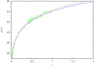
Figure 3: Redshift magnitude plot for SNIa showing the distance modulus $\mu$ as a function of the redshift $z$ for SNIa as presented by Riess et al. (2004). The dotted red line shows the best fit to the data with the $f(\chi)$ gravity theory applied to a flat dust FLRW universe (see text) with no dark components. The continuous blue line represents the best fit according to the standard concordance dust $\Lambda$CDM model.

The parameter $\beta$ can be found from conservation of mass arguments, since the total mass of the universe $M_{\text{tot}}=4\pi\int_{0}^{R_{\text{max}}}{\rho\,r^{2}\,a^{3}\,\mathrm{d}r}=\text{const.}$, where the upper limit of the integral is the radius of the whole universe. Since $a(t)$ and $\rho(t)$ are time dependent functions, the only way the mass of the universe is conserved is by requiring $a^{3}\,\rho=\text{const.}$ and so, $\beta=3$. This argument is exactly the one used in standard cosmology when dealing with a dust FLRW universe (see e.g. Longair, 2008). Using this value of $\beta$ and the one already found for $\alpha$, it follows that $b=1.57\pm 0.56$, which is within the expected value of $b=3/2$ discussed in section 3.

For completeness, we write down a few of the cosmographycal parameters obtained by this $f(\chi)$ gravity applied to the universe:

$$\begin{gathered}h=0.64\pm 0.009,\quad q_{0}=-0.2642\pm 0.075,\\ j_{0}=-0.1246\pm 0.004.\end{gathered}$$ (79)

6 Discussion

As explained by Carranza et al. (2012), the obtained value $b\approx 3/2$ is a completely expected result due to the following arguments. As explained in section 2, a gravitational system for which its characteristic size $r$ is such that $x:=l_{M}/r\lesssim 1$ is in the MONDian gravity regime. For the case of the universe, $x\sim\text{a few}$ and as such if not totally in the MONDian regime of gravity, then it is far away from the regime of Newtonian gravity. The relativistic version of this means that the universe is close to the regime for which $f(\chi)=\chi^{3/2}$ and so $b=3/2$. This is a very important result since seen in this way, the accelerated expansion of the universe is due to an extended gravity theory deviating from general relativity. It is quite interesting to note that the function $f(\chi)=\chi^{3/2}$ which at its non-relativistic limit is capable of predicting the correct dynamical behaviour of many astrophysical phenomena, is also able to explain the behaviour of the current accelerated expansion of the universe.

Seen in this way, the behaviour of gravity towards the past (for sufficiently large redshifts $z$) will differ from $f(\chi)=\chi^{3/2}$ and eventually converge to $f(\chi)=\chi$, i.e. the gravitational regime of gravity is general relativity for sufficiently large redshifts. A very detailed investigation into this needs to be done at different levels in order to be coherent many different cosmological observations (see e.g. Longair, 2011). This in turn can serve to calibrate the index $p$ of the transfer function $f(\chi)$ as presented in equation (37), which has a very soft transition when $p=-1$, i.e.,

$$f(\chi)=\frac{\chi^{3/2}}{1+\chi^{3/2}},$$ (80)

and also has a very sharp transition when $p\rightarrow\infty$, with the step function:

$$f(\chi)=\begin{cases}\chi^{3/2},\quad\text{for }0\leq\chi\leq 1,\\ \chi,\qquad\ \text{for }\chi\geq 1.\end{cases}$$ (81)

In this respect, perhaps something close to a sharp transition (81) will be observed since, as mentioned in section 2, at the non-relativistic level different astrophysical observations show a sharp transition from the Newtonian to the MONDian regimes. This sort of decision has to be taken with care and such a full description requires to analyse in full detail the whole Friedmann-like equations:

$$\begin{split}\left(\frac{8\pi G}{c^{4}}+F_{T}\right)&\left(\dot{\rho}+3H\rho+\frac{3Hp}{c^{2}}\right)=\\ &-\rho\frac{\mathrm{d}F_{T}}{\mathrm{d}t}+\frac{1}{c^{2}}\left(p\frac{\mathrm{d}F_{T}}{\mathrm{d}t}+F_{T}\frac{\mathrm{d}p}{\mathrm{d}t}\right),\end{split}$$ (82)

$$H^{2}=\frac{8\pi G}{3}\left[\left(1+\frac{c^{4}F_{T}}{8\pi G}\right)\frac{\rho}{F_{R}}+\rho_{\text{curv}}\right]-\frac{\kappa c^{2}}{a^{2}},$$ (83)

$$2\frac{\ddot{a}}{a}+H^{2}+\frac{\kappa c^{2}}{a^{2}}=-\frac{8\pi Gp}{c^{2}F_{R}}-\frac{2pc^{2}F_{T}}{F_{R}}-\frac{8\pi Gp_{\text{curv}}}{c^{2}}.$$ (84)

These equations are directly obtained from taking the null covariant divergence of the energy momentum tensor, the $00$ component of the field equations (49) and the density $\rho$ contains all species of matter and/or radiation. The curvature density $\rho_{\text{curv}}$ and the curvature pressure $p_{\text{curv}}$ are related to one another by relation (58) with $\omega$ given by equation (59).

It is quite remarkable that a metric extended theory of gravity is able to reproduce phenomena from mass and length scales associated to the solar system up to cosmological scales. There are many more astrophysical challenges that this theory needs to address, in particular with respect to lensing at different scales and the dynamics associated to galaxy clusters. These will be addressed elsewhere.

7 Acknowledgements

This work was supported by a DGAPA-UNAM grant (PAPIIT IN116210-3) and CONACyT 26344. The author acknowledges fruitful discussions at different stages with Tula Bernal, Diego Carranza, Salvatore Capozziello, Rituparno Goswami, Xavier Hernandez, Juan Carlos Hidalgo and Luis Torres.

References

- (1)
- Bekenstein (2006a) Bekenstein, J. (2006a). The modified Newtonian dynamics - MOND and its implications for new physics, Contemporary Physics 47: 387–403.
- Bekenstein (2006b) Bekenstein, J. (2006b). The modified Newtonian dynamics - MOND and its implications for new physics, Contemporary Physics 47: 387–403.
- Bekenstein (2004) Bekenstein, J. D. (2004). Relativistic gravitation theory for the modified Newtonian dynamics paradigm, Phys. Rev. D 70(8): 083509.
- Bernal, Capozziello, Cristofano and de Laurentis (2011) Bernal, T., Capozziello, S., Cristofano, G. and de Laurentis, M. (2011). Mond’s Acceleration Scale as a Fundamental Quantity, Modern Physics Letters A 26: 2677–2687.
- Bernal, Capozziello, Hidalgo and Mendoza (2011) Bernal, T., Capozziello, S., Hidalgo, J. C. and Mendoza, S. (2011). Recovering MOND from extended metric theories of gravity, European Physical Journal C 71: 1794.
- Blanchet and Marsat (2012) Blanchet, L. and Marsat, S. (2012). Relativistic MOND theory based on the Khronon scalar field, ArXiv e-prints .
- Capozziello et al. (2010) Capozziello, S., de Laurentis, M. and Faraoni, V. (2010). A Bird’s Eye View of f(R)-Gravity, The Open Astronomy Journal 3: 49–72.
- Capozziello and Fang (2002) Capozziello, S. and Fang, L. Z. (2002). Curvature Quintessence, International Journal of Modern Physics D 11: 483–491.
- Capozziello and Faraoni (2010) Capozziello, S. and Faraoni, V. (2010). Beyond Einstein Gravity: A Survey of Gravitational Theories for Cosmology and Astrophysics, Fundamental Theories of Physics, Springer.
- Carranza et al. (2012) Carranza, D. A., Mendoza, S. and Torres, L. A. (2012). A cosmological dust model with extended gravity, ArXiv e-prints .
- Dalarsson and Dalarsson (2005) Dalarsson, M. and Dalarsson, N. (2005). Tensor calculus, relativity, and cosmology : a first course.
- Exirifard (2011) Exirifard, Q. (2011). Lunar system constraints on the modified theories of gravity, ArXiv e-prints .
- Famaey and McGaugh (2011) Famaey, B. and McGaugh, S. (2011). Modified Newtonian Dynamics (MOND): Observational Phenomenology and Relativistic Extensions, ArXiv e-prints .
- Harko et al. (2011) Harko, T., Lobo, F. S. N., Nojiri, S. and Odintsov, S. D. (2011). f(R,T) gravity, Phys. Rev. D 84(2): 024020.
- Hernandez and Jiménez (2012) Hernandez, X. and Jiménez, M. A. (2012). The Outskirts of Globular Clusters as Modified Gravity Probes, ApJ 750: 9.
- Hernandez et al. (2012a) Hernandez, X., Jimenez, M. A. and Allen, C. (2012a). Flattened velocity dispersion profiles in Globular Clusters: Newtonian tides or modified gravity?, ArXiv e-prints .
- Hernandez et al. (2012b) Hernandez, X., Jiménez, M. A. and Allen, C. (2012b). Wide binaries as a critical test of classical gravity, European Physical Journal C 72: 1884.
- Hernandez et al. (2010) Hernandez, X., Mendoza, S., Suarez, T. and Bernal, T. (2010). Understanding local dwarf spheroidals and their scaling relations under MOdified Newtonian Dynamics, A&A 514: A101.
- Landau and Lifshitz (1975) Landau, L. and Lifshitz, E. (1975). The classical theory of fields, Course of theoretical physics, Butterworth Heinemann.
- Longair (2011) Longair, M. (2011). The Frontiers of Observational Cosmology and the Confrontation with Theory, Journal of Physics Conference Series 314(1): 012011.
- Longair (2008) Longair, M. S. (2008). Galaxy Formation.
- Mendoza et al. (2012) Mendoza, S., Bernal, T., Hernandez, X., Hidalgo, J. C. and Torres, L. A. (2012). Gravitational lensing with gravity in accordance with astrophysical observations, ArXiv e-prints .
- Mendoza et al. (2011) Mendoza, S., Hernandez, X., Hidalgo, J. C. and Bernal, T. (2011). A natural approach to extended Newtonian gravity: tests and predictions across astrophysical scales, MNRAS 411: 226–234.
- Mendoza and Rosas-Guevara (2007) Mendoza, S. and Rosas-Guevara, Y. M. (2007). Gravitational waves and lensing of the metric theory proposed by Sobouti, A&A 472: 367–371.
- Meyer et al. (2011) Meyer, H., Lohrmann, E., Schubert, S., Bartel, W., Glazov, A., Loehr, B., Niebuhr, C., Wuensch, E., Joensson, L. and Kempf, G. (2011). Test of the Law of Gravitation at small Accelerations, ArXiv e-prints .
- Milgrom (1983) Milgrom, M. (1983). A modification of the Newtonian dynamics - Implications for galaxies, ApJ 270: 371–389.
- Milgrom (2008) Milgrom, M. (2008). The MOND paradigm, arXiv:0801.3133 .
- Milgrom (2009) Milgrom, M. (2009). New Physics at Low Accelerations (MOND): an Alternative to Dark Matter, arXiv:0912.2678 .
- Milgrom (2010) Milgrom, M. (2010). New Physics at Low Accelerations (MOND): an Alternative to Dark Matter, in J.-M. Alimi & A. Fuözfa (ed.), American Institute of Physics Conference Series, Vol. 1241 of American Institute of Physics Conference Series, pp. 139–153.
- Mishra and Singh (2012) Mishra, P. and Singh, T. P. (2012). Galaxy rotation curves from a fourth order gravity, ArXiv e-prints .
- Misner et al. (1973) Misner, C. W., Thorne, K. S. and Wheeler, J. A. (1973). Gravitation, San Francisco: W.H. Freeman and Co., 1973.
- Nojiri and Odintsov (2011) Nojiri, S. and Odintsov, S. D. (2011). Unified cosmic history in modified gravity: From F(R) theory to Lorentz non-invariant models, Phys. Rep. 505: 59–144.
- Puech et al. (2010) Puech, M., Hammer, F., Flores, H., Delgado-Serrano, R., Rodrigues, M. and Yang, Y. (2010). The baryonic content and Tully-Fisher relation at z ~ 0.6, A&A 510: A68+.
- Riess et al. (2004) Riess, A. G., Strolger, L.-G., Tonry, J., Casertano, S., Ferguson, H. C., Mobasher, B., Challis, P., Filippenko, A. V., Jha, S., Li, W., Chornock, R., Kirshner, R. P., Leibundgut, B., Dickinson, M., Livio, M., Giavalisco, M., Steidel, C. C., Benítez, T. and Tsvetanov, Z. (2004). Type Ia Supernova Discoveries at z from the Hubble Space Telescope: Evidence for Past Deceleration and Constraints on Dark Energy Evolution, ApJ 607: 665–687.
- Sedov (1959) Sedov, L. I. (1959). Similarity and Dimensional Methods in Mechanics, Academic Press.
- Sobouti (2007) Sobouti, Y. (2007). An f(R) gravitation for galactic environments, A&A 464: 921–925.
- Sotiriou and Faraoni (2010) Sotiriou, T. P. and Faraoni, V. (2010). f(R) theories of gravity, Reviews of Modern Physics 82: 451–497.