Let $P$ be a set of $n$ points in ${\mathbb{R}}^{d}$. We present a linear-size data structure for answering range queries on $P$ with constant-complexity semialgebraic sets as ranges, in time close to $O(n^{1-1/d})$. It essentially matches the performance of similar structures for simplex range searching, and, for $d\geq 5$, significantly improves earlier solutions by the first two authors obtained in 1994. This almost settles a long-standing open problem in range searching.

The data structure is based on the polynomial-partitioning technique of Guth and Katz [arXiv:1011.4105], which shows that for a parameter $r$, $1<r\leq n$, there exists a $d$-variate polynomial $f$ of degree $O(r^{1/d})$ such that each connected component of ${\mathbb{R}}^{d}\setminus Z(f)$ contains at most $n/r$ points of $P$, where $Z(f)$ is the zero set of $f$. We present an efficient randomized algorithm for computing such a polynomial partition, which is of independent interest and is likely to have additional applications.

1 Introduction

Range searching.

Let $P$ be a set of $n$ points in ${\mathbb{R}}^{d}$, where $d$ is a small constant. Let $\Gamma$ be a family of geometric “regions,” called ranges, in ${\mathbb{R}}^{d}$, each of which can be described algebraically by some fixed number of real parameters (a more precise definition is given below). For example, $\Gamma$ can be the set of all axis-parallel boxes, balls, simplices, or cylinders, or the set of all intersections of pairs of ellipsoids. In the $\Gamma$-range searching problem, we want to preprocess $P$ into a data structure so that the number of points of $P$ lying in a query range $\gamma\in\Gamma$ can be counted efficiently. Similar to many previous papers, we actually consider a more general setting, the so-called semigroup model, where we are given a weight function on the points in $P$ and we ask for the cumulative weight of the points in $P\cap\gamma$. The weights are assumed to belong to a semigroup, i.e., subtractions are not allowed. We assume that the semigroup operation can be executed in constant time.

In this paper we consider the case in which $\Gamma$ is a set of constant-complexity semialgebraic sets. We recall that a semialgebraic set is a subset of ${\mathbb{R}}^{d}$ obtained from a finite number of sets of the form $\{x\in{\mathbb{R}}^{d}\mid g(x)\geq 0\}$, where $g$ is a $d$-variate polynomial with integer coefficients, by Boolean operations (unions, intersections, and complementations). Specifically, let $\Gamma_{d,\Delta,s}$ denote the family of all semialgebraic sets in ${\mathbb{R}}^{d}$ defined by at most $s$ polynomial inequalities of degree at most $\Delta$ each. If $d,\Delta,s$ are all regarded as constants, we refer to the sets in $\Gamma_{d,\Delta,s}$ as constant-complexity semialgebraic sets (such sets are sometimes also called Tarski cells). By semialgebraic range searching we mean $\Gamma_{d,\Delta,s}$-range searching for some parameters $d,\Delta,s$; in most applications the actual collection $\Gamma$ of ranges is only a restricted subset of some $\Gamma_{d,\Delta,s}$. Besides being interesting in its own right, semialgebraic range searching also arises in several geometric searching problems, such as searching for a point nearest to a query geometric object, counting the number of input objects intersecting a query object, and many others.

This paper focuses on the low storage version of range searching with constant-complexity semialgebraic sets—the data structure is allowed to use only linear or near-linear storage, and the goal is to make the query time as small as possible. At the other end of the spectrum we have the fast query version, where we want queries to be answered in polylogarithmic time using as little storage as possible. This variant is discussed briefly in Section 8.

As is typical in computational geometry, we will use the real RAM model of computation, where we can compute exactly with arbitrary real numbers and each arithmetic operation is executed in constant time.

Previous work.

Motivated by a wide range of applications, several variants of range searching have been studied in computational geometry and database systems at least since the 1980s. See [1, 23] for comprehensive surveys of this topic. The early work focused on the so-called orthogonal range searching, where ranges are axis-parallel boxes. After three decades of extensive work on this particular case, some basic questions still remain open. However, geometry plays little role in the known data structures for orthogonal range searching.

The most basic and most studied truly geometric instance of range searching is with halfspaces, or more generally simplices, as ranges. Studies in the early 1990s have essentially determined the optimal trade-off between the worst-case query time and the storage (and preprocessing time) required by any data structure for simplex range searching. Lower bounds for this trade-off have been given by Chazelle [7] under the semigroup model of computation, where subtraction of the point weights is not allowed. It is possible that, say, the counting version of the simplex range searching problem, where we ask just for the number of points in the query simplex, might admit better solutions using subtractions, but no such solutions are known. Moreover, there are recent lower-bound results when subtractions are also allowed; see [19] and references therein.

The data structures proposed for simplex range searching over the last two decades [21, 22] match the known lower bounds within polylogarithmic factors. The state-of-the-art upper bounds are by (i) Chan [6], who, building on many earlier results, provides a linear-size data structure with $O(n\log n)$ expected preprocessing time and $O(n^{1-1/d})$ query time, and (ii) Matoušek [22], who provides a data structure with $O(n^{d})$ storage, $O((\log n)^{d+1})$ query time, and $O(n^{d}(\log n)^{\varepsilon})$ preprocessing time. A trade-off between space and query time can be obtained by combining these two data structures [22].

Yao and Yao [32] were perhaps the first to consider range searching in which ranges were delimited by graphs of polynomial functions. Agarwal and Matoušek [2] have introduced a systematic study of semialgebraic range searching. Building on the techniques developed for simplex range searching, they presented a linear-size data structure with $O(n^{1-1/b+\varepsilon})$ query time, where $b=\max(d,2d-4)$. For $d\leq 4$, this almost matches the performance for the simplex range searching, but for $d\geq 5$ there is a gap in the exponents of the corresponding bounds. Also see [28] for related recent developments.

The bottleneck in the performance of the just mentioned range-searching data structure of [2] is a combinatorial geometry problem, known as the decomposition of arrangements into constant-complexity cells. Here, we are given a set $\Sigma$ of $t$ algebraic surfaces in ${\mathbb{R}}^{d}$ (i.e., zero sets of $d$-variate polynomials), with degrees bounded by a constant $\Delta_{0}$, and we want to decompose each cell of the arrangement $\mathcal{A}(\Sigma)$ (see Section 4 for details) into subcells that are constant-complexity semialgebraic sets, i.e., belong to $\Gamma_{d,\Delta,s}$ for some constants $\Delta$ (bound on degrees) and $s$ (number of defining polynomials), which may depend on $d$ and $\Delta_{0}$, but not on $t$. The crucial quantity is the total number of the resulting subcells over all cells of $\mathcal{A}(\Sigma)$; namely, if one can construct such a decomposition with $O(t^{b})$ subcells, with some constant $b$, for every $t$ and $\Sigma$, then the method of [2] yields query time $O(n^{1-1/b+\varepsilon})$ (with linear storage). The only known general-purpose technique for producing such a decomposition is the so-called vertical decomposition [8, 27], which decomposes $\mathcal{A}(\Sigma)$ into roughly $t^{2d-4}$ constant-complexity subcells, for $d\geq 4$ [18, 27].

An alternative approach, based on linearization, was also proposed in [2]. It maps the semialgebraic ranges in ${\mathbb{R}}^{d}$ to simplices in some higher-dimensional space and uses simplex range searching there. However, its performance depends on the specific form of the polynomials defining the ranges. In some special cases (e.g., when ranges are balls in ${\mathbb{R}}^{d}$), linearization yields better query time than the decomposition-based technique mentioned above, but for general constant-complexity semialgebraic ranges, linearization has worse performance.

Our results.

In a recent breakthrough, Guth and Katz [12] have presented a new space decomposition technique, called polynomial partitioning. For a set $P\subset{\mathbb{R}}^{d}$ of $n$ points and a real parameter $r$, $1<r\leq n$, an $r$-partitioning polynomial for $P$ is a nonzero $d$-variate polynomial $f$ such that each connected component of ${\mathbb{R}}^{d}\setminus Z(f)$ contains at most $n/r$ points of $P$, where $Z(f):=\{x\in{\mathbb{R}}^{d}\mid f(x)=0\}$ denotes the zero set of $f$. The decomposition of ${\mathbb{R}}^{d}$ into $Z(f)$ and the connected components of ${\mathbb{R}}^{d}\setminus Z(f)$ is called a polynomial partition (induced by $f$). Guth and Katz show that an $r$-partitioning polynomial of degree $O(r^{1/d})$ always exists, but their argument does not lead to an efficient algorithm for constructing such a polynomial, mainly because it relies on ham-sandwich cuts in high-dimensional spaces, for which no efficient construction is known. Our first result is an efficient randomized algorithm for computing an $r$-partitioning polynomial.

Theorem 1.1.

Given a set $P$ of $n$ points in ${\mathbb{R}}^{d}$, for some fixed $d$, and a parameter $r\leq n$, an $r$-partitioning polynomial for $P$ of degree $O(r^{1/d})$ can be computed in randomized expected time $O(nr+r^{3})$.

Next, we use this algorithm to bypass the arrangement-decomposition problem mentioned above. Namely, based on polynomial partitions, we construct partition trees [1, 23] that answer range queries with constant-complexity semialgebraic sets in near-optimal time, using linear storage. An essential ingredient in the performance analysis of these partition trees is a recent combinatorial result of Barone and Basu [3], originally conjectured by the second author, which deals with the complexity of certain kinds of arrangements of zero sets of polynomials (see Theorem 4.2). While there have already been several combinatorial applications of the Guth-Katz technique (the most impressive being the original one in [12], which solves the famous Erdős’s distinct distances problem, and some of the others presented in [14, 15, 29, 34]), ours seems to be the first algorithmic application.

We establish two range-searching results, both based on polynomial partitions. For the first result, we need to introduce the notion of $D$-general position, for an integer $D\geq 1$. We say that a set $P\subset{\mathbb{R}}^{d}$ is in $D$-general position if no $k$ points of $P$ are contained in the zero set of a nonzero $d$-variate polynomial of degree at most $D$, where $k:={D+d\choose d}$. This is the number one expects for a “generic” point set.

Theorem 1.2.

Let $d,\Delta,s$ and $\varepsilon>0$ be constants. Let $P\subset{\mathbb{R}}^{d}$ be an $n$-point set in $D_{0}$-general position, where $D_{0}$ is a suitable constant depending on $d,\Delta$, and $\varepsilon$. Then the $\Gamma_{d,\Delta,s}$-range searching problem for $P$ can be solved with $O(n)$ storage, $O(n\log n)$ expected preprocessing time, and $O(n^{1-1/d+\varepsilon})$ query time.

We note that both here and in the next theorem, while the preprocessing algorithm is randomized, the queries are answered deterministically, and the query time bound is worst-case.

Of course, we would like to handle arbitrary point sets, not only those in $D_{0}$-general position. This can be achieved by an infinitesimal perturbation of the points of $P$. A general technique known as “simulation of simplicity” (in the version considered by Yap [33]) ensures that the perturbed set $P^{\prime}$ is in $D_{0}$-general position. If a point $p\in P$ lies in the interior of a query range $\gamma$, then so does the corresponding perturbed point $p^{\prime}\in P^{\prime}$, and similarly for $p$ in the interior of ${\mathbb{R}}^{d}\setminus\gamma$. However, for $p$ on the boundary of $\gamma$, we cannot be sure if $p^{\prime}$ ends up inside or outside $\gamma$.

Let us say that a boundary-fuzzy solution to the $\Gamma_{d,\Delta,s}$-range searching problem is a data structure that, given a query $\gamma\in\Gamma_{d,\Delta,s}$, returns an answer in which all points of $P$ in the interior of $\gamma$ are counted and none in the interior of ${\mathbb{R}}^{d}\setminus\gamma$ is counted, while each point $p\in P$ on the boundary of $\gamma$ may or may not be counted. In some applications, we can think of the points of $P$ being imprecise anyway (e.g., their coordinates come from some imprecise measurement), and then boundary-fuzzy range searching may be adequate.

Corollary 1.3.

Let $d,\Delta,s$, and $\varepsilon>0$ be constants. Then for every $n$-point set in ${\mathbb{R}}^{d}$, there is a boundary-fuzzy $\Gamma_{d,\Delta,s}$-range searching data structure with $O(n)$ storage, $O(n\log n)$ expected preprocessing time, and $O(n^{1-1/d+\varepsilon})$ query time.

Actually, previous results on range searching that use simulation of simplicity to avoid degenerate cases also solve only the boundary-fuzzy variant (see e.g. [21, 22]). However, the previous techniques, even if presented only for point sets in general position, can usually be adapted to handle degenerate cases as well, perhaps with some effort, which is nevertheless routine. For our technique, degeneracy appears to be a more substantial problem because it is possible that a large subset of $P$ (maybe even all of $P$) is contained in the zero set of the partitioning polynomial $f$, and the recursive divide-and-conquer mechanism yielded by the partition of $f$ does not apply to this subset.

Partially in response to this issue, we present a different data structure that, at a somewhat higher preprocessing cost, not only gets rid of the boundary-fuzziness condition but also has a slightly improved query time (in terms of $n$). The main idea is that we build an auxiliary recursive data structure to handle the potentially large subset of points that lie in the zero set of the partitioning polynomial.

Theorem 1.4.

Let $d,\Delta,s$, and $\varepsilon>0$ be constants. Then the $\Gamma_{d,\Delta,s}$-range searching problem for an arbitrary $n$-point set in ${\mathbb{R}}^{d}$ can be solved with $O(n)$ storage, $O(n^{1+\varepsilon})$ expected preprocessing time, and $O(n^{1-1/d}\log^{B}n)$ query time, where $B$ is a constant depending on $d,\Delta,s$ and $\varepsilon$.

We remark that the dependence of $B$ on $\Delta$, $s$, and $\varepsilon$ is reasonable, but its dependence on $d$ is superexponential.

Our algorithms work for the semigroup model described earlier. Assuming that a semigroup operation can be executed in constant time, the query time remains the same as for the counting query. A reporting query—report the points of $P$ lying in a query range—also fits in the semigroup model, except one cannot assume that a semigroup operation in this case takes constant time. The time taken by a reporting query is proportional to the cost of a counting query plus the number of reported points.

Roadmap of the paper.

Our algorithm is based on the polynomial partitioning technique by Guth and Katz, and we begin by briefly reviewing it in Section 2. Next, in Section 3, we describe the randomized algorithm for constructing such a partitioning polynomial. Section 4 presents an algorithm for computing the cells of a polynomial partition that are crossed by a semialgebraic range, and discusses several related topics. Section 5 presents our first data structure, which is as in Theorem 1.2. Section 6 describes the method for handling points lying on the zero set of the partitioning polynomial, and Section 7 presents our second data structure. We conclude in Section 8 by mentioning a few open problems.

2 Polynomial Partitions

In this section we briefly review the Guth-Katz technique for later use. We begin by stating their result.

Theorem 2.1 (Guth-Katz [12]).

Given a set $P$ of $n$ points in ${\mathbb{R}}^{d}$ and a parameter $r\leq n$, there exists an $r$-partitioning polynomial for $P$ of degree at most $O(r^{1/d})$ (for $d$ fixed).

The degree in the theorem is asymptotically optimal in the worst case because the number of connected components of ${\mathbb{R}}^{d}\setminus Z(f)$ is $O((\deg f)^{d})$ for every polynomial $f$ (see, e.g., Warren [31, Theorem 2]).

• The Guth-Katz proof uses the polynomial ham sandwich theorem of Stone and Tukey [30], which we state here in a version for finite point sets: If $A_{1},\ldots,A_{k}$ are finite sets in ${\mathbb{R}}^{d}$ and $D$ is an integer satisfying ${D+d\choose d}-1\geq k$, then there exists a nonzero polynomial $f$ of degree at most $D$ that simultaneously bisects all the sets $A_{i}$. Here “$f$ bisects $A_{i}$” means that $f>0$ in at most $\lfloor|A_{i}|/2\rfloor$ points of $A_{i}$ and $f<0$ in at most $\lfloor|A_{i}|/2\rfloor$ points of $A_{i}$; $f$ might vanish at any number of the points of $A_{i}$, possibly even at all of them.

  Guth and Katz inductively construct collections $\mathcal{P}_{0},\mathcal{P}_{1},\ldots,\mathcal{P}_{m}$ of subsets of $P$. For $j=0,1,\ldots,m$, $\mathcal{P}_{j}$ consists of at most $2^{j}$ pairwise-disjoint subsets of $P$, each of size at most $n/2^{j}$; the union of these sets does not have to contain all points of $P$.

  Initially, we have $\mathcal{P}_{0}=\{P\}$. The algorithm stops as soon as each subset in $\mathcal{P}_{m}$ has at most $n/r$ points. This implies that $m\leq\lceil\log_{2}r\rceil$. Having constructed $\mathcal{P}_{j-1}$, we use the polynomial ham-sandwich theorem to construct a polynomial $f_{j}$ that bisects each set of $\mathcal{P}_{j-1}$, with $\deg f_{j}=O(2^{j/d})$ (this is indeed an asymptotic upper bound for the smallest $D$ satisfying ${D+d\choose d}-1\geq 2^{j-1}$, assuming $d$ to be a constant). For every subset $Q\in\mathcal{P}_{j-1}$, let $Q^{+}=\{q\in Q\mid f_{j}(q)>0\}$ and $Q^{-}=\{q\in Q\mid f_{j}(q)<0\}$. We set $\mathcal{P}_{j}:=\{Q^{+},Q^{-}\mid Q\in\mathcal{P}_{j-1}\}$; empty subsets are not included in $\mathcal{P}_{j}$.

  The desired $r$-partitioning polynomial for $P$ is then the product $f:=f_{1}f_{2}\cdots f_{m}$. We have

  $$\deg f=\sum_{j=1}^{m}\deg f_{j}=\sum_{j=1}^{m}O(2^{j/d})=O(r^{1/d}).$$

  By construction, the points of $P$ lying in a single connected component of ${\mathbb{R}}^{d}\setminus Z(f)$ belong to a single member of $\mathcal{P}_{m}$, which implies that each connected component contains at most $n/r$ points of $P$. ∎

• We begin by observing that ${D+d\choose d}-1$ is the number of all nonconstant monomials of degree at most $D$ in $d$ variables. Thus, we fix a collection ${\mathcal{M}}$ of $k\leq{D+d\choose d}-1$ such monomials. Let $\Phi\colon{\mathbb{R}}^{d}\to{\mathbb{R}}^{k}$ be the corresponding Veronese map, which maps a point $x=(x_{1},\ldots,x_{d})\in{\mathbb{R}}^{d}$ to the $k$-tuple of the values at $(x_{1},\ldots,x_{d})$ of the monomials from ${\mathcal{M}}$. For example, for $d=2$, $D=3$, and $k=8\leq{3+2\choose 2}-1$, we may use $\Phi(x_{1},x_{2})=(x_{1},x_{2},x_{1}^{2},x_{1}x_{2},x_{2}^{2},x_{1}^{3},x_{1}^{2}x_{2},x_{1}x_{2}^{2})\in{\mathbb{R}}^{8}$, where ${\mathcal{M}}$ is the set of the eight monomials appearing as components of $\Phi$.

  Let $B_{i}:=\Phi(A_{i})\subset{\mathbb{R}}^{k}$ be the image of the given $A_{i}$ under this Veronese map, for $i=1,\ldots,k$. By the standard ham-sandwich theorem (see, e.g., [24]), there exists a hyperplane $h$ in ${\mathbb{R}}^{k}$ that simultaneously bisects all the $B_{i}$’s, in the sense that each open halfspace bounded by $h$ contains at most half of the points of each of the sets $B_{i}$. In a more algebraic language, there is a nonzero $k$-variate linear polynomial, which we also call $h$, that bisects all the $B_{i}$’s, in the sense of being positive on at most half of the points of each $B_{i}$, and being negative on at most half of the points of each $B_{i}$. Then $f:=h\circ\Phi$ is the desired $d$-variate polynomial of degree at most $D$ bisecting all the $A_{i}$’s. ∎

3 Constructing a Partitioning Polynomial

In this section we present an efficient randomized algorithm that, given a point set $P$ and a parameter $r<n$, constructs an $r$-partitioning polynomial. The main difficulty in converting the above proof of the Guth-Katz partitioning theorem into an efficient algorithm is the use of the ham-sandwich theorem in the possibly high-dimensional space ${\mathbb{R}}^{k}$. A straightforward algorithm for computing ham-sandwich cuts in ${\mathbb{R}}^{k}$ inspects all possible ways of splitting the input point sets by a hyperplane, and has running time about $n^{k}$. Compared to this easy upper bound, the best known ham-sandwich algorithms can save a factor of about $n$ [20], but this is insignificant in higher dimensions. A recent result of Knauer, Tiwari, and Werner [17] shows that a certain incremental variant of computing a ham-sandwich cut is $W[1]$-hard (where the parameter is the dimension), and thus one perhaps should not expect much better exact algorithms.

We observe that the exact bisection of each $A_{i}$ is not needed in the Guth-Katz construction—it is sufficient to replace the Stone–Tukey polynomial ham-sandwich theorem by a weaker result, as described below.

Constructing a well-dissecting polynomial.

We say that a polynomial $f$ is well-dissecting for a point set $A$ if $f>0$ on at most $\frac{7}{8}|A|$ points of $A$ and $f<0$ on at most $\frac{7}{8}|A|$ points of $A$. Given point sets $A_{1},\ldots,A_{k}$ in ${\mathbb{R}}^{d}$ with $n$ points in total, we present a Las-Vegas algorithm for constructing a polynomial $f$ of degree $O(k^{1/d})$ that is well-dissecting for at least $\lceil k/2\rceil$ of the $A_{i}$’s.

As in the above proof of the Stone–Tukey polynomial ham-sandwich theorem, let $D$ be the smallest integer satisfying ${D+d\choose d}-1\geq k$. We fix a collection ${\mathcal{M}}$ of $k$ distinct nonconstant monomials of degree at most $D$, and let $\Phi$ be the corresponding Veronese map. For each $i=1,2,\ldots,k$, we pick a point $a_{i}\in A_{i}$ uniformly at random and compute $b_{i}:=\Phi(a_{i})$. Let $h$ be a hyperplane in ${\mathbb{R}}^{k}$ passing through $b_{1},\ldots,b_{k}$, which can be found by solving a system of linear equations, in $O(k^{3})$ time.

If the points $b_{1},\ldots,b_{k}$ are not affinely independent, then $h$ is not determined uniquely (this is a technical nuisance, which the reader may want to ignore on first reading). In order to handle this case, we prepare in advance, before picking the $a_{i}$’s, auxiliary affinely independent points $q_{1},\ldots,q_{k}$ in ${\mathbb{R}}^{k}$, which are in general position with respect to $\Phi(A_{1}),\ldots,\Phi(A_{k})$; here we mean the “ordinary” general position, i.e., no unnecessary affine dependences, that involve some of the $q_{i}$’s and the other points, arise. The points $q_{i}$ can be chosen at random, say, uniformly in the unit cube; with high probability, they have the desired general position property. (If we do not want to assume the capability of choosing a random real number, we can pick the $q_{i}$’s uniformly at random from a sufficiently large discrete set.) If the dimension of the affine hull of $b_{1},\ldots,b_{k}$ is $k^{\prime}<k-1$, we choose the hyperplane $h$ through $b_{1},\ldots,b_{k}$ and $q_{1},\ldots,q_{k-k^{\prime}-1}$. If $h$ is not unique, i.e., $q_{1},\ldots q_{k-k^{\prime}-1}$ are not affinely independent with respect to $b_{1},\ldots b_{k}$, which we can detect while solving the linear system, we restart the algorithm by choosing $q_{1},\ldots,q_{k}$ anew and then picking new $a_{1},\ldots,a_{k}$. In this way, after a constant expected number of iterations, we obtain the uniquely determined hyperplane $h$ through $b_{1},\ldots,b_{k}$ and $q_{1},\ldots,q_{k-k^{\prime}-1}$ as above, and we let $f=h\circ\Phi$ denote the corresponding $d$-variate polynomial. We refer to these steps as one trial of the algorithm. For each $A_{i}$, we check whether $f$ is well-dissecting for $A_{i}$. If $f$ is well-dissecting for only fewer than $k/2$ sets, then we discard $f$ and perform another trial.

We now analyze the expected running time of the algorithm. The intuition is that $f$ is expected to well-dissect a significant fraction, say at least half, of the sets $A_{i}$. This intuition is reflected in the next lemma. Let $X_{i}$ be the indicator variable of the event: $A_{i}$ is not well-dissected by $f$.

Lemma 3.1.

For every $i=1,2,\ldots,k$, ${\mathbb{E}}[X_{i}]\leq 1/4$.

• Let us fix $i$ and the choices of $a_{j}$ (and thus of $b_{j}=\Phi(a_{j})$) for all $j\neq i$. Let $k_{0}$ be the dimension of $F_{0}$, the affine hull of $\{b_{j}\mid j\neq i\}$. Then the resulting hyperplane $h$ passes through the $(k-2)$-flat $F$ spanned by $F_{0}$ and $q_{1},\ldots,q_{k-k_{0}-2}$, irrespective of which point of $A_{i}$ is chosen. If $a_{i}$, the point chosen from $A_{i}$, is such that $b_{i}=\Phi(a_{i})$ lies on $F_{0}$, then $h$ also passes through $q_{k-k_{0}-1}$.

  Put $B_{i}:=\Phi(A_{i})$, and let us project the configuration orthogonally to a 2-dimensional plane $\pi$ orthogonal to $F$. Then $F$ appears as a point $F^{*}\in\pi$, and $B_{i}$ projects to a (multi)set $B_{i}^{*}$ in $\pi$. The random hyperplane $h$ projects to a random line $h^{*}$ in $\pi$, whose choice can be interpreted as follows: pick $b_{i}^{*}\in B_{i}^{*}$ uniformly at random; if $b_{i}^{*}\neq F^{*}$, then $h^{*}$ is the unique line through $b_{i}^{*}$ and $F^{*}$; otherwise, when $b_{i}^{*}=F^{*}$, $h^{*}$ is the unique line through $F^{*}$ and $q_{k-k_{0}-1}^{*}$; by construction, $q_{k-k_{0}-1}^{*}\neq F^{*}$. The indicator variable $X_{i}$ is $1$ if and only if the resulting $h^{*}$ has more than $\frac{7}{8}|B_{i}^{*}|$ points of $B_{i}^{*}$, counted with multiplicity, (strictly) on one side.

  The special role of $q_{k-k_{0}-1}^{*}$ can be eliminated if we first move the points of $B_{i}^{*}$ coinciding with $F^{*}$ to the point $q_{k-k_{0}-1}^{*}$, and then slightly perturb the points so as to ensure that all points of $B_{i}^{*}$ are distinct and lie at distinct directions from $F^{*}$; it is easy to see that these transformations cannot decrease the probability of $X_{i}=1$. Finally, we note that the side of $h^{*}$ containing a point $b^{*}\in B_{i}^{*}$ only depends on the direction of the vector $\overrightarrow{F^{*}b^{*}}$, so we can also assume the points of $B_{i}^{*}$ to lie on the unit circle around $F^{*}$.

  Using (a simple instance of) the standard planar ham-sandwich theorem, we partition $B_{i}^{*}$ into two subsets $L_{i}^{*}$ and $R_{i}^{*}$ of equal size by a line through the center $F^{*}$. Then we bisect $L_{i}^{*}$ by a ray from $F^{*}$, and we do the same for $R_{i}^{*}$. It is easily checked (see Figure 1) that there always exist two of the resulting quarters, one of $L_{i}^{*}$ and one of $R_{i}^{*}$ (the ones whose union forms an angle $\leq\pi$ between the two bisecting rays), such that every line connecting $F^{*}$ with a point in either quarter contains at least $\frac{1}{4}|B_{i}^{*}|$ points of $B_{i}^{*}$ on each side. Referring to these quarters as “good”, we now take one of the bisecting rays, say that of $L_{i}^{*}$, and rotate it about $F^{*}$ away from the good quarter of $L_{i}^{*}$. Each of the first $\frac{1}{8}|B_{i}^{*}|$ points that the ray encounters has the property that the line supporting the ray has at least $\frac{1}{8}|B_{i}^{*}|$ points of $B_{i}^{*}$ on each side. This implies that, for at least half of the points in each of the two remaining quarters, the line connecting $F^{*}$ to such a point has at least $\frac{1}{8}|B_{i}^{*}|$ points of $B_{i}^{*}$ on each side. Hence at most $\frac{1}{4}|B_{i}|$ points of $B_{i}$ can lead to a cut that is not well-dissecting for $B_{i}$.

  

  Figure 1: Illustration to the proof of Lemma 3.1.

We conclude that, still conditioned on the choices of $a_{j}$, $j\neq i$, the event $X_{i}=1$ has probability at most $1/4$. Since this holds for every choice of the $a_{j}$, $j\neq i$, the unconditional probability of $X_{i}=1$ is also at most $1/4$, and thus ${\mathbb{E}}[X_{i}]\leq 1/4$ as claimed. ∎

Hence, the expected number of sets $A_{i}$ that are not well-dissected by $f$ is

$${\mathbb{E}}\bigl{[}\sum_{i=1}^{k}X_{i}\bigr{]}=\sum_{i=1}^{k}{\mathbb{E}}[X_{i}]\leq k/4.$$

By Markov’s inequality, with probability at least $1/2$, at least half of the $A_{i}$’s are well-dissected by $f$. We thus obtain a polynomial that is well-dissecting for at least half of the $A_{i}$’s after an expected constant number of trials.

It remains to estimate the running time of each trial. The points $b_{1},\ldots,b_{k}$ can be chosen in $O(n)$ time. Computing $h$ involves solving a $k\times k$ linear system, which can be done in $O(k^{3})$ time using Gaussian elimination. Note that we do not actually compute the entire sets $\Phi(A_{i})$. No computation is needed for passing from $h$ to $f$—we just re-interpret the coefficients. To check which of $A_{1},\ldots A_{k}$ are well-dissected by $f$, we evaluate $f$ at each point of $A=\bigcup_{i}A_{i}$. First we evaluate each of the $k$ monomials in ${\mathcal{M}}$ at each point of $A$. If we proceed incrementally, from lower degrees to higher ones, this can be done with $O(1)$ operations per monomial and point of $A$, in $O(nk)$ time in total. Then, in additional $O(nk)$ time, we compute the values of $f(q)$, for all $q\in A$, from the values of the monomials. Putting everything together we obtain the following lemma.

Lemma 3.2.

Given point sets $A_{1},\ldots,A_{k}$ in ${\mathbb{R}}^{d}$ (for fixed $d$) with $n$ points in total, a polynomial $f$ of degree $O(k^{1/d})$ that is well-dissecting for at least $\lceil k/2\rceil$ of the $A_{i}$’s can be constructed in $O(nk+k^{3})$ randomized expected time.

• We now describe the algorithm for computing an $r$-partitioning polynomial $f$. We essentially imitate the Guth–Katz construction, with Lemma 3.2 replacing the polynomial ham-sandwich theorem, but with an additional twist.

  The algorithm works in phases. At the end of the $j$-th phase, for $j\geq 1$, we have a family $f_{1},\ldots,f_{j}$ of $j$ polynomials and a family $\mathcal{P}_{j}$ of at most $2^{j}$ pairwise-disjoint subsets of $P$, each of size at most $(7/8)^{j}n$. Similar to the Guth–Katz construction, $\mathcal{P}_{j}$ is not necessarily a partition of $P$, since the points of $P\cap Z(f_{1}f_{2}\cdots f_{j})$ do not belong to $\bigcup\mathcal{P}_{j}$. Initially, $\mathcal{P}_{0}=\{P\}$. The algorithm stops when each set in $\mathcal{P}_{j}$ has at most $n/r$ points. In the $j$-th phase, the algorithm constructs $f_{j}$ and $\mathcal{P}_{j}$ from $f_{1},\ldots,f_{j-1}$ and $\mathcal{P}_{j-1}$, as follows.

  At the beginning of the $j$-th phase, let $\mathcal{L}_{j}=\{Q\in\mathcal{P}_{j-1}\mid|Q|>(7/8)^{j}n\}$ be the family of the “large” sets in $\mathcal{P}_{j-1}$, and set $\kappa_{j}=|\mathcal{L}_{j}|\leq(8/7)^{j}$. We also initialize the collection $\mathcal{P}_{j}$ to $\mathcal{P}_{j-1}\setminus\mathcal{L}_{j}$, the family of “small” sets in $\mathcal{P}_{j-1}$. Then we perform at most $\lceil\log_{2}\kappa_{j}\rceil$ dissecting steps, as follows: After $s$ steps, we have a family $g_{1},\ldots,g_{s}$ of polynomials, the current set $\mathcal{P}_{j}$, and a subfamily $\mathcal{L}_{j}^{(s)}\subseteq\mathcal{L}_{j}$ of size at most $\kappa_{j}/2^{s}$, consisting of the members of $\mathcal{L}_{j}$ that were not well-dissected by any of $g_{1},\ldots,g_{s}$. If $\mathcal{L}_{j}^{(s)}\neq\emptyset$ we choose, using Lemma 3.2, a polynomial $g_{s+1}$ of degree at most $c(\kappa_{j}/2^{s})^{1/d}$ (with a suitable constant $c$ that depends only on $d$) that well-dissects at least half of the members of $\mathcal{L}_{j}^{(s)}$. For each $Q\in\mathcal{L}_{j}^{(s)}$, let $Q^{+}=\{q\in Q\mid g_{s+1}(q)>0\}$ and $Q^{-}=\{q\in Q\mid g_{s+1}(q)<0\}$. If $Q$ is well-dissected, i.e., $|Q^{+}|,|Q^{-}|\leq\frac{7}{8}|Q|$, then we add $Q^{+},Q^{-}$ to $\mathcal{P}_{j}$, and otherwise, we add $Q$ to $\mathcal{L}_{j}^{(s+1)}$. Note that in the former case the points $q\in Q$ satisfying $g_{s+1}(q)=0$ are “lost” and do not participate in the subsequent dissections. By Lemma 3.2, $|\mathcal{L}_{j}^{(s+1)}|\leq|\mathcal{L}_{j}^{(s)}|/2\leq\kappa_{j}/2^{s+1}$.

  The $j$-th phase is completed when $\mathcal{L}_{j}^{(s)}=\emptyset$, in which case we set $f_{j}:=\prod_{\ell=1}^{s}g_{\ell}$. By construction, each point set in $\mathcal{P}_{j}$ has at most $(7/8)^{j}n$ points, and the points of $P$ not belonging to any set of $\mathcal{P}_{j}$ lie in $Z(f_{1}\cdots f_{j})$. Furthermore,

  $$\deg f_{j}\leq\sum_{s\geq 0}c(\kappa_{j}/2^{s})^{1/d}=O(\kappa_{j}^{1/d}),$$

  where again the constant of proportionality depends only on $d$. Since every set in $\mathcal{P}_{j-1}$ is split into at most two sets before being added to $\mathcal{P}_{j}$, $|\mathcal{P}_{j}|\leq 2|\mathcal{P}_{j-1}|\leq 2^{j}$.

  If $\mathcal{P}_{j}$ contains subsets with more than $n/r$ points, we begin the $(j+1)$-st phase with the current $\mathcal{P}_{j}$; otherwise the algorithm stops and returns $f:=f_{1}f_{2}\cdots f_{j}$. This completes the description of the algorithm.

  Clearly, $m$, the number of phases of the algorithm, is at most $\lceil\log_{8/7}r\rceil$. Following the same argument as in [12], and as briefly sketched in Section 2, it can be shown that all points lying in a single connected component of ${\mathbb{R}}^{d}\setminus Z(f)$ belong to a single member of $\mathcal{P}_{m}$, and thus each connected component contains at most $n/r$ points of $P$. Since the degree of $f_{j}$ is $O(\kappa_{j}^{1/d})$, $\kappa_{j}\leq(8/7)^{j}$, and $m\leq\lceil\log_{8/7}r\rceil$, we conclude that

  $$\deg f=O\biggl{(}\sum_{j=1}^{m}\kappa_{j}^{1/d}\biggr{)}=O\biggl{(}\sum_{j=1}^{m}(8/7)^{j/d}\biggr{)}=O(r^{1/d}).$$

  As for the expected running time of the algorithm, the $s$-th step of the $j$-th phase takes $O(n\kappa_{j}/2^{s}+(\kappa_{j}/2^{s})^{3})$ expected time, so the $j$-th phase takes a total of $O(n\kappa_{j}+\kappa_{j}^{3})$ expected time. Substituting $\kappa_{j}\leq(8/7)^{j}$ in the above bound and summing over all $j$, the overall expected running time of the algorithm is $O(nr+r^{3})$. This completes the proof of Theorem 1.1. ∎

Remark.

Theorem 1.1 is employed for the preprocessing in our range-searching algorithms in Theorems 1.2 and 1.4. In Theorem 1.2 we take $r$ to be a large constant, and the expected running time in Theorem 1.1 is $O(n)$. However, in Theorem 1.4, we require $r$ to be a small fractional power of $n$, say $r=n^{0.001}$. It is a challenging open problem to improve the expected running time in Theorem 1.1 to $O(n\mathop{\mathrm{polylog}}(n))$ when $r$ is such a small fractional power of $n$. The bottleneck in the current algorithm is the subproblem of evaluating a given $d$-variate polynomial $f$ of degree $D=O(r^{1/d})$ at $n$ given points; everything else can be performed in $O(n\mathop{\mathrm{polylog}}(r)+r^{O(1)})$ expected time. Finding the signs of $f$ at those points would actually suffice, but this probably does not make the problem any simpler.

This problem of multi-evaluation of multivariate real polynomials has been considered in the literature, and there is a nontrivial improvement over the straightforward $O(nr)$ algorithm, due to Nüsken and Ziegler [25]. Concretely, in the bivariate case ($d=2$), their algorithm can evaluate a bivariate polynomial of degree $D\leq\sqrt{n}$ at $n$ given points using $O(nD^{0.667})$ arithmetic operations. It is based on fast matrix multiplication, and even under the most optimistic possible assumption on the speed of matrix multiplication, it cannot get below $nD^{1/2}$. Although this is significantly faster than our naive $O(nr)$-time algorithm, which is $O(nD^{2})$ in this bivariate case, it is still a far cry from what we are aiming at. Let us remark that in a different setting, for polynomials over finite fields (and over certain more general finite rings), there is a remarkable method for multi-evaluation by Kedlaya and Umans [16] achieving $O(((n+D^{d})\log q)^{1+\varepsilon})$ running time, where $q$ is the cardinality of the field.

4 Crossing a Polynomial Partition with a Range

In this section we define the crossing number of a polynomial partition and describe an algorithm for computing the cells of a polynomial partition that are crossed by a semialgebraic range, both of which will be crucial for our range-searching data structures. We begin by recalling a few results on arrangements of algebraic surfaces. We refer the reader to [27] for a comprehensive review of such arrangements.

Let $\Sigma$ be a finite set of algebraic surfaces in ${\mathbb{R}}^{d}$. The arrangement of $\Sigma$, denoted by $\mathcal{A}(\Sigma)$, is the partition of ${\mathbb{R}}^{d}$ into maximal relatively open connected subsets, called cells, such that all points within each cell lie in the same subset of surfaces of $\Sigma$ (and in no other surface). If $\mathcal{F}$ is a set of $d$-variate polynomials, then with a slight abuse of notation, we use $\mathcal{A}(\mathcal{F})$ to denote the arrangement $\mathcal{A}(\{Z(f)\mid f\in\mathcal{F}\})$ of their zero sets. We need the following result on arrangements, which follows from Proposition 7.33 and Theorem 16.18 in [5].

Theorem 4.1 (Basu, Pollack and Roy [5]).

Let $\mathcal{F}=\{f_{1},\ldots,f_{s}\}$ be a set of $s$ real $d$-variate polynomials, each of degree at most $\Delta$. Then the arrangement $\mathcal{A}(\mathcal{F})$ in ${\mathbb{R}}^{d}$ has at most $O(1)^{d}(s\Delta)^{d}$ cells, and it can be computed in time at most $T=s^{d+1}\Delta^{O(d^{4})}$. Each cell is described as a semialgebraic set using at most $T$ polynomials of degree bounded by $\Delta^{O(d^{3})}$. Moreover, the algorithm supplies an explicitly computed point in each cell.

A key ingredient for the analysis of our range-searching data structure is the following recent result of Barone and Basu [3], which is a refinement of a series of previous studies; e.g., see [4, 5]:

Theorem 4.2 (Barone and Basu [3]).

Let $V$ be a $k$-dimensional algebraic variety in ${\mathbb{R}}^{d}$ defined by a finite set $\mathcal{G}$ of $d$-variate polynomials, each of degree at most $\Delta$, and let $\mathcal{F}$ be a set of $s$ polynomials of degree at most $D\geq\Delta$. Then the number of cells of $\mathcal{A}(\mathcal{F}\cup\mathcal{G})$ (of all dimensions) that are contained in $V$ is bounded by $O(1)^{d}\Delta^{d-k}(sD)^{k}$.

The crossing number of polynomial partitions.

Let $P$ be a set of $n$ points in ${\mathbb{R}}^{d}$, and let $f$ be an $r$-partitioning polynomial for $P$. Recall that the polynomial partition $\Omega=\Omega(f)$ induced by $f$ is the partition of ${\mathbb{R}}^{d}$ into the zero set $Z(f)$ and the connected components $\omega_{1},\omega_{2},\ldots,\omega_{t}$ of ${\mathbb{R}}^{d}\setminus Z(f)$. As already noted, Warren’s theorem [31] implies that $t=O(r)$. We call $\omega_{1},\ldots,\omega_{t}$ the cells of $\Omega$ (although they need not be cells in the sense typical, e.g., in topology; they need not even be simply connected). $\Omega$ also induces a partition $P^{*},P_{1},\ldots,P_{t}$ of $P$, where $P^{*}=P\cap Z(f)$ is the exceptional part, and $P_{i}=P\cap\omega_{i}$, for $i=1,\ldots,t$, are the regular parts. By construction, $|P_{i}|\leq n/r$ for every $i=1,2,\ldots,t$, but we have no control over the size of $P^{*}$—this will be the source of most of our technical difficulties.

Next, let $\gamma$ be a range in ${\Gamma}_{d,\Delta,s}$. We say that $\gamma$ crosses a cell $\omega_{i}$ if neither $\omega_{i}\subseteq\gamma$ nor $\omega_{i}\cap\gamma=\emptyset$. The crossing number of $\gamma$ is the number of cells of $\Omega$ crossed by $\gamma$, and the crossing number of $\Omega$ (with respect to ${\Gamma}_{d,\Delta,s}$) is the maximum of the crossing numbers of all $\gamma\in{\Gamma}_{d,\Delta,s}$. Similar to many previous range-searching algorithms [6, 21, 22], the crossing number of $\Omega$ will determine the query time of our range-searching algorithms described in Sections 5 and 7.

Lemma 4.3.

If $\Omega$ is a polynomial partition induced by an $r$-partitioning polynomial of degree at most $D$, then the crossing number of $\Omega$ with respect to ${\Gamma}_{d,\Delta,s}$, with $\Delta\leq D$, is at most $Cs\Delta D^{d-1}$, where $C$ is a suitable constant depending only on $d$.

• Let $\gamma\in{\Gamma}_{d,\Delta,s}$; then $\gamma$ is a Boolean combination of up to $s$ sets of the form $\gamma_{j}:=\{x\in{\mathbb{R}}^{d}\mid g_{j}(x)\geq 0\}$, where $g_{1},\ldots,g_{s}$ are polynomials of degree at most $\Delta$. If $\gamma$ crosses a cell $\omega_{i}$, then at least one of the ranges $\gamma_{j}$ also crosses $\omega_{i}$, and thus it suffices to establish that the crossing number of any range $\gamma$, defined by a single $d$-variate polynomial inequality $g(x)\geq 0$ of degree at most $\Delta$, is at most $C\Delta D^{d-1}$.

  We apply Theorem 4.2 with $V:=Z(g)$, which is an algebraic variety of dimension $k\leq d-1$, and with $s=1$ and $\mathcal{F}=\{f\}$, where $f$ is the $r$-partitioning polynomial. Then, for each cell $\omega_{i}$ crossed by $\gamma$, $\omega_{i}\cap Z(g)$ is a nonempty union of some of the cells in $\mathcal{A}(\mathcal{F}\cup\{g\})=\mathcal{A}(\{f,g\})$ that lie in $V$. Thus, the crossing number of $\gamma$ is at most $O(1)^{d}\Delta D^{d-1}$. ∎

Algorithmic issues.

We need to perform the following algorithmic primitives (for $d$ fixed as usual) for the range-searching algorithms that we will later present:

• Given an $r$-partitioning polynomial $f$ of degree $D=O(r^{1/d})$, compute (a suitable representation of) the partition $\Omega$ and the induced partition of $P$ into $P^{*},P_{1},\ldots,P_{t}$.

  By computing $\mathcal{A}(\{f\})$, using Theorem 4.1, and then testing the membership of each point $p\in P$ in each cell $\omega_{i}$ in time polynomial in $r$, the above operation can be performed in $O(nr^{c})$ time, where $c=d^{O(1)}$.

• Given (a suitable representation of) $\Omega$ as in (A1) and a query range $\gamma\in{\Gamma}_{d,\Delta,1}$, i.e., a range defined by a single $d$-variate polynomial $g$ of degree $\Delta\leq D$, compute which of the cells of $\Omega$ are crossed by $\gamma$ and which are completely contained in $\gamma$.

  We already have the arrangement $\mathcal{A}(\{f\})$, and we compute $\mathcal{A}(\{f,g\})$. For each cell of $\mathcal{A}(\{f,g\})$ contained in $Z(g)$, we locate its representative point in $\mathcal{A}(\{f\})$, and this gives us the cells crossed by $\gamma$. For the remaining cells, we want to know whether they are inside $\gamma$ or outside, and for that, it suffices to determine the sign of $g$ at the representative points. Using Theorem 4.1, the above task can thus be accomplished in time $O(r^{c})$, with $c=d^{O(1)}$.

5 Constant Fan-Out Partition Tree

We are now ready to describe our first data structure for ${\Gamma}_{d,\Delta,s}$-range searching, which is a constant fan-out (branching degree) partition tree, and which works for points in general position.

• Let $P$ be a set of $n$ points in ${\mathbb{R}}^{d}$, and let $\Delta,s$ be constants. We choose $r$ as a (large) constant depending on $d,\Delta,s$, and the prespecified parameter $\varepsilon$. We assume $P$ to be in $D_{0}$-general position for some sufficiently large constant $D_{0}\gg r^{1/d}$. We construct a partition tree $\mathcal{T}$ of fan-out $O(r)$ as follows. We first construct an $r$-partitioning polynomial $f$ for $P$ using Theorem 1.1, and compute the partition $\Omega$ of ${\mathbb{R}}^{d}$ induced by $f$, as well as the corresponding partition $P=P^{*}\cup P_{1}\cup\cdots\cup P_{t}$ of $P$, where $t=O(r)$. Since $r$ is a constant, the (A1) operation, discussed in Section 4, performs this computation in $O(n)$ time. We choose $D_{0}$ so as to ensure that it is at least $\deg f$, and then our assumption that $P$ is in $D_{0}$-general position implies that the size of $P^{*}=P\cap Z(f)$ is bounded by $D_{0}$.

  We set up the root of $\mathcal{T}$, where we store

  1. the partitioning polynomial $f$, and a suitable representation of the partition $\Omega$;

  2. a list of the points of the exceptional part $P^{*}$; and

  3. $w(P_{i})$, the sum of the weights of the points of the regular part $P_{i}$, for each $i=1,2,\ldots,t$.

  The regular parts $P_{i}$ are not stored explicitly at the root. Instead, for each $P_{i}$ we recursively build a subtree representing it. The recursion terminates, at leaves of $\mathcal{T}$, as soon as we reach point sets of size smaller than a suitable constant $n_{0}$. The points of each such set are stored explicitly at the corresponding leaf of $\mathcal{T}$.

  Since each node of $\mathcal{T}$ requires only a constant amount of storage and each point of $P$ is stored at only one node of $\mathcal{T}$, the total size of $\mathcal{T}$ is $O(n)$. The preprocessing time is $O(n\log n)$ since $\mathcal{T}$ has depth $O(\log_{r}n)$ and each level is processed in $O(n)$ time.

  To process a query range $\gamma\in{\Gamma}_{d,\Delta,s}$, we start at the root of $\mathcal{T}$ and maintain a global counter which is initially set to $0$. Among the cells $\omega_{1},\ldots,\omega_{t}$ of the partition $\Omega$ stored at the root, we find, using the (A2) operation, those completely contained in $\gamma$, and those crossed by $\gamma$. Actually, we compute a superset of the cells that $\gamma$ crosses, namely, the cells crossed by the zero set of at least one of the (at most $s$) polynomials defining $\gamma$. For each cell $\omega_{i}\subseteq\gamma$, we add the weight $w(P_{i})$ to the global counter. We also add to the global counter the weights of the points in $P^{*}\cap\gamma$, which we find by testing each point of $P^{*}$ separately. Then we recurse in each subtree corresponding to a cell $\omega_{i}$ crossed by $\gamma$ (in the above weaker sense). The leaves, with point sets of size $O(1)$, are processed by inspecting their points individually. By Lemma 4.3, the number of cells crossed by any of the polynomials defining $\gamma$ at any interior node of $\mathcal{T}$ is at most $Cs\Delta D^{d-1}\leq C^{\prime}r^{1-1/d}$, where $C^{\prime}=C^{\prime}(d,s,\Delta)$ is a constant independent of $r$.

  The query time $\mathsf{Q}(n)$ obeys the following recurrence:

  $$\mathsf{Q}(n)\leq\left\{\begin{array}[]{ll}C^{\prime}r^{1-1/d}\mathsf{Q}(n/r)+O(1)&\mbox{for $n>n_{0}$,}\\[2.84526pt] O(n)&\mbox{for $n\leq n_{0}$,}\end{array}\right.$$

  It is well known (e.g., see [21]), and easy to check, that the recurrence solves to $\mathsf{Q}(n)=O(n^{1-1/d+\varepsilon})$, for every fixed $\varepsilon>0$, with an appropriate sufficiently large choice of $r$ as a function of $C^{\prime}$ and $\varepsilon$, and with an appropriate choice of $n_{0}$. This concludes the proof of Theorem 1.2. ∎

• Now we consider the case where the points of $P$ are not necessarily in $D_{0}$-general position. As was mentioned in the introduction, we apply a general perturbation scheme of Yap [33] to the previous range-searching algorithm.

  Yap’s scheme is applicable to an algorithm whose input is a sequence of real numbers (in our case, the $dn$ point coordinates plus the coefficients in the polynomials specifying the query range). It is assumed that the algorithm makes decision steps by way of evaluating polynomials with rational coefficients taken from a finite set $\mathcal{P}$, where the input parameters are substituted for the variables. The algorithm makes a 3-way branching depending on the sign of the evaluation. The set $\mathcal{P}$ does not depend on the input. The input is considered degenerate if one of the signs in the tests is 0.

  Yap’s scheme provides a black box for evaluating the polynomials from $\mathcal{P}$ that, whenever the actual value is $0$, also supplies a nonzero sign, $+1$ or $-1$, which the algorithm may use for the branching, instead of the zero sign. Thus, the algorithm never “sees” any degeneracy. Yap’s method guarantees that these signs are consistent, i.e., for every input, the branching done in this way corresponds to some infinitesimal perturbation of the input sequence, and so does the output of the algorithm (in our case, the answer to a range-searching query).

  For us, it is important that if the degrees of the polynomials in $\mathcal{P}$ are bounded by a constant, the black box also operates in time bounded by a constant (which is apparent from the explicit specification in [33]). Thus, applying the perturbation scheme influences the running time only by a multiplicative constant.

  It can be checked the range-searching algorithm presented above is of the required kind, with all branching steps based on the sign of suitable polynomials in the coordinates of the input points and in the coefficients of the polynomials in the query range, and the degrees of these polynomials are bounded by a constant. For producing the partitioning polynomial $f$, we solve systems of linear equations, and thus the coefficients of $f$ are given by certain determinants obtained from Cramer’s rule. The computation of the polynomial partition and locating points in it is also based on the signs of suitable bounded-degree polynomials, as can be checked by inspecting the relevant algoritms, and similarly for intersecting a polynomial partition with the query range. The key fact is that all computations in the algorithm are of constant-bounded depth—each of the values ever computed is obtained from the input parameters by a constant number of arithmetic operations.

  We also observe that when Yap’s scheme is applied, the algorithm never finds more than $D_{0}$ points in the exceptional set $P^{*}$ (in any of the nodes of the partition tree). Indeed, if $D_{0}+1$ input points lie in the zero set of a polynomial $f$ as in the algorithm, then a certain polynomial in the coordinates of these $D_{0}+1$ points vanishes (see, e.g., [14, Lemma 6.3]). Thus, assuming that the algorithm found $D_{0}+1$ points on $Z(f)$, it could test the sign of this polynomial at such points, and the black box would return a nonzero sign, which would contradict the consistency of Yap’s scheme.

  After applying Yap’s scheme, the preprocessing cost, storage, and query time remain asymptotically the same as in Theorem 1.2 (but with larger constants of proportionality). Since the output of the algorithm corresponds to some infinitesimally perturbed version of the input (point set and query range), we obtain a boundary-fuzzy answer for the original point set. ∎

6 Decomposing a Surface into Monotone Patches

As mentioned in the Introduction, if we construct an $r$-partitioning polynomial $f$ for an arbitrary point set $P$, the exceptional set $P^{*}=P\cap Z(f)$ may be large, as is schematically indicated in Fig. 2 (left). Since $P^{*}$ is not partitioned by $f$ in any reasonable sense, it must be handled differently, as described below.

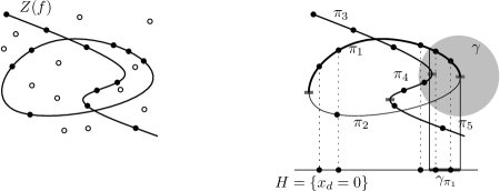
Figure 2: The zero set of the partitioning polynomial (left), and its decomposition into monotone patches that project to the hyperplane $H$ bijectively. Only the $1$-dimensional patches are labeled.

Following the terminology in [13, 26], we call a direction $v\in{\mathbb{S}}^{d-1}$ good for $f$ if, for every $a\in{\mathbb{R}}^{d}$, the polynomial $p(t)=f(a+vt)$ does not vanish identically; that is, any line in direction $v$ intersects $Z(f)$ at finitely many points. As argued in [26, pp. 304–305 and pp. 314–315], a random direction is good for $f$ with probability 1. By choosing a good direction and rotating the coordinate system, we assume that the $x_{d}$-direction, referred to as the vertical direction, is good for $f$.

In order to deal with $P^{*}$, we partition $Z(f)$ into finitely many pieces, called patches, in such a way that each of the patches is monotone in the vertical direction, meaning that every line parallel to the $x_{d}$-axis intersects it at most once. This is illustrated, in the somewhat trivial 2-dimensional setting, in Fig. 2 (right): there are five one-dimensional patches $\pi_{1},\ldots,\pi_{5}$, plus four 0-dimensional patches. Then we treat each patch $\pi$ separately: We project the point set $P^{*}\cap\pi$ orthogonally to the coordinate hyperplane $H:=\{x_{d}=0\}$, and we preprocess the projected set, denoted $P^{*}_{\pi}$, for range searching with suitable ranges. These ranges are projections of ranges of the form $\gamma\cap\pi$, where $\gamma\in\Gamma_{d,\Delta,s}$ is one of the original ranges. In Fig. 2  (right), the patch $\pi_{1}$ is drawn thick, a range $\gamma$ is depicted as a gray disk, and the projection $\gamma_{\pi_{1}}$ of $\gamma\cap\pi_{1}$ is shown as a thick segment in $H$.

The projected range $\gamma_{\pi}$ is typically more complicated than the original range $\gamma$ (it involves more polynomials of larger degrees), but, crucially, it is only $(d-1)$-dimensional, and $(d-1)$-dimensional queries can be processed somewhat more efficiently than $d$-dimensional ones, which makes the whole scheme work. We will discuss this in more detail in Section 7 below, but first we recall the notion of cylindrical algebraic decomposition (CAD, or also Collins decomposition), which is a tool that allows us to decompose $Z(f)$ into monotone patches, and also to compute the projected ranges $\gamma_{\pi}$.

Given a finite set $\mathcal{F}=\{f_{1},\ldots,f_{s}\}$ of $d$-variate polynomials, a cylindrical algebraic decomposition adapted to $\mathcal{F}$ is a way of decomposing ${\mathbb{R}}^{d}$ into a finite collection of relatively open cells, which have a simple shape (in a suitable sense), and which refine the arrangement $\mathcal{A}(\mathcal{F})$. We refer, e.g., to [5, Chap. 5.12] for the definition and construction of the “standard” CAD. Here we will use a simplified variant, which can be regarded as the “first stage” of the standard CAD, and which is captured by [5, Theorem 5.14, Algorithm 12.1]. We also refer to [26, Appendix A] for a concise treatment, which is perhaps more accessible at first encounter.

Let $\mathcal{F}$ be as above. To obtain the first-stage CAD for $f$, one constructs a suitable collection $\mathcal{E}=\mathcal{E}(\mathcal{F})$ of polynomials in the variables $x_{1},\ldots,x_{d-1}$ (denoted by ${\rm Elim}_{X_{k}}(\mathcal{F})$ in [5]). Roughly speaking, the zero sets of the polynomials in $\mathcal{E}$, viewed as subsets of the coordinate hyperplane $H$ (which is identified with ${\mathbb{R}}^{d-1}$), contain the projection onto $H$ of all intersections $Z(f_{i})\cap Z(f_{j})$, $1\leq i<j\leq s$, as well as the projection of the loci in $Z(f_{i})$ where $Z(f_{i})$ has a vertical tangent hyperplane, or a singularity of some kind. The actual construction of $\mathcal{E}$ is somewhat more complicated, and we refer to the aforementioned references for more details.

Figure 3: A schematic illustration of the first-stage cylindrical algebraic decomposition.

Having constructed $\mathcal{E}$, the first-stage CAD is obtained as the arrangement $\mathcal{A}(\mathcal{F}\cup\mathcal{E})$ in ${\mathbb{R}}^{d}$, where the polynomials in $\mathcal{E}$ are now considered as $d$-variate polynomials (in which the variable $x_{d}$ is not present). In geometric terms, we erect a “vertical wall” in ${\mathbb{R}}^{d}$ over each zero set within $H$ of a $(d-1)$-variate polynomial from $\mathcal{E}$, and the CAD is the arrangement of these vertical walls plus the zero sets of $f_{1},\ldots,f_{s}$. The first-stage CAD is illustrated in Fig. 3, for the same (single) polynomial as in Fig. 2 (left).

In our algorithm, we are interested in the cells of the CAD that are contained in some of the sero sets $Z(f_{i})$; these are going to be the monotone patches alluded to above. We note that using the first-stage CAD for the purpose of decomposing $Z(f)$ into monotone patches seems somewhat wasteful. For example, the number of patches in Fig. 2 is considerably smaller than the number of patches in the CAD in Fig. 3. But the CAD is simple and well known, and (as will follow from the analysis in Section 7) possible improvements in the number of patches (e.g. using the vertical-decomposition technique [27]) do not seem to influence our asymptotic bounds on the performance of the resulting range-searching data structure. The following lemma summarizes the properties of the first-stage CAD that we will need; we refer to [5, Theorem 5.14, Algorithm 12.1] for a proof.

Lemma 6.1 (Single-stage CAD).

Given a set $\mathcal{F}=\{f_{1},\ldots,f_{s}\}\subset{\mathbb{R}}[x_{1},\ldots,x_{d}]$ of polynomials, each of degree at most $D$, there is a set $\mathcal{E}=\mathcal{E}(\mathcal{F})$ of $O(s^{2}D^{3})$ polynomials in ${\mathbb{R}}[x_{1},\ldots,x_{d-1}]$, each of degree $O(D^{2})$, which can be computed in time $s^{2}D^{O(d)}$, such that the first-stage CAD defined by these polynomials, i.e., the arrangement $\mathcal{A}(\mathcal{F}\cup\mathcal{E})$ in ${\mathbb{R}}^{d}$, has the following properties:

1. (“Cylindrical” cells) For each cell $\sigma$ of $\mathcal{A}(\mathcal{F}\cup\mathcal{E})$, there exists a unique cell $\tau$ of the $(d-1)$-dimensional arrangement $\mathcal{A}(\mathcal{E})$ in $H$, such that one of the following possibilities occur:

   1. $\sigma=\{(x,\xi(x))\mid x\in\tau\}$, where $\xi\colon\tau\to{\mathbb{R}}$ is a continuous semialgebraic function (that is, $\sigma$ is the graph of $\xi$ over $\tau$).

   2. $\sigma=\{(x,t)\mid x\in\tau,t\in(\xi_{1}(x),\xi_{2}(x))\}$, where each $\xi_{i}$, $i=1,2$, is either a continuous semialgebraic real-valued function on $\tau$, or the constant function $\tau\to\{\infty\}$, or the constant function $\tau\to\{-\infty\}$, and $\xi_{1}(x)<\xi_{2}(x)$ for all $x\in\tau$ (that is, $\sigma$ is a portion of the “cylinder” $\tau\times{\mathbb{R}}$ between two consecutive graphs).

2. (Refinement property) If $\mathcal{F}^{\prime}\subseteq\mathcal{F}$, then $\mathcal{E}^{\prime}=\mathcal{E}(\mathcal{F}^{\prime})\subseteq\mathcal{E}$, and thus each cell of $\mathcal{A}(\mathcal{F}\cup\mathcal{E})$ is fully contained in some cell of $\mathcal{A}(\mathcal{F}^{\prime}\cup\mathcal{E}^{\prime})$.

Returning to the problem of decomposing the zero set of the partitioning polynomial $f$ into monotone patches, we construct the first-stage CAD for $\mathcal{F}=\{f\}$, and the patches are the cells of $\mathcal{A}(\mathcal{F}\cup\mathcal{E})$ contained in $Z(f)$. If the $x_{d}$-direction is good for $f$, then every cell of $\mathcal{A}(\mathcal{F}\cup\mathcal{E})$ lying in $Z(f)$ is of type (a), and so if any cell of type (b) lies in $Z(f)$, we choose another random direction and construct the first-stage CAD in that direction. Putting everything together and using Theorem 4.1 to bound the complexity of $\mathcal{A}(\mathcal{F}\cup\mathcal{E})$, we obtain the following lemma.

Lemma 6.2.

Let $f$ be a $d$-variate polynomial of degree $D$, and let us assume that the $x_{d}$-direction is good for $f$. Then $Z(f)$ can be decomposed, in $D^{O(d^{4})}$ time, into $D^{O(d)}$ monotone patches, and each patch can be represented semialgebraically by $D^{O(d^{4})}$ polynomials of degree $D^{O(d^{3})}$.

The first-stage CAD can also be used to compute the projection of the intersection of a range in $\Gamma_{d,\Delta,s}$ with a monotone patch of $f$.

Lemma 6.3.

Let $\Pi$ be the decomposition of the zero set of a $d$-variate polynomial $f$ of degree $D$ into monotone patches, as described in Lemma 6.2, and let $\gamma$ be a semialgebraic set in $\Gamma_{d,\Delta,s}$, with $\Delta\leq D$. For every patch $\pi\in\Pi$, the projection of $\gamma\cap\pi$ in the $x_{d}$-direction can be represented as a member of $\Gamma_{d-1,\Delta_{1},s_{1}}$, i.e., by a Boolean combination of at most $s_{1}$ polynomial inequalities in $(d-1)$ variables, each of degree at most $\Delta_{1}$, where $\Delta_{1}=D^{O(d^{3})}$ and $s_{1}=(Ds)^{O(d^{4})}$. The representation can be computed in $(Ds)^{O(d^{4})}$ time.

• The task of computing $\gamma_{\pi}$, the projection of $\gamma\cap\pi$, is similar to the operation (A2) discussed in Section 4. In more abstract terms, it can also be viewed as a quantifier elimination task: we can represent $\gamma\cap\pi$ by a quantifier-free formula $\Phi(x_{1},\ldots,x_{d})$ (a Boolean combination of polynomial inequalities); then $\gamma_{\pi}$ is represented by $\exists x_{d}\Phi(x_{1},\ldots,x_{d})$, and by eliminating $\exists x_{d}$ we obtain a quantifier-free formula describing $\gamma_{\pi}$. More concretely, we use a procedure based on the first-stage CAD (Lemma 6.1) and the arrangement construction (Theorem 4.1).

  By definition, $\gamma$ is a Boolean combination of inequalities of the form $g_{1}\geq 0,\ldots,g_{s}\geq 0$, where $g_{1},\ldots,g_{s}$ are $d$-variate polynomials, each of degree at most $\Delta\leq D$. We set $\tilde{\mathcal{F}}:=\{f,g_{1},\ldots,g_{s}\}$, we compute the set $\tilde{\mathcal{E}}=\mathcal{E}(\tilde{\mathcal{F}})$ of $(d-1)$-variate polynomials as in Lemma 6.1, and the first-stage CAD is then computed as the $d$-dimensional arrangement $\mathcal{A}(\tilde{\mathcal{F}}\cup\tilde{\mathcal{E}})$ according to Theorem 4.1. Since by Lemma 6.1(ii), $\mathcal{A}(\tilde{\mathcal{F}}\cup\tilde{\mathcal{E}})$ refines $\mathcal{A}(\{f\}\cup\mathcal{E}(\{f\}))$ (the first-stage CAD from the preprocessing phase), each patch $\pi\in\Pi$ is decomposed into subpatches. Since the sign of each $g_{i}$ is constant on each cell of $\mathcal{A}(\tilde{\mathcal{F}})$, and thus on each cell of $\mathcal{A}(\tilde{\mathcal{F}}\cup\tilde{\mathcal{E}})$, $\gamma\cap\pi$ is a disjoint union of subpatches. The projections of these subpatches into $H$ are cells of $\mathcal{A}(\tilde{\mathcal{E}})$, and thus we obtain, in time $(Ds)^{O(d^{4})}$, a representation of $\gamma_{\pi}$ as a member of $\Gamma_{d-1,\Delta_{1},s_{1}}$ by Theorem 4.1, where $\Delta_{1}=D^{O(d^{3})}$ and $s_{1}=(Ds)^{O(d^{4})}$. ∎

7 Large Fan-Out Partition Tree: Proof of Theorem 1.4

We now describe our second data structure for ${\Gamma}_{d,\Delta,s}$-range searching. Compared to the first data structure from Section 5, this one works on arbitrary point sets, without the $D_{0}$-general position assumption, or, alternatively, without the fuzzy boundary constraint on the output, and has slightly better performance bounds. The data structure is built recursively, and this time the recursion involves both $n$ and $d$.

7.1 The data structure

Let $P$ be a set of $n$ points in ${\mathbb{R}}^{d}$, and let $\Delta$ and $s$ be parameters (not assumed to be constant). The data structure for $\Gamma_{d,\Delta,s}$-range searching on $P$ is obtained by constructing a partition tree $\mathcal{T}$ on $P$ recursively, as above, except that now the fan-out of each node is larger (and non-constant), and each node also stores an auxiliary data structure for handling the respective exceptional part. We need to set two parameters: $n_{0}=n_{0}(d,\Delta,s)$ and $r=r(d,\Delta,s,n)$. Neither of them is a constant in general; in particular, $r$ is typically going to be a tiny power of $n$. The specific values of these parameters will be specified later, when we analyze the query time.

We also note that there is yet another parameter in Theorem 1.4, namely, the arbitrarily small constant $\varepsilon>0$ entering the preprocessing time bound. However, $\varepsilon$ enters the construction solely by the requirement that $r$ should be chosen smaller than $n^{\varepsilon/c}$, for a sufficiently large constant $c$. It will become apparent later in the analysis that $r\leq n^{\varepsilon/c}$ can be assumed, provided that some other parameters are taken sufficiently large; we will point this out at suitable moments.

When constructing the partition tree $\mathcal{T}$ on an $n$-point set $P$, we distinguish two cases. For $n\leq n_{0}$, $\mathcal{T}$ consists of a single leaf storing all points of $P$. For $n>n_{0}$, we construct an $r$-partitioning polynomial $f$ of degree $D=O(r^{1/d})$, the partition $\Omega$ of ${\mathbb{R}}^{d}$ induced by $f$, and the partition of $P$ into the exceptional part $P^{*}$ and regular parts $P_{1},\ldots,P_{t}$, where $t=O(r)$. Set $n^{*}=|P^{*}|$ and $n_{i}=|P_{i}|$, for $i=1,\ldots,t$. The root of $\mathcal{T}$ stores $f$, $\Omega$, and the total weight $w(P_{i})$ of each regular part $P_{i}$ of $P$, as before. Still in the same way as before, we recursively preprocess each regular part $P_{i}$ for $\Gamma_{d,\Delta,s}$-range searching (or stop if $|P_{i}|\leq n_{0}$), and attach the resulting data structure to the root as a respective subtree.

Handling the exceptional part.

A new feature of the second data structure is that we also preprocess the exceptional set $P^{*}$ into an auxiliary data structure, which is stored at the root. Here we recurse on the dimension, exploiting the fact that $P^{*}$ lies on the algebraic variety $Z(f)$ of dimension at most $d-1$.

We choose a random direction $v$ and rotate the coordinate system so that $v$ becomes the direction of the $x_{d}$-axis. We construct the first-stage CAD adapted to $\{f\}$, according to Lemma 6.1 and Theorem 4.1. We check whether all the patches are $x_{d}$-monotone, i.e., of type (a) in Lemma 6.1(i); if it is not the case, we discard the CAD and repeat the construction, with a different random direction. This yields a decomposition of $Z(f)$ into a set $\Pi$ of $D^{O(d)}$ monotone patches, and the running time is $D^{O(d^{4})}$ with high probability.

Next, we distribute the points of $P^{*}$ among the patches: for each patch $\pi\in\Pi$, let $P^{*}_{\pi}$ denote the projection of $P^{*}\cap\pi$ onto the coordinate hyperplane $H=\{x\in{\mathbb{R}}^{d}\,\mid\,x_{d}=0\}$. We preprocess each set $P^{*}_{\pi}$ for $\Gamma_{d-1,\Delta_{1},s_{1}}$-range searching. Here $s_{1}=(Ds)^{O(d^{4})}$ is the number of polynomials defining a range and $\Delta_{1}=D^{O(d^{3})}$ is their maximum degree; the constants hidden in the $O(\cdot)$ notation are the same as in Lemma 6.3. For simplicity, we treat all patches as being $(d-1)$-dimensional (although some may be of lower dimension); this does not influence the worst-case performance analysis.

The preprocessing of the sets $P^{*}_{\pi}$ is done recursively, using an $r_{1}$-partitioning polynomial in ${\mathbb{R}}^{d-1}$, for a suitable value of $r_{1}$. The exceptional set at each node of the resulting “$(d-1)$-dimensional” tree is handled in a similar manner, constructing an auxiliary data structure in $d-2$ dimensions, based on a first-stage CAD, and storing it at the corresponding node. The recursion on $d$ bottoms out at dimension $1$, where the structure is simply a standard binary search tree over the resulting set of points on the $x_{1}$-axis. We remark that the treatment of the top level of recursion on the dimension will be somewhat different from that of deeper levels, in terms of both the choice of parameters and the analysis; see below for details.

This completes the description of the data structure, except for the choice of $r$ and $n_{0}$, which will be provided later as we analyze the performance of the algorithm.

Answering a query.

Let us assume that, for a given $P$, the data structure for ${\Gamma}_{d,\Delta,s}$-range searching, as described above, has been constructed, and consider a query range $\gamma\in{\Gamma}_{d,\Delta,s}$. The query is answered in the same way as before, by visiting the nodes of the partition tree $\mathcal{T}$ in a top-down manner, except that, at each node that we visit, we also query with $\gamma$ the auxiliary data structure constructed on the exceptional set $P^{*}$ for that node.

Specifically, for each patch $\pi$ of the corresponding collection $\Pi$, we compute $w_{\pi}$, the weight of $P^{*}\cap(\gamma\cap\pi)$. If $\gamma\cap\pi=\emptyset$ then $w_{\pi}=0$, and if $\gamma\cap\pi=\pi$ then $w_{\pi}$ is the total weight of $P^{*}\cap\pi$. Otherwise, i.e., if $\gamma$ crosses $\pi$, then $w_{\pi}$ is the same as the weight of $P^{*}_{\pi}\cap\gamma_{\pi}$, where $\gamma_{\pi}$ is the $x_{d}$-projection of $\gamma\cap\pi$, because $\pi$ is $x_{d}$-monotone. By Lemma 6.3, $\gamma_{\pi}\in\Gamma_{d-1,\Delta_{1},s_{1}}$ and can be constructed in $(Ds)^{O(d^{4})}$ time. We can find the weight of $\gamma_{\pi}\cap P^{*}_{\pi}$ by querying the auxiliary data structure for $P^{*}_{\pi}$ with $\gamma_{\pi}$. We then add $w_{\pi}$ to the global count maintained by the query procedure. This completes the description of the query procedure.

7.2 Performance analysis

The analysis of the storage requirement and preprocessing time is straightforward, and will be provided later. We begin with the more intricate analysis of the query time. For now we assume that $n_{0}$ and $r$ have been fixed; the analysis will later specify their values.

Let $\mathsf{Q}_{d}(n,\Delta,s)$ denote the maximum overall query time for ${\Gamma}_{d,\Delta,s}$-range searching on a set of $n$ points in ${\mathbb{R}}^{d}$. For $n\leq n_{0}$ and $d\geq 1$, $\mathsf{Q}_{d}(n,\Delta,s)=O(n)$. For $d=1$ and $n>n_{0}$, $\mathsf{Q}_{1}(n,\Delta,s)=O(\Delta s\log n)$ because any range in $\Gamma_{1,\Delta,s}$ is the union of at most $\Delta s$ intervals. Finally, for $d>1$ and $n>n_{0}$, an analysis similar to the one in Section 5 gives the following recurrence for $\mathsf{Q}_{d}(n,\Delta,s)$:

$$\mathsf{Q}_{d}(n,\Delta,s)\leq C\Delta sr^{1-1/d}\mathsf{Q}_{d}(n/r,\Delta,s)+\sum_{\pi\in\Pi}\mathsf{Q}_{d-1}(n_{\pi},\Delta_{1},s_{1})+r^{c},$$ (1)

where $c=d^{O(1)}$, $C$ is a constant depending on $d$, $\sum_{\pi}n_{\pi}\leq n$, and both $|\Pi|$ and $\Delta_{1}s_{1}$ are bounded by $(Ds)^{a_{d}}$ with $D=O(r^{1/d})$ and $a_{d}=O(d^{4})$. (These are rather crude estimates, but we prefer simplicity.) The leading term of the recurrence relies on the crossing-number bound given in Lemma 4.3. In order to apply that lemma, we need that $r\geq\Delta^{d}$, which will be ensured by the choice of $r$ given below. The second term corresponds to querying the auxiliary data structures for the exceptional set $P^{*}$. The last term covers the time spent in computing the cells of the polynomial partition crossed by the query range $\gamma$ and for computing the projections $\gamma_{\pi}$ for every $\pi\in\Pi$; here we assume that the choice of $r$ will be such that $r\geq Ds$.

Ultimately, we want to derive that if $\Delta,s$ are constants, the recurrence (1) implies, with a suitable choice of $r$ and $n_{0}$ at each stage,

$$\mathsf{Q}_{d}(n,\Delta,s)\leq n^{1-1/d}\log^{B(d,\Delta,s)}n,$$ (2)

where $B(d,\Delta,s)$ is a constant depending on $d,\Delta$, and $s$.

However, as was already mentioned, even if $\Delta,s$ are constants initially, later in the recursion they are chosen as tiny powers of $n$, and this makes it hard to obtain a direct inductive proof of (2). Instead, we proceed in two stages. First, in Lemma 7.1 below we derive, without assuming $\Delta,s$ to be constants, a weaker bound for $\mathsf{Q}_{d}(n,\Delta,s)$, for which the induction is easier. Then we obtain the stronger bound (2) for constant values of $\Delta,s$ by using the weaker bound for the $(d-1)$-dimensional queries on the exceptional parts, i.e., for the second term in the recurrence (1).

A weaker bound for lower-dimensional queries.

Lemma 7.1.

For every $\nu>0$ there exists $A_{d,\nu}$ such that, with a suitable choice of $r$ and $n_{0}$,

$$\mathsf{Q}_{d}(n,\Delta,s)\leq(\Delta s)^{A_{d,\nu}}n^{1-1/d+\nu}$$ (3)

for all $d,n,\Delta,s$ (with $\Delta s\geq 2$, say).

Remarks.

(i) This lemma may look similar to our first result on $\Gamma_{d,\Delta,s}$-range searching, Theorem 1.2, but there are two key differences—the lemma works for arbitrary point sets, with no general position assumption, and $\Delta$ and $s$ are not assumed to be constants.

(ii) Since query time $O(n)$ is trivial to achieve, we may assume $\nu<1/d$, for otherwise, the bound (3) in the lemma exceeds $n$.

• The case $d=1$ is trivial because $Q_{1}(n,\Delta,s)\leq C\Delta s\log_{2}n$ clearly implies (3), assuming that $A_{d,\nu}\geq 1+\log_{2}C$ and that $n$ is sufficiently large so that $\log_{2}n\leq n^{\nu}$. We assume that (3) holds up to dimension $d-1$ (for all $\nu>0$, $\Delta$, $s$, and $n$), and we establish it for dimension $d$ by induction on $n$. We consider $A_{d,\nu}$ yet unspecified but sufficiently large; from the proof below one can obtain an explicit lower bound that $A_{d,\nu}$ should satisfy. We set

  $$n_{0}=n_{0}(d,\Delta,s,\nu):=(\Delta s)^{dA_{d,\nu}}\quad\mbox{and}\quad r=(2C\Delta s)^{1/\nu}.$$

  This value of $n_{0}$ is roughly the threshold where the bound (3) becomes smaller than $n$. Since we assume $\nu<1/d$, our choice of $r$ satisfies the assumptions $r\geq\Delta^{d}$ and $r\geq Ds$, as needed in (1).

  In the inductive step, for $n\leq n_{0}$,

  $$Q_{d}(n,\Delta,s)\leq n\leq n_{0}^{1/d}n^{1-1/d}=(\Delta s)^{A_{d,\nu}}n^{1-1/d}\leq(\Delta s)^{A_{d,\nu}}n^{1-1/d+\nu}.$$

  So we assume that $n>n_{0}$ and that the bound (3) holds for all $n^{\prime}<n$. Using the induction hypothesis, i.e., plugging (3) into the recurrence (1), we obtain

  $$\mathsf{Q}_{d}(n,\Delta,s) \leq C\Delta sr^{1-1/d}(\Delta s)^{A_{d,\nu}}(n/r)^{1-1/d+\nu}+|\Pi|(\Delta_{1}s_{1})^{A_{d-1,\nu}}n^{1-1/(d-1)+\nu}+r^{c}.$$ (4)

  By the choice of $r$, the first term of the right-hand side of (4) can be bounded by

  $$C\Delta sr^{-\nu}(\Delta s)^{A_{d,\nu}}n^{1-1/d+\nu}=\frac{1}{2}(\Delta s)^{A_{d,\nu}}n^{1-1/d+\nu},$$

  which is half of the bound we are aiming for.

  Next, we bound the second term. We use the estimates $\Delta_{1}s_{1}\leq(Ds)^{a_{d}}$, $|\Pi|\leq(Ds)^{a_{d}}$, and $Ds\leq r$. Then

  $$|\Pi|(\Delta_{1}s_{1})^{A_{d-1,\nu}}n^{1-1/(d-1)+\nu} \leq r^{a_{d}(A_{d-1,\nu}+1)}n^{1-1/(d-1)+\nu}$$ (5)

  $$\leq \frac{r^{a_{d}(A_{d-1,\nu}+1)}}{n^{1/d(d-1)}}\cdot n^{1-1/d+\nu}.$$

  We choose

  $$A_{d,\nu}=\frac{d-1}{\nu}a^{\prime}a_{d}(A_{d-1,\nu}+1),$$ (6)

  where $a^{\prime}=\log_{2}(4C)$; i.e., we choose $A_{d,\nu}=d^{\Theta(d)}/\nu^{d}$. Since $n\geq n_{0}=(\Delta s)^{dA_{d,\nu}}$ and $r=(2C\Delta s)^{1/\nu}$, the fraction in (5) can be bounded by

  $$\frac{r^{a_{d}(A_{d-1,\nu}+1)}}{n^{1/d(d-1)}} \leq\frac{(2C\Delta s)^{A_{d,\nu}/a^{\prime}(d-1)}}{(\Delta s)^{A_{d,\nu}/(d-1)}}\leq\left(\frac{2C}{(\Delta s)^{a^{\prime}-1}}\right)^{A_{d,\nu}/a^{\prime}(d-1)}\leq 1$$

  because $\Delta s\geq 2$.

  Finally, recall that $c=d^{O(1)}$, so our choice of $A_{d,\nu}$ (again, choosing $a^{\prime}$ sufficiently large) ensures that $r^{c}<n^{1-1/d}$. Hence, the right hand side in (4) is bounded by

  $$\tfrac{1}{2}(\Delta s)^{A_{d,\nu}}n^{1-1/d+\nu}+2n^{1-1/d+\nu}\leq(\Delta s)^{A_{d,\nu}}n^{1-1/d+\nu},$$

  as desired. This establishes the induction step and thereby completes the proof of the lemma. ∎

The improved bound for the query time.

Now we want to obtain the improved bound (2), i.e., $\mathsf{Q}_{d}(n,\Delta,s)\leq n^{1-1/d}\log^{B}n$, with $B=B(d,\Delta,s)$, assuming that $\Delta,s$ are constants and $n>2$. To this end, in the top-level ($d$-dimensional) partition tree, we set $r:=n^{\delta}$, where $\delta>0$ is a suitable small constant to be specified later. Then we use the result of Lemma 7.1 with $\nu:=\frac{1}{2d(d-1)}$ for processing the $(d-1)$-dimensional queries on the sets $P^{*}_{\pi}$. Thus, in the forthcoming proof, we do induction only on $n$, while $d$ is fixed throughout.

We choose $n_{0}=n_{0}(d,\Delta,s)$ sufficiently large (we will specify this more precisely later on), and we assume that $n>n_{0}$ and that the desired bound (2) holds for all $n^{\prime}<n$. In the inductive step we estimate, using the recurrence (1), the induction hypothesis, and the bound in (3),

$$\mathsf{Q}_{d}(n,\Delta,s)\leq C\Delta sr^{1-1/d}(n/r)^{1-1/d}\log^{B}(n/r)+|\Pi|(\Delta_{1}s_{1})^{A_{d-1,\nu}}n^{1-1/(d-1)+\nu}+r^{c}.$$

The first term simplifies to $(1-\delta)^{B}C\Delta sn^{1-1/d}\log^{B}n$. Thus, if we choose $B$ depending on $\delta$ (which is a small positive constant still to be determined) so that $(1-\delta)^{B}C\Delta s\leq\frac{1}{2}$, then the first term will be at most half of the target value $n^{1-1/d}\log^{B}n$. Thus, it suffices to set $\delta$ so that the remaining two terms are negligible compared to this value.

For the $r^{c}$ term, any $\delta\leq 1/2c$ will do. The second term can be bounded, as in the proof of Lemma 7.1, by

$$r^{a_{d}(A_{d-1,\nu}+1)}n^{1-1/(d-1)+\nu}=\frac{r^{\nu A_{d,\nu}/(a^{\prime}(d-1))}}{n^{\nu}}\cdot n^{1-1/d}.$$

Thus, with $\delta\leq a^{\prime}(d-1)/A_{d,\nu}$, the term is at most $n^{1-1/d}$. Again, this establishes the induction step and concludes the proof of the final bound for the query time. We remark that our choice of $\delta$ requires us to choose

$$B\approx\frac{1}{\delta}\ln(2C\Delta s)\approx\ln(2C\Delta s)\cdot d^{\Theta(d)},$$

making its dependence on $d$ super-exponential.

Analysis of storage and preprocessing.

Let $\mathsf{S}_{d}(n,\Delta,s)$ denote the size of the data structure on $n$ points in ${\mathbb{R}}^{d}$ for ${\Gamma}_{d,\Delta,s}$-range searching, with the settings of $r$ and $n_{0}$ as described above. For $n\leq n_{0}=n_{0}(d,\Delta,s)$ we have $\mathsf{S}_{d}(n,\Delta,s)=O(n)$. For larger values of $n$, the space occupied by the root of the partition tree, not counting the auxiliary data structure for the exceptional part $P^{*}$, is bounded by $r^{c}$, where $c=d^{O(1)}$. Furthermore, since $\mathsf{S}_{d}(n,\Delta,s)$ is at least linear in $n$, the total size of the auxiliary data structure constructed on $P^{*}$ is $\sum_{\pi\in\Pi}\mathsf{S}_{d-1}(n_{\pi},\Delta_{1},s_{1})\leq\mathsf{S}_{d-1}(n^{*},\Delta_{1},s_{1})$, where $n^{*}=|P^{*}|$. We thus obtain the following recurrence for $\mathsf{S}_{d}(n,\Delta,s)$:

$$\mathsf{S}_{d}(n,\Delta,s)\leq\displaystyle\sum_{i=1}^{t}\mathsf{S}_{d}(n_{i},\Delta,s)+\mathsf{S}_{d-1}(n^{*},\Delta_{1},s_{1})+O(r^{c})$$

for $n>n_{0}=n_{0}(d,\Delta,s)$, and $\mathsf{S}_{d}(n,\Delta,s)=O(n)$ for $n\leq n_{0}$. Using $n_{i}\leq n/r$, $n^{*}+\sum_{i}n_{i}\leq n$, and $r^{c}=o(n)$, for both types of choices of $r$, the recurrence easily leads to

$$\mathsf{S}_{d}(n,\Delta,s)=O(n),$$

where the constant of proportionality depends on $d$.

It remains to estimate the preprocessing time; here, finally, the parameter $\varepsilon>0$ in Theorem 1.4 comes into play. Let $\delta^{*}$ be a constant such that $r\leq n^{\delta^{*}}$ (at all stages of the algorithm). As was remarked in the preceding analysis of the query time, we can make $\delta^{*}$ arbitrarily small, by adjusting various constants (and, generally speaking and as already remarked above, the smaller $\delta^{*}$, the worse constant $B(d,\Delta,s)$ we obtain in the query time bound).

Let $\mathsf{T}_{d}(n,\Delta,s,\delta^{*})$ denote the maximum preprocessing time of our data structure for $\Gamma_{d,\Delta,s}$-range searching on $n$ points, with $\delta^{*}>0$ a constant as above. Using the operation (A1) of Section 4, we spend $O(nr^{c})$ time to compute $\Omega(f)$ and the partition of $P$ into the exceptional part and the regular parts, and we spend additional $O(nr^{c})$ time to compute $\Pi$ and $P^{*}_{\pi}$ for every $\pi\in\Pi$, where $c=d^{O(1)}$. The total time spent in constructing the secondary data structures for all patches of $\Pi$ is bounded by $\mathsf{T}_{d-1}(n^{*},\Delta_{1},s_{1},\delta^{*})$. Hence, we obtain the recurrence

$$\mathsf{T}_{d}(n,\Delta,s,\delta^{*})\leq\displaystyle\sum_{i=1}^{t}\mathsf{T}_{d}(n_{i},\Delta,s,\delta^{*})+\mathsf{T}_{d-1}(n^{*},\Delta_{1},s_{1},\delta^{*})+O(nr^{c})$$

for $n>n_{0}$, and $\mathsf{T}_{d}(n,\Delta,s,\delta^{*})=O(n)$ for $n\leq n_{0}$. Using the properties $n_{i}\leq n/r$ and $n^{*}+\sum_{i}n_{i}\leq n$, a straightforward calculation shows that

$$\mathsf{T}_{d}(n,\Delta,s,\delta^{*})=O(n^{1+c\delta^{*}}),$$

where the constant of proportionality depends on $d$. Hence, by choosing $\delta^{*}=\varepsilon/c$, the preprocessing time is $O(n^{1+\varepsilon})$. This concludes the proof of Theorem 1.4.

8 Open Problems

We conclude this paper by mentioning a few open problems.

(i) A very interesting and challenging problem is, in our opinion, the fast-query case of range searching with constant-complexity semialgebraic sets, where the goal is to answer a query in $O(\log n)$ time using roughly $n^{d}$ space. There are actually two, apparently distinct, issues. The standard approach to fast-query searching is to parameterize the ranges in $\Gamma$ by points in a space of a suitable dimension, say $t$; then the $n$ points of $P$ correspond to $n$ algebraic surfaces in this $t$-dimensional “parameter space”, and a query is answered by locating the point corresponding to the query range in the arrangement of these surfaces.

First, the arrangement has $O(n^{t})$ combinatorial complexity, and one would expect to be able to locate points in it in polylogarithmic time with storage about $n^{t}$. However, such a method is known only up to dimension $t=4$, and in higher dimension, one again gets stuck at the arrangement decomposition problem, which was the bottleneck in the previously known solution of [2] for the low-storage variant, as was mentioned in the introduction. It would be nice to use polynomial partitions to obtain a better point location data structure for such arrangements, but unfortunately, so far all of our attempts in this direction have failed.

The second issue is, whether the point location approach just sketched is actually optimal. This question is exhibited nicely already in the simple instance of range searching with disks in the plane. The best known solution that guarantees logarithmic query time uses point location in ${\mathbb{R}}^{3}$ and requires storage roughly $n^{3}$, but it is conceivable that roughly quadratic storage might suffice.

(ii) Our range-searching data structure for arbitrary point sets—the one with large fan-out—is so complex and has a rather high exponent in the polylogarithmic factor, because we have difficulty with handling highly degenerate point sets, where many points lie on low-degree algebraic surfaces. This issue appears even more strongly in combinatorial applications, and in that setting it has been dealt with only in rather specific cases (e.g., in dimension 3); see [15, 29, 34] for initial studies. It would be nice to find a construction of suitable “multilevel polynomial partitions” that would cater to such highly degenerate input sets, as touched upon in [15, 34].

(iii) Another open problem, related to the construction of polynomial partitions, is the fast evaluation of a multivariate polynomial at many points, as briefly discussed at the end of Section 3.

Acknowledgments.

We thank the anonymous referees for their useful comments on the paper.

References

- [1] P. K. Agarwal and J. Erickson, Geometric range searching and its relatives, in: Advances in Discrete and Computational Geometry (B. Chazelle, J. E. Goodman and R. Pollack, eds.), AMS Press, Providence, RI, 1998, pp. 1–56.
- [2] P. K. Agarwal and J. Matoušek, On range searching with semialgebraic sets, Discrete Comput. Geom. 11 (1994), 393–418.
- [3] S. Barone and S. Basu, Refined bounds on the number of connected components of sign conditions on a variety, Discrete Comput. Geom. 47 (2012), 577–597.
- [4] S. Basu, R. Pollack, and M.-F. Roy, On the number of cells defined by a family of polynomials on a variety, Mathematika 43 (1996), 120–126.
- [5] S. Basu, R. Pollack, and M.-F. Roy, Algorithms in Real Algebraic Geometry, Algorithms and Computation in Mathematics 10, Springer-Verlag, Berlin, 2003.
- [6] T. M. Chan, Optimal partition trees, Discrete Comput. Geom. 47 (2012), 661–690.
- [7] B. Chazelle, Lower bounds on the complexity of polytope range searching, J. Amer. Math. Soc. 2 (1989), 637–666.
- [8] B. Chazelle, H. Edelsbrunner, L. J. Guibas, and M. Sharir, A singly exponential stratification scheme for real semi-algebraic varieties and its applications, Theoret. Comput. Sci., 84 (1991), 77–105. Also in Proc. 16th Int. Colloq. on Automata, Languages and Programming (1989), pp. 179–193.
- [9] D. Cox, J. Little and D. O’Shea, Ideals, Varieties, and Algorithms: An Introduction to Computational Algebraic Geometry and Commutative Algebra, 2nd edition, Springer Verlag, Heidelberg, 1997.
- [10] Gy. Elekes, H. Kaplan and M. Sharir, On lines, joints, and incidences in three dimensions, J. Combinat. Theory, Ser. A 118 (2011), 962–977.
- [11] L. Guth and N. H. Katz, Algebraic methods in discrete analogs of the Kakeya problem, Advances Math. 225 (2010), 2828–2839.
- [12] L. Guth and N. H. Katz, On the Erdős distinct distances problem in the plane, in arXiv:1011.4105.
- [13] H. Hironaka, Triangulations of algebraic sets, in Proceedings of Symposia Pure Math (Robin Hartshorne, ed.), Vol. 29, Amer. Math. Soc., Providence, R.I., 1975, 165-185.
- [14] H. Kaplan, J. Matoušek and M. Sharir, Simple proofs of classical theorems in discrete geometry via the Guth–Katz polynomial partitioning technique, Discrete Comput. Geom. 48 (2012), 499–517.
- [15] H. Kaplan, J. Matoušek, Z. Safernová and M. Sharir, Unit distances in three dimensions, Combinat. Probab. Comput. 21 (2012), 597–610.
- [16] K. Kedlaya and Ch. Umans, Fast modular composition in any characteristic, Proc. 49th Annu. IEEE Sympos. Foundat. Comput. Sci. (2008), 146–155.
- [17] Ch. Knauer, H. R. Tiwari and D. Werner, On the computational complexity of Ham-Sandwich cuts, Helly sets, and related problems, Proc. 28th Annu. Sympos. Theoret. Aspects Comput. Sci. (2011), 649–660.
- [18] V. Koltun, Almost tight upper bounds for vertical decompositions in four dimensions, J. ACM 51(5) (2004), 699–730.
- [19] K. G. Larsen, On range searching in the group model and combinatorial discrepancy, Proc. 52nd Annu. IEEE Sympos. Found. Comp. Sci. (2011), 542–549.
- [20] C.-Y. Lo, J. Matoušek and W. Steiger, Ham-sandwich cuts in , Proc. 24th Annu. ACM Sympos. Theory Comput. Sci. (1992), 539–545.
- [21] J. Matoušek, Efficient partition trees, Discrete Comput. Geom. 8 (1992), 315–334.
- [22] J. Matoušek, Range searching with efficient hierarchical cuttings, Discrete Comput. Geom. 10 (1993), 157–182.
- [23] J. Matoušek, Geometric range searching, ACM Comput. Surv. 26(4) (1994), 421–461.
- [24] J. Matoušek, Using the Borsuk-Ulam Theorem, Lectures on Topological Methods in Combinatorics and Geometry Series, Springer Verlag, Heidelberg, 2003.
- [25] M. Nüsken and M. Ziegler, Fast multipoint evaluation of bivariate polynomials, Proc. 12th Annu. European Sympos. Algorithms (2004), 544–555.
- [26] J. T. Schwartz and M. Sharir, On the Piano Movers’ problem: II. General techniques for computing topological properties of real algebraic manifolds, Advances Appl. Math. 4 (1983), 298–351.
- [27] M. Sharir and P. K. Agarwal, Davenport Schinzel Sequences and Their Geometric Applications, Cambridge University Press, New York, 1995.
- [28] M. Sharir and H. Shaul, Semi-algebraic range reporting and emptiness searching with applications, SIAM J. Comput. 40 (2011), 1045–1074.
- [29] J. Solymosi and T. Tao, An incidence theorem in higher dimensions, Discrete Comput. Geom. 48 (2012), 255–280.
- [30] A. H. Stone and J. W. Tukey, Generalized sandwich theorems, Duke Math. J. 9 (1942), 356–359.
- [31] H. E. Warren, Lower bound for approximation by nonlinear manifolds, Trans. Amer. Math. Soc. 133 (1968), 167–178.
- [32] A. C. Yao and F. F. Yao, A general approach to -dimensional geometric queries, Proc. 17th Annu. ACM Sympos. Theory Comput., 163–168.
- [33] C. K. Yap, A geometric consistency theorem for a symbolic perturbation scheme, J. Comput. Syst. Sci. 40 (1990), 2–18.
- [34] J. Zahl, An improved bound on the number of point-surface incidences in three dimensions, in arXiv:1104.4987.