Higgs algebraic symmetry of screened system in a spherical geometry

Abstract

The orbits and the dynamical symmetries for the screened Coulomb potentials and isotropic harmonic oscillators have been studied by Wu and Zeng [Z. B. Wu and J. Y. Zeng, Phys. Rev. A 62,032509 (2000)]. We find the similar properties in the responding systems in a spherical space, whose dynamical symmetries are described by Higgs Algebra. There exists a conserved aphelion and perihelion vector, which, together with angular momentum, constitute the generators of the geometrical symmetry group at the aphelia and perihelia points $(\dot{r}=0)$.

1 Introduction

The classic Bertrand’s theorem says that there are two central fields only for which all bounded orbits are closed, namely, the Kepler’s problem (also known as the inverse square law) and the isotropic harmonic oscillator [1, 2, 3]. The both fields give rise to elliptical orbits, with the difference that in the first case the force is directed towards one of the foci and in the second case the force is directed to the geometrical center of the ellipse. Besides the energy and angular momentum, these elliptical orbits are guaranteed by an additional conserved quantity: the Runge-Lenz vector for Kepler’s problem [4, 5, 6, 7] and a quadrupole tensor for the isotropic harmonic oscillator [8, 9], which imply higher dynamical symmetries than the geometric symmetries [10, 11, 12]. In this paper, we pay attention to the two-dimensional cases, in which the angular momentum $\textbf{L}=L_{z}\textbf{k}$, the Runge-Lenz vector has two components

$$R_{x} = \frac{1}{2}(p_{y}L_{z}+L_{z}p_{y})-\frac{x}{r},$$ (1)

$$R_{y} = -\frac{1}{2}(p_{x}L_{z}+L_{z}p_{x})-\frac{y}{r},$$

and the components of the conserved tensor in oscillator are

$$Q_{xy}=xy+p_{x}p_{y},$$ (2)

$$Q_{1}=\frac{1}{2}[(x^{2}-y^{2})+(p_{x}^{2}-p_{y}^{2})].$$

Taking the classical orbit as his start point, Higgs [13] generalized the hydrogen atom and harmonic oscillator in the spherical space preserving the dynamical symmetry. He established a gnomonic projective coordinate system in which the orbit of the motion on a sphere can be described as

$$\frac{1}{2}L_{z}^{2}[r^{-4}(\frac{dr}{d\theta})^{2}+r^{-2}]+V(r)=E-\frac{1}{2}\lambda L_{z}^{2},$$ (3)

where the angular momentum $L_{z}=x_{1}p_{2}-x_{2}p_{1}$ is an invariant quantity with the radial symmetric potential $V(r)$. The curvature appears only in the right combination $E-\frac{1}{2}\lambda L_{z}^{2}$ of Eq. (3), and, therefore, the projected orbits are the same, for a given $V(r)$, as in Euclidean geometry.

To give a more clear description of Higgs’ result, we shall review the coordinate systems adopt in [13].

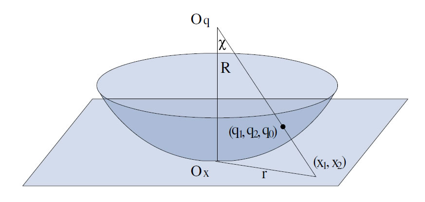
Figure 1: The gnomonic projection, which is the projection onto the tangent plane from the center of the sphere in the embedding space, and the coordinate systems

Consider the sphere embed in a three-dimensional Euclidean space, see Fig. 1. Then, each pair of independent variables $(q_{1},q_{2})$ of the three-dimensional Cartesian coordinates $(q_{1},q_{2},q_{0})$, with the origin $O_{q}$ in the figure, is obtained simply by imposing the constraint

$$q_{0}^{1}+q_{1}^{2}+q_{2}^{2}=\frac{1}{\lambda},$$ (4)

where $\lambda=\frac{1}{R^{2}}$ is the curvature of the sphere, in which R is the radius. The points on the sphere can also be described by the spherical coordinates $(R,\chi,\theta)$ which is defined by $(q_{1},q_{2},q_{0})=(R\sin\chi\cos\theta,R\sin\chi\sin\theta,R\cos\chi)$. On the other hand, the points can be expressed in terms of polar coordinates $(r,\theta)$. In the two-dimensional gnomonic projection, which is the projection onto the tangent plane from the center of the sphere in the embedding space, the Cartesian coordinates of this projection, denoted $(x_{1},x_{2})$, are given by

$$q_{1}=\frac{x_{1}}{\sqrt{1+\lambda r^{2}}},\ \ \ \ \ \ \ \ \ q_{2}=\frac{x_{2}}{\sqrt{1+\lambda r^{2}}},$$ (5)

where $r^{2}=x_{1}^{2}+x_{2}^{2}$ and the point of tangency $O_{x}$ in the figure is the origin. Then, the polar coordinates $(r,\theta)$ of the projection are determined by the relations $r=R\tan\chi$ and $(x_{1},x_{2})=(r\cos\theta,r\sin\theta)$.

Higgs demonstrated that in the gnomonic projection, the Hamiltonian in a spherical geometry, with the same classical orbits corresponding in a plane, can be written as

$$H=\frac{\pi^{2}}{2}+\frac{1}{2}\lambda L_{z}^{2}+V(r),$$ (6)

where $\vec{\pi}=\vec{p}+\frac{\lambda}{2}\left[\vec{x}(\vec{x}\cdot\vec{p})+(\vec{p}\cdot\vec{x})\vec{x}\right]$ is the conserved vector in free particle motion on the sphere. He gave the conserved quantities which commute with the Hamiltonian for the Coulomb potential and the isotropic oscillator. According to the Bertrand’s Theorem, the orbits are closed only if the potential takes the Coulomb or isotropic oscillator form, i.e. $V(r)=-\frac{1}{r}$ or $V(r)=\frac{1}{2}r^{2}$. The systems described by Eq. (6) with the two mentioned potentials are defined as the Kepler problem and isotropic oscillator in a spherical geometry in [13]. The algebraic relations of their conserved quantities reveal the dynamical symmetries of the two systems are described by the symmetry groups $SO(3)$ and $SU(2)$ respectively. This algebraic structure is called Higgs Algebra, and has received attention from a variety of literatures [14, 15, 16, 17, 18, 19, 20].

The Bertrand’s theorem has been extended in different directions [21, 22, 23, 24]. In the original theorem, the form of the central potential is assumed to be a power-law function of $r$ [2]. However, Wu and Zeng [21] believed that, if the restriction of a power-law form of the central potential is relaxed, Bertrand’s theorem may be extended. They showed that when the Coulomb potential or isotropic harmonic oscillator is screened [see Eq. (9) and Eq. (18)], the elliptic orbits are broken, but there still exist an infinite number of closed orbits. The broken orbit gives promise of that, the dynamical symmetry $SO(3)$ for hydrogen atom or $SU(2)$ for isotropic harmonic oscillator is broken, but the revival of closeness of some classical orbits may be an indication of the recurrence of the dynamical symmetry.

For the screened two-dimensional Coulomb potential, Wu and Zeng [21] noticed that the usual Runge-Lenz vector in Eq. (1) no longer remains conserved. While, they found that the extended Runge-Lenz vector with components given bellow

$$R^{\prime}_{x} = \frac{1}{2}(p_{y}L_{z}+L_{z}p_{y})-\left(1+\frac{2k}{r}\right)\frac{x}{r},$$ (7)

$$R^{\prime}_{y} = -\frac{1}{2}(p_{x}L_{z}+L_{z}p_{x})-\left(1+\frac{2k}{r}\right)\frac{y}{r},$$

are conserved at the aphelion (perihelion) points ($\dot{r}=0$). In other words, besides $\left[L_{z},H\right]=0$, it holds that $\left[R^{\prime}_{x},H\right]=0$ and$\left[R^{\prime}_{y},H\right]=0$ at the aphelion and perihelion points. Moreover, they satisfy the commutation relations

$$\left[L_{z},R^{\prime}_{x}\right] = iR^{\prime}_{y},$$ (8)

$$\left[L_{z},R^{\prime}_{y}\right] = -iR^{\prime}_{x},$$

$$\left[R^{\prime}_{x},R^{\prime}_{y}\right] = -2iHL_{z},$$

which imply that ($L_{z},R^{\prime}_{x},R^{\prime}_{y}$) constitute an $SO(3)$ algebra in Hilbert space spanned by degenerate states belonging to a given energy eigenvalue $E_{n}=-\frac{1}{2n^{2}}$. Here, $n=n_{r}+|m^{\prime}|+\frac{1}{2}$, where $n_{r}=0,1,2,\ldots$ and $m^{\prime}=\sqrt{m^{2}-2k}$ with $m=-n_{r},-n_{r}+1,\ldots,n_{r}$ is the eigenvalue of the conserved angular momentum $L_{z}$. The authors of [21] believed, in general, that the dynamical symmetry $SO(3)$ of a two-dimensional hydrogen atom is broken, and the $SO(3)$ symmetry may be restored at the aphelion and perihelion points of the classical orbits. Similar results have been obtained in the screened two-dimensional isotropic oscillator.

Since the construction of the systems in the sphere given by Higgs [13] is based on the orbits of classical motion, which is also the starting point in the work of Wu and Zeng [21], we speculate that similar results of the screened potentials in [21] can be found in Higgs’ sphere systems [13]. As the first attempt, we focus on two-dimensional spherical geometry. In Sec. 2, we will show the dynamical symmetry of screened Coulomb potential to a spherical geometry. Besides that, we give the eigenenergy and eigenstates of this system. A similar process for the screened isotropic harmonic oscillator will be presented in Sec. 3. A summary is made in the last section.

2 Screened Coulomb potential

Based on the results in [21], the classical orbit equation in the spherical system described by the Hamiltonian (6) with the screened Coulomb potential

$$V(r)=-\frac{1}{r}-\frac{k}{r^{2}}\ \ \ \ \ \ (0<k\ll 1),$$ (9)

can be obtained by using the relation in Eq. (3) as

$$\frac{1}{r}=\frac{1}{L_{z}^{2}\alpha^{2}}\left[1+\sqrt{1+2(E-\frac{1}{2}\lambda L_{z}^{2})L_{z}^{2}\alpha^{2}}\cos{(\alpha(\theta-\theta_{0}))}\right],$$ (10)

where $E<0$ and $\alpha=\sqrt{1-2k/L_{z}^{2}}<1$. When $\lambda\rightarrow 0$, the equation reduces to the screened Coulomb potential on a plane.

It should be noted that the orbit is not closed in general. However, for rational values of $\alpha$ (that is, for suitable angular momenta $L_{z}=\sqrt{2k/(1-\alpha^{2})}$), there still exist an infinite number of closed orbits whose geometry depends only on the angular momentum.

In the construction of Higgs, he replaced $\vec{p}$ in the original Runge-Lenz vector by $\vec{\pi}$, which is conserved in free motion in a spherical geometry, and obtained the Runge-Lenz vector in this space

$$R^{\prime}_{x}=\frac{1}{2}\left(\pi_{y}L_{z}+L_{z}\pi_{y}\right)-\left(1+\frac{2k}{r}\right)\frac{x}{r},$$ (11)

$$R^{\prime}_{y}=-\frac{1}{2}\left(\pi_{x}L_{z}+L_{z}\pi_{x}\right)-\left(1+\frac{2k}{r}\right)\frac{y}{r}.$$

By a direct calculation, we find that they are still conserved at the aphelion (perihelion) points ($\dot{r}=0$), i.e.,

$$\left[R^{\prime}_{x},H\right]=0,\ \ \ \ \ \ \left[R^{\prime}_{y},H\right]=0.$$ (12)

It can be shown that

$$\left[R^{\prime}_{x},L_{z}\right] = -iR^{\prime}_{y},$$ (13)

$$\left[R^{\prime}_{y},L_{z}\right] = iR^{\prime}_{x},$$

$$\left[R^{\prime}_{x},R^{\prime}_{y}\right] = i\left(-2H+2\lambda L_{z}^{2}+\frac{1}{4}\lambda-2k\lambda\right)L_{z}.$$

These equations imply that ($L_{z},R^{\prime}_{x},R^{\prime}_{y}$) constitute an polynomial Higgs algebra $SO(3)$ in Hilbert space spanned by degenerate states with a given energy eigenvalue $E_{n}$. But the identities in (12) hold only at the aphelion and the perihelion points. Therefore, in general, though the $SO(3)$ dynamical symmetry of two-dimensional spherical hydrogen atom is broken, it may be restored at the aphelion and perihelion points of the classical orbits. Because of angular momentum conservation, the classical orbits are still closed for rational values of $\alpha$.

For the purposes of getting the eigenvalues and the eigenstates simply, we adopt the polar coordinates $(r,\theta)$. The Hamiltonian of Higgs’ systems in a spherical geometry is

$$H=-\frac{1}{2}\left[3\lambda+\frac{15}{4}\lambda^{2}r^{2}+\frac{(1+\lambda r^{2})(1+5\lambda r^{2})}{r}\frac{\partial}{\partial r}+(1+\lambda r^{2})^{2}\frac{\partial^{2}}{\partial r^{2}}+\frac{1}{r^{2}}\frac{\partial^{2}}{\partial\theta^{2}}+\lambda\frac{\partial^{2}}{\partial\theta^{2}}\right]+V.$$ (14)

For a radial potential $V=V(r)$, the eigenfunction of energy can be written as

$$\Psi(r,\theta)=e^{im\theta}\psi(r),$$ (15)

with $m=0,\pm 1,\pm 2,...$ is the eigenvalue of the conserved angular momentum $L_{z}$. The Schrödinger equation $H\Psi(r,\theta)=E\Psi(r,\theta)$ reduces to the radial equation

$$H_{1}\psi(r)=E\psi(r).$$ (16)

Here, the Hamiltonian $H_{1}$ can be written as

$$H_{1}=-\frac{1}{2}\left[(1+\lambda r^{2})^{2}\frac{d^{2}}{dr^{2}}+\frac{(1+\lambda r^{2})(1+5\lambda r^{2})}{r}\frac{d}{dr}-\frac{1+\lambda r^{2}}{r^{2}}m^{\prime 2}+3\lambda+\frac{15}{4}\lambda^{2}r^{2}\right]+\frac{1}{r}+\lambda k,$$

where $m^{\prime}=\sqrt{m^{2}-2k}$, and $\lambda k$ is a real number independent of $r$. From the above equation, one could find that the eigenstates and the eigenvalues can be obtained by substituting $m$ with $m^{\prime}$ in the Coulomb potential system in the spherical geometry [13]. The eigenenergy is

$$E_{N,m}=\frac{1}{2}\lambda(m^{\prime}+N)(m^{\prime}+N+1)-\frac{1}{2}(m^{\prime}+N+\frac{1}{2})^{-2}+\lambda k,$$ (17)

where $N$ is a non-negative integer. But $\Delta m=\pm 1$ does not imply $\Delta m^{\prime}=\pm 1$, the degeneracy of energy splits. And the eigenstates $\Psi(r,\theta)=e^{im\theta}\psi(r)$, where $\psi(r)$ is the same as that in [13], except that $m^{\prime}$ takes the place of $m$. The above result (17) reduces to Higgs’ Coulomb potential described in [13] as $k\rightarrow 0$, and to the screened Coulomb potential described in [21] as $\lambda\rightarrow 0$.

3 Screened isotropic harmonic oscillator

In this section, we shall discuss the screened spherical isotropic harmonic oscillator described by the Hamiltonian (6) with the potential [23]

$$V(r)=\frac{1}{2}r^{2}-\frac{k}{r^{2}}.$$ (18)

Similarly, based on the results in [21] and together with equation (3), the orbit equation can be expressed as

$$\frac{1}{r^{2}}=\frac{1}{L_{z}^{2}\alpha^{2}}\left[E-\frac{1}{2}\lambda L_{z}^{2}+\sqrt{(E-\frac{1}{2}\lambda L_{z}^{2})^{2}-L_{z}^{2}\alpha^{2}}\cos{(2\alpha(\theta-\theta_{0}))}\right],$$ (19)

where $\alpha=\sqrt{1-2k/L_{z}^{2}}<1$. As $\lambda$ tends to 0, the equation reduces to the screened Coulomb potential on a plane. In this situation, the orbit is not closed in general. But, for rational values of $\alpha$, there still exist an infinite number of closed orbits.

For the isotropic harmonic oscillator in a spherical geometry, there exist the conserved quantities $L_{z},Q_{xy}=xy+\frac{1}{2}(\pi_{x}\pi_{y}+\pi_{y}\pi_{x}),$ and $Q_{1}=\frac{1}{2}[(x^{2}-y^{2})+(\pi_{x}^{2}-\pi_{y}^{2})]$ [13]. Combining the result in [21], we introduce the quantities

$$Q_{xy}^{\prime} = (1+\frac{2k}{r^{4}})xy+\frac{1}{2}(\pi_{x}\pi_{y}+\pi_{y}\pi_{x}),$$ (20)

$$Q_{1}^{\prime} = \frac{1}{2}\left[(1+\frac{2k}{r^{4}})(x^{2}-y^{2})+(\pi_{x}^{2}-\pi_{y}^{2})\right].$$

It can be shown that $[Q_{xy}^{\prime},H]=0$ and $[Q_{1}^{\prime},H]=0$ hold at the aphelion (perihelion) points of classical orbits $(\dot{r}=0)$. The quantities $(L_{z},Q_{xy}^{\prime},Q_{1}^{\prime})$ still constitute an polynomial Higgs algebra,

$$\left[Q_{xy}^{\prime},L_{z}\right] = i2Q_{1}^{\prime},$$ (21)

$$\left[Q_{1}^{\prime},L_{z}\right] = -i2Q_{xy}^{\prime},$$

$$\left[Q_{xy}^{\prime},Q_{1}^{\prime}\right] = -i(2+\lambda(2H-\lambda L_{z}^{2}))L_{z},$$

which reveal the $SU(2)$ dynamical symmetry as proved in [13]. But the symmetry holds only at certain points (the aphelion points and the perihelion points) along the classical orbits.

We can get the eigenenergy and the eigenstates

$$E=\frac{1}{2}(1+m^{\prime}+2N)\left(\sqrt{4+\lambda^{2}}+\lambda(1+m^{\prime}+2N)\right)+\lambda k,$$ (22)

$$\Psi(r,\theta)=e^{im\theta}r^{m^{\prime}}(\frac{1}{1+\lambda r^{2}})^{\frac{\eta}{\lambda}}F(\alpha,\beta,\gamma,\frac{\lambda r^{2}}{1+\lambda r^{2}}),$$ (23)

where $m^{\prime}=\sqrt{m^{2}-2k},\eta=\frac{1}{4}(4\lambda+2\lambda m^{\prime}+\sqrt{4+\lambda^{2}}),\alpha=-N,\beta=1+m^{\prime}+N+\frac{1}{2\lambda}\sqrt{4+\lambda^{2}},\gamma=1+m^{\prime}$, and $N$ is a non-negative integer. Equation (23) leads to Higgs’ isotropic harmonic oscillator [13] when $k\rightarrow 0$, and to the screened isotropic harmonic oscillator [21] when $\lambda\rightarrow 0$.

4 Summary

In this paper, we have shown that, for the two-dimensional spherical screened Coulomb potential and isotropic harmonic oscillator, there exist an infinite number of closed orbits for suitable angular momentum values, and we give the equations of the classical orbits. We construct the extended Runge-Lenz vector for the screened Coulomb potential and the extended conserved tensor for the screened isotropic harmonic oscillator. At the aphelion (perihelion) points of classical orbits, the extended Runge-Lenz vector and the extended conserved tensor are still conserved. For the screened two-dimensional spherical Coulomb potential and the isotropic harmonic oscillator, the dynamical symmetries $SO(3)$ and $SU(2)$ are still preserved at certain points of classical orbits, which behave as the Higgs algebra shown in (13) and (21). The eigenenergy and corresponding eigenstates in these systems are also derived.

References

References

- [1] Joseph Louis François Bertrand. Théorème relatif au mouvement d’un point attiré vers un centre fixe. C. R. Acad. Sci., 77:849–853, 1873.
- [2] H Goldstein. Classical mechanics. Addison-Wesley, New York, 1980.
- [3] F C Santos, V Soares, and A C Tort. An english translation of bertrand s theorem. Lat. Am. J. Phys. Educ. Vol, 5(4):694, 2011.
- [4] C Runge. Vektoranalyses. Z. Physics, 24:197, 1924.
- [5] LD Landau and EM Lifshitz. The classical theory of fields, volume 2. Butterworth-Heinemann, 1975.
- [6] W Lenz. tber den bewegungsverlauf und die quantenzus-tande der gestrten keplerbewegung. Z. Physics, 24:197, 1924.
- [7] J P Ngome. Curved manifolds with conserved runge–lenz vectors. Journal of Mathematical Physics, 50:122901, 2009.
- [8] J M Jauch and E L Hill. On the problem of degeneracy in quantum mechanics. Physical Review, 57(7):641, 1940.
- [9] J P Elliott. Collective motion in the nuclear shell model. i. classification schemes for states of mixed configurations. Proceedings of the Royal Society of London. Series A. Mathematical and Physical Sciences, 245(1240):128–145, 1958.
- [10] W Pauli. Über das wasserstoffspektrum vom standpunkt der neuen quantenmechanik. Zeitschrift für Physik A Hadrons and Nuclei, 36(5):336–363, 1926.
- [11] L I Schiff. Quantum Mechanics, volume 3. McGraw-Hill, New York, 1967.
- [12] J Y Zeng. Quantum Mechanics (Fourth Volume), volume 2. Science, Beijing, 2007.
- [13] P. W. Higgs. Dynamical symmetries in a spherical geometry. I. Journal of Physics A: Mathematical and General, 12:309, 1979.
- [14] H. Bacry, H. Ruegg, and J.M. Souriau. Dynamical groups and spherical potentials in classical mechanics. Communications in Mathematical Physics, 3(5):323–333, 1966.
- [15] V P Karassiov and A B Klimov. An algebraic approach for solving evolution problems in some nonlinear quantum models. Physics Letters. A, 191(1-2):117–126, 1994.
- [16] Fu-Lin Zhang, Bo Fu, and Jing-Ling Chen. Higgs algebraic symmetry in the two-dimensional Dirac equation. Physical Review A, 80(5):54102, 2009.
- [17] J.-L. Chen, Y. Liu, and M.-L. Ge. Application of nonlinear deformation algebra to a physical system with Pöschl-Teller potential. Journal of physics A: mathematical and general, 31:6473–6481, 1998.
- [18] R. Floreanini, L. Lapointe, and L. Vinet. The polynomial SU (2) symmetry algebra of the two-body Calogero model. Physics Letters B, 389(2):327–333, 1996.
- [19] Y Li, F L Zhang, and J L Chen. Virial theorem and hypervirial theorem in a spherical geometry. Journal of Physics A: Mathematical and Theoretical, 44:365306, 2011.
- [20] J G Esteve, F Falceto, and P R Giri. Boundary contributions to the hypervirial theorem. Arxiv preprint arXiv:1201.4281, 2012.
- [21] Z B Wu and J Y Zeng. Dynamical symmetry of screened coulomb potential and isotropic harmonic oscillator. Physical Review A, 62(3):032509, 2000.
- [22] B Zeng and J Y Zeng. Closure of orbits and dynamical symmetry of screened coulomb potential and isotropic harmonic oscillator. Journal of Mathematical Physics, 43:897, 2002.
- [23] Z B Wu and J Y Zeng. Extension of bertrand s theorem and factorization of the radial schrödinger equation. Journal of Mathematical Physics, 39:5253, 1998.
- [24] Z B Wu and J Y Zeng. Modification of bertrand’s theorem and extended runge-lenz vector. Chinese physics letters, 16:781, 1999.