The NLO jet vertex for Mueller-Navelet and forward jets in the small-cone approximation

Abstract

We calculate in the next-to-leading order the impact factor (vertex) for the production of a forward high-$p_{T}$ jet, in the approximation of small aperture of the jet cone in the pseudorapidity-azimuthal angle plane. The final expression for the vertex turns out to be simple and easy to implement in numerical calculations.

1 Introduction

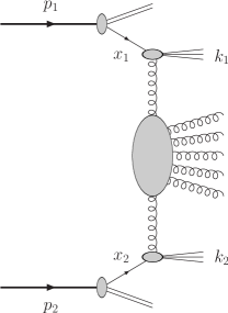
Figure 1: Schematic representation of the Mueller-Navelet jet production.

We consider the process $\rm{proton}(p_{1})+\rm{proton}(p_{2})\to\rm{jet}(k_{1})+\rm{jet}(k_{2})+X$. Introducing the Sudakov decomposition ($s=2p_{1}\cdot p_{2}$),

$$k_{1}=\alpha_{1}p_{1}+\frac{\vec{k}_{1}^{\>2}}{\alpha_{1}s}p_{2}+k_{1,\perp}\;,\;\;\;k_{1,\perp}^{2}=-\vec{k}_{1}^{\>2}\;,$$

$$k_{2}=\alpha_{2}p_{2}+\frac{\vec{k}_{2}^{\>2}}{\alpha_{2}s}p_{1}+k_{2,\perp}\;,\;\;\;k_{2,\perp}^{2}=-\vec{k}_{2}^{\>2}\;,$$

we take the kinematics when jet transverse momenta are large, $\vec{k}_{1}^{\>2}\sim\vec{k}_{2}^{\>2}\gg\Lambda_{\rm QCD}^{2}$, and there is a large rapidity gap between jets, $\Delta y=\ln\frac{\alpha_{1}\alpha_{2}s}{|\vec{k}_{1}||\vec{k}_{2}|}$, which requires large c.m. energy of the proton collisions, $s=2p_{1}\cdot p_{2}\gg\vec{k}_{1,2}^{\>2}$. In the perturbative QCD description of the process, the hard scale is provided by the jet transverse momenta, $Q^{2}\sim\vec{k}_{1,2}^{2}\gg\Lambda_{\rm QCD}^{2}$; moreover, we neglect power-suppressed contributions $\sim 1/Q$, thus allowing the use of leading-twist PDFs, $f_{g}(x)$ and $f_{q}(x)$. We still need to resum the QCD perturbative series, according to DGLAP [1], $\sum_{n}a_{n}(\alpha_{s}^{n}\ln^{n}Q^{2}+b_{n}\alpha_{s}^{n}\ln^{n-1}Q^{2})$ and BFKL [2], $\sum_{n}(c_{n}\alpha_{s}^{n}\ln^{n}s+d_{n}\alpha_{s}^{n}\ln^{n-1}s)$. Mueller and Navelet [3] proposed that, for $\Delta y\gg 1$, the BFKL approach is more adequate and leads to a faster energy dependence and more decorrelation in the relative jet azimuthal angle $\phi=\phi_{1}-\phi_{2}-\pi$.

In the BFKL approach, valid in the Regge limit $s\rightarrow\infty$, the total cross section of a hard process $A+B\to X$, via the optical theorem, $\sigma=\frac{\rm{Im}_{s}{\cal A}}{s}$, can be written as the convolution of the Green’s function of two interacting Reggeized gluons and of the impact factors of the colliding particles. This is valid both in the LLA (resummation of all terms $(\alpha_{s}\ln s)^{n}$) and in the NLA (resummation of all terms $\alpha_{s}(\alpha_{s}\ln s)^{n}$). In formulae,

$${\rm Im}_{s}{\cal A}=\frac{s}{(2\pi)^{D-2}}\!\int\!\frac{d^{D-2}\vec{q}_{1}}{\vec{q}_{1}^{\,\,2}}\Phi_{A}(\vec{q}_{1},s_{0})\!\int\!\frac{d^{D-2}\vec{q}_{2}}{\vec{q}_{2}^{\,\,2}}\Phi_{B}(-\vec{q}_{2},s_{0})\!\int\limits^{\delta+i\infty}_{\delta-i\infty}\!\frac{d\omega}{2\pi i}\left(\frac{s}{s_{0}}\right)^{\omega}G_{\omega}(\vec{q}_{1},\vec{q}_{2})\;.$$

The Green’s function is process-independent and is determined through the BFKL equation,

$$\omega\,G_{\omega}(\vec{q}_{1},\vec{q}_{2})=\delta^{D-2}(\vec{q}_{1}-\vec{q}_{2})+\int d^{D-2}\vec{q}\,K(\vec{q}_{1},\vec{q})\,G_{\omega}(\vec{q},\vec{q}_{1})\;,$$

whereas impact factors are process-dependent and only very few of them have been calculated in the NLA. For the process under consideration, the starting point is provided by the impact factors for colliding partons [4, 5] (see Fig. 2).

Figure 2: Schematic representation of quark (left) and gluon (right) impact factors.

In the LLA one needs leading-order (LO) impact factors, which take contribution only from a one-particle intermediate state in the parton-Reggeon collision; in the NLA one needs next-to-LO (NLO) impact factors, which take contributions from virtual corrections (one-particle intermediate states) and real particle production (two-particle intermediate states). The steps to get the quark(gluon) jet vertex from the quark(gluon) parton impact factor are: (1) open one of the integrations over the phase space of the intermediate state to allow one parton to generate the jet, (2) take the convolution with PDFs, $\sum_{a=q,\bar{q}}f_{a}\otimes({\rm quark\ jet\ vertex})+f_{g}\otimes({\rm gluon\ jet\ vertex})$, (3) project onto the eigenfunctions of the LO BFKL kernel, i.e. transfer to the $(\nu,n)$-representation

$$\Phi(\nu,n)=\int d^{2}\vec{q}\,\frac{\Phi(\vec{q})}{\vec{q}^{\,\,2}}\frac{1}{\pi\sqrt{2}}\left(\vec{q}^{\,\,2}\right)^{\gamma-\frac{n}{2}}\left(\vec{q}\cdot\vec{l}\,\,\right)^{n}\;,\;\;\;\;\;\gamma=i\nu-\frac{1}{2}\;,\;\;\;\;\;\vec{l}^{\>2}=0\;.$$

The NLO jet vertices have been calculated in the transverse momentum space (no step (3)) in [6] and cross-checked in [7]. They are given by complicated expression, to be transferred numerically to the $(\nu,n)$-representation, as it was done in [8], where they were used to study Mueller-Navelet jets in the NLA with LHC kinematics.

Here we want to sketch the derivation of an approximated expression for jet vertices, valid for jets with small aperture of the cone in the pseudorapidity - azimuthal angle plane. The details of the calculation are given in [9].

2 Jet definition, small-cone approximation (SCA) and outline of the calculation

In the LO we have a one-particle intermediate state and the kinematics of the produced parton $a$ is completely fixed by the jet kinematics (see Fig. 3).

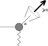
Figure 3: Parton-Reggeon collision, the jet is formed by a single parton.

In the NLO, when real corrections are considered, we have two-particle intermediate states. Then, we can have the following cases: (i) the parton $a$ generates the jet, while the parton $b$ can have arbitrary kinematics, provided that it lies outside the jet cone; (ii) similarly with $a\leftrightarrow b$; (iii) the two partons $a$ and $b$ both generate the jet (see Fig. 4(left)).

The case in which one parton (say $a$) generates the jet and the other parton is outside the jet cone can also be written as the contribution when the parton $a$ is produced with the same jet kinematics while the parton $b$ can have any kinematics (inclusive jet production by the parton $a$) minus the contribution when the parton $b$ lies inside the jet cone (see Fig. 4(right)).

The SCA [10] means that all cones which appear in the jet definition given above are to be taken with aperture (in the pseudorapidity - azimuthal angle plane) smaller than a fixed value $R$. For $s\sim Q^{2}$, very good agreement between SCA and Monte Carlo calculations was found for cone sizes up to $R=0.7$ [10].

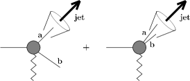
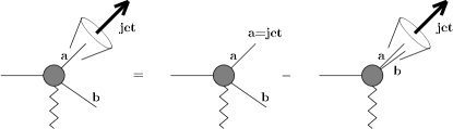
Figure 4: (Left) Parton-Reggeon collision, two partons are produced and the jet is formed either by one of the partons or by both partons. (Right) The production of the jet by one parton when the second one is outside the cone can be seen as the inclusive production minus the contribution when the second parton is inside the cone.

For the jet vertex in the LLA the starting point is given by the inclusive LO parton impact factors, $\Phi_{q}=g^{2}\frac{\sqrt{N^{2}-1}}{2N}$ and $\Phi_{g}=\frac{C_{A}}{C_{F}}\Phi_{q}$. Then we have to open the integration over the one-particle intermediate state, i.e. introduce suitable delta functions, and take the convolution with the PDFs, getting ($\alpha$ and $\vec{k}$ are the jet kinematic variables)

$$\frac{d\Phi^{J}}{\vec{q}^{\,\,2}}={\cal C}\int\,d\alpha\frac{d^{2}\vec{k}}{\vec{k}^{\,2}}\,dx\,\delta^{(2)}\left(\vec{k}-\vec{q}\right)\delta(\alpha-x)\left(\frac{C_{A}}{C_{F}}f_{g}(x)+\sum_{a=q,\bar{q}}f_{a}(x)\right)\;.$$

This expression can be used to construct the collinear and QCD coupling counterterms in the NLA, arising when the renormalization of the PDFs and of the QCD coupling are taken into account.

For the jet vertex in the NLA, we separate the cases of quark- and gluon-iniziated subprocesses. For incoming quark, we have the following contributions: (a) virtual corrections, (b) real corrections from the quark-gluon state. The contribution (b) can be separated into the following pieces: (b₁) both quark and gluon generate the jet, (b₂) gluon inclusive jet generation minus gluon inclusive jet generation with the quark in the jet cone, (b₃) quark inclusive jet generation minus quark inclusive jet generation with the gluon in the jet cone. For incoming gluon, we have the following contributions: (a) virtual corrections, (b) real corrections from quark-antiquark state, (c) real corrections from two-gluon state. The contribution (b) can be separated into the following pieces: (b₁) both quark and antiquark generate the jet, (b₂) (anti)quark inclusive jet generation minus (anti)quark inclusive jet generation with the antiquark(quark) in the jet cone. The contribution (c) can be separated into the following pieces: (c₁) both gluons generate the jet, (c₂) gluon inclusive jet generation minus gluon inclusive jet generation with the other gluon in the jet cone.

The final result for the jet vertex (see [9]) in the $(\nu,n)$-representation is free of IR and UV divergences and is of the form $A\ln R+B+{\cal O}(R^{2})$, as discussed in [11].

3 Summary

The NLO vertex for the forward production of a high-$p_{T}$ jet from an incoming quark or gluon, emitted by a proton, has been calculated in the SCA. The result has been presented in the so called $(\nu,n)$-representation, which turns to be very convenient for numerical implementation, as discussed in [12]. Besides Mueller-Navelet jets, the vertex can be used also for forward-jet electroproduction, $\gamma^{*}p\to{\rm jet}+X$, in combination with the NLO photon impact factor [13].

References

- [1] V.N. Gribov, L.N. Lipatov, Sov. J. Nucl. Phys. 15 (1972) 438; G. Altarelli, G. Parisi, Nucl. Phys. B 126 (1977) 298; Y.L. Dokshitzer, Sov. Phys. JETP 46 (1977) 641.
- [2] V.S. Fadin, E.A. Kuraev, L.N. Lipatov, Phys. Lett. B 60 (1975) 50; E.A. Kuraev, L.N. Lipatov and V.S. Fadin, Zh. Eksp. Teor. Fiz. 71 (1976) 840 [Sov. Phys. JETP 44 (1976) 443]; 72 (1977) 377 [45 (1977) 199]; Ya.Ya. Balitskii and L.N. Lipatov, Sov. J. Nucl. Phys. 28 (1978) 822.
- [3] A.H. Mueller, H. Navelet, Nucl. Phys. B 282 (1987) 727.
- [4] V.S. Fadin, R. Fiore, M.I. Kotsky and A. Papa, Phys. Rev. D 61 (2000) 094005; Phys. Rev. D 61 (2000) 094006.
- [5] M. Ciafaloni and G. Rodrigo, JHEP 0005 (2000) 042.
- [6] J. Bartels, D. Colferai and G.P. Vacca, Eur. Phys. J. C 24 (2002) 83; Eur. Phys. J. C 29 (2003) 235;
- [7] F. Caporale, D.Yu. Ivanov, B. Murdaca, A. Papa and A. Perri, JHEP 1202 (2012) 101.
- [8] D. Colferai, F. Schwennsen, L. Szymanowski, S. Wallon, JHEP 1012 (2010) 026.
- [9] D.Yu. Ivanov and A. Papa, arXiv:1202.1082.
- [10] B. Jäger, M. Stratmann, W. Vogelsang, Phys. Rev. D 70 (2004) 034010.
- [11] M. Furman, Nucl. Phys. B 197 (1982) 413.
- [12] D.Yu. Ivanov and A. Papa, Nucl. Phys. B 732 (2006) 183; Eur. Phys. J. C 49 (2007) 947; F. Caporale, A. Papa and A. Sabio Vera, Eur. Phys. J. C 53 (2008) 525.
- [13] G. Chirilli, these proceedings and references therein.