ODE Solvers Using Band-limited Approximations

Abstract.

We use generalized Gaussian quadratures for exponentials to develop a new ODE solver. Nodes and weights of these quadratures are computed for a given bandlimit $c$ and user selected accuracy $\epsilon$, so that they integrate functions $e^{ibx}$, for all $|b|\leq c$, with accuracy $\epsilon$. Nodes of these quadratures do not concentrate excessively near the end points of an interval as those of the standard, polynomial-based Gaussian quadratures. Due to this property, the usual implicit Runge-Kutta (IRK) collocation method may be used with a large number of nodes, as long as the method chosen for solving the nonlinear system of equations converges. We show that the resulting ODE solver is symplectic and demonstrate (numerically) that it is A-stable. We use this solver, dubbed Band-limited Collocation (BLC-IRK), for orbit computations in astrodynamics. Since BLC-IRK minimizes the number of nodes needed to obtain the solution, in this problem we achieve speed close to that of the traditional explicit multistep methods.

1. Introduction

Current methods for solving ODEs, be that multistep or Runge-Kutta, are based on polynomial approximations of functions. However, both classical and recent results [26, 14, 25, 27, 1, 2, 3, 18] indicate that in many situations band-limited functions provide a better tool for numerical integration and interpolation of functions than the traditional polynomials. We construct a new method for solving the initial value problem for Ordinary Differential Equations (ODEs) using band-limited approximations and demonstrate certain advantages of such approach. As an example, we consider orbit computations in astrodynamics as a practical application for the new ODE solver as well as a gauge to ascertain its performance.

It is well-known that choosing between equally spaced and unequally spaced nodes on a specified time interval, in other words, choosing a multistep vs a collocation based Runge-Kutta method, results in significantly different properties of ODE solvers. For example, multistep schemes have $\left\{\mathcal{R}e(z)\leq 0,\,\,z\in\mathbb{C}\right\}$ as the region of absolute stability (A-stable) only if their order does not exceed $2$, the so-called Dahlquist barrier. In contrast, an A-stable implicit Runge-Kutta (IRK) scheme may be of arbitrary order. A class of A-stable IRK schemes uses the Gauss-Legendre quadrature nodes on each time interval and the order of such methods is $2\nu$, where $\nu$ is the number of nodes (see, e.g., [11]). A-stability assures that growth and decay of numerical solutions exactly mimics that of the analytic solutions of the test problem which, in turn, implies that the choice of step size involves only accuracy consideration.

Another numerical property of interest, that of preservation of volume in the phase space, identifies symplectic integrators. Symplectic integrators preserve a particular conserved quantity of Hamiltonian systems as well as an approximate Hamiltonian. In problems of orbit determination, a symplectic integrator would maintain the correct orbit more or less indefinitely with the error accumulating only in a position along that orbit, thus closely reproducing a particular behavior of analytic solutions of nonlinear Hamiltonian systems. We note that IRK schemes which use the Gauss-Legendre nodes are symplectic (see, e.g., [11]).

While IRK schemes with the Gauss-Legendre nodes provide an excellent discretization of a system of ODEs, using many such nodes on a specified time interval is not practical. The nodes of the Gauss-Legendre quadratures (as well as any other polynomial based Gaussian quadratures) accumulate rapidly towards the end points of an interval. A heuristic reason for such accumulation is that these quadratures have to account for a possible rapid growth of polynomials near the boundary.

In this paper we demonstrate that, within IRK collocation methods, quadratures based on polynomials may be replaced by quadratures for band-limited exponentials. The nodes of these quadratures do not accumulate significantly toward the end points of an interval (a heuristic reason for an improved arrangement of nodes is that the exponentials do not grow anywhere within the interval). Our method addresses numerical integration of ODEs whose solutions are well approximated by band-limited exponentials. Band-limited exponentials have been successfully used in problems of wave propagation [2] (see also [20]), where it is natural to approximate solutions by band-limited functions. While solutions of ODEs are typically well approximated by band-limited exponentials as well, there may be exceptions since some ODEs may have polynomial solutions. In such cases the use of polynomial based quadratures may be more efficient.

Unlike the classical Gaussian quadratures for polynomials that integrate exactly a subspace of polynomials up to a fixed degree, the Gaussian type quadratures for exponentials use a finite set of nodes to integrate an infinite set of functions, namely, $\left\{e^{ibx}\right\}_{\left|b\right|\leq c}$ on the interval $\left|x\right|\leq 1$. As there is no way to accomplish this exactly, these quadratures are constructed so that all exponentials with $|b|\leq c$ are integrated with accuracy of at least $\epsilon$, where $\epsilon$ is arbitrarily small but finite. Such quadratures were constructed in [1] and, via a different approach in [27] (see also [19]). As observed in [2], quadrature nodes of this type do not concentrate excessively toward the end of the interval. The density of nodes increases toward the end points of the interval only by a factor that depends on the desired accuracy $\epsilon$ but not on the overall number of nodes.

Using quadratures to integrate band-limited exponentials with bandlimit $2c$ and accuracy $\epsilon^{2}$, we naturally arrive at a method for interpolation of functions with bandlimit $c$ and accuracy $\epsilon$ (see [27, 1]). It turns out that the nodes and weights of quadratures to interpolate with accuracy $\epsilon\approx 10^{-15}$ can, in fact, be constructed using only the standard double precision machine arithmetic. However, generating the integration matrix for the new double precision BLC-IRK method requires using quadruple precision in the intermediate calculations. Importantly, once generated, the quadratures and the integration matrix are applied using only the standard double precision.

While analytically the classical Gauss-Legendre quadratures for polynomials are exact, in practice their accuracy is limited by the machine precision. By choosing (interpolation) accuracy $\epsilon\approx 10^{-15}$, our integrator is effectively “exact” within the double precision of machine arithmetic. Remarkably, using a particular construction of the integration matrix, we show that BLC-IRK method is (exactly) symplectic and, with high accuracy, A-stable. This result was unexpected and indicates that properties of approximate quadratures for band-limited exponentials need to be explored further.

While IRK schemes require solving a system of nonlinear equations at each time step, it does not automatically imply that such schemes are always computationally more expensive than explicit schemes. In the environment where the cost of function evaluation is high, the balance between the necessary iteration with fewer nodes of an implicit scheme vs significantly greater number of nodes of an explicit scheme (but no iteration), may tilt towards an implicit scheme. In problems of astrodynamics, we use an additional observation that most iterations can be performed with an inexpensive (low fidelity) gravity model, making implicit schemes with a large number of nodes per time interval practical. We select the problem of orbit determination as an example where our approach is competitive with numerical schemes that are currently in use (see [4, 5]). We take advantage of the reduced number of function calls to the full gravity model in a way that appears difficult to replicate using alternative schemes.

In order to accelerate solving a system of nonlinear equations, we modify the scheme by explicitly exponentiating the linear part of the force term. For the problem of orbit computations this modification accelerates convergence of iterations by (effectively) makes use of the fact that the system is of the second order. So far we did not study possible acceleration of iterations using spectral deferred correction approach as in [8, 16, 10, 12].

We start by providing background information on quadratures for band-limited functions in Section 2. We then describe BLC-IRK method in Section 3 (with some details deferred to Appendix). In Section 4 we detail our algorithm and provide examples.

2. Preliminaries: quadratures for band-limited functions

2.1. Band-limited functions as a replacement of polynomials

The quadratures constructed in [27, 1, 19] break with the conventional approach of using polynomials as the fundamental tool in analysis and computation. The approach based on polynomial approximations has a long tradition and leads to such notions as the order of convergence of numerical schemes, polynomial based interpolation, and so on. Recently, an alternative to polynomial approximations has been developed; it turns out that constructing quadratures for band-limited functions, e.g., exponentials $e^{ibx}$, with $|b|\leq c$, where $c$ is the bandlimit, in many cases leads to significant improvement in performance of algorithms for interpolation, estimation and solving partial differential equations [2, 20, 13].

2.2. Bases for band-limited functions

It is well-known that a function whose Fourier Transform has compact support can not have compact support itself unless it is identically zero. On the other hand, in physics duration of all signals is finite and their frequency response for all practical purposes is also band-limited. Thus, it is important to identify classes of functions which are essentially time and frequency limited. Towards this end, it is natural to analyze an operator whose effect on a function is to truncate it both in the original and the Fourier domains. Indeed, this has been the topic of a series of seminal papers by Slepian, Landau and Pollak, [26, 14, 15, 22, 23, 24, 25], where they observed (inter alia) that the eigenfunctions of such operator (see (2.2) below) are the Prolate Spheroidal Wave Functions (PSWFs) of classical Mathematical Physics.

While periodic band-limited functions may be expanded into Fourier series, neither the Fourier series nor the Fourier integral may be used efficiently for non-periodic functions on intervals. This motivates us to consider a class of functions (not necessarily periodic) admitting a representation via exponentials $\left\{e^{ibx}\right\}_{\left|b\right|\leq c}$, $x\in\left[-1,1\right]$, with a fixed parameter $c$ (bandlimit). Following [1], let us consider the linear space of functions

$$\mathcal{E}_{c}=\left\{u\!\in\!L^{\infty}(\left[-1,1\right])\ \left|\right.\ u(x)=\sum_{k\in\mathbb{Z}}a_{k}e^{icb_{k}x}:\left\{a_{k}\right\}{}_{k\in\mathbb{Z}}\!\in\!l^{1},\ b_{k}\!\in\left[-1,1\right]\right\}.$$

Given a finite accuracy $\epsilon$, we represent the functions in $\mathcal{E}_{c}$ by a fixed set of exponentials $\left\{e^{ic\tau_{k}x}\right\}_{k=1}^{M}$, where $M$ is as small as possible. It turns out that by finding quadrature nodes $\left\{\tau_{k}\right\}{}_{k=1}^{M}$ and weights $\left\{w_{k}\right\}{}_{k=1}^{M}$ for exponentials with bandlimit $2c$ and accuracy $\epsilon^{2}$, we in fact obtain (with accuracy $\epsilon$) a basis for $\mathcal{E}_{c}$ with bandlimit $c$ [1].

The generalized Gaussian quadratures for exponentials are constructed in [1] (see [27] and [19] for different constructions), which we summarize as

Lemma 1.

For $c>0$ and any $\epsilon>0$, there exist nodes $-1<\tau_{1}<\tau_{2}<\dots<\tau_{M}<1$ and corresponding weights $w_{k}>0$, such that for any $x\in\left[-1,1\right]$,

(2.1) $$\left|\int_{-1}^{1}e^{ictx}\ dt-\sum_{k=1}^{M}w_{k}e^{ic\tau_{k}x}\right|<\epsilon,$$

where the number of nodes, $M$, is (nearly) optimal. The nodes and weights maintain the natural symmetry, $\tau_{k}=-\tau_{M-k+1}$ and $w_{k}=w_{M-k+1}$.

Remark 2.

The construction in [1] is more general and yields quadratures for band-limited exponentials integrated with a weight function. If the weight function is $1$ as in Lemma 1, then the approach in [1] identifies the nodes of the generalized Gaussian quadratures in (2.1) as zeros of the Discrete Prolate Spheroidal Wave Functions (DPSWFs) [24], corresponding to small eigenvalues.

Next we consider band-limited functions,

$$\mathcal{B}_{c}=\{f\in L^{2}(\mathbb{R})\,\left|\right.\hat{f}(\omega)=0\,\,\mbox{for}\,\,\left|\omega\right|\geq c\},$$

and briefly summarize some of the results in [26, 14, 15, 22, 25]. Let us define the operator $F_{c}:\,\,L^{2}\left[-1,1\right]\rightarrow L^{2}\left[-1,1\right]$,

(2.2) $$F_{c}(\psi)(\omega)=\int_{-1}^{1}e^{icx\omega}\psi(x)dx,$$

where $c>0$ is the bandlimit. We also consider the operator $Q_{c}=\frac{c}{2\pi}F_{c}^{*}F_{c}$,

(2.3) $$Q_{c}(\psi)(y)=\frac{1}{\pi}\int_{-1}^{1}\frac{\sin(c(y-x))}{y-x}\psi(x)\,\,dx.$$

The eigenfunctions $\psi_{0}^{c},\psi_{1}^{c},\psi_{2}^{c},\cdots$ of $Q_{c}$ coincide with those of $F_{c}$, and the eigenvalues $\mu_{j}$ of $Q_{c}$ are related to the eigenvalues $\lambda_{j}$ of $F_{c}$ as

(2.4) $$\mu_{j}=\frac{c}{2\pi}|\lambda_{j}|^{2},\,\,\,\,\,j=0,1,2,\dots.$$

While all $\mu_{j}<1$, $j=0,1,\dots$, for large $c$ the first approximately $2c/\pi$ eigenvalues $\mu_{j}$ are close to $1$. They are followed by $\mathcal{O}(\log c)$ eigenvalues which decay exponentially fast forming a transition region; the rest of the eigenvalues $\mu_{j}$ are very close to zero.

The key result in [26] states that there exists a strictly increasing sequence of real numbers $\gamma_{0}<\gamma_{1}\dots$, such that $\psi_{j}^{c}$ are eigenfunctions of the differential operator,

(2.5) $$L_{c}\psi_{j}^{c}\equiv\left(-(1-x^{2})\,\frac{d^{2}}{dx^{2}}\,+\,2x\frac{d}{dx}\,+\,c^{2}x^{2}\right)\psi_{j}^{c}(x)\,=\,\gamma_{j}\psi_{j}^{c}(x)\,.$$

The eigenfunctions of $L_{c}$ have been known as the angular Prolate Spheroidal Wave Functions (PSWF) before the connection with (2.2) was discovered in [26] by demonstrating that $L_{c}$ and $F_{c}$ commute. We note that if $c\to 0$, then it follows from (2.5) that, in this limit, $\psi_{j}^{c}$ become the Legendre polynomials. In many respects, PSWFs are strikingly similar to orthogonal polynomials; they are orthonormal, constitute a Chebychev system, and admit a version of Gaussian quadratures [27].

Since the space $\mathcal{E}_{c}$ is dense in $\mathcal{B}_{c}$ (and vice versa) [1], we note that the quadratures in [27] may potentially be used for the purposes of this paper as well (the nodes of the quadratures in [27] and those used in this paper are close but are not identical). Importantly, given accuracy $\epsilon$, the functions $\psi_{0}^{c},\psi_{1}^{c},\psi_{2}^{c},\cdots,\psi_{M-1}^{c}$ may be used as a basis for interpolation on the interval $\left[-1,1\right]$ with $\tau_{1},\tau_{2},\cdots,\tau_{M}$ as the interpolation nodes, provided that these are quadrature nodes constructed for the bandlimit $2c$ and accuracy $\epsilon^{2}$. Given functions $\psi_{0}^{c},\psi_{1}^{c},\psi_{2}^{c},\cdots,\psi_{M-1}^{c}$, we can construct an analogue of the Lagrange interpolating polynomials, $R_{k}^{c}(x)=\sum_{j=0}^{M-1}\alpha_{kj}\psi_{j}^{c}(x)$, $x\in\left[-1,1\right]$, by solving

(2.6) $$\delta_{kl}=R_{k}^{c}(\tau_{l})=\sum_{j=0}^{M-1}\alpha_{kj}\psi_{j}^{c}(\tau_{l})$$

for the coefficients $\alpha_{kj}$. The matrix $\psi_{j}^{c}(\tau_{l})$ in (2.6) is well conditioned.

A well-known problem associated with the numerical use of orthogonal polynomials is concentration of their roots near the ends of the interval. Let us consider the ratio

(2.7) $$r(M,\epsilon)=\frac{\tau_{2}-\tau_{1}}{\tau_{\lfloor M/2\rfloor}-\tau_{\lfloor M/2\rfloor-1}},$$

where “$\lfloor M/2\rfloor$” denotes the least integer part, and look at it as a function of $M$. Observing that the distance between nodes of Gaussian quadratures for exponentials changes monotonically from the middle of an interval toward its end points, and that the smallest distance occurs between the nodes closest to the end point, the ratio (2.7) may be used as a measure of node accumulation. For example, the distance between the nodes near the end points of the standard Gaussian quadratures for polynomials decreases as $\mathcal{O}(1/M^{2})$, so that we have $r(M,\epsilon)=\mathcal{O}(1/M)$, where $M$ is the number of nodes. In Figure 2.1 we illustrate the behavior of $r(M,\epsilon)$ for the nodes of quadratures for band-limited exponentials. This ratio approaches a constant that depends on the accuracy $\epsilon$ but does not depend on the number of nodes.

Another important property of quadratures for exponentials emerges if we compare the critical sampling rate of a smooth periodic function, to that of smooth non-periodic function defined on an interval. Considering bandlimit $c$ as a function of the number of nodes, $M$, and the desired accuracy $\epsilon$, we observe that the oversampling factor,

$$\alpha(M,\epsilon)=\frac{\pi M}{c(M,\epsilon)}>1,$$

approaches $1$ for large M. We recall that in the case of the Gaussian quadratures for polynomials, this oversampling factor approaches $\frac{\pi}{2}$ rather than $1$ (see e.g. [9]).

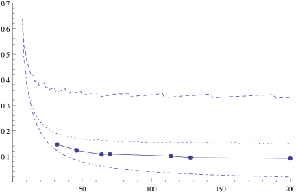
Figure 2.1. The ratio $r(M,\epsilon)$ in (2.7) as a function of the number of nodes $M$ and interpolation accuracy $\epsilon\approx 10^{-3.5}$ (top curve, dashed), $\epsilon\approx 10^{-8.5}$ (middle curve, dotted) and $\epsilon\approx 10^{-13}$ (middle curve, solid). The dots on the solid curve indicate the number of nodes of quadratures used in our numerical experiments. The bottom curve shows this ratio for the Gauss-Legendre nodes.

2.3. Interpolating bases for band-limited functions

A basis of interpolating band-limited functions for the bandlimit $c$ and accuracy $\epsilon$ plays the same role in the derivation of a system of nonlinear equations for solving ODEs as the bases of Lagrange interpolating polynomials defined on the Gauss-Legendre nodes. While (2.6) relies on available solutions of the differential equation (2.5), interpolating basis functions may also be obtained by solving the integral equation (2.2) (see [1, 19]).

We start by first constructing a quadrature for the bandlimit $2c>0$ and accuracy threshold $\epsilon^{2}>0$, yielding $M$ nodes $\left\{\tau_{m}\right\}_{m=1}^{M}$ and weights $\left\{w_{m}\right\}_{m=1}^{M}$. For the inner product of two functions $f,g\in\mathcal{E}_{c}$, we have

$$\left|\int_{-1}^{1}f(t)g(t)dt-\sum_{m=1}^{M}w_{m}f(\tau_{m})g(\tau_{m})\right|\leq\epsilon^{2}.$$

Following [1], we discretize (2.2) using nodes $\left\{\tau_{m}\right\}_{m=1}^{M}$ and weights $\left\{w_{m}\right\}_{m=1}^{M}$ and obtain an algebraic eigenvalue problem,

(2.8) $$\sum_{l=1}^{M}w_{l}e^{ic\tau_{m}\tau_{l}}\mathbf{\Psi}_{j}(\tau_{l})=\eta_{j}\mathbf{\Psi}_{j}(\tau_{m}).$$

The approximate PSWFs on $[-1,1]$ are then defined consistent with (2.2) as

(2.9) $$\Psi_{j}(x)=\frac{1}{\eta_{j}}\sum_{l=1}^{M}w_{l}e^{icx\tau_{l}}\mathbf{\Psi}_{j}(\tau_{l}),$$

where $\eta_{j}$ are the eigenvalues and $\mathbf{\Psi}_{j}(\tau_{l})$ the eigenvectors in (2.8). Following [1], we then define the interpolating basis for band-limited functions as

(2.10) $$R_{k}(x)=\sum_{l=1}^{M}r_{kl}e^{ic\tau_{l}x},\,\,\,\,k=1,\ldots,M,$$

where

(2.11) $$r_{kl}=\sum_{j=1}^{M}w_{k}\mathbf{\Psi}_{j}(\tau_{k})\frac{1}{\eta_{j}}\mathbf{\Psi}_{j}(\tau_{l})w_{l}.$$

It is shown in [1] that the functions $R_{k}(x)$ are interpolating, $R_{k}(\tau_{l})=\delta_{kl}$.

3. BLC-IRK method

3.1. Discretization of Picard integral equation

We consider the initial value problem for a system of ODEs,

$$\mathbf{y}^{\prime}=\mathbf{f}(t,\mathbf{y}),\,\,\,\,\,\mathbf{y}(0)=\mathbf{y_{0}},$$

or, equivalently,

(3.1) $$\mathbf{y}(t)=\mathbf{y_{0}}+\int_{0}^{t}\mathbf{f}(s,\mathbf{y}(s))\ ds.$$

It is sufficient to discretize (3.1) on the interval $\left[0,t\right]$ since, by shifting the time variable, the initial condition may always be set at $t=0$. We require

$$\mathbf{y}^{\prime}(t\tau_{j})=\mathbf{f}(t\tau_{j},\mathbf{y}(t\tau_{j})),\,\,\,j=1,\dots,M,$$

where $\{\tau_{j}\}_{j=1}^{M}$ are Gaussian nodes for band-limited exponentials on $[0,1]$ (constructed for an appropriate bandlimit $c$ and accuracy $\epsilon$). We approximate

(3.2) $$\|\mathbf{f}(t\tau,\mathbf{y}(t\tau))-\sum_{j=1}^{M}\mathbf{f}(t\tau_{j},\mathbf{y}(t\tau_{j}))R_{j}(\tau)\|\leq\epsilon,\,\,\,\,\tau\in\left[0,1\right]$$

where $R_{j}(\tau)$ are interpolating basis functions associated with these quadratures and briefly described in Section 2.3 (see [1, 2] for details). Using (3.2), we replace $\mathbf{f}$ in (3.1) and evaluate $\mathbf{y}(t\tau)$ at the quadrature nodes yielding a nonlinear system,

$$\mathbf{y}(t\tau_{k}) = \mathbf{y_{0}}+\sum_{j=1}^{M}\mathbf{f}(t\tau_{j},\mathbf{y}(t\tau_{j}))\int_{0}^{\tau_{k}}R_{j}(s)ds$$

$$= \mathbf{y_{0}}+\sum_{j=1}^{M}S_{kj}\mathbf{f}(t\tau_{j},\mathbf{y}(t\tau_{j})),$$

where $S_{kj}=\int_{0}^{\tau_{k}}R_{j}(s)ds$ is the integration matrix and $k=1,\dots M$. After solving for $\{\mathbf{y}(t\tau_{j})\}_{j=1}^{M}$, we have from (3.1)

(3.4) $$\mathbf{y}(t)=\mathbf{y_{0}}+\sum_{j=1}^{M}w_{j}\mathbf{f}(t\tau_{j},\mathbf{y}(t\tau_{j})),$$

where $\{w_{j}\}_{j=1}^{M}$ are the quadrature weights. The result is an implicit Runge-Kutta method (IRK) where the usual Gauss-Legendre quadratures are replaced by Gaussian quadratures for band-limited exponentials.

The nodes, weights, and the entries of the integration matrix are typically organized in the Butcher tableau,

$\tau$	$S$
	$w^{t}$

.

Unlike in the standard IRK method based on Gauss-Legendre quadratures, we solve (3.1) on a time interval containing a large number of quadrature nodes, since these nodes do not concentrate excessively near the end points. This implies that the interval $\left[0,t\right]$ may be selected to be large in comparison with the usual choices in RK methods.

3.2. Exact Linear Part

In many problems (including that of orbit computations in astrodynamics), the right hand side of the ODE, $\mathbf{f}(t,\mathbf{y})$, may be split into a linear and nonlinear part,

$$\mathbf{f}(t,\mathbf{y}(t))=\mathbf{L}\mathbf{y}(t)+\mathbf{g}(t,\mathbf{y}(t)),$$

so that the integral equation (3.1) may be written as

(3.5) $$\mathbf{y}(t)=e^{tL}\mathbf{y_{0}}+\int_{0}^{t}e^{(t-s)\mathbf{L}}\mathbf{g}(s,\mathbf{y}(s))\ ds.$$

If the operator $e^{t\mathbf{L}}$ can be computed efficiently, this formulation leads to savings when solving the integral equation iteratively.

We discretize (3.5) by using (3.2) and obtain

(3.6) $$\mathbf{y}(t\tau_{k}) = e^{t\tau_{k}\mathbf{L}}\mathbf{y_{0}}+\sum_{j=1}^{M}e^{t(\tau_{k}-\tau_{j})\mathbf{L}}\mathbf{g}(t\tau_{j},\mathbf{y}(t\tau_{j}))\int_{0}^{\tau_{k}}R_{j}(s)ds$$

$$= e^{t\tau_{k}\mathbf{L}}\mathbf{y_{0}}+\sum_{j=1}^{M}S_{kj}e^{t(\tau_{k}-\tau_{j})\mathbf{L}}\mathbf{g}(t\tau_{j},\mathbf{y}(t\tau_{j}))$$

where $S_{kj}=\int_{0}^{\tau_{k}}R_{j}(s)ds$. We note that (3.1) is a special case of (3.6) with $\mathbf{L}=0$ and $\mathbf{g}=\mathbf{f}$.

3.3. Symplectic integrators

Following [21], let us introduce matrix $\mathcal{M}=\{m_{kj}\}_{k,j=1}^{M}$ for an $M$-stage IRK scheme,

(3.7) $$m_{kj}=w_{k}S_{kj}+w_{j}S_{jk}-w_{k}w_{j},$$

where the weights $w=\{w_{k}\}_{k=1}^{M}$ and the integration matrix $S=\{S_{kj}\}_{k,j=1}^{M}$ define the Butcher’s tableau for the method.

It is shown in [21] that

Theorem 3.

If matrix $\mathcal{M}=0$ in (3.7), then an $M$-stage IRK scheme is symplectic.

This condition, $\mathcal{M}=0$, is satisfied for the Gauss-Legendre RK methods, see e.g. [6, 21]. We enforce this condition for BLC-IRK method by an $\mathcal{O}(\epsilon^{2})$ modification of the weights and of the integration matrix. For convenience, in what follows, we consider the band-limited exponentials and integration matrix on the interval $\left[-1,1\right]$ rather than on the interval $\left[0,1\right]$ usually used for ODEs.

Proposition 4.

Let $\{\tau_{j}\}_{j=1}^{M}$ and $\{w_{j}\}_{j=1}^{M}$ be quadrature nodes and weights for the bandlimit $2c$ and accuracy $\epsilon^{2}$. Consider interpolating basis functions on these quadrature nodes, $R_{k}(\tau)$, $R_{k}(\tau_{j})=\delta_{kj}$, $k,j=1,\dots,M$, and define $F_{k}(\tau)=\int_{-1}^{\tau}R_{k}(s)\ ds$. Then we have

(3.8) $$\left|\int_{-1}^{1}F_{j}(\tau)F^{\prime}_{k}(\tau)\ d\tau-\sum_{l=1}^{M}w_{l}F_{j}(\tau_{l})F^{\prime}_{k}(\tau_{l})\right|<\epsilon^{2}$$

or

$$\left|\int_{-1}^{1}\left(\int_{-1}^{\tau}R_{j}(s)\ ds\right)\ R_{k}(\tau)\ d\tau-w_{k}\int_{-1}^{\tau_{k}}R_{j}(s)\ ds\right|<\epsilon^{2},$$

and

(3.9) $$\left|\int_{-1}^{1}R_{k}(\tau)\ d\tau-\sum_{l=1}^{M}w_{l}R_{k}(\tau_{l})\right|<\epsilon^{2},$$

or

$$\left|\int_{-1}^{1}R_{k}(s)\ ds-w_{k}\right|<\epsilon^{2}.$$

Proof.

The relations in (3.8) and (3.9) is the property of the quadrature, since the bandlimit of the product $F_{j}(\tau)F^{\prime}_{k}(\tau)$ is less or equal to $2c$ and that of $R_{k}(\tau)$ is less or equal to $c$. Due to the interpolating property of $R_{k}(\tau)$, we have

(3.10) $$\sum_{l=1}^{M}w_{l}F_{j}(\tau_{l})F^{\prime}_{k}(\tau_{l})=\sum_{l=1}^{M}\left(\int_{-1}^{\tau_{l}}R_{j}(s)\ ds\right)\ w_{l}R_{k}(\tau_{l})=w_{k}\int_{-1}^{\tau_{k}}R_{j}(s)\ ds$$

and

$$\sum_{l=1}^{M}w_{l}R_{k}(\tau_{l})=w_{k}$$

Also, by definition,

$$\int_{-1}^{1}F_{j}(\tau)F^{\prime}_{k}(\tau)\ d\tau=\int_{-1}^{1}\left(\int_{0}^{\tau}R_{j}(s)\ ds\right)\ R_{k}(\tau)\ d\tau,$$

and the result follows.∎

Theorem 5.

Let $\{\tau_{j}\}_{j=1}^{M}$ be quadrature nodes of the quadrature for the bandlimit $2c$ and accuracy $\epsilon^{2}$ and $R_{k}(\tau)$, $R_{k}(\tau_{j})=\delta_{kj}$, $k,j=1,\dots,M$, the corresponding interpolating basis. Let us define weights for the quadrature as

(3.11) $$w_{k}=\int_{-1}^{1}R_{k}(\tau)d\tau$$

and the integration matrix as

(3.12) $$S_{kj}=\frac{\int_{-1}^{1}\left(\int_{-1}^{\tau}R_{j}(s)\ ds\right)\ R_{k}(\tau)\ d\tau}{w_{k}},\,\,\,k,j=1,\dots,M.$$

Then

(3.13) $$w_{k}S_{kj}+w_{j}S_{jk}-w_{k}w_{j}=0,$$

and the implicit scheme using these nodes and weights is symplectic.

Proof.

Using Proposition 4, we observe that the weights defined in (3.11) are the same (up to accuracy $\epsilon^{2}$) as those of the quadrature. The result follows by setting $F_{k}(\tau)=\int_{-1}^{\tau}R_{k}(\tau)\ d\tau$, $F^{\prime}_{k}(\tau)=R_{k}(\tau)$ and integrating by parts to obtain

$$\begin{split}w_{k}S_{kj}+w_{j}S_{jk}-w_{k}w_{j}&=\int_{-1}^{1}F_{j}(\tau)F^{\prime}_{k}(\tau)\ d\tau+\int_{-1}^{1}F_{k}(\tau)F^{\prime}_{j}(\tau)\ d\tau-w_{k}w_{j}\\ &=F_{j}(1)F_{k}(1)-w_{k}w_{j}.\end{split}$$

By the definition of the weights, we have $F_{k}(1)=w_{k}$ and, hence, $F_{j}(1)F_{k}(1)-w_{k}w_{j}=0$. ∎

3.4. Construction of the integration matrix

There are at least three approaches to compute the integration matrix. Two of them, presented in the Appendix, rely on Theorem 5 and differ in the construction of interpolating basis functions. In what appears to be a simpler approach, the integration matrix may also be obtained without computing interpolating basis functions explicitly and, instead, using a collocation condition derived below together with the symplectic condition (3.13).

We require that our method accurately solves the test problems

$$y^{\prime}=ic\tau_{m}y,\,\,\,\,\,y(-1)=e^{-ic\tau_{m}},\,\,\,m=1,\dots,M,$$

on the interval $\left[-1,1\right]$, where $\tau_{m}$ are the nodes of the quadrature. Specifically, given solutions of these test problems, $y_{m}(t)=e^{ic\tau_{m}t}$, we require that (3.1) holds at the nodes $t=\tau_{k}$ with accuracy $\epsilon$,

(3.14) $$\left|\frac{e^{ic\tau_{m}\tau_{k}}-e^{-ic\tau_{m}}}{ic\tau_{m}}-\sum_{j=1}^{M}S_{kj}e^{ic\tau_{m}\tau_{j}}\right|\leq\epsilon,\,\,\,\,m,k=1,\dots,M.$$

We then obtain the integration matrix as the solution of (3.13) satisfying an approximate collocation condition (3.14).

We proceed by observing that (3.13) suggests that the integration matrix can be split into symmetric and antisymmetric part. Defining the symmetric part of the integration matrix as

(3.15) $$T_{kj}=\frac{w_{k}w_{j}}{w_{k}+w_{j}},$$

we set

(3.16) $$S_{kj}=T_{kj}+A_{kj}w_{j},$$

and observe that it follows from (3.13) that $A_{kj}$ is antisymmetric,

$$A_{kj}+A_{jk}=0.$$

Using (3.16) and casting (3.14) as an equality, we obtain equations for the matrix entries $A_{kj}$,

(3.17) $$\sum_{j=1}^{M}A_{kj}w_{j}e^{ic\tau_{m}\tau_{j}}=\frac{e^{ic\tau_{m}\tau_{k}}-e^{-ic\tau_{m}}}{ic\tau_{m}}-\sum_{j=1}^{M}T_{kj}e^{ic\tau_{m}\tau_{j}},\,\,\,\,m,k=1,\dots,M.$$

Splitting the real and imaginary parts of the right hand side,

$$\frac{e^{ic\tau_{m}\tau_{k}}-e^{-ic\tau_{m}}}{ic\tau_{m}}-\sum_{j=1}^{M}T_{kj}e^{ic\tau_{m}\tau_{j}}=u_{km}+iv_{km},$$

we obtain

$$u_{km}=\left(\tau_{k}+1\right)\mbox{sinc}\left(c\tau_{m}(\tau_{k}+1)/2\right)\cos\left(c\tau_{m}(\tau_{k}-1)/2\right)-\sum_{j=1}^{M}T_{kj}\cos\left(c\tau_{m}\tau_{j}\right)$$

and, since $T_{kj}=T_{k\left(M-j+1\right)}$due to the symmetry of the weights, we arrive at

$$v_{km}=\left(\tau_{k}+1\right)\mbox{sinc}\left(c\tau_{m}(\tau_{k}+1)/2\right)\sin\left(c\tau_{m}(\tau_{k}-1)/2\right).$$

We also have

$$u_{km}=\sum_{j=1}^{M}A_{kj}w_{j}\cos\left(c\tau_{m}\tau_{j}\right),\,\,\,\,\,\,\,v_{km}=\sum_{j=1}^{M}A_{kj}w_{j}\sin\left(c\tau_{m}\tau_{j}\right).$$

Since matrices $\cos\left(c\tau_{m}\tau_{j}\right)$ and $\sin\left(c\tau_{m}\tau_{j}\right)$ are rank deficient, we choose to combine these equations

(3.18) $$u_{km}+v_{km}=\sum_{j=1}^{M}A_{kj}w_{j}\left(\cos\left(c\tau_{m}\tau_{j}\right)+\sin\left(c\tau_{m}\tau_{j}\right)\right).$$

The number of unknowns in (3.18) is $M(M-1)/2$ since the matrix $A$ is antisymmetric. Instead of imposing additional conditions due to antisymmetry of $A$, we proceed by solving (3.18) using quadruple precision (since this system is ill-conditioned). We find matrix $\tilde{A}$ and discover that, while $S_{kj}=T_{kj}+\tilde{A}_{kj}w_{j}$ makes (3.14) into an equality, the matrix $\tilde{A}$ is not antisymmetric. We then enforce anti-symmetry by setting $A_{kj}=-A_{jk}=\left(\tilde{A}_{kj}-\tilde{A}_{jk}\right)/2$ and $S_{kj}=T_{kj}+A_{kj}w_{j}$. We then verify that the matrix $S$ satisfies the inequality (3.14).

Remark 6.

The fact that integration matrix satisfies (3.13) and the inequality (3.14) indicates that, perhaps by a slight modification of nodes and weights of the quadrature, it might be possible to satisfy (3.13) and (3.14) with $\epsilon=0$.

3.5. A-stability of the BLC-IRK method

As shown in e.g. [11, Section 4.3], in order to ascertain stability of an IRK method, it is sufficient to consider the rational function

(3.19) $$r(z)=1+z\mathbf{w}^{t}(I-zS)^{-1}\mathbf{1},$$

where $S$ is the integration matrix, $\mathbf{w}$ is a vector of weights and $\mathbf{1}$ is a vector with all entries set to $1$, and verify that $\left|r(z)\right|\leq 1$ in the left half of the complex plane, $\mathcal{R}e\left(z\right)\leq 0$. This function is an approximation of the solution $e^{zt}$ at $t=1$ of the test problem

$$y^{\prime}=zy,\,\,\,\,\,y(0)=1$$

computed via (3.1) and (3.4) on the interval $\left[0,1\right]$. If all poles of $r(z)$ have a positive real part, then it is sufficient to verify this inequality only on the imaginary axis, $z=iy$, $y\in\mathbb{R}$. In fact, it may be possible to show that $r(z)$ is unimodular on imaginary axis, $\left|r(iy)\right|=1$, for $y\in\mathbb{R}$. Implicit Runge-Kutta methods based on Gauss-Legendre nodes are A-stable (see e.g [11]) and, indeed, for these methods $r(z)$ is unimodular on imaginary axis.

Given an $M\times M$ matrix $S$ with $M_{1}$ complex eigenvalues and $M_{2}$ real eigenvalues implies that the function $r(z)$ in (3.19) has $2M_{1}+M_{2}=M$ poles. If this function is unimodular on the imaginary axis then it is easy to show that it has a particular form,

(3.20) $$r(z)=\prod_{k=1}^{M_{1}}\frac{z+\overline{\lambda}_{k}^{-1}}{z-\lambda_{k}^{-1}}\frac{z+\lambda_{k}^{-1}}{z-\overline{\lambda}_{k}^{-1}}\prod_{k^{\prime}=1}^{M_{2}}\frac{z+\lambda_{k^{\prime}}^{-1}}{z-\lambda_{k^{\prime}}^{-1}}.$$

Currently, we do not have an analytic proof of A-stability of BLC-IRK method; instead we verify (3.20) numerically. We compute eigenvalues of the integration matrix to obtain the poles of $r(z)$ and check that all eigenvalues have a positive real part separated from zero. For example, the integration matrix for the BLC-IRK method with $64$ nodes (bandlimit $c=17\pi$) has all eigenvalues with real part larger than $0.7\cdot 10^{-3}$(see Figure 3.1). One way to check that $r(z)$ has the form (3.20) is to compute $r(-\overline{\lambda}_{k}^{-1})$ for complex valued and $r(-\lambda_{k}^{-1})$ for real valued eigenvalues in order to observe if these are its zeros. In fact, it is the case with high (quadruple) precision.

One can argue heuristically that since a rational function with $M$ poles has at most $2M$ real parameters (since matrix $S$ is real its eigenvalues appear in complex conjugate pairs) and since, by construction, $r(iy)$ for $\left|y\right|\leq c$ is an accurate approximation to $e^{iy}$ (which is obviously unimodular), $r(z)$ is then unimodular. It remains to show it rigorously; a possible proof may depend on demonstrating a conjecture in Remark 6.

Figure 3.1. Eigenvalues (computed using quadruple precision) of the integration matrix for BLC-IRK scheme with $64$ nodes corresponding to the bandlimit $17\pi$ and, for comparison, eigenvalues of the integration matrix of the standard IRK scheme $64$ Gauss-Legendre nodes.

4. Applications

4.1. Algorithm

We use a (modified) fixed point iteration to solve (3.6). These equations are formulated on a large time interval in comparison with the polynomial-based IRK schemes since we do not have to deal with the excessive concentration of nodes near the end points. Thus, the only constraint on the size of the interval is the requirement that the (standard) fixed point iteration for (3.6) converges .

Let $N_{it}$ denote the number of iterations, which can either be set to a fixed number or be determined adaptively. Labeling the intermediate solutions in the iteration scheme as $\mathbf{y}^{(n)},\ n=1,\ldots,N_{it}$, we have

1. Initialize $y^{(1)}(t\tau_{m})=\mathbf{y_{0}},\ m=1,\ldots,M$.

2. For $n=1,\ldots,N_{it}$
   For $k=1,\dots,M$
   

   1. Update the solution at the node $k$:
      
      $\mathbf{y}^{(n)}(t\tau_{k})=e^{t\tau_{k}\mathbf{L}}\mathbf{y_{0}}+\sum_{j=1}^{M}S_{kj}\,e^{t(\tau_{k}-\tau_{j})\mathbf{L}}\mathbf{g}(t\tau_{j},\mathbf{y}^{(n)}(t\tau_{j}))$
      

   2. Update the right hand side at the node $k$: $\mathbf{g}(t\tau_{k},y^{(n)}(t\tau_{k}))$

We note that the updated value of $y^{(n)}(t\tau_{k})$ is used in the computation at the next node $\tau_{k+1}$ within the same iteration $n$. This modification of the standard fixed point iteration is essential for a faster convergence.

Remark 7.

Although we currently apply the integration matrix directly, using a large time interval and, consequently, a large number of nodes per interval, opens a possibility of developing fast algorithms for this purpose. Such algorithms may be faster than the direct application of the matrix only for a sufficiently large matrix size and are typically less efficient than the direct method if the size is relatively small. Since we may choose many nodes, it makes sense to ask if the integration matrix of an BLC-IRK type method may be applied in $\mathcal{O}\left(M\right)$ or $\mathcal{O}\left(M\log M\right)$ operations rather than $\mathcal{O}\left(M^{2}\right)$. We mention an example of an algorithm for this purpose using the partitioned low rank (PLR) representation (as it was described in e.g., [2]) but leave open a possibility of more efficient approaches.

4.2. Problem of Orbit Determination

Let us consider the spherical harmonic model of a gravitational potential of degree $N$,

(4.1) $$V^{(N)}(r,\theta,\lambda)=\frac{\mu}{r}\left(1+\sum_{n=2}^{N}\left(\frac{R}{r}\right)^{-n}Y_{n}(\theta,\lambda)\right),$$

with

(4.2) $$Y_{n}(\theta,\lambda)=\sum_{m=0}^{n}\,\bar{P}_{n}^{m}(\sin\theta)({\bar{C}}_{nm}\cos(m\lambda)+{\bar{S}}_{nm}\sin(m\lambda)),$$

where ${\bar{P}}_{n}^{m}$ are normalized associated Legendre functions and ${\bar{C}}_{nm}$ and ${\bar{S}}_{nm}$ are normalized gravitational coefficients. In case of the Earth’s gravitational model, $\mu$ is the Earth’s gravitational constant and $R$ is chosen to be the Earth’s equatorial radius. Choosing the Cartesian coordinates, we write $V^{(N)}\left(\mathbf{r}\right)$, $\mathbf{r}=\left(x,y,z\right)$, assuming that the values $V^{(N)}\left(\mathbf{r}\right)$ are evaluated via (4.1) by changing from the Cartesian to the spherical coordinates, $r=\sqrt{x^{2}+y^{2}+z^{2}}$, $\theta=\arcsin(z/r)$ and $\lambda=\arctan\left(y/x\right)$.

We formulate the system of ODEs in the Cartesian coordinates and denote the solution as $\mathbf{r}(t)=\left(x(t),y(t),z(t)\right)$. Setting $\mathbf{G}^{(N)}\left(\mathbf{r}\right)=\nabla V^{(N)}\left(\mathbf{r}\right)$, we consider the initial value problem

(4.3) $$\frac{d^{2}}{dt^{2}}\mathbf{r}(t)=-\mathbf{G}^{(N)}\left(\mathbf{r}(t)\right),\,\,\,\mathbf{r}(0)=\mathbf{r}_{0}=\left(\begin{array}[]{c}x_{0}\\ y_{0}\\ z_{0}\end{array}\right),\,\,\,\mathbf{r^{\prime}}(0)=\mathbf{v}_{0}=\left(\begin{array}[]{c}x^{\prime}_{0}\\ y^{\prime}_{0}\\ z^{\prime}_{0}\end{array}\right).$$

We observe that the first few terms of the Earth’s gravitational models are large in comparison with the rest of the model terms. For example, in EGM96 [17], the only non-zero coefficients for $Y_{2}(\theta,\lambda)$ are $\bar{C}_{20}$, $\bar{C}_{22}$ and $\bar{S}_{22}$, where $\bar{C}_{20}\approx-0.48\cdot 10^{-3}$, $\bar{C}_{22}\approx 0.24\cdot 10^{-5}$, and $\bar{S}_{22}\approx-0.14\cdot 10^{-5}$, whereas the coefficients of the terms $Y_{n}(\theta,\lambda)$ with $n\geq 3$ are less than $0.14\cdot 10^{-5}$. For this reason it makes sense to split the force as

$$\mathbf{G}^{(N)}\left(\mathbf{r}\right)=\mathbf{G}^{(2)}\left(\mathbf{r}\right)+\left(\mathbf{G}^{(N)}\left(\mathbf{r}\right)-\mathbf{G}^{(2)}\left(\mathbf{r}\right)\right)$$

and use only $\mathbf{G}^{(2)}\left(\mathbf{r}\right)$ in most of the iterations (since using the full model, $\mathbf{G}^{(N)}\left(\mathbf{r}\right)$, may be expensive).

We first use the gravity model of degree $N=2$ on a large portion of an orbit (e.g., $1/2$ of a period) to solve the system of nonlinear equations via fixed point iteration. Once the approximate solution $\tilde{\mathbf{r}}(t)$ to

$$\frac{d^{2}}{dt^{2}}\tilde{\mathbf{r}}(t)=-\mathbf{G}^{(2)}\left(\tilde{\mathbf{r}}(t)\right),\,\,\,\tilde{\mathbf{r}}(0)=\mathbf{r}_{0}=\left(\begin{array}[]{c}x_{0}\\ y_{0}\\ z_{0}\end{array}\right),\,\,\,\tilde{\mathbf{r}}^{\prime}(0)=\mathbf{v}_{0}=\left(\begin{array}[]{c}x^{\prime}_{0}\\ y^{\prime}_{0}\\ z^{\prime}_{0}\end{array}\right),$$

is obtained, we then access the full gravity model $\mathbf{G}^{(N)}\left(\tilde{\mathbf{r}}(t\tau_{j})\right)$ to evaluate the forces at the nodes $\tau_{j}$ which, by now, are located close to their correct positions. We continue iteration (without accessing the full gravity model again) to adjust the orbit. This results in an essentially correct trajectory. At this point we may (and currently do) access the full gravity model $\mathbf{G}^{(N)}$ one more time to evaluate the gravitational force and perform another iteration. Thus, we access the full gravity model at most twice per node while the number of nodes is substantially lower than in traditional methods.

Next, let us write the orbit determination problem in a form that conforms with the algorithm in Section 4.1. Effectively, we make use of the fact that system (4.3) is of the second order. We define the six component vector

$$\mathbf{u}(t)=\left[\begin{array}[]{c}\mathbf{r}(t)\\ \mathbf{r}^{\prime}(t)\end{array}\right]=\left[\begin{array}[]{c}\mathbf{r}(t)\\ \mathbf{v}(t)\end{array}\right],$$

where $\mathbf{r}^{\prime}(t)=\mathbf{v}(t)$ is the velocity, and the matrix

$$\mathbf{L}=\left(\begin{array}[]{cc}\mathbf{0}&\mathbf{I}\\ \mathbf{0}&\mathbf{0}\end{array}\right),$$

where $\mathbf{I}$ is $3\times 3$ identity matrix. We have

(4.4) $$\frac{d}{dt}\left[\begin{array}[]{c}\mathbf{r}(t)\\ \mathbf{v}(t)\end{array}\right]=\mathbf{L}\left[\begin{array}[]{c}\mathbf{r}(t)\\ \mathbf{v}(t)\end{array}\right]+\left[\begin{array}[]{c}\mathbf{0}\\ -\mathbf{G}^{(N)}\left(\mathbf{r}(t)\right)\end{array}\right],$$

and the orbit determination problem is now given by (3.5) with appropriate forces as follow from (4.4). Using (3.5) accelerates convergence of the fixed point iteration in our scheme.

4.3. Example

We present an example of using our method. An extensive study of the method for applications in astrodynamics may be found in [5] (see also [4]) and here we simply demonstrate that our scheme allows computations on large time intervals and requires relatively few evaluations of the full gravity model. Since the cost of evaluating the full (high-degree) gravity model is substantial, this results in significant computational savings.

As an example, we simulate an orbit with initial condition

$$\mathbf{r}_{\left|t=0\right.}=\left(\begin{array}[]{c}x_{0}\\ y_{0}\\ z_{0}\end{array}\right)=\left(\begin{array}[]{r}2284.060\\ 6275.400\\ 4.431\end{array}\right)\ ({\rm km)}$$

and

$$\frac{d\mathbf{r}}{dt}_{\left|t=0\right.}=\mathbf{v}_{0}=\left(\begin{array}[]{r}-5.947\\ 2.164\\ 0\end{array}\right)\,({\rm km/s}),$$

and propagate it for 86,000 seconds (approximately 1 day). We use $22$ time intervals and, on each interval, quadratures with $74$ nodes. Hence, on average, this corresponds to time distance between nodes of approximately $53$ seconds. For the full gravitational model we use a $70$ degree spherical harmonics model WGS84 [7].

Using the 8th-order Gauss-Jackson integration scheme with very fine sampling (one second time step), we generate the reference solution. We selected the Gauss-Jackson method since it is often used for orbit computations in astrodynamics; we refer to [5, 4] for a more detailed discussion on the issue of generating reference solutions.

We then compute the orbit trajectory using the algorithm from Section 4.1 adopted to the problem of orbit propagation as described in Section 4.2 and compare the result with the reference solution. Achieving an error of less than $5$ cm at the final time, we need $6512$ evaluations of the reduced (3-term) gravitational model, and $3256$ evaluations of the full gravitational model.

5. Conclusions

We have constructed an implicit, symplectic integrator that has speed comparable to explicit multistep integrators currently used for orbit computation. The key difference with the traditional IRK method is that our scheme uses quadratures for band-limited exponentials rather than the traditional Gaussian quadratures constructed for the orthogonal Legendre polynomials. The nodes of quadratures for band-limited exponentials do not concentrate excessively towards the end points of an interval thus removing a practical limit on the number of nodes used within each time interval.

6. Appendix

In both approaches described below we use nodes of generalized Gaussian quadratures for exponentials $\left\{\tau_{l}\right\}_{l=1}^{M}$ constructed in [1] (see Lemma 1). Some of the steps may require extended precision to yield accurate results.

6.1. Computing integration matrix using exact PSWFs

In this approach we assume that the solutions $\psi_{j}^{c}(x)$ and the eigenvalues $\lambda_{j}$ satisfying

(6.1) $$\left(F_{c}\psi_{j}^{c}\right)(x)=\int_{-1}^{1}e^{icxy}\psi_{j}^{c}(y)dy=\lambda_{j}\psi_{j}^{c}(x),$$

where $F_{c}$ is defined in (2.2), are available. We use (2.6) and the matrix of values of PSWFs at the nodes, $\psi_{j}^{c}(\tau_{l})$, to compute coefficients $\alpha_{kj}$, so that we have

$$R_{k}^{c}(\tau)=\sum_{j=0}^{M-1}\alpha_{kj}\psi_{j}^{c}(\tau),\,\,\,\,k=1,\dots M.$$

We then compute weights using (3.11),

$$w_{k}=\int_{-1}^{1}R_{k}^{c}(x)dx=\sum_{j=0}^{M-1}\alpha_{kj}\int_{-1}^{1}\psi_{j}^{c}(x)dx=\sum_{j=0}^{M-1}\alpha_{kj}\lambda_{j}\psi_{j}^{c}(0).$$

Next we define

$$K_{l}^{c}(x)=\int_{-1}^{x}R_{l}^{c}(s)ds=\sum_{j=0}^{M-1}\alpha_{lj}\int_{-1}^{x}\psi_{j}^{c}(s)ds=\sum_{j=0}^{M-1}\alpha_{lj}\Phi_{j}^{c}(x),$$

where

(6.2) $$\Phi_{j}^{c}(x)=\int_{-1}^{x}\psi_{j}^{c}(s)ds.$$

In order to compute the integration matrix (3.12), we need to evaluate

$$w_{k}S_{kl}=\int_{-1}^{1}K_{l}^{c}(x)R_{k}^{c}(x)dx=\sum_{j,j^{\prime}=0}^{M-1}\alpha_{lj}\alpha_{kj^{\prime}}\int_{-1}^{1}\Phi_{j}^{c}(x)\psi_{j^{\prime}}^{c}(x)dx=\sum_{j,j^{\prime}=0}^{M-1}\alpha_{lj}\alpha_{kj^{\prime}}I_{jj^{\prime}},$$

where

(6.3) $$I_{jj^{\prime}}=\int_{-1}^{1}\Phi_{j}^{c}(x)\psi_{j^{\prime}}^{c}(x)dx=\int_{-1}^{1}\Phi_{j}^{c}(x)\frac{d}{dx}\Phi_{j^{\prime}}^{c}(x)dx.$$

We have

Proposition 8.

If $j$ and $j^{\prime}$ are both even, then

(6.4) $$I_{jj^{\prime}}=I_{j^{\prime}j}=\frac{1}{2}\lambda_{j}\lambda_{j^{\prime}}\psi_{j}^{c}(0)\psi_{j^{\prime}}^{c}(0).$$

If $j$ and $j^{\prime}$ are both odd, then

(6.5) $$I_{jj^{\prime}}=0.$$

If $j$ is even and $j^{\prime}$ is odd, then

(6.6) $$I_{jj^{\prime}}=-I_{j^{\prime}j},$$

(6.7) $$I_{jj^{\prime}}=\frac{\lambda_{j^{\prime}}}{ic\lambda_{j}}\int_{-1}^{1}\psi_{j}^{c}(y)\frac{\psi_{j^{\prime}}^{c}(y)}{y}dy$$

and

(6.8) $$I_{j^{\prime}j}=\frac{\lambda_{j}}{ic\lambda_{j^{\prime}}}\left(\int_{-1}^{1}\psi_{j}^{c}(y)\frac{\psi_{j^{\prime}}^{c}(y)}{y}dy-2\psi_{j}^{c}(0)\int_{0}^{1}\frac{\psi_{j^{\prime}}^{c}(y)}{y}dy+ic\psi_{j}^{c}(0)\overline{\lambda}_{j^{\prime}}\int_{0}^{1}\psi_{j^{\prime}}^{c}(y)dy\right).$$

We use (6.7) if $\left|\lambda_{j^{\prime}}\right|<\left|\lambda_{j}\right|$, (6.8) otherwise.

Proof.

Integrating (6.3) by parts, we obtain

(6.9) $$I_{jj^{\prime}}+I_{j^{\prime}j}=\Phi_{j}^{c}(1)\Phi_{j^{\prime}}^{c}(1)-\Phi_{j}^{c}(-1)\Phi_{j^{\prime}}^{c}(-1)=\lambda_{j}\lambda_{j^{\prime}}\psi_{j}^{c}(0)\psi_{j^{\prime}}^{c}(0)$$

and, since $\psi_{j}(0)=0$ if $j$ is odd (due to parity of PSWFs), we arrive at (6.5) and (6.6).

Using (6.2) and (6.1), we have

$$\Phi_{j}^{c}(x)=\frac{1}{\lambda_{j}}\int_{-1}^{1}\left(\int_{-1}^{x}e^{icys}ds\right)\psi_{j}^{c}(y)dy=\frac{1}{\lambda_{j}}\int_{-1}^{1}\frac{e^{icyx}-e^{-icy}}{icy}\psi_{j}^{c}(y)dy,$$

and, thus,

(6.10) $$I_{jj^{\prime}} = \frac{1}{\lambda_{j}}\int_{-1}^{1}\left[\int_{-1}^{1}\frac{e^{icyx}-e^{-icy}}{icy}\psi_{j}^{c}(y)dy\right]\psi_{j^{\prime}}^{c}(x)dx$$

$$= \frac{\lambda_{j^{\prime}}}{ic\lambda_{j}}\left(\int_{-1}^{1}\psi_{j}^{c}(y)\frac{\psi_{j^{\prime}}^{c}(y)}{y}dy-\psi_{j^{\prime}}^{c}(0)\int_{-1}^{1}\frac{\psi_{j}^{c}(y)}{y}e^{-icy}dy\right).$$

It follows from (6.10) that if $j$ is even and $j^{\prime}$ is odd (so that $\psi_{j^{\prime}}^{c}(0)=0$), we obtain (6.7) and

$$I_{j^{\prime}j}=\frac{\lambda_{j}}{ic\lambda_{j^{\prime}}}\left(\int_{-1}^{1}\psi_{j}^{c}(y)\frac{\psi_{j^{\prime}}^{c}(y)}{y}dy-\psi_{j}^{c}(0)\int_{-1}^{1}\frac{\psi_{j^{\prime}}^{c}(y)}{y}e^{-icy}dy\right).$$

Introducing

$$u(x)=\int_{-1}^{1}\frac{\psi_{j^{\prime}}^{c}(y)}{y}e^{-icyx}dy,$$

we have

$$u^{\prime}(x)=-ic\int_{-1}^{1}\psi_{j^{\prime}}^{c}(y)\,e^{-icyx}dy=-ic\overline{\lambda}_{j^{\prime}}\psi_{j^{\prime}}^{c}(x)$$

so that

$$u(x)=u(a)-ic\overline{\lambda}_{j^{\prime}}\int_{a}^{x}\psi_{j^{\prime}}^{c}(s)ds.$$

Setting $x=1$ and $a=0$, we obtain

$$\int_{-1}^{1}\frac{\psi_{j^{\prime}}^{c}(y)}{y}e^{-icy}dy = \int_{-1}^{1}\frac{\psi_{j^{\prime}}^{c}(y)}{y}dy-ic\overline{\lambda}_{j^{\prime}}\int_{0}^{1}\psi_{j^{\prime}}^{c}(y)dy$$

$$= 2\int_{0}^{1}\frac{\psi_{j^{\prime}}^{c}(y)}{y}dy-ic\overline{\lambda}_{j^{\prime}}\int_{0}^{1}\psi_{j^{\prime}}^{c}(y)dy$$

and arrive at (6.8). ∎

6.2. Computing integration matrix using approximate PSWFs

If the interpolating basis for band-limited functions is defined via (2.10), then the coefficients $r_{kl}$ are obtained using

(6.11) $$\delta_{km}=R_{k}(\tau_{m})=\sum_{l=1}^{M}r_{kl}e^{ic\tau_{l}\tau_{m}}$$

by inverting the matrix $E=\left\{e^{ic\tau_{l}\tau_{m}}\right\}_{l,m=1,\dots M}$. We have

$$K_{k}(x)=\int_{-1}^{x}R_{k}(s)ds=\sum_{l=1}^{M}r_{kl}\frac{e^{ic\tau_{l}x}-e^{-ic\tau_{l}}}{ic\tau_{l}}$$

and compute

$$w_{k}S_{kl} = \int_{-1}^{1}K_{l}(x)R_{k}(x)dx$$

$$= \sum_{j,j^{\prime}=1,\dots M}r_{kj}r_{lj^{\prime}}\int_{-1}^{1}e^{ic\tau_{j}x}\frac{e^{ic\tau_{j^{\prime}}x}-e^{-ic\tau_{j^{\prime}}}}{ic\tau_{j^{\prime}}}dx$$

$$= \sum_{j,j^{\prime}=1,\dots M}r_{kj}r_{lj^{\prime}}G_{jj^{\prime}},$$

where

$$G_{jj^{\prime}}=2\frac{\mbox{sinc}\left(c\left(\tau_{j}+\tau_{j^{\prime}}\right)\right)-e^{-ic\tau_{j^{\prime}}}\mbox{sinc}\left(c\tau_{j}\right)}{ic\tau_{j^{\prime}}}.$$

Thus, we have

$$w_{k}S_{kl}=\left(E^{-1}GE^{-1}\right)_{kl}.$$

References

- [1] G. Beylkin and L. Monzón. On generalized Gaussian quadratures for exponentials and their applications. Appl. Comput. Harmon. Anal., 12(3):332–373, 2002.
- [2] G. Beylkin and K. Sandberg. Wave propagation using bases for bandlimited functions. Wave Motion, 41(3):263–291, 2005.
- [3] J. P Boyd, G. Gassner, and B. A Sadiq. The nonconvergence of h-refinement in prolate elements. Journal of Scientific Computing, 57:1–18, 2013.
- [4] B.K. Bradley, B.A. Jones, G. Beylkin, and P. Axelrad. A new numerical integration technique in astrodynamics. In 22nd Annual AAS/AIAA Space Flight Mechanics Meeting, Charleston, SC, Jan. 29 - Feb. 2, 2012.
- [5] B.K. Bradley, B.A. Jones, G. Beylkin, K. Sandberg, and P. Axelrad. Bandlimited Implicit Runge-Kutta Integration for Astrodynamics. Celestial Mechanics and Dynamical Astronomy, 2013. submitted.
- [6] K. Dekker and J.G. Verwer. Stability of the Runge-Kutta methods for stiff nonlinear differential equations. North-Holland, Amsterdam, 1984.
- [7] Dept. of Defense World Geodetic System. Defense Mapping Agency Technical Report. Technical report, 1987. DMA TR 8350.2.
- [8] A. Dutt, L. Greengard, and V. Rokhlin. Spectral deferred correction methods for ordinary differential equations. BIT, 40(2):241–266, 2000.
- [9] D. Gottlieb and S. A. Orszag. Numerical analysis of spectral methods: theory and applications. Society for Industrial and Applied Mathematics, Philadelphia, Pa., 1977. CBMS-NSF Regional Conference Series in Applied Mathematics, No. 26.
- [10] J. Huang, J. Jia, and M. Minion. Accelerating the convergence of spectral deferred correction methods. J. Comput. Phys., 214(2):633–656, 2006.
- [11] A. Iserles. A first course in the numerical analysis of differential equations. Cambridge University Press, 1996.
- [12] J. Jia and J. Huang. Krylov deferred correction accelerated method of lines transpose. Journal of Computational Physics, 227(3):1739–1753, 2008.
- [13] W. Y. Kong and V. Rokhlin. A new class of highly accurate differentiation schemes based on the prolate spheroidal wave functions. Appl. Comput. Harmon. Anal., 2012. doi:10.1016/j.acha.2011.11.005.
- [14] H. J. Landau and H. O. Pollak. Prolate spheroidal wave functions, Fourier analysis and uncertainty II. Bell System Tech. J., 40:65–84, 1961.
- [15] H. J. Landau and H. O. Pollak. Prolate spheroidal wave functions, Fourier analysis and uncertainty III. Bell System Tech. J., 41:1295–1336, 1962.
- [16] Anita T. Layton and Michael L. Minion. Implications of the choice of quadrature nodes for Picard integral deferred corrections methods for ordinary differential equations. BIT, 45(2):341–373, 2005.
- [17] F.G. Lemoine, S.C. Kenyon, J.K. Factor, R.G. Trimmer, N.K. Pavlis, D.S. Chinn, C.M. Cox, S.M. Klosko, S.B. Luthcke, M.H. Torrence, et al. The development of the joint NASA GSFC and the National Imagery and Mapping Agency (NIMA) geopotential model EGM96. NASA, (19980218814), 1998.
- [18] A. Osipov, V. Rokhlin, and H. Xiao. Prolate Spheroidal Wave Functions of Order Zero. Springer, 2013.
- [19] M. Reynolds, G. Beylkin, and L. Monzón. On generalized Gaussian quadratures for bandlimited exponentials. Appl. Comput. Harmon. Anal., 34:352–365, 2013.
- [20] K. Sandberg and K.J. Wojciechowski. The EPS method: A new method for constructing pseudospectral derivative operators. J. Comp. Phys., 230(15):5836–5863, 2011.
- [21] J.M. Sanz-Serna. Runge-Kutta schemes for Hamiltonian systems. BIT, v. 28:877–883, 1988.
- [22] D. Slepian. Prolate spheroidal wave functions, Fourier analysis and uncertainty IV. Extensions to many dimensions; generalized prolate spheroidal functions. Bell System Tech. J., 43:3009–3057, 1964.
- [23] D. Slepian. Some asymptotic expansions for prolate spheroidal wave functions. J. Math. and Phys., 44:99–140, 1965.
- [24] D. Slepian. Prolate spheroidal wave functions, Fourier analysis and uncertainty V. The discrete case. Bell System Tech. J., 57:1371–1430, 1978.
- [25] D. Slepian. Some comments on Fourier analysis, uncertainty and modeling. SIAM Review, 25(3):379–393, 1983.
- [26] D. Slepian and H. O. Pollak. Prolate spheroidal wave functions, Fourier analysis and uncertainty I. Bell System Tech. J., 40:43–63, 1961.
- [27] H. Xiao, V. Rokhlin, and N. Yarvin. Prolate spheroidal wavefunctions, quadrature and interpolation. Inverse Problems, 17(4):805–838, 2001.