$J^{PC}=1^{++}$ heavy hybrid masses from QCD sum-rules

Abstract

QCD Laplace sum-rules are used to calculate axial vector $(J^{PC}=1^{++})$ charmonium and bottomonium hybrid masses. Previous sum-rule studies of axial vector heavy quark hybrids did not include the dimension-six gluon condensate, which has been shown to be important in the $1^{--}$ and $0^{-+}$ channels. An updated analysis of axial vector heavy quark hybrids is performed, including the effects of the dimension-six gluon condensate, yielding mass predictions of 5.13 GeV for hybrid charmonium and 11.32 GeV for hybrid bottomonium. The charmonium hybrid mass prediction disfavours a hybrid interpretation of the X(3872), if it has $J^{PC}=1^{++}$, in agreement with the findings of other theoretical approaches. It is noted that QCD sum-rule results for the $1^{--}$, $0^{-+}$ and $1^{++}$ channels are in qualitative agreement with the charmonium hybrid multiplet structure observed in recent lattice calculations.

1 Introduction

Hybrids are mesons that include explicit gluonic degrees of freedom. These can have non-exotic $J^{PC}$ and hence may coexist with heavy quarkonia. The numerous charmonium-like and bottomonium-like “XYZ” states discovered since 2003 [1] have inspired the search for hybrids within the charmonium and bottomonium sectors [2, 3, 4, 5, 6].

In Ref. [7] QCD Laplace sum-rules were used to perform mass predictions for axial vector $(J^{PC}=1^{++})$ charmonium and bottomonium hybrids. The flux tube model predicts the lightest charmonium hybrids at 4.1-4.2 GeV [8]. Lattice QCD [9, 10, 11] yields quenched predictions of about 4.0 GeV for the lightest charmonium hybrids, and unquenched predictions of approximately 4.4 GeV for $1^{++}$ charmonium hybrids in particular. Refs. [13, 12, 14] comprise the first studies of heavy quark hybrids using QCD sum-rules. Multiple $J^{PC}$ including $1^{++}$ were examined; however, many of the resulting sum-rules exhibited instabilities, leading to unreliable mass predictions. Refs. [15, 16] re-examined the $1^{--}$ and $0^{-+}$ channels respectively, finding that the dimension-six gluon condensate which was not included in Refs. [13, 12, 14] stabilizes the sum-rules in these channels. Motivated by these results, we have investigated the effects of the dimension-six gluon condensate for axial vector heavy quark hybrids using QCD Laplace sum-rules [7]. The resulting mass predictions are discussed with regard to the nature of the X(3872) and in relation to the charmonium hybrid multiplet structure suggested by recent lattice calculations [11].

2 Laplace Sum-Rules for Axial Vector Heavy Quark Hybrids

The correlation function used to study axial vector ($J^{PC}=1^{++}$) heavy quark hybrids is given by

$$\Pi_{\mu\nu}(q)=i\int d^{4}x\,e^{iq\cdot x}\langle 0|T\left[j_{\mu}(x)j_{\nu}(0)\right]|0\rangle$$ (1)

$$j_{\mu}=\frac{g}{2}\bar{Q}\lambda^{a}\gamma^{\nu}\tilde{G}^{a}_{\mu\nu}Q\,,~{}\tilde{G}^{a}_{\mu\nu}=\frac{1}{2}\epsilon_{\mu\nu\alpha\beta}G^{a}_{\alpha\beta}\,,$$ (2)

with $Q$ representing a heavy quark field [12]. The transverse part $\Pi_{\rm V}$ of (1) couples to $1^{++}$ states

$$\Pi_{\mu\nu}(q)=\left(\frac{q_{\mu}q_{\nu}}{q^{2}}-g_{\mu\nu}\right)\Pi_{\rm V}(q^{2})+\frac{q_{\mu}q_{\nu}}{q^{2}}\Pi_{\rm S}(q^{2})~{}.$$ (3)

In Refs. [12, 13] the perturbative and gluon condensate $\langle\alpha\,G^{2}\rangle=\langle\alpha G^{a}_{\mu\nu}G^{a}_{\mu\nu}\rangle$ contributions to the imaginary part of $\Pi_{\rm V}(q^{2})$ were calculated to leading order. The Feynman diagrams for these are represented in Fig. 1.

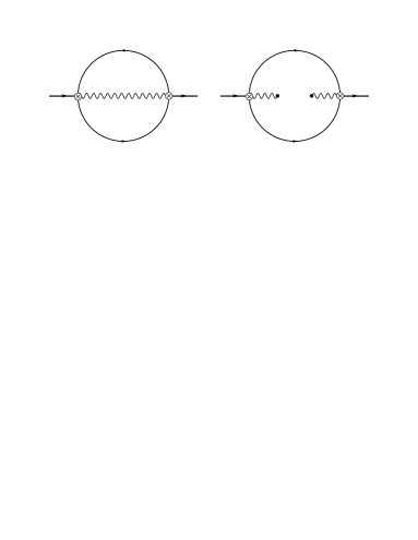
Figure 1: Feynman diagram for the leading-order perturbative and $\langle\alpha\,G^{2}\rangle$ contributions to $\Pi_{\rm V}$. The current is represented by the $\otimes$ symbol.

For brevity only imaginary parts of the perturbative and $\langle\alpha\,G^{2}\rangle$ contributions are given; the full expressions may be found in Ref [7]. We find

$$\begin{split}{\rm Im}\Pi_{\rm V}^{\rm pert}(q^{2})=&\frac{\alpha m^{6}}{180\pi^{2}z^{2}}\Biggl{[}\left(15-35z-22z^{2}-216z^{3}\right.\\ &\left.+48z^{4}\right)\sqrt{z-1}\sqrt{z}+15\left(1-3z+16z^{3}\right)\\ &\times\Biggl{.}\log\left[\sqrt{z-1}+\!\sqrt{z}\right]\Biggr{]}\,,\end{split}$$ (4)

$$\begin{split}{\rm Im}\Pi^{\rm GG}_{\rm V}(q^{2})&=-\frac{m^{2}\langle\alpha G^{2}\rangle}{18}\left(1+2z\right)\frac{\sqrt{z-1}}{\sqrt{z}}\,,\\ &z=\frac{q^{2}}{4m^{2}}\,,\quad z>1\,.\end{split}$$ (5)

Expressions (4) and (5) are in complete agreement with the corresponding integral representations given in [12, 13].

The dimension-six gluon condensate $\langle g^{3}G^{3}\rangle=\langle g^{3}f_{abc}G^{a}_{\mu\nu}G^{b}_{\nu\alpha}G^{c}_{\alpha\mu}\rangle$ contributions are now determined. These were not calculated in Refs. [12, 13], and are represented by the diagrams in Fig. 2. The full expression for these contributions is

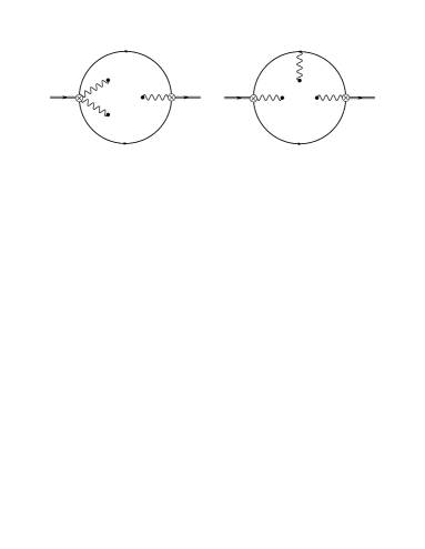
Figure 2: Feynman diagram for the leading-order $\langle g^{3}G^{3}\rangle$ contribution to $\Pi_{\rm V}$. Additional diagrams related by symmetry are not shown.

$$\begin{split}\Pi_{\rm V}^{\rm GGG}(q^{2})=&\frac{\langle g^{3}G^{3}\rangle}{1152\pi^{2}}\Biggl{[}\frac{3(17z-9)}{z-1}-\frac{3(17-46z+27z^{2})}{(z-1)^{2}}\Biggr{.}\\ &+\left(\frac{2z(2-9z+6z^{2})}{(z-1)^{2}}-\frac{4z\left(3z-1\right)}{z-1}\right)\\ &\Biggl{.}\times\,\phantom{}_{2}F_{1}\left(1,1;5/2;z\right)\Biggr{]}\,.\end{split}$$ (6)

The imaginary part of (6) is

$$\begin{split}{\rm Im}\Pi_{\rm V}^{\rm GGG}(q^{2})=&\frac{\langle g^{3}G^{3}\rangle}{384\pi}\frac{\sqrt{z-1}}{\sqrt{z}}\left[\frac{2(1-3z)}{z-1}\right.\\ &\left.+\frac{(2-9z+6z^{2})}{(z-1)^{2}}\right]\,,\quad z>1\,,\end{split}$$ (7)

which is singular at $z=1$. This poses a problem since the sum-rules will involve integrating (7) from $z=1$. Below it will be shown how this difficulty can be overcome.

We now formulate the QCD Laplace sum-rules [17, 18]. Using a resonance plus continuum model for the hadronic spectral function

$$\rho(t)=\rho^{\rm had}(t)+\theta(t-s_{0})\rm{Im}\Pi^{QCD}(t)\,,$$ (8)

the Laplace sum-rules are given by

$${\cal L}_{k}^{\rm QCD}\left(\tau,s_{0}\right)=\frac{1}{\pi}\int_{t_{0}}^{\infty}t^{k}\exp\left[-t\tau\right]\rho^{\rm had}(t)\;dt\,,$$ (9)

where $t_{0}$ is the hadronic threshold. The quantity on the left hand side of (9) is given by

$$\begin{split}{\cal L}_{k}^{\rm QCD}\left(\tau,s_{0}\right)=&\frac{1}{\tau}\hat{B}\left[\left(-1\right)^{k}Q^{2k}\Pi_{\rm V}\left(Q^{2}\right)\right]\\ &-\frac{1}{\pi}\int_{s_{0}}^{\infty}t^{k}\exp\left[-t\tau\right]{\rm Im}\Pi_{\rm V}(t)\;dt\,,\end{split}$$ (10)

where $Q^{2}=-q^{2}$ and $s_{0}$ is the continuum threshold. $\hat{B}$ is the Borel transform, which is closely related to the inverse Laplace transform [19]. The singular terms in (6) that are irrelevant for (7) are, however, relevant for the inverse Laplace transform. It is the inclusion of these terms that allows the integration of (7) from $z=1$ to be defined as a limiting procedure. Thus the imaginary part (7) is insufficient to formulate the sum-rules for $1^{++}$ hybrids, as found for $0^{-+}$ hybrids [16].

From the results for the leading order perturbative (4), $\langle\alpha G^{2}\rangle$ (5), $\langle g^{3}G^{3}\rangle$ (6) and (7) contributions, we find

$$\begin{split}{\cal L}_{0}^{\rm QCD}\left(\tau,s_{0}\right)=&\frac{4m^{2}}{\pi}\Biggl{[}\int_{1}^{s_{0}/4m^{2}}\left[{\rm Im}\Pi_{\rm V}^{\rm pert}\left(4m^{2}x\right)\right.\Biggr{.}\\ &\left.+{\rm Im}\Pi_{\rm V}^{\rm GG}\left(4m^{2}x\right)\right]\exp{\left(-4m^{2}\tau x\right)\,dx}\\ &+\lim_{\eta\to 0^{+}}\left(\int_{1+\eta}^{s_{0}/4m^{2}}{\rm Im}\Pi_{\rm V}^{\rm GGG}(4m^{2}x)\right.\\ &\times\exp{\left(-4m^{2}\tau x\right)\,dx}\\ &+\left.\Biggl{.}\frac{4m^{2}\langle g^{3}G^{3}\rangle}{192\pi^{2}\sqrt{\eta}}\exp{(-4m^{2}\tau)}\right)\Biggr{]}\,,\end{split}$$ (11)

$${\cal L}_{1}^{\rm QCD}\left(\tau,s_{0}\right)=-\frac{\partial}{\partial\tau}{\cal L}_{0}^{\rm QCD}\left(\tau,s_{0}\right)\,.$$ (12)

The mass and coupling are functions of the renormalization scale $\mu$ in the $\overline{\rm MS}$-scheme. After evaluating the $\tau$ derivative in (12), renormalization group improvement may be implemented by setting $\mu=1/\sqrt{\tau}$ [20].

3 Analysis: Mass Predictions for Axial Vector Heavy Quark Hybrids

To make mass predictions for axial vector heavy quark hybrids we utilize a single narrow resonance model

$$\frac{1}{\pi}\rho^{\rm had}(t)=f^{2}\delta\left(t-M^{2}\right)\,.$$ (13)

Inserting (13) in (9) gives

$${\cal L}_{k}^{\rm QCD}\left(\tau,s_{0}\right)=f^{2}M^{2k}\exp{\left(-M^{2}\tau\right)}\,,$$ (14)

which can be used to calculate the ground state mass $M$ via the ratio

$$M^{2}=\frac{{\cal L}_{1}^{\rm QCD}\left(\tau,s_{0}\right)}{{\cal L}_{0}^{\rm QCD}\left(\tau,s_{0}\right)}\,.$$ (15)

Before using (15) to calculate the mass, the QCD input parameters must be specified. For the charmonium and bottomonium hybrid analyses we use one-loop $\overline{{\rm MS}}$ expressions for the coupling and quark masses:

$$\begin{split}&\alpha(\mu)=\frac{\alpha\left(M_{\tau}\right)}{1+\frac{25\alpha\left(M_{\tau}\right)}{12\pi}\log{\left(\frac{\mu^{2}}{M_{\tau}^{2}}\right)}}\,,\;m_{c}(\mu)=\overline{m}_{c}\left(\frac{\alpha(\mu)}{\alpha\left(\overline{m}_{c}\right)}\right)^{\frac{12}{25}}\,;\\ &\alpha(\mu)=\frac{\alpha\left(M_{Z}\right)}{1+\frac{23\alpha\left(M_{Z}\right)}{12\pi}\log{\left(\frac{\mu^{2}}{M_{Z}^{2}}\right)}}\,,\;m_{b}(\mu)=\overline{m}_{b}\left(\frac{\alpha(\mu)}{\alpha\left(\overline{m}_{b}\right)}\right)^{\frac{12}{23}}\,.\end{split}$$ (16)

The numerical values of the QCD parameters are given in Table 1.

$\alpha\left(M_{\tau}\right)$	$0.33$
$\overline{m}_{c}$	$\left(1.28\pm 0.02\right){\rm GeV}$
$\alpha\left(M_{Z}\right)$	$0.118$
$\overline{m}_{b}$	$\left(4.17\pm 0.02\right){\rm GeV}$
$\langle\alpha\,G^{2}\rangle$	$\left(7.5\pm 2.0\right)\times 10^{-2}{\rm GeV}^{4}$
$\langle g^{3}G^{3}\rangle$	$\left(8.2\pm 1.0\right){\rm GeV^{2}}\langle\alpha\,G^{2}\rangle$

Table 1: QCD parameters. The quark masses, $M_{\tau}$ and $M_{Z}$ are taken from Ref. [21]. The values of $\alpha\left(M_{\tau}\right)$ and $\alpha\left(M_{Z}\right)$ are from Ref. [22]. Numerical values of the condensates are taken from Ref. [23].

The sum-rule window is determined following Ref. [17] by requiring that contributions from the continuum are less than 30% of total and non-perturbative contributions are less than 15% of total. These criteria are then used to constrain the Borel parameter $\tau$. This leads to the sum-rule windows of $5.3\,{\rm GeV^{2}}<1/\tau<7.3\,{\rm GeV^{2}}$ for the charmonium hybrid and $7.8\,{\rm GeV^{2}}<1/\tau<25.0\,{\rm GeV^{2}}$ for the bottomonium hybrid.

The continuum threshold $s_{0}$ is optimized by first determining the smallest value of $s_{0}$ for which the ratio (15) stabilizes (exhibits a minimum) within the respective sum-rule windows. Then the optimal value is fixed by the $s_{0}$ which has the best fit to a constant within the sum-rule window. The mass prediction (15) is shown for hybrid charmonium in Fig. 3 and for hybrid bottomonium in Fig. 4.

Figure 3: The ratio ${\cal L}_{1}^{\rm QCD}\left(\tau,s_{0}\right)/{\cal L}_{0}^{\rm QCD}\left(\tau,s_{0}\right)$ for hybrid charmonium is shown as a function of the Borel scale $1/\tau$ for the optimized value $s_{0}=33\,{\rm GeV^{2}}$ (solid curve). The ratio is also shown for $s_{0}=38\,{\rm GeV^{2}}$ (upper dotted curve), $s_{0}=28\,{\rm GeV^{2}}$ (lower dotted curve) and $s_{0}\to\infty$ (uppermost dashed curve). Central values of the QCD parameters have been used.

Figure 4: The ratio ${\cal L}_{1}^{\rm QCD}\left(\tau,s_{0}\right)/{\cal L}_{0}^{\rm QCD}\left(\tau,s_{0}\right)$ for hybrid bottomonium is shown as a function of the Borel scale $1/\tau$ for the optimized value $s_{0}=150\,{\rm GeV^{2}}$ (solid curve). For comparison the ratio is also shown for $s_{0}=170\,{\rm GeV^{2}}$ (upper dotted curve), $s_{0}=130\,{\rm GeV^{2}}$ (lower dotted curve) and $s_{0}\to\infty$ (uppermost dashed curve). Central values of the QCD parameters have been used.

We predict the masses of axial vector charmonium and bottomonium hybrids to be $5.13\pm 0.25\,{\rm GeV}$ and $11.32\pm 0.32\,{\rm GeV}$, respectively. The uncertainties are due to the QCD parameter uncertainties given in Table 1 and are dominated by variations in $\langle\alpha\,G^{2}\rangle$. This is in contrast to the pseudoscalar where variations in $\langle g^{3}G^{3}\rangle$ dominate [16]. These predictions for axial vector heavy quark hybrids are in agreement with those of Refs. [13, 14], suggesting that the effects of $\langle g^{3}G^{3}\rangle$ are less important for the $1^{++}$ channel than for the $1^{--}$ and $0^{-+}$ channels.

4 Conclusions

In Ref. [7] we have studied $J^{PC}=1^{++}$ heavy quark hybrids using QCD sum-rules. For the first time we have calculated the contributions from $\langle g^{3}G^{3}\rangle$, which were found to be important for the $1^{--}$ [15] and $0^{-+}$ [16] channels. We find that $\langle g^{3}G^{3}\rangle$ has less effect on the $1^{++}$ channel, resulting in mass predictions of $5.13\pm 0.25\,{\rm GeV}$ for hybrid charmonium and $11.32\pm 0.32\,{\rm GeV}$ for hybrid bottomonium, in agreement with the range of predictions given in Refs. [13, 14].

The X(3872) has possible $J^{PC}$ assignments of $1^{++}$ or $2^{-+}$ [24, 25], but $1^{++}$ is strongly favoured [26]. In Ref. [27] it was suggested that the X(3872) is a hybrid, but this interpretation has been largely ruled out since the flux-tube model [8] and lattice QCD [9, 10, 11] predict that the lightest charmonium hybrids have masses significantly greater than that of the X(3872). If it is shown to have $J^{PC}=1^{++}$, our mass prediction of $5.13\,\rm{GeV}$ is in agreement with the results of other theoretical approaches that disfavour a charmonium hybrid interpretation of the X(3872).

In Ref. [11] it is suggested that $0^{-+}$ and $1^{--}$ are members of a ground state charmonium hybrid multiplet, while $1^{++}$ is a member of a multiplet of excited charmonium hybrids. The present result and those of Refs. [15, 16] seem to be in qualitative agreement with this multiplet structure, although the mass splittings are significantly larger than those of Ref. [11]. Future work to update remaining unstable sum-rule channels in Refs. [12, 13, 14] to include the effects of $\langle g^{3}G^{3}\rangle$ would clarify the QCD sum-rule predictions for the spectrum of charmonium hybrids.

Acknowledgements: We are grateful for financial support from the Natural Sciences and Engineering Research Council of Canada (NSERC).

References

[1]
S. Eidelman, B. K. Heltsley, J. J. Hernandez-Rey, S. Navas and C. Patrignani,
arXiv:1205.4189 [hep-ex].
[2]
S. L. Olsen,
Nucl. Phys. A 827 (2009) 53C.
[3]
S. L. Olsen,
arXiv:0909.2713 [hep-ex].
[4]
S. Godfrey and S. L. Olsen,
Ann. Rev. Nucl. Part. Sci. 58 (2008) 51.
[5]
G. V. Pakhlova,
arXiv:0810.4114 [hep-ex].
[6]
F. E. Close,
eConf C 070512 (2007) 020.
[7]
D. Harnett, R. T. Kleiv, T. G. Steele and H. -Y. Jin,
arXiv:1206.6776 [hep-ph].
[8]
T. Barnes, F. E. Close and E. S. Swanson,
Phys. Rev. D 52 (1995) 5242.
[9]
S. Perantonis and C. Michael,
Nucl. Phys. B 347 (1990) 854.
[10]
L. Liu, S. M. Ryan, M. Peardon, G. Moir and P. Vilaseca,
arXiv:1112.1358 [hep-lat].
[11]
L. Liu, G. Moir, M. Peardon, S. M. Ryan, C. E. Thomas, P. Vilaseca, J. J. Dudek and R. G. Edwards et al.,
JHEP 1207 (2012) 126.
[12]
J. Govaerts, L. J. Reinders and J. Weyers,
Nucl. Phys. B 262 (1985) 575.
[13]
J. Govaerts, L. J. Reinders, H. R. Rubinstein and J. Weyers,
Nucl. Phys. B 258 (1985) 215.
[14]
J. Govaerts, L. J. Reinders, P. Francken, X. Gonze and J. Weyers,
Nucl. Phys. B 284 (1987) 674.
[15]
C. -F. Qiao, L. Tang, G. Hao and X. -Q. Li,
J. Phys. G 39 (2012) 015005.
[16]
R. Berg, D. Harnett, R. T. Kleiv and T. G. Steele, Phys. Rev. D., to appear
[arXiv:1204.0049 [hep-ph]].
[17]
M. A. Shifman, A. I. Vainshtein and V. I. Zakharov,
Nucl. Phys. B 147 (1979) 385.
[18]
M. A. Shifman, A. I. Vainshtein and V. I. Zakharov,
Nucl. Phys. B 147 (1979) 448.
[19]
R. A. Bertlmann, G. Launer and E. de Rafael,
Nucl. Phys. B 250 (1985) 61.
[20]
S. Narison and E. de Rafael,
Phys. Lett. B 103 (1981) 57.
[21] Particle Data Group (K. Nakamura et. al), J. Phys. G 37 (2010) 075021.
[22]
S. Bethke,
Eur. Phys. J. C 64 (2009) 689.
[23]
S. Narison,
Phys. Lett. B 693 (2010) 559
[Erratum-ibid. 705 (2011) 544].
[24]
A. Abulencia et al. [CDF Collaboration],
Phys. Rev. Lett. 98 (2007) 132002.
[25]
K. Abe et al. [Belle Collaboration],
hep-ex/0505038.
[26]
N. Brambilla, S. Eidelman, B. K. Heltsley, R. Vogt, G. T. Bodwin, E. Eichten, A. D. Frawley and A. B. Meyer et al.,
Eur. Phys. J. C 71 (2011) 1534.