A Detailed Far-Ultraviolet Spectral Atlas of O-Type Stars

Abstract

In this paper we present a spectral atlas covering the wavelength interval 930–1188  Å for O2–O9.5 stars using Far Ultraviolet Spectroscopic Explorer archival data. The stars selected for the atlas were drawn from three populations: Galactic main sequence (class III-V) stars, supergiants, and main sequence stars in the Magellanic Clouds, which have low metallicities. For each of these stars we have prepared FITS files comprised of pairs of merged spectra for user access via the Multi-Mission Archives at Space Telescope. We chose spectra from the first population with spectral types O4, O5, O6, O7, O8, and O9.5 and used them to compile tables and figures with identifications of all possible atmospheric and ISM lines in the region 949-1188  Å.  Our identified line totals for these six representative spectra are 821 (500), 992 (663), 1077 (749), 1178 (847), 1359 (1001), and 1798 (1392) lines, respectively, where the numbers in parentheses are the totals of lines formed in the atmospheres, according to spectral synthesis models. The total number of unique atmospheric identifications for the six main sequence O star template spectra is 1792, whereas the number of atmospheric lines in common to these spectra is 300. The number of identified lines decreases toward earlier types (increasing effective temperature), while the percentages of “missed” features (lines not predicted from our spectral syntheses) drops from a high of 8% at type B0.2, from our recently published B star far-UV atlas, to 1–3% for type O spectra. The percentages of overpredicted lines are similar, despite their being much higher for B star spectra. We discuss the statistics of line populations among the various elemental ionization states. Also, as an aid to users we list those isolated lines that can be used to determine stellar temperatures and the presence of possible chemical anomalies. Finally, we have prepared FITS files giving pairs of merged spectra for stars in our population sequences for access via the Multi-Mission Archives at Space Telescope.

1. Introduction

High dispersion spectroscopy provides windows into the past and current physical processes in massive O stars as clear as for stars anywhere on the H-R Diagram. Individual O stars can be found in different stages of evolution because of their short lifetimes and unique spectral signatures that advertise these stages. Indeed, many of them evolve to SN Ib and SN Ic supernovae by first becoming Luminous Blue Variables and/or Wolf-Rayet stars, which are easily identifiable by their light curves or broad spectral emission features. Likewise, O stars in close binaries are readily discovered from emission in optical and UV lines excited by interacting winds. Because the incidence of lines in O star spectra and continuum flux both peak in the far-ultraviolet wavelength region, the use of space-borne instrumentation is critical to fully understanding their atmospheres and radiative processes. Although observations with the Far Ultraviolet Spectroscopic Explorer satellite (FUSE) were terminated in 2007, the FUSE archive now offers a large sample of stellar spectra having identical wavelength coverages provided by homogeneous data processing. In particular, FUSE-accessible O stars reside not only within the solar neighborhood in the Galaxy but also in the more distant Magellanic Clouds. Because their lifetimes are brief, O stars provide an invaluable record of the recent chemical composition and angular momentum histories in the solar neighborhood and the return of much of their nuclear-processed matter to the Interstellar Medium (ISM).

Astronomers have historically been quick to capitalize on uniformly reprocessed data held in archives following the close of UV spectroscopic mission. The availability of these archives has allowed the construction of a number of fine spectral atlases recorded by the Copernicus and the International Ultraviolet Explorer ( IUE) satellites. Important examples of these compilations for the middle-UV spectral range are the Copernicus atlas of $\tau$ Sco (Rogerson et al. 1978) and IUE pictorial atlases of O and B stars (Walborn, Nichols-Bohlin, & Panek 1985, Rountree & Sonneborn 1993, Walborn, Parker, & Nichols 1995). Pellerin et al. (2002) inaugurated a second group of digitized far-UV (FUSE) atlases consisting of representative spectra of O and early-B type, luminosity class I-V stars in the Galaxy and Magellanic Clouds. These atlases have been supplemented by figures constructed by N. Walborn for the Gray & Corbally (2009) monograph on stellar spectral classification that show the changes of primary spectral features in the far-/middle-UV with luminosity class in main sequence O stars.

Such atlases have been effective in showcasing the general trends of the strong photospheric lines and the so-called “UV resonance wind” lines with effective temperature T_eff and luminosity class. For example, a reconnaissance of the O-star (Pellerin et. al) atlas shows how far-UV spectra of most O stars are strongly mutilated by interstellar lines, particularly below 1100  Å. The photospheric component of these spectra is dominated by the confluence of high series Lyman lines, Ly$\beta$–Ly$\theta$ down to the blue limit of the FUSE instrument at 920  Å.  The strongest metallic feature formed substantially in the photosphere is generally the C III line complex at 1174–1176  Å. This multiplet arises from an excitation of the lower atomic levels at an excitation $\chi$_exc = 9 eV.  In supergiant O stars radiative winds can cause this complex to develop into a broad P Cygni profile. Other strong features are resonance lines of C III (977  Å), N III (991  Å), O VI (1031  Å,  1037  Å), Si IV (1128  Å), S IV (1062  Å,  1072  Å,  1073  Å,  1098–1100  Å), P IV (950  Å), and P V (1117  Å,  1128  Å). Spectral lines of O stars suffer doppler broadening, and this serves to wash out isolated weak metallic lines that would otherwise be resolved in high dispersion spectra. However, as detailed below, the far-UV spectra have the saving grace that, except for the liberally distributed ISM lines, the photospheric lines tend to be more widely spaced and to blend less with one another than in the middle-UV wavelengths.

The Pellerin et al. atlas and Barnstedt et al. (2000) have displayed valuable detailed information about the presence of molecular H₂ features formed in the ISM. From the point of view of stellar atmosphere investigators, these features contaminate many of the far-UV lines formed in the atmospheres of most Galactic stars. The Pellerin et al. atlas was closely followed by a second spectral atlas of OB stars in the two Magellanic Clouds (Walborn et al. 2002). This work concentrated on the behavior of wind lines with respect to metallicity as well as effective temperature and luminosity. In addition, Blair et al. (2009) published a compendium of FUSE spectra of hot stars in the Magellanic Clouds. This atlas focused on the identification of far-UV resonance lines formed in the ISM, including those found at multiple velocities.

The first far-UV high-dispersion spectral coverage published for a B star was the Copernicus atlas of $\tau$ Scorpii (B0.2 V; Walborn 1971) by Rogerson & Upson (1978). Rogerson & Ewell (1985; “RE”) published a detailed tabulation of atmospheric and ISM lines identified in this atlas. The RE work was undertaken at a time when spectral synthesis tools were not commonly available, and when only a relative handful of experienced spectroscopists who were also specialists in atomic physics could make reliable line identifications. Even so, in the absence of commonly available synthesis programs at that time, it was difficult to make wholesale line identifications without some errors. This situation has changed dramatically in the intervening years with the development of spectral line synthesis tools that make use of extensive atomic line libraries.

Inspired by the Copernicus atlas, Smith (2010; hereafter “Paper 1”) constructed a far-UV spectral atlas for B stars using spectra from FUSE  IUE, and the Space Telescope Imaging Spectrograph (STIS) over the (vacuum) wavelength range 930–1225 Å.  In making this atlas we set an arbitrary short wavelength limit of 930  Å because, other than for a few blended Lyman lines, no useful information about the photospheric spectrum could be obtained below this wavelength. We chose the red limit by including spectra from the HST/STIS and/or IUE cameras in order to cover the Lyman $\alpha$ feature and other important lines in its vicinity. The B star atlas addressed its first goal of fulfilling the need for the identification of all possible visible lines in the “template” spectra of three representative main sequence B0.2 V, B2 V, and B8 V stars. These identifications were made by using published atomic line libraries that predict occurrences of lines from spectral synthesis models. This atlas also recorded “misses,” i.e., the wavelengths of observed lines that could not be predicted from our line syntheses. The rotational velocities of stars selected for the atlas are relatively low in order to resolve as many neighboring photospheric lines as possible. Therefore, we referred to this work as a “detailed spectral atlas.” The second goal of this atlas was to provide uniform spectral data products to the astronomical community through the wavelength range just described.

The numbers of lines identified for the three template spectra in Paper 1 were 2288 (2004), 1612 (1465), and 2469 (2260) lines, respectively. Here the values given in parentheses are the number of lines found within almost the full wavelength range covered by the FUSE  949–1188  Å.  Of these totals only small percentages (8%, 2%, and 2%, respectively) of photospheric lines could not be identified, which is to say that the oscillator strengths (log $gf$’s) for these lines are at best poorly determined and are thus not included in our line library. The B star atlas results were published more fully in the electronic edition, The spectral data files and all other products were made available for public download as one of MAST’s “High Level Science Product” (HLSP) area (http://archive.stsci.edu/prepds/fuvbstars/).

This paper presents a similar spectral atlas for O stars. The atlas is organized in much the same way as the B star atlas. However, one important difference is that whereas the blue wavelength limit we chose, 930 Å, is the same as for the B star atlas, the red one is set by the FUSE spectral coverage, again, $\approx$1188 Å. In particular, we found for the present atlas that it was not easy to again include the 1188–1225 Å region that was previously surveyed in the B star atlas because of the paucity of O stars observed systematically in this spectral region.

Our presentation is organized as follows. The selection of spectra and the methodology for data handling, including the creation of FITS spectra for all stars in our sample, as well as for the line identification in six exemplars, are described in $\S$2. In $\S$3 we display portions of the atlas and give a detailed list of several thousand identifications as well as a list of “clean” lines across much of the O-star domain. In $\S$4 we give relevant statistics from our identifications for the six O4 V, O5 V, O6.5 V, O7 III, O8 V, and O9.5 III exemplars we call our O star spectral templates. We also comment in detail on a number of possible spectral markers for physical conditions (mainly effective temperatures) in these stars’ atmospheres, all of which are assumed to be in hydrostatic equilibrium.

2. Preparation of the Atlas

2.1. Atlas star selection

The selection of stars for our atlas was based on a number of criteria. These included high signal-to-noise ratios (SNR), absence (so far as is known) of double-lined binary signatures, low to moderate rotational broadening ($v\,sin\,i$ $\mathrel{\hbox{\hbox to0.0pt{\hbox{\lower 4.0pt\hbox{$\sim$}}\hss}\hbox{$<$}}}$ 100 km s^-1), and far-UV extinction ($E(B-V)<$ 0.4) from the ISM. An additional criterion was that their surface iron group metallicities should be close to those of most other Galactic young massive stars in the solar neighborhood. We also wanted to augment the scope of atlas by including supergiants, even though their lines are usually affected by rotational and atmospheric doppler broadening mechanisms. While all these criteria are desirable for a spectral atlas of massive hot stars in the local region of the Galaxy, they can conflict with one another at times. A second issue affecting our our selections is that those stars with solar-like compositions are strongly confined to the Galactic plane and suffer extensive contamination by molecular H₂ and atomic ISM features as well as attenuation from ISM dust. This absorption peaks in the far-UV region. To include representative O stars beyond the plane that exhibit smaller amounts of far-UV absorption, one is generally obliged to find them in one of the Magellanic Clouds, and these stars have low metallicities. Altogether, we included parallel sequences of main sequence (luminosity class III-V) stars observed at high galactic latitudes (members of the Magellanic Clouds) as well as a third sequence of supergiants (class I–II).

A survey of the O star data in the entire MAST/FUSE archive demonstrated that we could not fill a table of representative stars across the O domain using all these sometimes conflicting criteria. In particular, we could not find spectra in the archive of stars having spectral types of O2 and O3 and supergiant luminosity classes. Otherwise, we were able to find three stars per spectral type over the range O4–O9.5, giving us a total of 25 stars. These stars, their spectral types, and $v\,sin\,i$ values, and references for these values are listed in Table 1. We took most of these spectral types from the compilations of Howarth et al. (1997; “H97”) and Penny & Gies (2009; “PG09”). We have grouped names of three stars for spectral type (excepting O2 and O3) in order of the three stellar populations listed just above.

Stars marked by asterisks in the table represent the six main sequence template stars referred to above. For our line identification tables for six main sequence stars we assign “star code” values of 1–6 to those stars in our line identification tables. In our system the value 1 corresponds to subtype O9 5, 2 to O8 (omitting O9), and so on, until the value 6 is applied to O4. Note in addition that we were not able to find high quality spectra of examples of O2 and O3 supergiants.

2.2. Data properties and handling

2.2.1 Conditioning of FUSE spectra

During its eight year lifetime the FUSE spacecraft was operated with four independent spectrographs/cameras. As described in the FUSE Archival Instrument Handbook (Kaiser & Kruk 2009), light collected from each of the telescopes illuminated a holographic diffraction grating/camera mounted on a Rowland circle spectrograph. LiF and SiC coated camera mirrors focused the dispersed light on two far-UV microchannel plate detectors. Table 2 lists in italics the (vacuum) wavelength coverage of each of the FUSE detector segments. As noted above, nearly complete far-UV coverage of the spectrum was provided by two nearly identical “Sides” 1 and 2 of the instrument. Each of these Sides included two pairs of LiF and SiC detectors. The parenthesized wavelengths intervals in the table give the regions for each Side/detector combination. Coverage of each wavelength was provided by each of the two Sides, with two exceptions: (1) data for the wavelength interval 1090–1094.5  Å were recorded only from Side 2 detectors, and (2) data for 1015–1075  Å were recorded by all four detectors. The spectral resolution (full width half maxima) of FUSE spectra is 15-20 km s^-1, i.e., 0.05–0.07  Å, though this varies slightly from one detector segment to another. Spectral fluxes were sampled by the pipeline processing system at uniform intervals of 0.013  Å , and we maintained this spacing in our products.

The conditioning steps needed to produce continuous spectra from FUSE archival data are somewhat complex. First, the wavelength calibrations for FUSE spectra are known to undergo excursions from a linear dispersion of up to $\pm{0.03}$  Å over intervals as short as 5  Ångstroms. These excursions are largely due to electron repulsion in the detector that distort the positions of recorded photoelectrons in the detector $x$ and $y$ axes. The effects are typically not robust with time and therefore cannot be modeled or compensated for reliably. In addition, small wavelength shifts due to positioning and wandering of the star image in the science apertures are the norm. Since most of our spectra were obtained with multiple exposures, the first step in correcting them was to cross-correlate them inter alia to introduce subpixel shifts to the system of the first observations. The shifted spectra were manually inspected to insure that this step was performed accurately. We then coadded the spectra according to the pipeline-generated errors for the individual exposures. To remove any residual offset shifts and local departures from the mean dispersion, we wrote a program in the Interactive Data Language to view and match the observed features of the Side 1 and Side 2 spectra with a comb spectrum of H₂ features provided by the online “H2ools” tool (McCandliss 2003). The features in H2ools matched the computed Lyman and Werner transitions from a single rotational state of the zeroth or occasionally first vibrational level to the ground state of molecular H₂ lines. It is important to point out one key difference between ISM and photospheric line identifications: whereas the photospheric lines are based on predictions from the line synthesis spectra for an assumed T_eff of a spectral type, all ISM identifications are based on their visibility in the template spectra. This could mean, for example, that a given H₂ feature may not be found in a particular template spectrum if the column density toward the star referred to is smaller than toward other stars.

To reference the absolute wavelength system from the H₂ features we had to rely on estimates of the locations of strong unblended photospheric lines relative to nearby H₂ features. The doppler shifts of our Galactic stars are typically within $\pm{0.05}$ Å. Exceptions to this statement are for our O8 V line identification star HD 66788 and the O9 Ib-II star HD 207198. The HD 66788 spectrum is an unusual case because it relies on a single FUSE exposure. The spectrum showed a wavelength shift of +0.6  Å ($\approx$85 km s^-1) from the Galactic system set by the H₂ lines. The dataset for HD 207198, which is known to be in a spectroscopic binary, is comprised of five exposures over two epochs. Their shifts are the same for each of two common epochs, but the archived spectra in one group are shifted 4 pixels from the spectra of the other group. When referenced to the first epoch, the averaged spectrum exhibits an additional shift of +0.2  Å with respect to the H₂ scale. Thus, both stars appear to be primaries of binary systems. However, we could not discern line components of a secondary star in the spectrum. The pipeline spectra of all the Magellanic (AZ and Sk) objects are shifted from the Galactic H₂ wavelength system by +0.6  Å, except for the O8 V star D301-NW8, which is shifted by +1.2  Å. The spectral shifts from the nine observations suggest that this object is the primary of a second undiscovered binary system in our star list. Such large wavelength shifts are handy to have in our sample because they help to separate contributions of overlapping features formed in the photosphere and ISM. We have also made judicious use of this advantage by using the O8 template to arbitrate between identifications in other spectra that are unshifted from the rest (ISM H₂) frame.

A final complication in FUSE spectra was the occurrence of optical vignetting across the detector fields called “worms.” These cause recognizable flux depressions across certain detector segments, especially for the LiF 1B segment in the region 1130  Å to 1160  Å (see Chapter 4 of Kaiser & Kruk 2009). We addressed this feature by passing a high order filter having the same degree over the 1B and 2A segment fluxes and then interpolating to the original pixel scale. The depression in the Side 1B spectrum was mitigated by dividing the smoothed polynomial fit of the 2A spectrum by the similarly smooth fit of the 1B one in the wavelength region affected by the worm. The quotient spectrum was then applied to the original 1B spectrum. A second worm in the LiF Side 1 detector spectrum occurs in the region 997–998  Å. However, this worm was left uncorrected in the plots and spectral data discussed below. In addition to worms, we noticed that occasional drop offs of flux at the ends of segments, e.g., 1087–1088  Å for SiC-B Side 2. These occurrences appeared over too short a wavelength span to correct. Otherwise, because several instrumental idiosyncracies appear in FUSE detector Sides 1 and 2 spectra, most researchers have learned to work with the segments of these two sides separately and to compare them in the end as if they were independent observations. We have done the same in preparing our atlas by merging the four segments of the two sides to form two long spectra, with break points given in Table 2. Thus, the last step in establishing the wavelength calibration was to correct the spectra for the radial velocity shifts discussed above and to interpolate them to the initial grid from the pipeline system, that is, starting at 920.0  Å and incrementing by 0.013  Å to about 1188.4  Å. The spectra for the 25 stars in this atlas are given for the two independent detector sides as separate extensions in our products, which are Flexible Image Transport System (FITS) files, formatted as binary numbers.

2.3. Tools for line identifications

2.3.1 Six template spectra

We expect the primary use of our atlas will come from the consultation of line identification tables and annotated plots discussed below. It is unnecessary and time-consuming to attempt to identify lines according for each of the 25 stars given in FITS format. Our philosophy is to identify all lines that can be predicted in the far-UV spectrum in increments of effective temperature of $\approx$2 kK up to T_eff = 42 kK. (Our model atmospheres line synthesis program discussed below operates on models computed with T_eff values in integral kilokelvins.) We chose six template representative spectra of metal-normal O dwarf stars for our line identifications. Our T_eff values in Table 1 are for the most part those that follow the spectral type calibration of Martins, Schaerer, & Hillier (2005, their Table 4). The exception to this practice is that we used T_eff = 34 kK (rather than 35 kK) to the value that Marcolo et al. (2009) determined for our O8 V star, HD 66788. We note also that the value T_eff = 32 kK used for the O9.5 V template spectrum is similarly spaced from the highest value, 30 kK, that we used in Paper 1 for identifications in the “anchor” (Copernicus) spectrum of $\tau$ Sco.

2.3.2 Construction of the line library

To prepare for the identification of lines in our spectral templates using spectral synthesis models, we compiled a line library from three sources: the Kurucz (1993) line library, the Vienna Atomic Line Database (“VALD”; Piskunov et al. 1995, Kupka et al. 1999), and the on-line atomic line database of van Hoof (2006). The Kurucz line library is comprehensive and determined from atomic theory computations. In the far-UV this provides the advantage that the library coverage is not compromised as it otherwise could be by absorptive optical coatings used in laboratory spectrographs. However, even though it continues to provide most of the identifications we used, many of the oscillator strengths (log $gf$s) in this list have become dated. By contrast, the VALD and van Hoof databases are periodically updated. Both also give a recommended log $gf$ value for a line if more than one have been published. The VALD library is supported by an interactive web interface. This access tool allows a user to input on an web form a rough photospheric effective temperature and as well as line depth threshold criterion, in our case 1% line depth. All lines computed with depths larger than the threshold were included in a returned list. We exercised this option and chose parameters T_eff = 35 kK and solar abundances in our requests to VALD of expected detectable lines through our line identification -UV region, 949  Å to 1188  Å. The short limit was set as the starting point of the Copernicus atlas for $\tau$ Sco. We repeated the procedure with T_eff = 45 kK. Our requests to VALD using these two effective temperature resulted in the addition of new lines to our original B star line library. The van Hoof tool is convenient to use both in augmenting the atomic line list and for the spot checking we occasionally had to do to confirm our automated line synthesis results.

The final stage of the line selection was to screen out line duplications that sometimes occur in combining lines from different library sources. We accomplished this by writing a program to run through our list and identify line entries within ${\pm 2}$ m Å  arising from lower excitation levels within ${\pm 0.03}$ eV of the same ion. In these cases lines with the smaller log $gf$ values were culled out. The results from the additions and screenings was that we could import some 2500 new potential line candidates to our atomic line library. With this step completed our library became suitable for synthesis of both O or B type spectra. It is available upon request to the author.

2.3.3 Line synthesis

All our line identifications were based on our just described line library. To summarize the result, all lines in our library have either measured or computed log $gf$ values taken from the above referenced sources. To make line identifications operationally we used a line annotation facility in the spectral line synthesis program SYNSPEC49 of Hubeny, Lanz, and Jeffery (1994). This program can be run interactively to compute and plot spectral fluxes over a specified wavelength range once the user specifies key parameters such as metallicity, stellar effective temperature T_eff, log $g$, and microturbulence. In our models we used log $g$ = 4, $\xi$ = 5 km s^-1, and solar abundances. We executed the manual steps outlined below three times to minimize errors.

We also compared line synthesis results from standard Kurucz (1990) and non-LTE models calculated by TLUSTY described by Lanz & Hubeny (2003), as updated by a “OGA grid” conveyed by T. Lanz to the author. The primary improvement in the new grid was the addition of a number of excited levels of light and iron group ions for non-LTE computations for lines of these ions. The line strengths produced from LTE and non-LTE models typically differed by amounts equivalent to a temperature change of 1,000 K. The spectra computed from the LTE and non-LTE led to nearly identical identifications. In those few cases where differences occurred, we took the identifications from the non-LTE atmospheres models. Also, we erred on the side of reporting a possible identification rather than not doing so. In general the errors in the computed line strengths owe more to to the low precision of the log $gf$’s than to uncertainties in details of line formation in the atmospheres.

2.3.4 Line identification methodology

In this atlas we describe the philosophy and general methodology of producing a list of line identifications predicted by model synthesis programs. Those features observed in the template spectra at wavelengths where no plausible identification can be made are annotated by the symbol of a fictitious element, “UN I” (for “unknown”), in our tables. We refer to these below as “missed” features. Without exception the photospheric spectra of our selected stars exhibit at least moderate broadening. Therefore, unidentified stellar features could be readily differentiated from the narrower atomic and molecular features.

In the far-UV a particular challenge is identifying components of closely spaced individual lines. To differentiate potential partially resolved lines we set a resolution window criterion of ${\pm 80}\,$mÅ.  Lines within this window were considered for identification purposes to be completely blended. Our procedure was to compute spectral line models in small wavelength intervals and to overplot the synthesis and the identifications provided by SYNSPEC on a computer screen. Manual intervention was sometimes required in assembling the identification list for each template spectrum for the following reasons:

1. The log $gf$ values of far-UV lines can be uncertain and occasionally overpredict the line’s observed strength; that is, a line is predicted by SYNSPEC but is not observed. We introduced a “:” symbol in the atlas figures and identification tables in cases where the overprediction exceeded a factor of 30 of the log $gf$ needed to make the predicted line easily visible (i.e., a line depth of $\sim$10%).

2. Closely spaced lines can blend in line syntheses. We chose a blend window of ${\pm 80}$ m Å] to represent lines within a line “group.” In these groups we gave primacy to the dominant (primary) line and listed the secondary lines (members of the common group) in a separate column of our identification table (see Tables 3 and 4). In practice, almost all detectable far-UV lines are at least partially saturated. Thus, lines contributing less than the primary line’s absorption do not contribute much to a line group’s aggregate strength. Unless multiple secondary lines are present within a group, we found that the strengths of ensemble group features are dominated by the contribution from the primary lines.

The construction of our line list proceeded only after putting into place semiautomated error checking procedures. One such procedure was to check the ions and exact wavelengths against those in our line library. Our program reported any errors in this collation, and they were corrected. Nonetheless, we cannot claim that our list of identifications is completely error-free! The influences of some lines may yet have been over- or underestimated. Second, we checked our line identifications with other published abbreviated lists of prominent far-UV lines, including those in the Pellerin et al. (2002) atlas and the far-UV Capella atlas (Young et al. 2001). We noticed minor deviations in quoted wavelength values for several lines, and in a few cases we could not confirm their line identifications because we could not find log $gf$ values in their secondary sources. Third, we checked the major far-UV transitions noted for the light metal elements in the Grotrian diagrams published in the Bashkin & Stoner (1975) compendium. The absence of any significant discrepancies in these comparisons suggests that there are few or no gross or systematic errors in our list. Our experience in constructing two atlases suggests that the greatest source of errors is in incorrectly estimating the relative strengths of photospheric and ISM (especially from atomic species) contributions. Nonetheless, in all we believe our identified and unknown lines form a list of essentially all the visible features that contribute the far-UV absorption lines of Galactic main sequence O4–O9.5 stars.

3. The O star spectral atlas

3.1. The atlas and associated data products

Our O star atlas is different from most other atlases, though it is similar in appearance to our B star atlas. The atlas consists of three core products: (1) extensive line identification lists, (2) a graphical plot of line identifications of the template spectra, and (3) data files containing merged spectra in FITS format for all 25 atlas stars. The FITS files contain the Side 1 and Side 2 spectral data in two extensions. Each extension contains a wavelength, flux, and pipeline-generated flux error vector.

The full line identification tables and line-annotated spectral plots for the six template stars, as well as the spectra in FITS format for all 25 stars (including those drawn from the supergiant and Magellanic Cloud populations), have been placed, coincident with this paper’s publication in MAST’s High Level Science Products (HLSP) web area (http://archive.stsci.edu/prepds/fuvostars/), where the products are further vetted by MAST staff for clarity and ease of access. The full line lists and plots for the six template files are also accessible at this web site. Users can report any errata, which MAST will include as part of the HLSP. In addition, a copy of our compiled line library will be provided upon request to the author. Finally users of the HLSP or the individual FUSE archival data files will find electronic links to this paper held by the NASA Astrophysical Data System (ADS) and, conversely, links at the ADS site to the paper also include links to the FUSE data used herein.

Our detailed line lists for the O9.5–O7 and O6–O4 main sequence template spectra are presented as stubs in Tables 3 and 4 in the paper edition of this work. The full tables are given in the electronic version of this paper in ASCII Comma Separated Value format. Each subpanel lists the spectral type by star code, 1–6. The star code listed applies only to identifications for the table’s spectral subtype and later subtypes. In the next two columns we give the identified wavelength from our line list catalogs and and finally the ion corresponding to the line identification. The two wavelength columns represent either the “primary” or “member” (secondary) of a line group, respectively, such that one of the columns is always unfilled. Here “group” refers once again to lines occurring a common resolution window in which the primary line is located. According to this definition, we found as many as 6 secondary group members associated with a primary line (generally no more than half of which are photospheric lines). In these tables wavelengths of photospheric and ISM lines are given in the same (rest) system.

The rows of Tables 3 and 4 are sorted according to the primary line wavelength of each group and are interleaved among the three template spectra. The electronic edition of this paper gives this as a single monolithic table, with each spectral type subtable separated from the next by a header. Secondary group members follow their associated group primaries, even if the secondary’s wavelength is slightly smaller than the primary’s. This practice insures that lines do not appear in more than in one column for a given star.

As in Paper 1 we list in Table 5 wavelengths of “isolated” (least contaminated) photospheric lines that are “universal” (that is, visible in at least the O5–O8 template spectra) for light elements and some iron-group ions. In particular, note that the lines in these tables may lie further away from H₂ features than our formal ${\pm 0.08}$  Å resolution bin but still may be useless if the latter are pressure broadened. Table 6 gives isolated Fe V lines arising from the Fe⁴⁺ ion, which as we will see is the dominant contributor to photospheric lines for middle-O stars. The electronic edition of this paper presents this table in its full length, listing 135 lines. The Fe⁴⁺ ion continues to contribute lines in the far- and middle-UV to spectral types as late as B0.2 for main sequence stars. The tables also give the range of excitation potentials, in eV, of lines for an ion. The coding system in this table gives the same running star number (“1” for O9.5, “2” for O8, etc.) as for previous tables. A null (blank) value means that a line is not predicted in the spectrum. Blanks occur most commonly in the O4 and O9.5 star columns for low or high excitation ions, respectively.

Figures 1 and 2 depict 3-panel samples of the atlas over the 1070–1077.5  Å wavelength interval for our O9.5, O8, & O7 and O6, O5, & O4 template spectra, respectively. This is the same interval depicted in Fig. 1 of the B star atlas and thus provides continuity for paper edition readers of the line coverage for O and B type stars.

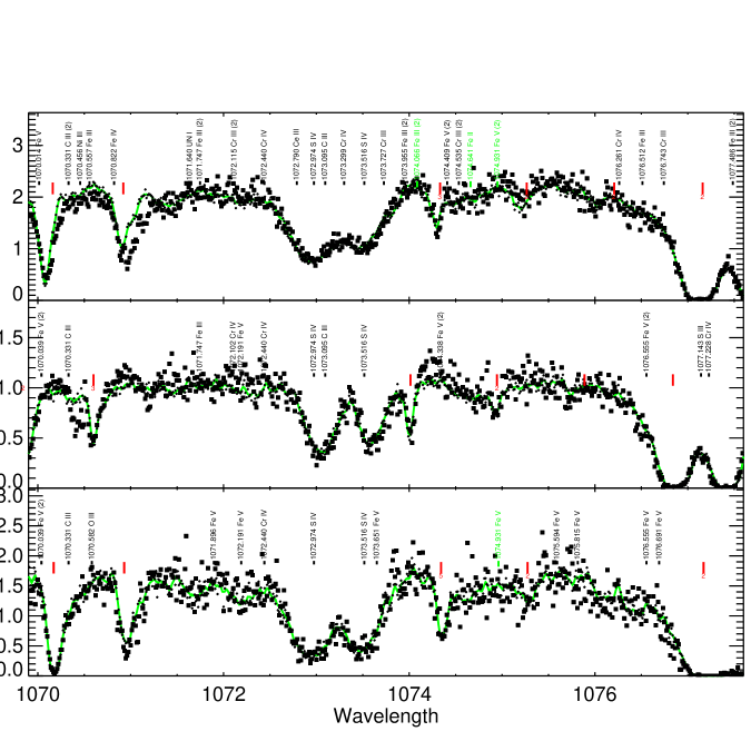
Figure 1.— Spectral atlas and line identifications depicting the wavelength region 1070–1077.5 Å for O9.5, O8, and O7 stars (top to bottom) near the main sequence. The green line represent a filtered FUSE spectrum taken from Side 1 detectors; small squares represent Side 2 data. Line identifications are represented vertically by ion and vacuum wavelength and with colons when they are uncertain. Notations such as “(2)” represent the combined number of primary and secondary lines in a wavelength resolution bin. Annotations also represent atomic ISM lines while thick vertical ticks represent ISM H₂ features; the online plots show these features in green and red, respectively. For the paper version wavelengths of atomic ISM lines in this and the following figure are followed by “+ ISM.” Numbers are associated these too if they are primaries in local wavelength groups. Fluxes units are 10^-11 ergs s^-1 cm^-2 Å^-1.

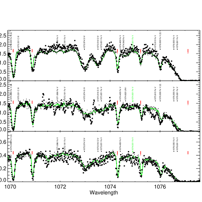
Figure 2.— A continuation of the spectral atlas and line identifications in the wavelength region 1070–1077.5 Å for O6, O5, and O4 stars (top to bottom) near the main sequence. Symbol identifications are the same as in Fig. 1. The ion “UN I” represents an unidentified absorption line not predicted by our atmospheres models. Fluxes are in units of 10^-11 ergs s^-1 cm^-2 Å^-1, except for the O4 star (bottom panel), for which the exponent is -12.

Because the stars have individual random radial velocities with respect to the local Galactic ISM system, we present in the figure the spectral lines and their annotations in their respective velocity systems, according to where the lines are formed. This is to say, in the figures we correct for the stars’ radial velocities such that the photospheric lines appear in our local rest frame whereas all H2 lines carry the reflex of the stellar spectrum’s velocity. Two ramifications of this wavelength difference are, first, that the composition of the mixed star-ISM line groups can differ for our tables and figures. This is because the photospheric wavelengths in the figures are always represented in the laboratory system. Second, the ISM lines in the spectrum with the velocity shifts will be displaced with respect to the positions of the same lines in unshifted spectra shown in another figure panel. The best example of this is the HD 66788 spectrum (Fig. 1), for which as already noted the ISM lines are shifted relatively to photospheric lines by -0.6  Å.  Then, in the middle panel of Fig. 1 the vertical ticks signifying the H₂ lines are displaced to the left by this amount, whereas spectra in the upper and lower panels are unshifted.

4. Discussion

4.1. Line statistics

Even a glance at the Tables 3 and 4 suggests that the density of photospheric lines, e.g., those in the range 949–960.0 Å, decreases towards earlier types. For the same wavelength range the number of lines for the B0.2 template was 81 (Paper 1), and in our tables it is 53 for O9.5 V and 24 for O4 V. Near the long wavelength limit, 1170-1188.5  Å, the corresponding decline in numbers of identifications is as least as dramatic, from B0.2 to O9.5 to O4: 128, 97, and 31, respectively. Another important generalization is that with few exceptions the strongest features in the observed spectra are ISM or hydrogen Lyman lines – that is, nearly all metallic lines are weak. One can get a superficial impression that strong photospheric features appear in far-UV spectra of earlier type stars, but this is due to saturation of wings of strong H₂ features because of longer ISM column lengths to these distant stars. The numbers of all identified lines in our Tables 3 and 4, including ISM ones, total 1798, 1359, 1178, 1077, 992, and 821, for O9.5, O8, O7, O6, O5, and O4, respectively. When we separate out the ISM lines the totals for photospheric lines alone are 1392, 1001, 847, 749, 663, and 500, respectively. The totals are depicted by a thick dotted line in Figure 3. As one proceeds to earlier O spectral types, the downward trend shown by these totals contrasts with the nonmonotonic numbers of lines found along the B spectral sequence in Paper 1. In the comparable far-UV wavelength region those numbers were 2182 (B8), 1398 (B2), and 1991 (B0.2). Not surprisingly, one finds that there is a fair degree of overlap among lines of neighboring spectral subtypes. The total number of unique photospheric identifications is 1792. The number of photospheric lines we identified for all six O spectral types is 300. Note that because our stellar line identifications are based on line synthesis predictions (except for missed features seen in the spectra), our O star statistics are not affected by the increased line broadening in our template spectra with respect to the (generally smaller) line broadening encountered for our B star spectra presented in Paper 1.

Figure 3.— The run with spectral type of the fraction of identified far-UV photospheric lines for O stars near the main sequence. Fractions of lines for various elements are differentiated. Nearly 80% of all lines arise from C, N, O, Cr, or Fe ions. Line and symbol types are used just to clarify these relations. The dotted line is the fraction of photospheric lines identified for each spectral type relative to the 1392 lines in the O9.5 spectrum. Numbers under the O9.5-type fraction are the maximum number of lines for the element(s) for all O spectral types.

The fundamental cause of the changes in these line totals is the shifting ionization states with increased effective temperature. This is easiest to see for lines of the iron group elements because their differences in ionization potential are relatively modest for successive ion states. As we noted in Paper 1, the changes in B star spectra occur because the total number of visible Fe II plus Fe III lines in the B2 far-UV spectrum is lower than the totals of Fe II plus Fe III lines for either B0.5 or B8 spectra. Thus, early and late type B spectra exhibit more lines that are mainly either Fe II lines or Fe III lines, respectively, than the sum of the roughly equal numbers of Fe II and Fe III lines in a B2 spectrum. This type of “rule” also holds true for the rapidly changing Fe ionization states among types O9.5 through O6. In fact, the O9.5 spectrum exhibits a total of 656 Fe lines, about half (324) of which are Fe III lines. However, as we progress to O8, O7, and O6 types, Fe⁴⁺ has become the dominant state and 60-65% of the visible iron lines are Fe V. By contrast, when we reach subtypes O5 and O4, even though the dominant ion stage has shifted from Fe⁴⁺ to Fe⁵⁺, most visible iron lines in the far-UV are still Fe V lines. The ultimate cause of these changes in our statistics in the far-UV is that the visible Fe VI and Fe VII lines have moved into the extreme UV as the typical energy differences between transition energy levels increases with ionization potential. Extreme-UV lines are no longer visible to us, owing to the high ISM opacity at Lyman continuum wavelengths. Also, the dominant carbon and nitrogen (and to a lesser extent oxygen) atoms have been stripped of all or nearly all of their electrons and contribute relatively few lines at far-UV wavelengths.

Another attribute of our line statistics is the similar percentages of secondary photospheric lines relative to the total membership of a line group remains about the same:  61% for O8–O9.5 and 64-66% for O4–O6. In B stars (Paper 1) the percentages are roughly the same, 59–66%. This means that the degree of blending of photospheric lines within predominantly photospheric line “groups” is similar for both B and O spectra in the far-UV.

We were pleased to discover that the percentage of unknown (i.e., “UN I,” or underpredicted) lines found relative to successfully predicted photospheric lines decreased in O star spectra relative to the B star spectra in Paper I. These percentages come to 1% for O7–O9.5 stars, jumping only to 3% for O4–O6. On the other hand, the fractions of overpredicted (predicted but not observed) lines in the B star lines were high (6–12%). We find that this population declines from 3% at O9.5 to a minimum of near 1% for O6–O8 stars and increases again to more than 3% for O4–O5. These low percentages are all the more surprising when one recalls that the “overpredicteds” are features we have observed in the spectrum, whereas our “identified” features are predicted from synthesis models – whether they are visible in spectra or not. These percentages also speak well to the relative completeness of the published libaries for far-UV lines arising from multiply ionized ion states.

Figure 4.— The run of Fe III through Fe VI lines with spectral type for identified photospheric lines in the B star and O star (this paper) atlases. For ease of reference, each line is scaled to the same maximum as the Fe V population. The numbers following the * symbol are these scaling factors.

The general trend of line populations arising from the most prolific line-producing elements in the far-UV spectrum, namely Fe, Cr, C, N, and O, is exhibited in Fig. 3. Notice from this plot that 75–80% photospheric lines in the far-UV are caused by these five elements. The fractional contributions from these elements to the total number of lines remains nearly the same with spectral type. The exceptions are the numbers of N and O features: the numbers of N III and O III lines drop off at O5–O4 because of shifts in ionization. By comparison, the numbers of N IV and O IV–O VI lines in spectra of these hotter stars are negligible.

Fig. 3 also shows that iron ions alone contribute at least half the visible photospheric lines in far-UV spectra of O stars. This is somewhat higher than the corresponding fractions (34%–47%) in the B star atlas. Table 5 of that atlas shows the relative numbers of lines from various iron ions. As already mentioned, we found that the numbers of Fe III (and to a lesser extent Fe IV) lines peak at B0.2. Similarly, the Fe II lines were found to peak at B8. In Figure 4 we present combined totals for all iron ions that contribute to the far-UV spectra of B stars and O stars.

This plot shows that whereas the “big story” for B star spectra was the transition from Fe II to Fe III lines, for O star spectra it is the dominance of Fe V lines. This occurs once the transition from Fe III to Fe V lines sets in, at subtype O9.5. Fe II lines are nonexistent in the photospheric spectra of O stars.

4.2. Temperature and chemical Indicators

We end our description of this atlas by discussing specific far-UV lines that can be used in O star main sequence spectra to define new diagnostics of effective temperature and in some instances chemical composition. For O stars many of the most interesting abundance anomalies arise from interior CNO-cycle processes. However, iron group abundance differences could also be affected by reprocessing in recent supernova explosions. Therefore, we also explore the isolated lines already introduced in Tables 5 and 6 for a number of ions. For the star codes of these tables, decimal values ending in “.1,” such as “1.1,” signify that a dominant line is closely blended with a line of the same ion, i.e., the blend is effectively one strong line. We refer to these as “self-blended” features.

Diagnostic lines:

He I:  All five He I lines in Table 5 are visible in all O template spectra, but most of them are severely blended with local and often broad H₂ features. The best T_eff indicators are the lines at 958.7  Å and 1084.9  Å. The strengths of both peak at O6–O7.

C II:  We found only one completely isolated C II line, 1010.371  Å,  in our spectra of O9.5–O6 V dwarfs. A weaker member of this 6 eV multiplet at 1010.083  Å can sometimes be discerned in the red wing of a strong H₂ feature at 1010  Å in redshifted spectra. Two other features at 1065  Å are present in narrow-lined spectra of late O stars, but they are overwhelmed by local H₂ features. We do not recommend attempting to use C II lines for quantitative analyses of O star spectra.

C III:  The C III lines peak at subtype O9.5 in our main sequence template spectra. A single line at 1070.331  Å is optically thin but lies within 0.3  Å of a H₂ feature. Therefore it cannot be used for studies of carbon abundances, at least for stars having small Doppler shifts. With the exception of 977.020  Å,  the C III lines shown in Table 5 (1125  Å–1176  Å) are blended with other weak multiplet members. As we pointed out in Paper 1, the wings of the 977  Å line are sensitive to electron pressure for all O spectral subtypes and thus can be used with the C III 1175.9–1176.3  Å multiplet lines to determine a star’s luminosity class. According to Table 5 and Figure 1, the wings of the 1174–1176  Å complex can be blended by Fe IV and Fe V lines at types O7–O9.5. Thus, equivalent width ratios measured from these lines and 977  Å are best formed by including only the cores of the broad 1174-1176  Å features. Finally, as already noted, in supergiant spectra the C III complex has transitioned to a P Cygni profile, and the photosphere no longer makes a significant contribution.

C IV:  The most visible lines of C IV lie close together at 1168.847  Å and 1168.999  Å and so may often be treated as a single feature. Thus, the strength of the feature peaks at subtypes O6–O7. In Paper 1 we noted that the 1168  Å line makes its appearance at subtype B0.2, and along with the nearby C III complex can form a good diagnostic if the temperature is isolated by lines of other ions. This is also true in the late O stars for classes III-V. As one proceeds to hotter temperatures the C IV line becomes considerably stronger, making it more sensitive to temperature than luminosity. A much weaker isolated feature lies at 1097.319  Å and begins to fade at O5.

N III: Two isolated N III lines are visible at 1103.044  Å and 1106.036  Å, but they are very weak and therefore are not good diagnostics. Both 1112.648  Å and 1152.406  Å lines lie close to ISM features and therefore can be used at best with caution. The best N III diagnostics for temperature or abundance in the far-UV are 1183.032  Å and 1184.514  Å.  However, they are self-blended by other N III lines with similar log $gf$ values.

N IV:  Two isolated N IV lines are visible at 1131.488  Å and 1133.121  Å.  An advantage provided by these lines is that their strengths do not vary significantly with spectral type. Therefore the lines can serve as nitrogren abundance indicators for all luminosity classes.

O III:  Lines of this ion are numerous in the optical-UV spectra of B stars, but they nearly disappear in O star spectra. Nonetheless, the oxygen and iron group abundances in these stars tend to track well, and a few remaining O III lines can be used, especially with Fe V lines, for temperature determinations. The combined strengths of three isolated O III lines at 1007–1008  Å in practice renders them a single feature even in moderately broadened (v$sin\,i$ $\sim$ 100 km s^-1) O type spectra. The best lines for diagnostics are those that are self-blended, such as 1149.602  Å  1150.882  Å  1153.022  Å  1160.154  Å  and 1172.451  Å,  and two isolated lines at 1157.041  Å and 1157.161  Å.  However, even the latter lines generally overlap due to the velocity broadening.

O IV:  Although less sensitive to temperature than O III lines, the excitation potentials $\chi$_exc of O IV lines are in the range 48–63 eV. The lines increase in strength as one goes to earlier types. The lines at 1045.364  Å,  1046.313  Å   and 1080.969  Å are isolated but weak. The lines 1067.832  Å,  (self-blended) and 1067.959  Å are otherwise isolated, but they may blend from velocity broadening. The 1080.969  Å,  1164.546  Å,  and 1167.478  Å lines are good diagnostics too, but they arise from higher excitations and disappear at subtype O4. In terms of strength and isolation, the best features among these candidates are the two 1067–1068  Å lines.

O V:  Three O V lines given in Table 5, 995.087  Å,  1010.602  Å,  and ,1090.320  Å all appear weak in our O main sequence spectra, but otherwise they are viable temperature diagnostics for most of our template spectra. Because the ionization fraction decreases with advanced spectral type, the O V lines become relatively weak at O9.5 V. At this subtype 995.087  Å becomes dominated by neighboring Fe III lines and cannot be used. We remind the reader that the typical $\chi$_exc’s for most O III lines in our sample lie in the range 24–36 eV. The $\chi$_exc is single-valued at 92 eV for O V lines. As long as O III and O V lines can be found in an O star spectrum, their ratios can provide good measures of the ionization in the photosphere.

O VI:  The 1031.926  Å and 1037.617  Å resonance doublet lines have been known as critical diagnostics of mass loss in O stars and B supergiants since their discovery from UV rocket experiments long ago. Their anomalous strengths are due to the “superionization” of this ion, a phenomemon which has long been ascribed to the atomic Auger effect from X-ray irradiation. However, it now appears instead that the strengths may be due to clumping of parcels within a tenuous component of the O star winds (Zsargó et al. 2008). The doublet is badly marred by local H₂ and nearby Fe V lines, and for this reason we do not list them in Table 5 as isolated lines for main sequence stars. Their strengths grow rapidly with temperature and luminosity, as O⁵⁺ becomes the dominant ionization state. Save for late O main sequence spectra, the wind contribution dominates the formation of the resonance lines across most of the profiles. Their wings are typically in emission and asymmetric.

Si III:  Visible lines of both Si²⁺ and Si³⁺ have the advantage of being strong although they are nearly all self-blended. For practical purposes the sole representative Si III line is 1108.358  Å.

Si IV:  Except for minor contaminations by local weak Fe features, the Si IV 1066.614  Å , 1122.485  Å,  and 1154.621  Å lines can be used along with Si III as temperature diagnostics. Since the $\chi$_exc’s for these lines are $\leq$31 eV, these lines form a low-excitation complement to the more excited oxygen lines as diagnostics of photospheric temperature.

P IV:  To varying degrees all the P IV lines in Table 5 are isolated in our O spectra, even given moderate velocity broadening. The strengths of all these lines grow with P³⁺ ionization fraction and atmospheric temperature. With two caveats the best lines for temperature diagnostics in main sequence O star spectra are 1118.552  Å and 1187.540  Å.  The first caveat is that the 1118  Å line is one of the lesser isolated lines in this small group and is often overwhelmed by a strong P V neighbor. The second caveat is that the instrumental sensitivity of the single LiF Side 1B FUSE detector is low where the 1187.540  Å line is recorded. We point out that the 1187  Å line can often be seen in well exposed IUE and HST spectra of O stars. Also, from our line synthesis we believe the line displayed at the position of 1187.5  Å in the Brandt et al. (1998) atlas of the O9 V star 10 Lac is actually this P IV resonance line and not an Fe V line they identified.

We also note that the atmospheric contribution to the P IV resonance line at 950.657  Å is stronger than the ISM component, at least in most of our template spectra. In our spectral atlas identifications for O7–O9.5 stars the ISM component of this same transition is blueshifted to an apparent position of $\approx$1150.45  Å.  We can see there that the ISM component is weaker than the same line in the photosphere of the O8 template spectrum (see continuation of Figure 1 in the on-line edition). This is very likely true for the O9.5 and O7 spectra as well.

P V:  As we know from the Pellerin et al. (2002) O star atlas, the P IV 1118.043  Å and 1128.010  Å are often among the strongest features in the far-UV spectra of O stars. The wind contribution is especially important. For example, in their detailed fittings of the profiles of these lines, Fullerton, Massa, & Prinja (2006) noted that near O7 the photospheric component even near the line core is generally dominated by the wind component except in those cases where the wind is weak. This fortunate circumstance occurs because of the low abundance of this low-alpha element. Substantial P Cygni emission can be seen in the wings of supergiant spectra among all subtypes O4–O9.5. Both resonance lines are strong, and yet they are usually optically thin in the winds of luminous O stars. These conditions make them superb diagnostics of mass loss from radiative winds. Fullerton et al. also found that a nearby Si IV 1128 line contributed to the red wing of this doublet substantially in O7 spectra for all luminosity classes. It should be noted that a weak P V line at 1000.358  Å is also weakly present in all our template spectra.

S IV:  The most important S IV lines are the resonance lines at 1062.662  Å,  1072.974  Å,  and 1073.516, which are exhibited in the Pellerin et al. atlas. All of these attain maximum strengths at about O7. Pellerin et al. also noted the presence of S IV lines at 1098.362  Å,  1098.929  Å , 1099.482  Å,  and 1100.051  Å.  These lines are visible up to O6 in our main sequence templates, even though nearby H₂ contributions often overwhelm the 1099  Å and 1100  Å lines. “Also rans” as temperature diagnostics are the weak 1106.487  Å line and the stronger 1110.905  Å and 1117.161  Å lines. Except for the resonance lines, 1138.076  Å and 1138.210  Å are the strongest isolated S IV lines. interior nucleosynthetic processes, the S IV lines are good diagnostics of temperature.

Fe III:  The only isolated Fe III line surviving among the O stars (to O6) is 1091.082  Å.  However, it is a weak feature. Even at O9.5 it merges with a nearby P IV line in most of our spectra. The Fe III lines are of little help as physical diagnostics in O star spectra.

Fe IV:  The dominances of odd iron ion stages, such as Fe³⁺ are narrowly peaked in temperature. As Fig. 4 suggests, the strengths of Fe IV lines peak at subtype B0.2 in main sequence spectra and decrease into the middle-O star spectra. Nonetheless, several far-UV lines can be utilized as temperature diagnostics. The most useful ones are the isolated, albeit weak, lines at 1005.697  Å and 1156.526  Å.  The strongest Fe IV feature is 1170.781  Å.  All Fe IV lines disappear by O6 or O5.

Fe V:  This ion contributes by far the largest number of lines to far-UV O star spectra (Fig. 4). In part because there are so many Fe V lines, few individual features are strong - even in middle-O stars where the Fe⁴⁺ ionization fraction peaks. However, one strong unblended line is 1007.292  Å.  For this case even nearby lines are comparatively weak. Two moderate strength Fe V lines that may provide useful estimates of the iron abundance are 1011.367  Å and 1011.512  Å,  but these merge in broad lined spectra. The same is true of the Fe V lines at 1018.059  Å and 1018.198  Å.  Being nearly isolated and of moderate strength, 1043.991  Å is another potentially useful line. The shortest wavelength isolated Fe V lines are 958.288  Å and 958.379  Å.  These lines are weak but visible across the O4-O9.5 domain. These lines should be used with caution because of the nearby He I line.

Fe VI:  This ion represents the most excited ionization state among all iron group elements in our survey. A few isolated lines are visible in O4 to O6 spectra: 1160.561  Å,  1170.275  Å,  and 1186.575  Å.  As with Fe³⁺, the dominance of Fe⁵⁺ extends over a relatively small temperature range. The strengths of these lines begin to weaken in O4 spectra. This trend continues in spectra of the hottest (O2 and O3) stars.

We hope this atlas will serve its intended purposes to aid in the analysis of O star spectra, including population synthesis of star clusters containing massive stars. The author may be contacted for additional information either directly or via MAST.

Table 1Star list for O star LUV spectral atlas

Star	Sp. Type	Ref	$vsini$	$vsini$Ref	Star	Sp. Type	Ref	$vsini$	$vsini$Ref
O2					O7
BI237	O2V(($f*$))	M05	83	PG09	HD 93222∗	O7 III ((f))	M04	60	H97
MPG355	O2III($f*$)	W02	112	PG09	Sk 80	O7 Iaf	R03	76	PG09
					AV 207	O7 V	J01	75	PG09
O3					O8
HD 93250	O3V((f))	W72	107	PG09	HD 66788∗	O8 V	R03	60	PG09
Sk -68 137	O3III($f*$)	W77	107	PG09	AV 4692	O8 II	G87	79	PG09
					D301-NW8	O8 V	M95	57	PG09
O4					09
HD 46223∗	O4 V((f))	M73	82	PG09	HD 46202	O9 V	W73	37	H97
Sk -67 166	O4 I f+	S99	97	PG09	HD 207198	O9 Ib-II	W76	91	H97
AV 435	O4 V	F88	96	PG09	AV378	O9 III	W02	64	PG09
O5					O9.5
HD 46150∗	O5 V(($f$))	W73	111	PG09	HD 112784∗	O9.5 III	G77	51	H97
HD 93843	O5 II	G77	95	PG09	HD 152405	O9.7 Ib-II	W76	77	H97
MPG342	O5-O6	W02	58	PG09	AV 238	O9.5 II	W02	71	PG09
O6
HD 42088∗	O6.5 V	W72	65	PG09
AV 377	O6 V	G87	51	PG09
Sk -66 100	O6 II(f)	W02	73	PG09

• Note “*”:  Galactic main sequence stars used for line identification lists.

• Note 1:  Spectral Type and $vsin\,i$ reference codes are given in the bibliography.

• Note 2:   MPG (NGC346), AV, and Sk stars are located in the Magellanic Clouds. D301-NW8 is also named LMC2-755.

Table 2Wavelength coverage of FUSE detectors (Ångstroms)

Segment	Side 1	Segment	Side 2
SiC 1B	907-992	SiC2A	917-1007
	(930-990.45)		(930-1005)
LiF 1A	988-1082	LiF2B	984-1072
	(990.45-1082)		(1005-1071.35)
SiC 1A	1004-1092	SiC2B	1016-1103
	(1082-1090)		(1071.35-1087.5)
LiF 1B	1074-1188	LiF2A	1016-1103
	(1094.5-1188)		(1087.5-1181,
			1090-1094.5∗)

Table 3Line identifications in O9.5, O8, and O7 spectra

(a)			(b)			(c)
In	O9.5 prim.	Sec.	Ion	In	O8 prim.	Sec.	Ion	In	O7 prim.	Sec.	Ion
Star #1	wave.	wave	Ident	Star #2	wave.	wave	Ident	Star #3	wave.	wave	Ident
123	948.917		Fe III
				23	948.965		Ar V	23	948.965		Ar V
				123		948.917	FeİII	123		948.917	Fe III
1	949.078		Fe III
				23	949.125		N III	23	949.125		N III
13	949.181		H2 I ISM					13	949.181		H2 I ISM
1		949.236	Mn III
123	949.351		H2 I ISM	123	949.351		H2 I ISM	123	949.351		H2 I ISM
1		949.328	He II	2		949.328	He II	3		949.328	He II
				23		949.379	Ar V	23		949.379	Ar V
123	949.603		H2 I ISM	123	949.603		H2 I ISM	123	949.603		H2 I ISM
123	949.743		H I ISM	123	949.743		H I	123	949.743		H I
123	950.072		H2 I ISM	123	950.072		H2 I ISM	123	950.072		H2 I ISM
123	950.314		H2 I ISM	123	950.314		H2 I ISM	123	950.314		H2 I ISM
123		950.337	Fe III	123		950.337	Fe III	123		950.337	Fe III
123	950.397		H2 I ISM	123	950.397		H2 I ISM	123	950.397		H2 I ISM
123	950.657		P IV	123	950.657		P IV	123	950.657		P IV
123	950.816		H2 I ISM	123	950.816		H2 I ISM	123	950.816		H2 I ISM
				2	950.925		Fe V
				2		950.951	Fe V

Table 4Line identifications in O6, O5, and O4 spectra

(a)			(b)			(c)
In	O6 prim.	Sec.	Ion	In	O5 prim.	Sec.	Ion	In	O4 prim.	Sec.	Ion
Star #4	wave.	wave	Ident	Star #5	wave.	wave	Ident	Star #6	wave.	wave	Ident
456	948.965		Ar V	456	948.965		Ar V	456	948.965		Ar V
4		948.917	Fe III
456	949.351		H2 I ISM	456	949.351		H2 I ISM	456	949.351		H2 I ISM
456		949.328	He II	456		949.328	He II	456		949.328	He II
456		949.379	Ar V	456		949.379	Ar V	456		949.379	Ar V
456	949.603		H2 I ISM	456	949.603		H2 I ISM	456	949.603		H2 I ISM
456	949.743		H I ISM	456	949.743		H I	456	949.743		H I
456	950.072		H2 I ISM	456	950.072		H2 I ISM	456	950.072		H2 I ISM
456	950.314		H2 I ISM	456	950.314		H2 I ISM	456	950.314		H2 I ISM
4		950.337	Fe III
456	950.397		H2 I ISM	456	950.397		H2 I ISM	456	950.397		H2 I ISM
456	950.657		P IV	456	950.657		P IV	456	950.657		P IV
456	950.816		H2 I ISM	456	950.816		H2 I ISM	456	950.816		H2 I ISM
456	951.073		Fe V	456	951.073		Fe V	456	951.073		Fe V
456	951.294		Fe V	456	951.294		Fe V	456	951.294		Fe V
456	951.449		Fe V	456	951.449		Fe V	456	951.449		Fe V

Table 5Unblended photospheric lines in O9.5–O4 spectra (non-Fe V)

Ion	Exc.
Wavel	O9.5	O8	O7	O6	O5	O4
He II	[40.8]
958.698	1	2	3	4	5	6
972.111	1	2	3	4	5	6
992.363	1	2	3	4	5	6
1025.272	1	2	3	4	5	6
1084.942	1	2	3	4	5	6
C II	[5.3 eV]
1010.371	1	2	3	4
C III	[6.5–33.5 eV]
977.020	1	2	3	4	5	6
1070.331	1	2	3	4	5
1125.669	1	2	3	4	5	6
1139.899	1	2	3	4	5
1165.623	1	2	3	4	5	6
1174.933	1	2	3	4	5
1175.263	1	2	3	4	5
1175.590	1	2	3	4	5	6
1175.711	1	2	3	4	5
1175.987	1	2	3	4	5	6
1176.369	1	2	3	4	5	6
C IV	[39.7–49.7]
1097.319	1	2	3	4	5	6
1107.591	1	2	3	4	5
1107.930	1	2	3	4	5
1168.847	1	2	3	4	5	6
1168.990	1	2	3	4	5	6
N III	[17.2–33.1]
1103.044	1	2	3	4
1106.036	1	2	3	4	5
1106.340	1	2	3	4
1112.648	1	2	3	4	5	6
1132.883	1	2	3	4	5
1135.762	1	2	3	4
1140.104	1.2	2.2	3.2	4.2
1152.406	1	2	3	4
1152.627	1	2	3	4
1183.032	1.1	2.1	3.1	4.1
1184.514	1.1	2.1	3.1	4.1

Table 5Unblended photospheric lines in O9.5–O4 spectra (non-Fe V)

Ion	Exc.
Wavel	O9.5	O8	O7	O6	O5	O4
N IV	[16.9–53.2]
955.334	1	2	3	4	5	6
1004.222	1	2	3	4	5
1078.711	1	2	3	4	5
1131.488	1	2	3	4	5	6
1133.121	1	2	3	4	5
1135.252	1	2	3	4	5
1135.485	1	2	3	4	5
1142.151	1	2	3	4	5
1163.264	1	2	3	4	5
1173.018	1	2	3	4	5
1188.005	1	2.1	3	4	5	6
O III	[5.4–38.0]
962.425	1	2	3	4	5	6
1007.875	1	2	3	4	5	6
1008.097	1	2	3	4	5	6
1016.717	1	2	3	4	5	6
1020.415	1	2	3	4	5
1020.549	1	2	3	4	5
1020.780	1	2	3	4	5
1022.280	1	2	3	4	5
1031.493	1	2	3	4	5	6
1040.320	1	2	3	4	5	6
1050.358	1	2	3	4	5
1056.373	1	2	3	4	5
1056.433	1	2	3	4	5
1058.674	1	2	3	4	5
1059.005	1	2	3	4	5
1082.020	1	2	3	4	5
1098.473	1	2	3	4	5
1138.551	1	2	3	4	5	6
1149.602	1	2	3	4	5	6
1150.882	1	2	3	4	5	6
1153.022	1	2	3	4	5
1153.775	1	2	3	4	5
1157.041	1	2	3	4	5	6
1157.161	1	2	3	4	5	6
1160.154	1	2	3	4	5	6
1172.451	1	2	3	4	5	6

Table 5Unblended photospheric lines in O9.5–O4 spectra (non-Fe V)

Ion	Exc.
Wavel	O9.5	O8	O7	O6	O5	O4
O IV	[48.4–63.4]
988.708		2	3	4	5	6
1045.364	1	2	3	4	5
1046.313	1	2	3	4	5
1067.768	1	2	3	4	5	6
1067.958	1	2	3	4	5
1080.969	1	2	3	4	5	6
1164.546	1	2	3	4	5
1167.478	1	2	3	4	5
O V	[92.0–92.5]
995.087		2	3	4	5	6
1010.602	1	2	3	4	5	6
1090.320	1	2	3	4	5	6
O V	[.0.0]
1031.926	1.1	2.1	3	4	5.1	6.1
1037.617	1	2	3	4	5	6
Si III	[6.5–6.6]
1108.358	1	2	3	4	5
1109.970	1	2	3	4	5
1113.204	1	2	3	4	5	6
Si IV	[8.8–31.0]
1066.614	1	2	3	4	5	6
1122.485	1	2	3	4	5	6
1154.621	1	2	3	4	5	6
P IV	[0.0–27.2]
950.657	1	2	3	4	5	6
1030.515	1.1	2.1	3.1	4.1	5.1	6.1
1088.616	1	2	3	4	5	6
1091.442	1	2	3	4	5
1118.552	1	2	3	4	5	6
1187.540	1	2	3	4	5
P V	[0.0]
1000.358	1	2	3	4	5	6
1118.043	1	2	3	4	5	6
1128.010	1	2	3	4	5	6

Table 5Unblended photospheric lines in O9.5–O4 spectra (non-Fe V)

Ion	Exc.
Wavel	O9.5	O8	O7	O6	O5	O4
S IV	[0.0–22.5]
1062.662	1	2	3	4	5	6
1072.974	1	2	3	4	5	6
1073.516	1	2	3	4	5	6
1098.362		2	3	4	5	6
1098.929	1	2	3	4	5	6
1099.482	1	2	3	4	5	6
1100.051	1	2	3	4	5	6
1106.487	1	2	3	4	5	6
1107.733	1	2	3	4	5	6
1108.449	1	2	3	4	5	6
1110.905	1	2	3	4	5	6
1111.044	1	2	3	4	5	6
1111.253	1	2	3	4	5	6
1117.161	1	2	3	4	5	6
1138.076	1	2	3	4
1138.210	1	2	3	4	5	6
Fe III	[16.7]
1091.082	1	2	3	4
Fe IV	[17.2-20.5]
1005.697	1	2	3	4	5
1126.625	1	2	3	4	5
1131.033	1	2	3	4	5
1156.526	1	2	3	4	5
1160.561	1	2	3	4
1170.781	1	2	3	4
1174.121	1	2	3	4
1176.973	1	2	3	4
Ion	Exc.
Wavel	O9.5	O8	O7	O6	O5	O4
Fe VI	[34.9-36.2]
1160.509				4	5	6
1170.275				4	5	6
1186.575				4	5	6

Table 6Unblended photospheric lines in O9.5-O4 spectra (Fe V)

Ion	Exc.
Wavel	O9.5	O8	O7	O6	O5	O4
Fe V	[23.1-41.7]
951.073	-	2	3	4	5	-
951.294	-	2	3	4	5	-
951.449	-	-	3	4	5	-
953.847	1	2	3	4	5	6
954.534	1	2	3	4	5	6
956.879	-	2	3.1	4.1	5	6
957.225	1.1	2.1	3.1	4.1	5.1	6.1
957.909	1	2	3	4	5	6
958.097	1.1	2.1	3.1	4.1	5.1	6.1
958.288	-	2	3	4	5	6
958.379	-	-	3	4	5	6