Conductivity of suspended graphene at the Dirac point

Abstract

We study transport properties of clean suspended graphene at the Dirac point. In the absence of the electron-electron interaction, the main contribution to resistivity comes from interaction with flexural (out-of-plane deformation) phonons. We find that the phonon-limited conductivity scales with the temperature as $T^{-\eta},$ where $\eta$ is the critical exponent (equal to $\approx 0.7$ according to numerical studies) describing renormalization of the flexural phonon correlation functions due to anharmonic coupling with the in-plane phonons. The electron-electron interaction induces an additional scattering mechanism and also affects the electron-phonon scattering by screening the deformation potential. We demonstrate that the combined effect of both interactions results in a conductivity that can be expressed as a dimensionless function of two temperature-dependent dimensionless constants, $G[T]$ and $G_{e}[T],$ which characterize the strength of electron-phonon and electron-electron interactions, respectively. We also discuss the behavior of conductivity away from the Dirac point as well as the role of the impurity potential and compare our predictions with available experimental data.

I Introduction

The discovery of graphene, a single monolayer of graphite, Geim ; Geim1 ; Kim has initiated a remarkably intensive study of electronic properties of graphene structures (for review, see Refs. geim07, ; graphene-review, ). This interest has both fundamental reasons and application-related motivations. From the fundamental point of view, the interest to graphene is largely motivated by the quasirelativistic character of its spectrum: charge carriers in graphene are two-dimensional (2D) massless Dirac fermions. This leads to a variety of remarkable phenomena related to inherent topology of Dirac fermions as well as to their properties in the presence of various types of disorder and interactions. Further, the Dirac character of spectrum makes graphene a unique example of a system where essentially quantum phenomena such as the quantum Hall effect can be observed up to the room temperature. novoselov07 From the prospective of applications, the technological breakthrough in fabrication of flat single-layer 2D systems opens a wide avenue for creation of ultimately thin 2D nanostructures, thus being in the mainstream of the general tendency to miniaturization of electronic devices. Moreover, suspended graphene samples demonstrate the room-temperature mobility as high as $1.2\times 10^{5}$ cm²/Vs, which is higher than for conventional semiconductor 2D structures. Therefore, high-quality suspended graphene flakes with the size of the order of 1 $\mu$m may show ballistic transport up to the room temperature. Bolotin0 ; Du ; Bolotin ; Meyer ; McEuen ; Miao07 ; Danneau08 ; tension ; Lau It is widely believed that, in combination with carbon nanotubes, graphene may form a basis for the future carbon electronics. Hence investigation of transport properties of graphene is a highly topical problem.

At low temperatures, the resistivity of graphene is dominated by scattering off impurities. Away from the Dirac point, the dependence of graphene conductivity on electron concentration depends strongly on the nature of scatterers. impurity The experimentally observed (approximately linear) dependence in most of the samples may be explained by strong impurities creating resonances near the Dirac point (“midgap states”), impurity ; Stauber07 yielding $\sigma\propto n\ln^{2}n$, or, alternatively, by Coulomb impurities and/or ripples, leading to $\sigma\propto n.$ impurity ; Ando06 ; Nomura07 ; Morpurgo06 The dominant type (or types) of disorder and the corresponding disorder strength depend, of course, on technology of the sample preparation.

A hallmark of Dirac nature of carriers in graphene is the minimal conductivity $\sim e^{2}/h$ at the Dirac point. Geim1 ; Kim Remarkably, it was found experimentally that the minimal conductivity stays almost unchanged up to a very low temperature ($\sim 30$ mK, i.e., three order of magnitudes below the impurity-induced transport relaxation rate).Tan07 This can be explained by “protection” of disordered Dirac fermions from quantum localization in the absence of intervalley scattering ostrovsky07 or in the case of a chiral-symmetric disorder.impurity ; ostrovsky10

At higher temperatures, the graphene resistivity is expected to be determined by electron-phonon and electron-electron interactions. Manifestations of both interactions in transport properties of graphene have been studied in the literature; see Refs. Kashuba, ; Fritz, ; aleiner, ; Sachdev, ; aip, ; fluid, ; Foster, ; Ryzhii, ; Schuett-ee, ; nguyen, ; svintsov, for discussion of the role of electron-electron collisions and Refs. Mahan, ; Suzuura, ; Hw, ; Manez, ; CaKim, ; Fasolino, ; aleiner-basko, ; basko, ; Oppen-short, ; Oppen-Scr, ; Oppen-long, ; Vozmediano, ; Ochoa, ; kat2, ; kat1, ; San-Jose, ; Ochoa1, for discussion of electron-phonon scattering. In this connection, two important features distinguishing graphene from conventional 2D semiconductor systems should be emphasized. First, at the Dirac point of graphene, the electron-electron scattering leads to velocity relaxation (though total momentum is conserved just as in the conventional case) and, therefore, gives a contribution to resistivity. Kashuba ; Fritz ; aleiner ; Sachdev ; Ryzhii ; Schuett-ee Second, a suspended flake of graphene is a crystalline membrane, which implies existence of specific type of the phonon modes, so-called flexural phonons. Nelson

Apart from their role as one of the most important scattering mechanisms for electrons, the flexural phonons are very interesting from the point of view of mechanical properties and thermodynamic stability mermin ; landau of graphene membrane. The out-of-plane fluctuations represent a particularly soft mode ($\omega\sim q^{2}$ dispersion when anharmonicity is neglected versus $\omega\sim q$ for conventional phonon modes), so that they might be expected to be very efficient in inducing strong thermal out-of-plane fluctuations and thus driving the membrane into the so-called crumpled phase. This question was intensively discussed in the literature two decades ago Nelson0 ; NelsonCrumpling ; Doussal in connection with biological membranes, polymerized layers, and some inorganic surfaces (see also the review in Ref. Nelson, as well as more recent papers, Refs. Xeng, and eta1, ). It was found that anharmonic coupling of in-plane and out-of-plane phonons stabilizes the membrane for sufficiently low temperatures $T$, so that the membrane is in the flat phase at relatively low $T$ and undergoes the crumpling transition with increasing $T$. The main dimensionless parameter characterizing the state of the membrane is the ratio of the bending rigidity $\kappa$ to the temperature. For graphene, this ratio for room temperature is quite large, $\kappa/T\simeq 30$. This reflects a remarkable rigidity of graphene and implies that graphene remains in the flat phase up to the temperatures several times higher than the room temperature.

In this paper, we explore transport properties of clean suspended graphene, with a particular focus on the case of zero chemical potential (Dirac point). We show that, despite a high bending rigidity, flexural phonons play central role in determining the graphene resistivity in a broad range of temperatures. We also demonstrate that the anharmonicity crucially affects the magnitude and the temperature dependence of the resistivity.

The structure of the paper is as follows. In Sec. II, we carry out a general analysis of electron-phonon scattering in a suspended graphene. First, we neglect the electron-electron interaction. In this case, the main contribution to resistivity comes from scattering by deformation flexural phonons, while other types of electron-phonon interaction can be neglected for realistic values of temperatures. We predict a power-law dependence of the transport scattering rate on the energy and temperature, $1/\tau_{\rm{tr}}\propto|\epsilon|^{2\eta-1}T^{2-\eta},$ where energy, $\epsilon,$ is counted from the Dirac point and $\eta\approx 0.7$ is the critical exponent describing renormalization of the flexural-phonon correlation functions due to anharmonic coupling with the in-plane phonons. As a result, the phonon-limited conductivity at the Dirac point scales with the temperature as $T^{-\eta}.$

In Sec. III, we take the electron-electron interaction into consideration and demonstrate that its effect is twofold: (i) it screens the deformation potential and (ii) it induces an additional scattering channel. We show that both these effects may be taken into account on equal footing by introducing two dimensionless temperature-dependent constants, $G(T)$ and $G_{e}(T)$, which characterize the strength of electron-phonon and electron-electron interaction, respectively. We find the conductivity and demonstrate that it can be expressed as a dimensionless function of $G$ and $G_{e}$ (i.e., all the temperature dependence can be absorbed in these two parameters). Different transport regimes correspond thus to different parts of $(G,G_{e})$ plane (see Fig. 2). At low temperatures electron-electron collisions are more intensive ($G_{e}>G$), while at relatively high temperatures, $G$ becomes larger than $G_{e}$ and flexural phonons dominate. When the impurity scattering is also taken into account, the temperature dependence of conductivity at the Dirac point becomes strongly non-monotonous at low $T.$

In Sec. IV, the behavior of conductivity away from the Dirac point (non-zero chemical potential $\mu$) is discussed. We show that at $\mu\neq 0$ the interplay of electron-electron and electron-phonon interactions leads to a highly non-trivial temperature dependence of conductivity containing several regions with different power-law behavior. Taking into account impurity scattering makes the whole picture even more complex. We analyze how the temperature dependence of conductivity evolves with increasing $\mu$ from a non-monotonous (with a maximum in the intermediate temperature range) at low $\mu$ to monotonously decaying at sufficiently high $\mu$.

In Sec. V we compare our findings with available experimental data and find a very good qualitative agreement between theory and experiment.

Section VI contains a summary of obtained results. We also discuss there open questions and prospective directions for future research.

Technical details of the calculation of scattering rates and the hydrodynamic approach are relegated to Appendixes A and B, respectively.

II Flexural phonons

II.1 Elasticity of graphene

We start with a discussion of elastic properties of graphene. The energy of the in-plane and out-of-plane elastic deformations of graphene is given by conventional expression known from membrane physics: Nelson ; graphene-review

$$E=\frac{1}{2}\int d{\bf r}\left[{\rho}(\dot{\bf u}^{2}+\dot{h}^{2})+\varkappa(\Delta h)^{2}+2\mu u^{2}_{ij}+\lambda u^{2}_{kk}\right].$$ (1)

Here ${\bf u}({\bf r})$ and $h({\bf r})$ are the in-plane and out-of-plane distortions,

$$u_{ij}=\frac{1}{2}[\partial_{i}u_{j}+\partial_{j}u_{i}+(\partial_{i}h)(\partial_{j}h)]$$ (2)

is the strain tensor, $\rho\simeq 7.6\times 10^{-7}$ kg/m² is the mass density of graphene, $\lambda\simeq 3$ eV/Ų and $\mu\simeq 3$ eV/Ų are in-plane elastic constants, and $\varkappa\simeq 1$ eV is the bending rigidity.

As follows from Eq. (1), there are three types of acoustic phonons in graphene: longitudinal ($\parallel$) and transverse ($\perp$) in-plane modes, and out-of-plane flexural mode. The mode frequencies read

$$\omega_{\parallel\mathbf{q}}=s_{\parallel}q\>,\qquad\omega_{\perp\mathbf{q}}=s_{\perp}q\>,\qquad\omega_{\mathbf{q}}=Dq^{2}\>,$$ (3)

where $s_{\parallel}=\left[\left(2\mu+\lambda\right)/\rho\right]^{1/2}\simeq 2\times 10^{6}\,{\rm cm}/{\rm s},$ $s_{\perp}=\left(\mu/\rho\right)^{1/2}\simeq 1.3\times 10^{6}\,{\rm cm}/{\rm s}$, and $D=\sqrt{\varkappa/\rho}\simeq 0.46\times 10^{-2}~{}{\rm cm}^{2}/{\rm s}.$

Below, we assume that $qa\ll 1$ (here $a$ is the bond length of the honeycomb graphene lattice), thus neglecting intervalley transitions. In this approximation, we can focus on the study of the vicinity of one of two equivalent Dirac points, writing the electron Hamiltonian as

$$H=\hbar v\boldsymbol{\sigma}\mathbf{k},$$ (4)

where $v\simeq 1\times 10^{8}~{}{\rm cm}/{\rm s}$ is the Fermi velocity, $\boldsymbol{\sigma}$ is vector consisting of Pauli matrices acting in the sublattice space, and wave vector $\mathbf{k}$ is measured from the Dirac point. Eigenfunctions of this Hamiltonian and corresponding eigenenergies are given by

$$\psi_{\mathbf{k}\alpha}=e^{i\mathbf{k}\mathbf{r}}|\chi_{\mathbf{k}}^{\alpha}\rangle,\qquad\epsilon_{\alpha}(\mathbf{k})=\alpha\hbar vk,$$ (5)

where $\alpha=\pm,$ and

$$|\chi_{\mathbf{k}}^{\alpha}\rangle=\frac{1}{\sqrt{2}}\left(\begin{array}[]{c}e^{-i\varphi_{\mathbf{k}}/2}\\ \alpha e^{i\varphi_{\mathbf{k}}/2}\end{array}\right),$$ (6)

with $\varphi_{\mathbf{k}}$ denoting the polar angle of the momentum $\mathbf{k}$.

The electron-phonon interaction Hamiltonian reads

$$H_{e,ph}=\int d\mathbf{r}\Psi^{\dagger}V_{e,ph}\Psi,$$ (7)

where $\Psi({\bf r})$ is the electron field operator,

$$\Psi^{\dagger}=\sum_{\mathbf{k}}a^{\dagger}_{\mathbf{k}\alpha}\psi_{\mathbf{k}\alpha},\qquad\Psi=\sum_{\mathbf{k}}a_{\mathbf{k}\alpha}\psi_{\mathbf{k}\alpha}^{*}$$ (8)

and $V_{e,ph}$ can be separated into the deformation potential (diagonal in sublattice space) and the effective gauge field (off-diagonal in the sublattice space), Suzuura

$$V_{e,ph}=V+V_{\mathbf{A}}=g_{1}u_{ii}+g_{2}\boldsymbol{\sigma}\mathbf{A}.$$ (9)

Here $g_{1}\simeq 30~{}{\rm eV}$ is the bare (unscreened) deformation coupling constant, and $g_{2}\simeq 1.5~{}{\rm eV}$ corresponds to coupling to the phonons via the effective gauge field $\mathbf{A}=(A_{x},A_{y})$ with the components

$$A_{x}=2u_{xy}\>,\qquad A_{y}=u_{xx}-u_{yy}\>.$$ (10)

Equations (9) and (10) represent contributions of leading order (in gradients of the distortion fields) to the phonon-induced scalar and vector potential, respectively. Higher-order terms graphene-review would only give small corrections and are not considered below.

II.2 Quasielastic scattering by flexural phonons

Since $g_{1}\gg g_{2}$, we will first consider the deformation part of the electron-phonon potential that is expected to give a dominant contribution to the scattering rate. Contribution of the gauge field will be discussed later; we will see that it is indeed much smaller. Further, we will focus on the contribution of the flexural phonons to the deformation potential

$$V=g_{1}(\nabla h)^{2}/2\,,$$ (11)

which is larger than that of longitudinal phonons because of softer dispersion of flexural modes.

The transverse displacement field $h(\mathbf{r})$ can be written as

$$h(\mathbf{r})=\sum_{\mathbf{q}}{\sqrt{\frac{\hbar}{2\rho\omega_{\mathbf{q}}S}}}(b_{\mathbf{q}}+b^{\dagger}_{-\mathbf{q}})e^{i\mathbf{q}\mathbf{r}},$$ (12)

where $S$ is the sample area. Since $V$ is quadratic with respect to $h,$ electron in any scattering act emits (absorbs) two phonons with the wave vectors $\mathbf{q}_{1}$ and $\mathbf{q}_{2},$ the total transferred wave vector being $\mathbf{Q}=\pm\mathbf{q}_{1}\pm\mathbf{q}_{2}.$ The transport scattering rate, $1/\tau_{\rm{tr}}(\epsilon),$ can be presented as integral over $d^{2}\mathbf{q}_{1}d^{2}\mathbf{q}_{2}.$ The main contribution to the integral comes from the region in $(\mathbf{q}_{1},\mathbf{q}_{2})$ space, where one of the momenta, say $q_{2},$ is much smaller than the other, and the integral is logarithmically divergent $\propto\int dq_{2}/q_{2}.$ The upper limit of the integral is given by $\epsilon/\hbar v,$ while the lower limit is given by inverse sample size $1/L$ provided that nonlinear interaction of flexural phonons with in-plane phonons is neglected. In fact, such anharmonicity provides an infrared cutoff for the logarithmic divergency due to screening of flexural phonons by in-plane ones;Doussal we will first neglect it and include later into consideration. Since $q_{2}\ll q_{1},$ we find that total transferred momentum is given by $\mathbf{q}_{1}$ and total energy gained (or lost) by electron is given by $\hbar\omega_{\mathbf{q}_{1}}=Dq_{1}^{2}\propto\hbar D(\epsilon/\hbar v)^{2}.$ This energy is much smaller than $T$ [see Eqs.  (19), (20) below and discussion after Eq. (20)], so that phonon Planck numbers are large and one can replace $b_{\mathbf{q}}$ in Eq. (12) with $\sqrt{T/\hbar\omega_{\mathbf{q}}}\exp(-i\varphi_{\mathbf{q}}),$ where $\varphi_{\mathbf{q}}$ are random phases (with the correlation function $\langle\exp[i(\varphi_{\mathbf{q}}-\varphi_{\mathbf{q}^{\prime}})]\rangle=\delta_{\mathbf{q},\mathbf{q}^{\prime}}$), over which the final expression for the scattering rate should be averaged. The inequalities $\hbar\omega_{\mathbf{q}_{1}}\ll T,\hbar\omega_{\mathbf{q}_{2}}\ll T$ also imply that the phonon potential is quasistatic. Thus, to the leading approximation, one can assume that $h(\mathbf{r})$ is a static field,

$$h(\mathbf{r})=\sum_{\mathbf{q}}\sqrt{\frac{2T}{\varkappa q^{4}S}}\cos(\mathbf{q}\mathbf{r}+\varphi_{\mathbf{q}}).$$ (13)

As seen from Eq. (13), the rms thermal fluctuation of the out-of-plane amplitude,

$$\sqrt{\langle h^{2}(\mathbf{r})\rangle}\propto\sqrt{\frac{T}{\kappa}\int\frac{d^{2}\mathbf{q}}{q^{4}}}\propto\sqrt{\frac{T}{\kappa}}L,$$ (14)

is proportional to the system size $L$ (when anharmonicity is neglected) and the ratio $\sqrt{\langle h^{2}(\mathbf{r})\rangle}/L$ is controlled by the dimensionless parameter $T/\kappa.$

Evaluating the transport rate for the scattering on the quasistatic random potential given by Eqs. (11) and (13) (see Appendix A.1), we find

$$\frac{1}{\tau_{\rm{tr}}(\epsilon)}=\frac{2g^{2}T^{2}}{\pi\hbar|\epsilon|}\ln\left(\frac{|\epsilon|}{vL}\right)\,,$$ (15)

for a particle with energy $\epsilon$ counted from the Dirac point. Here

$$g=\frac{g_{1}}{\sqrt{32}\varkappa}\simeq 5.3$$ (16)

is the dimensionless coupling constant. We see that the coupling is quite strong and is additionally enhanced by a divergent logarithm.

As has been already mentioned, the above analysis in fact overestimates the thermal fluctuations related to flexural phonons. The divergent logarithm in Eq. (15) appeared because we studied flexural phonons in the harmonic approximation. We are now going to take into account the anharmonic phonon-phonon interaction. As known from the membrane theory, Doussal ; Nelson anharmonic coupling of the flexural phonons with the in-plane ones leads to screening of the phonon Green function

$$G_{q}=\langle h_{\mathbf{q}}h_{\mathbf{q}}^{\dagger}\rangle,$$ (17)

where $h_{\mathbf{q}}=b_{\mathbf{q}}\sqrt{\hbar/2\rho\omega_{\mathbf{q}}}$. Specifically, while in the harmonic approximation, $G_{q}\propto T/\varkappa q^{4}$ [see Eqs. (13) and (14)], the anharmonic coupling suppresses flexural oscillations by modifying the power-law behavior at large scales, i.e., for $q$ smaller than certain $q_{c}.$ The value of $q_{c}$ for graphene can be estimated by accounting of interaction between out-plane and in-plane modes in the framework of the perturbation theory: Fasolino ; Ochoa1

$$q_{c}=\frac{\sqrt{T\Delta_{c}}}{\hbar v},\qquad\Delta_{c}=\frac{3\mu v^{2}(\mu+\lambda)\hbar^{2}}{4\pi\varkappa^{2}(2\mu+\lambda)}\simeq 18.7~{}{\rm eV}.$$ (18)

Let us compare $q_{c}$ to another important momentum scale $q_{*}$ that is determined by the condition $\hbar\omega_{q_{*}}=\hbar Dq_{*}^{2}=T$,

$$q_{*}=\frac{\sqrt{T\Delta_{*}}}{\hbar v},\qquad\Delta_{*}=\frac{\hbar v^{2}}{D}\simeq 1.25\cdot 10^{3}~{}{\rm eV}.$$ (19)

For $q_{1},q_{2}\ll q_{*}$ the electron-phonon scattering is quasielastic. Using above estimates for $\Delta_{c}$ and $\Delta_{*}$, we find that

$$q_{T}\ll q_{c}\ll q_{*},$$ (20)

where $q_{T}=T/\hbar v$. In the Dirac point, the characteristic momentum transferred in a scattering act is of the order of $q_{T}$ and therefore is small compared to $q_{c}$. Hence the anharmoinic interaction of flexural phonons with in-plane phonons should be taken into account. Further, Eq. (20) ensures that relevant momenta are small compared to $q_{*},$ so that the quasielastic approximation used above is justified. It is worth noting that this approximation also applies away from the Dirac point because inequality $\epsilon/\hbar v\ll q_{*}$ ($\epsilon\ll\sqrt{T\Delta_{*}}$) is typically satisfied for relevant energies and not too small $T.$

Interaction between flexural and in-plane phonons leads to a power-law renormalization of the bending rigidity: Doussal ; Xeng ; Nelson

$$\varkappa\to\varkappa(q)\sim\varkappa\left(\frac{q_{c}}{q}\right)^{\eta},~{}~{}\text{for}~{}~{}q\ll q_{c},$$ (21)

and the phonon Green function takes a form

$$G_{q}=Z\frac{T}{\varkappa q^{4}}\left(\frac{q}{q_{c}}\right)^{\eta}\,,\qquad q\ll q_{c}.$$ (22)

Here $\eta$ is a critical index and $Z\sim 1$. On the analytical level, the value of $\eta$ was found in the limit of large spatial dimensionality; Aronovitz89 extrapolation of this result to the situation of interest (2D membrane embedded in a 3D space) yields $\eta=2/3$. Some modified versions of the large-dimensionality approximation have been developed, such as the self-consistent screening approximation (SCSA) Doussal ; Xeng ; Nelson and the “non-perturbative renormalization group”; eta1 the corresponding results after extrapolation to the physical dimensionality yield $\eta=0.821$ and $\eta=0.849$, respectively. Clearly, the extrapolation is not controlled parametrically; the scattering between the above three values may serve as a rough estimate of their accuracy. Numerical simulations of the problem gave values $\eta=0.60\pm 0.10$ and $\eta=0.72\pm 0.04$ (see Ref. Gompper91, and Ref. Bowick96, , respectively). We will use the latter value for estimates below. Zhang93 As to the numerical prefactor $Z\sim 1$, we did not find its reliable value in the literature. In order to obtain $Z$ theoretically, one should perform a microscopic modeling of elastic properties of a graphene membrane. Alternatively, when the anharmonicity regime will be identified in experiment, one should be able to find $Z$ from a comparison of experimental data with the theory. Numerical solution of the SCSA equation kat2 ; kat1 yielded $Z\approx 3.5$, which is the only numerical value available in the literature. It is worth noting, however, that SCSA, which becomes exact in the limit of infinite dimensionality, is an uncontrolled approximation for a 2D membrane in a 3D space. For estimates below, we use $Z\simeq 2,$ which allows us to get a qualitative agreement with experiment (see, Sec. V).

Physically, the renormalization-induced increase of the bending rigidity, Eq. (21), is a manifestation of the tendency of the membrane towards the flat phase, which is realized when the bare rigidity is large: $\varkappa/T\gg 1$. In the opposite situation, the membrane is in the crumpled phase; see Ref. Nelson, for review of the crumpling transition between these two phases. As has been mentioned above, the ratio $\varkappa/T$ is on the order of 30 for graphene at room temperature, so that graphene is in the flat phase in the whole range of temperatures under interest.

Using Eq. (22), we find that for $q_{1},q_{2}\ll q_{c}$ one should introduce the cutoff factors $Z\left({q_{1}}/{q_{c}}\right)^{\eta}$ and $Z\left({q_{2}}/{q_{c}}\right)^{\eta},$ in the integrand in Eq. (A.1). Assuming that $\epsilon\ll\sqrt{T\Delta_{*}}$, after some algebra [see Appendix A.2] we get

$$\frac{1}{\tau_{\rm{tr}}(\epsilon)} = \frac{2g^{2}T^{2}}{\pi\hbar|\epsilon|}$$

$$\times \left\{\begin{array}[]{ll}\displaystyle{\ln\left(\frac{|\epsilon|}{\sqrt{T\Delta_{c}}}\right)},&\text{for}~{}~{}|\epsilon|\gg\sqrt{T\Delta_{c}}\vspace{2mm}\\ \displaystyle{CZ^{2}~{}\left(\frac{|\epsilon|}{\sqrt{T\Delta_{c}}}\right)^{2\eta}},&\text{for}~{}~{}|\epsilon|\ll\sqrt{T\Delta_{c}}\,,\end{array}\right.$$

where $C\simeq 2.26.$ We see that for high energies, $|\epsilon|\gg\sqrt{T\Delta_{c}},$ the only effect of the anharmonicity is the replacement of the infrared cutoff, $q_{\rm{min}}\propto 1/L,$ in Eq. (15) with the size-independent value $q_{c}.$ In contrast, at low energies, $|\epsilon|\ll\sqrt{T\Delta_{c}},$ the scattering rate is strongly suppressed and goes to zero as $|\epsilon|^{2\eta-1}$ with decreasing the energy. The latter case is realized in the Dirac point, where $|\epsilon|\sim T\ll\sqrt{T\Delta_{c}}.$

Equation (II.2) will be used below for calculation of the Drude conductivity:

$$\sigma_{\rm{ph}} = e^{2}N\int{d\epsilon\,}{\rho}(\epsilon)\left(-\frac{\partial n_{F}}{\partial\epsilon}\right)\,\frac{v^{2}\tau_{\rm{tr}}(\epsilon)}{2}$$ (26)

$$= \frac{e^{2}N}{16\pi\hbar^{2}}\int_{-\infty}^{\infty}d\epsilon\frac{|\epsilon|\tau_{\rm{tr}}(\epsilon)}{T\cosh^{2}[(\epsilon-\mu)/2T]}.$$ (27)

Here

$$\rho(\epsilon)=\frac{|\epsilon|}{2\pi\hbar^{2}v^{2}}$$ (28)

is the density of states in a single valley, $N=4$ is the spin-valley degeneracy of the graphene, $n_{F}(\epsilon)=\left\{1+\exp[(\epsilon-\mu)/T]\right\}^{-1}$ is the Fermi-Dirac distribution function, and $\mu$ is the chemical potential. The cases $\mu=0$ (Dirac point) and $\mu\gtrsim T$ will be discussed in the next two sections.

III Conductivity at the Dirac point ($\mu=0$)

III.1 Interplay of electron-electron and electron-phonon scattering rates

We apply now the above results to the case of zero chemical potential (Dirac point). It is instructive to begin with substituting the expression for the transport scattering rate with neglected anharmonic coupling, Eq. (15), into the Drude formula (26). A simple calculation yields

$$\sigma_{\rm{ph}}=\frac{e^{2}}{\hbar}\frac{\pi^{2}N}{24g^{2}\ln\left(q_{T}L\right)}\qquad\text{(anharmonicity is neglected).}$$ (29)

Let us compare Eq. (29) with the Drude conductivity at the Dirac point limited by electron-electron interaction: Kashuba

$$\sigma_{\rm{ee}}=\frac{e^{2}}{\hbar}\frac{N\ln^{2}2}{2\pi g_{e}^{2}({0.69}~{}N-0.24)},$$ (30)

where

$$g_{e}=\frac{g_{e}^{0}}{1+(g_{e}^{0}/4)\ln(\Delta/T)}$$ (31)

is a renormalized constant of electron-electron interaction, gonzalez11 $g_{e}^{0}=e^{2}/\hbar\kappa v_{F}$ is the bare constant, $\Delta$ is the ultraviolet cutoff (of the order of the bandwidth), and $\kappa$ is the dielectric constant. In Eq. (31) it is assumed that $g_{e}^{0}\ll 1$, so that $g_{e}$ remains small in course of the renormalization. A more general approach presented in Ref. aleiner, uses $1/N$ expansion and allows one to find renormalization group equations for arbitrary $g_{e}^{0},$ in particular, in the presence of different types of disorder (see also Ref. aleiner-basko, for analysis of renormalization in the presence of optical phonons).

For graphene suspended in the air, $g_{e}^{0}$ is estimated theoretically as $g_{e}^{0}\simeq 2$. (In fact, $g_{e}$ may be suppressed by using graphene suspended in the media with high dielectric constant, for example, in conventional water.) In the absence of disorder and phonons, renormalization reduces the coupling, so that $g_{e}$ becomes small at sufficiently low energies (temperatures). Generically, disorder and phonons slow down such decrease. Moreover, relatively strong disorder and/or strong coupling to optical phonons may even lead to a non-monotonic dependence of $g_{e}$ on $T$. aleiner ; aleiner-basko We do not discuss this case here. footnote

Below, we will use the renormalized value of the electron-electron coupling, $g_{e},$ as a parameter of the theory which can be small, $g_{e}\ll 1,$ or on the order of unity. We will also assume the number of “flavors” $N$ to be large, $N\gg 1$. Another important parameter of the theory, which can be small or large, is $g_{e}N$ (both cases will be discussed below). Equation (30) was derived under the assumption $g_{e}N\ll 1.$ In the limit $N\gg 1$, this equation becomes

$$\sigma_{\rm{ee}}=\frac{e^{2}}{hg_{e}^{2}}\frac{\ln^{2}2}{0.69}\,.$$ (32)

With increasing $g_{e},$ $\sigma_{\rm{ee}}$ decreases and saturates (see discussion at the end of Sec. III.2) for $g_{e}N\simeq 1$ at the valuealeiner

$$\sigma_{\rm{ee}}\sim\frac{e^{2}N^{2}}{h}.$$ (33)

This equation yields an estimate of minimal value of conductivity in the only presence of electron-electron collisions.

Estimating now the conductivity limited by electron-phonon and electron-electron interactions according to Eqs. (29), (32), and (33), we find that the former is much smaller, $\sigma_{\rm{ph}}/\sigma_{\rm{ee}}\sim 10^{-2}$. Hence, in the considered approximation (neglecting the anharmonicity), the electron-phonon interaction strongly dominates over the electron-electron one.

As discussed in Sec. II.2, it is important to take into account the anharmonic coupling between flexural and in-plane phonons that enhances the bending rigidity and therefore suppresses the electron-phonon scattering rate. Using the corresponding expression for the scattering rate, Eq. (II.2), and taking into account that $|\epsilon|\sim T\ll\sqrt{T\Delta_{c}},$ we obtain from Eq. (26) the phonon-limited Drude conductivity in the Dirac point,

$$\sigma_{\rm{ph}}\simeq\frac{e^{2}}{\hbar}\frac{NC_{1}}{16Z^{2}Cg^{2}}\left(\frac{\Delta_{c}}{T}\right)^{\eta}.$$ (34)

Here, $C_{1}=\int_{0}^{\infty}dx{x^{2-2\eta}}/{\cosh^{2}(x/2)}\simeq 2.19$. For room temperature and $\eta=0.72$ (and approximating $Z$ by 2 as discussed above), we find $\left({\Delta_{c}}/{T}\right)^{\eta}\simeq 10^{2}$, so that $\sigma_{\rm{ph}}\simeq 1.2~{}e^{2}/h$. Comparing this estimate with the one given by Eq. (33), we see that at room temperature contribution of the electron-phonon scattering strongly dominates over the electron-electron one, even for the strong interacting case, $g_{e}N\gg 1.$ However, as we will see below, Eq. (34) overestimates the contribution of flexural phonon scattering because it does not take into account screening of the deformation potential. Such a screening leads to suppression of deformation potential. As a result, contributions of electron-phonon and electron-electron becomes of the same order yielding a more realistic value of conductivity $\sigma_{\rm{ee+ph}}\simeq 10\div 20~{}e^{2}/h$ (see discussion in Sec. V).

Next, we discuss the competition between the electron-electron and electron-phonon interactions in the Dirac point in more detail. We start with considering a weak electron-electron interaction $g_{e}N\ll 1$. This inequality ensures that the rate of energy relaxation ${1}/{\tau_{E}^{\rm{ee}}}$ caused by electron-electron collisions is much higher than the rate of velocity relaxation due to these collisions (in the estimates below we assume $\epsilon\sim T$): Schuett-ee

$$\frac{1}{\tau_{E}^{\rm{ee}}}\gg\frac{1}{\tau_{\rm{tr}}^{\rm{ee}}}\,.$$ (35)

Let us first assume that the energy relaxation is also faster than the phonon-induced transport rate,

$$\frac{1}{\tau_{E}^{\rm{ee}}}\gg\frac{1}{\tau_{\rm{tr}}^{\rm{ph}}},$$ (36)

the relation between ${1}/{\tau_{\rm{tr}}^{\rm{ee}}}$ and ${1}/{\tau_{\rm{tr}}^{\rm{ph}}}$ being arbitrary [in the opposite limit, ${1}/{\tau_{E}^{\rm{ee}}}\ll{1}/{\tau_{\rm{tr}}^{\rm{ph}}},$ the electron-electron interaction can be neglected and conductivity is given by Eq. (34)]. In this case, as a first step in calculation of conductivity, one should average the inverse scattering rate over energy for a given direction of velocity: Schuett-ee

$$\frac{1}{\tau_{\rm{tr}}^{\rm{ave}}}=\frac{\displaystyle\left\langle{1}/{\tau_{\rm{tr}}^{\rm{ee}}(\epsilon)}+{1}/{\tau_{\rm{tr}}^{\rm{ph}}(\epsilon)}\right\rangle}{\langle 1\rangle}\,,$$ (37)

where

$$\langle\cdots\rangle=-\int d\epsilon(\cdots)\rho(\epsilon)\partial n_{F}/\partial\epsilon.$$ (38)

On the second stage, one should substitute $\tau_{\rm{tr}}^{\rm{ave}}$ into Eq. (26). The result reads

$$\sigma_{\rm{ee+ph}}=e^{2}N\left\langle\frac{v^{2}\tau_{\rm{tr}}^{\rm{ave}}}{2}\right\rangle=\frac{e^{2}NT\tau_{\rm{tr}}^{\rm{ave}}\ln 2}{2\pi\hbar^{2}}\,.$$ (39)

Substituting Eq. (II.2) into Eq. (37) and using Eq. (76) of Ref. Schuett-ee, , we find

$$\frac{1}{\tau_{\rm{tr}}^{\rm{ave}}}\simeq\frac{T}{\hbar}\left[C_{2}Z^{2}{g^{2}}\left(\frac{T}{\Delta_{c}}\right)^{\eta}+C_{3}~{}{g_{e}^{2}N}\right],$$ (40)

where the numerical factors are $C_{2}=({2C}/{\pi})[{\int dxx^{2\eta}/\cosh^{2}(x/2)}]/[{\int dxx/\cosh^{2}(x/2)}]\simeq 2.0$ and $C_{3}\simeq 0.989$. Using Eqs.  (39) and (40), we finally arrive at the following result:

$$\sigma_{\rm{ee+ph}}=\frac{e^{2}}{\hbar}\frac{N\ln 2}{2\pi\left[C_{2}Z^{2}g^{2}(T/\Delta_{c})^{\eta}+C_{3}g_{e}^{2}N\right]}.$$ (41)

Equation (41) may be rewritten as

$$\sigma_{\rm{ee+ph}}=\frac{e^{2}}{2\pi\hbar}\>N^{2}\>\ln 2\>\Sigma(G,G_{e}),$$ (42)

where

$$\Sigma(G,G_{e})=\frac{1}{G+G_{e}}$$ (43)

is a dimensionless function of two dimensionless temperature-dependent coupling constants, $G=G[T]$ and $G_{e}=G_{e}[T]$, defined as

$$G=C_{2}NZ^{2}g^{2}\left(\frac{T}{\Delta_{c}}\right)^{\eta}\,,\qquad G_{e}=C_{3}g_{e}^{2}N^{2}$$ (44)

(temperature dependence of $G_{e}$ is determined by renormalization of $g_{e}$). Let us emphasize that all temperature dependence of the conductivity is absorbed into these two coupling constants. At low temperatures $G\ll G_{e}$, so that we have $\Sigma=1/G_{e}$ and conductivity is limited by the electro-electron collisions, while for high temperatures $G\gg G_{e},$ the electron-phonon scattering dominates and $\Sigma=1/G.$

III.2 Screening

Up to now we neglected screening of the electron-phonon interaction by the electron-electron one. It is known, however, that such a screening may reduce deformation coupling constant and thus the phonon contribution to the resistivity. Hw ; Oppen-Scr ; Oppen-long Quite analogously to Ref. Oppen-long, we find that Thomas-Fermi screening modifies the electron-phonon coupling:

$$g\to\frac{g}{1+2\pi e^{2}N\Pi(Q)/\kappa Q}.$$ (45)

Here $\mathbf{Q}=\pm\mathbf{q}_{1}\pm\mathbf{q}_{2}$ is the total transferred momentum (see Appendix A) and $\Pi(Q)=\Pi(\omega,Q)|_{\omega=0}$ is the static polarization operator. The additional momentum dependence of the coupling (45) yields the transport scattering rate

$$\frac{1}{\tau_{\rm{tr}}^{\rm{ph}}(\epsilon)} \sim \frac{T}{\hbar}Z^{2}g^{2}\left(\frac{T}{\Delta_{c}}\right)^{\eta}\left(\frac{|\epsilon|}{T}\right)^{2\eta-1}$$ (46)

$$\times \left\{\begin{array}[]{ll}{\displaystyle{\left(\frac{\epsilon}{T}\right)^{2}}\frac{1}{(g_{e}N)^{2}}},&\text{for}~{}|\epsilon|\ll g_{e}NT\vspace{2mm}\\ 1,&\text{for}~{}~{}|\epsilon|\gg g_{e}NT,\end{array}\right.$$ (49)

calculated in Appendix A.3 (hereinafter in this section for the sake of brevity we omit numerical coefficients on the order of unity). Equation (46) is valid for $g_{e}N\ll 1.$ In the opposite case, $g_{e}N\gg 1,$ scattering rate is given by the upper line of Eq. (46) for all relevant energies, $\epsilon\lesssim T.$

Using dimensionless coupling constants, Eq. (44), dimensional rate

$$\gamma=\frac{\hbar N}{T\tau_{\rm{tr}}},$$ (50)

and dimensionless energy $x=\epsilon/T$, one can rewrite Eq. (46) as follows:

$$\gamma_{\rm{ph}}\sim G|x|^{2\eta-1}\times\left\{\begin{array}[]{ll}x^{2}/G_{e},&\text{for}~{}~{}|x|\ll\sqrt{G_{e}}\vspace{2mm}\\ 1,&\text{for}~{}~{}|x|\gg\sqrt{G_{e}}.\end{array}\right.$$ (51)

Since $\gamma_{\rm{ph}}\propto|x|^{2\eta+1}$ for $|x|\to 0,$ the conductivity turns to infinity due to divergent contribution of small $x:$ $\sigma_{\rm{ph}}\sim\int dx/|x|^{2\eta}$ [see Eq. (27)]. Hence, surprisingly, when the screening is taken into account, the electron-phonon scattering by itself is not sufficient to yield a finite resistivity. Physically, this happens due to enhancement of screening with approaching to the Dirac point, which results in shunting of the dc current by low-energy electrons. The divergency is cured by accounting of electron-electron collisions whose rate scales at low energies as Schuett-ee $\gamma_{\rm{ee}}\sim\sqrt{|x|}$. At low energies, such collisions win competition with electron-phonon scattering even for the case $G\gg G_{e}$. Consequently, a new low-energy scale,

$$\epsilon\sim T\left(\frac{G_{e}}{G}\right)^{2/(4\eta+1)}\ll T,$$ (52)

appears in the problem, defined by the condition $\gamma_{\rm{ee}}\sim\gamma_{\rm{ph}}$.

Next, we analyze different transport regimes, starting from the case $G_{e}\ll 1$. To this end, in Fig. 1, we compare $\gamma_{\rm{ph}}(x)$ plotted schematically for $G_{e}\ll 1$ and four different values of coupling constant $G$ with dimensionless electron-electron transport and energy relaxation rates [$\gamma_{\rm{ee}}(x)$ and $\gamma_{E}(x)$, respectively] calculated in Ref. Schuett-ee, . The averaging procedure appropriate for evaluation of the conductivity depends on the relation between $\gamma_{E}$ and $\gamma_{\rm{ph}}+\gamma_{\rm{ee}}$. Specifically, for $\gamma_{E}\gg\gamma_{\rm{ph}}+\gamma_{\rm{ee}}$ one should first average the total rate, $\gamma_{\rm{ph}}+\gamma_{\rm{ee}}$, over energy and use the thus obtained averaged rate for calculation of conductivity [see Eqs.  (37), (39), (40), and (41)]. On the contrary, for $\gamma_{E}\ll\gamma_{ph}+\gamma_{ee},$ the conductivity is controlled by energy-averaged [see Eq. (26)] effective transport time, $(\gamma_{\rm{ph}}+\gamma_{\rm{ee}})^{-1}.$ (In fact, the averaging procedure is only important for the numerical coefficient.)

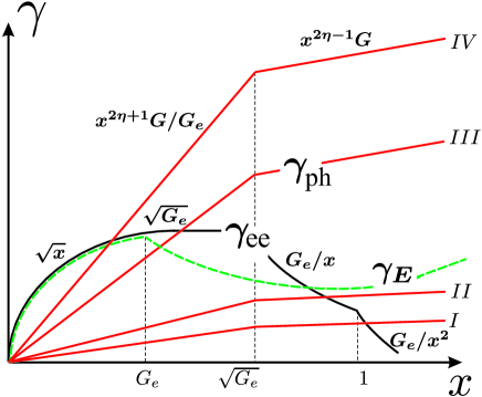
Figure 1: Schematic plot of the dimensionless electron-phonon scattering rate $\gamma_{\rm{ph}}(x)$ at $G_{e}\ll 1$ for four different values of $G$ ($G$ increases from I to IV). Also shown are the transport scattering rate $\gamma_{\rm{ee}}(x)$ (thick solid) and the energy relaxation rate $\gamma_{E}(x)$ (dashed) induced by electron-electron scattering.

Let us consider regimes I–IV (see Fig. 1) realized with increasing electron-phonon effective coupling $G$:

• I. $G\ll G_{e}.$ Electron-phonon coupling is weak and $\gamma_{\rm{ph}}\ll\gamma_{\rm{ee}}$ within relevant energy interval ($\epsilon<T,~{}x<1$), so that the phonon contribution to the transport rate is negligibly small and $\Sigma=1/G_{e}.$ Relevant energies are of the order of temperature, $x\sim 1.$

• II. $G_{e}\ll G\ll G_{e}^{1-\eta}.$ Electron-phonon contribution dominates, the screening of the phonons yields negligible effect, implying that $\Sigma=1/G$ and $x\sim 1$.

• III. $G_{e}^{1-\eta}\ll G\ll G_{e}^{1/2-2\eta}.$ The same as for regime II, $\Sigma=1/G$, $x\sim 1$.

• IV. $G_{e}^{1/2-2\eta}\ll G.$ The conductivity is determined by a competition between electron-electron collisions and screened electron-phonon interaction. The dominant contributions comes from low energies, $\ x\sim(G_{e}/G)^{2/1+4\eta}\ll 1$, where $\gamma_{\rm{ph}}\approx\gamma_{\rm{ee}}$. The dimensionless conductivity $\Sigma$ scales with the coupling constants as $\Sigma\sim(G_{e}/G)^{3/{1+4\eta}}.$

Consider now the opposite case $G_{e}\gg 1.$ Calculations analogous to the ones carried out in Ref. Schuett-ee, show that in this case, $\gamma_{\rm{ee}}\sim\sqrt{x}$ for all relevant energies ($x<1$). In the absence of phonons ($G=0$), the conductivity limited by electron-electron collisions is given byaleiner $\sigma\sim e^{2}N^{2}/\hbar$, and, consequently, $\Sigma\simeq 1$. For $G\neq 0$ one should also take into account phonons which are strongly screened in this case for all relevant energies, so that $\gamma_{\rm{ph}}\sim(G/G_{e})x^{2\eta+1}$ for $0<x<1$. The phonon scattering becomes important when $G$ becomes larger than $G_{e}$. The main contribution to the resistivity comes then from the region $x\sim(G_{e}/G)^{2/1+4\eta}\ll 1$, where $\gamma_{\rm{ee}}\sim\gamma_{\rm{ph}}$, yielding $\Sigma\sim(G_{e}/G)^{3/{1+4\eta}}$.

III.3 Results

The above results are summarized in Fig. 2, which illustrates different scattering regimes in the plane of parameters $G$ and $G_{e}$. In the regions (a) and (b) the phonon scattering is weak and the conductivity is limited by electron-electron collisions only. Contrary to this, in region (c) the electron-electron interaction is weak, the phonons dominate transport properties and their screening can be neglected. In the region (d), the conductivity is determined by competition between electron-electron collisions and scattering by screened phonons. As a result of this competition, a new energy scale appears in the problem, where contributions of both types of scattering are of the same order. Finally, on the boundary of the region (e), the conductivity achieves its “quantum limit” of the order of $e^{2}N/\hbar.$ We expect that the conductivity saturates at this value in the whole region (e).

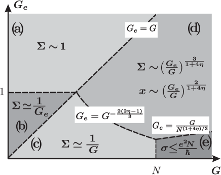
Figure 2: Conductivity of clean suspended graphene at the Dirac point. Transport regimes characterized by different behavior of dimensionless conductivity $\Sigma$ are shown in the parameter plane of effective (temperature-dependent) dimensionless couplings $G$ and $G_{e}$. The analytical expressions for dashed lines separating different regimes are given in the white boxes.

It is worth reminding the reader that all the temperature dependence has been absorbed into dimensionless constants $G$ and $G_{e}$. Since $G_{e}$ depends on $T$ in a very slow (logarithmic) manner, the dependence of $\Sigma$ (and, consequently, $\sigma$) on $T$ is mostly determined by power-law temperature dependence of $G$. The dependence of $\Sigma(G,G_{e})$ on $G$ for fixed $G_{e}$ is illustrated in Fig. 3 for the case of relatively small $G_{e}$ such that $(1/N)^{2(2\eta-1)/3}<G_{e}<1$. These inequalities correspond to a horizontal line in $(G,G_{e})$-plane (see Fig. 2) lying above the upper left corner of the region $(e)$ but below $G_{e}=1$. We see that at small $G$ (low temperatures) the electron-electron collisions dominate. At intermediate temperatures $\Sigma$ is limited by phonons ($\Sigma\simeq 1/G$) and at high temperatures the conductivity is determined by the narrow region of energies where electron-electron collisions and scattering on the screened phonons have approximately equal rates. In this region, $\Sigma\simeq\left({G_{e}}/{G}\right)^{{3}/{1+4\eta}}$. The perturbative calculations presented above become invalid at very high temperature, when $\Sigma$ drops down to $\sim 1/N$ and, consequently, $\sigma$ becomes of the order of the quantum limit $e^{2}N/\hbar$.

In order to make the picture complete, we also showed in Fig. 3 the contribution of a static disorder (if exists) assuming that it is due to randomly distributed charged impurities (another possible type of disorder in suspended graphene—adatoms—would lead to similar resultsimpurity ). Such disorder dominates at low temperatures when $G$ is small. Indeed, transport scattering rate due to charged impurities is inversely proportional to the energy $1/\tau_{\rm{im}}(\epsilon)\propto n_{i}/\epsilon$ (here $n_{i}$ is the impurity concentration) and at low $T$ exceeds electron-phonon and electron-electron scattering rates at relevant energies $\epsilon\sim T.$ The impurity-limited conductivity is estimated as $\sigma_{\rm{im}}\sim(e^{2}N/\hbar)T\tau_{\rm{im}}(T)\propto T^{2}/n_{i}$. This equation is valid provided that $T\tau_{\rm{im}}(T)\gg\hbar,$ which implies that temperature is not too small. With further lowering temperature, $\sigma_{\rm{im}}$ saturates at the value $e^{2}N/\hbar$ (see Refs. impurity, ; ostrovsky07, ; ostrovsky10, for the analysis of the nature of the corresponding quantum critical point and discussion of related issues such as localization or antilocalization). As illustrated in Fig. 3, impurity scattering becomes relevant when $\sigma_{\rm{im}}$ becomes smaller than conductivity limited by phonons and electron-electron collisions. The decay of the conductivity both at low and at high temperatures can be also understood in the following way. Since the phonon potential is quasistatic, it can be treated on equal footing with the impurity scattering. Hence one could incorporate the impurity scattering into the effective coupling constant $G$, which would then become a non-monotonic function of temperature $G\propto T^{\eta}+1/T$ (we omit temperature-independent coefficients). With decreasing temperature, ${G}$ defined in this way would first fall, then reach the minimum, and then start to grow again, so that both at very high and very low temperatures we would arrive at the region (e) (“quantum limit”) in Fig. 2.

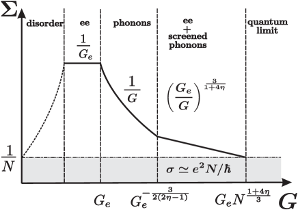
Figure 3: Dimensionless conductivity $\Sigma(G,G_{e})$ at the Dirac point as a function of effective phonon coupling $G$ for fixed small electron-electron coupling $G_{e}$. According to the definition of $G$, Eq. (44), the shown dependence can be also understood as temperature dependence of the resistivity. In the low-$G$ (low-temperature) region, the conductivity is governed by impurity scattering (shown by dashed line).

In the above analysis, we neglected contribution of other types of phonons. This can be contrasted with the previous publications, Mahan ; Manez ; CaKim ; Oppen-short ; Oppen-Scr where it was argued that the contribution of phonon-induced random vector potential might dominate over deformation potential. Let us estimate the contribution of the gauge phonon fields. From Eqs. (2) and (10), one finds the contribution of the flexural phonons to the gauge potential:

$$A_{x}=\partial_{x}h\partial_{y}h,~{}~{}A_{y}=[(\partial_{x}h)^{2}-(\partial_{y}h)^{2}]/2.$$ (53)

Similar to Eq. (11), gauge potential $V_{\mathbf{A}}$ is quadratic with respect to out-of-plane displacement of the graphene membrane. Also, analogously to deformation potential, the gauge field is quasistatic. Hence the scattering rate may be calculated by using the golden rule for scattering on the static potential $V_{\mathbf{A}}$. Proceeding in this way, we obtain

$$\gamma_{\rm{ph}}^{\mathbf{A}}\propto G_{\mathbf{A}}x^{2\eta-1}.$$ (54)

Equation (54) differs from the bottom line of Eq. (51) only by replacement of $G$ with a much smaller constant:

$$G_{\mathbf{A}}=G\left(\frac{g_{2}}{g_{1}}\right)^{2}\approx 2.5\times 10^{-3}G\,,$$ (55)

so that the scattering off the gauge field is much less efficient than that off the deformation potential. In fact, one should be slightly more careful at this point, since, in contrast to the deformation potential, the gauge field is not screened and Eq. (54) remains valid also at $x<\sqrt{G_{e}}$, where deformation potential scales as $1/G_{e}$ because of screening. Hence, with increasing $G_{e},$ gauge field may come into competition with deformation field. Specifically, for

$$G_{e}\gg\left(\frac{g_{1}}{g_{2}}\right)^{2}\approx 4\times 10^{2},$$ (56)

one could neglect the latter contribution, and the conductivity would be limited by a combined effect of the gauge field and electron-electron interaction. Simple estimates show, however, that the inequality Eq. (56) is hard to satisfy in realistic system, especially when the logarithmic renormalization of $g_{e}$ is taken into account. Furthermore, there is a second condition:

$$G\gg\left(\frac{g_{1}}{g_{2}}\right)^{2},$$ (57)

which ensures that the rate of electron-electron collisions is smaller than the gauge-field scattering rate. Only provided that both Eqs. (56) and (57) are satisfied (i.e. both $G$ and $G_{e}$ are very large), the resistivity is controlled by the scattering off the gauge field, $\Sigma=1/G_{\mathbf{A}}$. This situation appears highly unrealistic. We thus conclude that the gauge phonon field does not essentially affect transport properties of graphene in the Dirac point up to very high and unrealistic values of $G$ and $G_{e}$.

One can also check that in-plane phonons do not give essential contribution for realistic values of parameters. This is consistent with the previous study Oppen-long that came to the same conclusion for the case of large chemical potential $\mu$ in the absence of externally applied strain.

III.4 Phonon-induced velocity renormalization

In the previous sections we discussed the electron scattering rate caused by flexural phonons. Technically, this implied calculation of imaginary part of the electron self-energy in the quasistatic phonon potential. One may also calculate the real part of the self-energy, thus extracting information about a phonon-induced spectrum modification. This will allow us to verify the assumption that the electron spectrum is not changed essentially, which was implicit in our perturbative analysis.

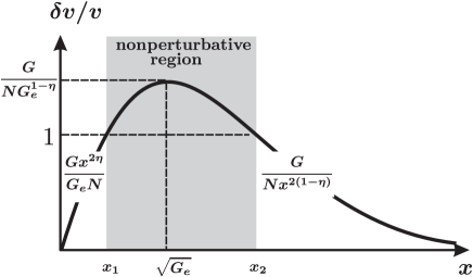
Figure 4: Velocity renormalization for $G_{e}\ll 1$ and $G/NG_{e}^{1-\eta}>1$

Simple calculations yield the following estimate for the energy-dependent velocity renormalization, $\delta v,$ caused by flexural phonons damped by the Thomas-Fermi screening:

$$\frac{\delta v}{v}\sim\left\{\begin{array}[]{ll}\displaystyle{\frac{G}{NG_{e}}x^{2\eta}},\qquad\text{for}~{}~{}x<\sqrt{G_{e}},\vspace{2mm}\\ \displaystyle{\frac{G}{N}\frac{1}{x^{2(1-\eta)}}},\qquad\text{for}~{}~{}x>\sqrt{G_{e}}.\end{array}\right.$$ (58)

Comparing Eq. (58) with Eq. (51), we see that

$$\frac{\delta v}{v}\sim\frac{\hbar}{\epsilon\tau_{\rm{tr}}},$$ (59)

so that the relative correction to the velocity is on the order of the scattering-induced spectrum smearing.

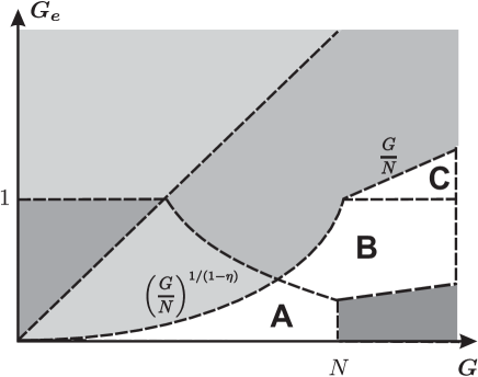
Figure 5: Regions A,B,C where a “non-perturbative” interval of energies exists

In most of the cases, spectrum correction is small, $\delta v/v\ll 1,$ in the whole relevant energy interval $x\leq 1$, and thus harmless. However, in certain domains of parameters, the estimate (58) ceases to be small. This may indicate that the calculation of the conductivity within the lowest order of the perturbation theory (Born approximation) may become insufficient.

Specifically, for $G_{e}>1$ we have ${\delta v}/{v}\simeq({G}/{NG_{e}})x^{2\eta}$ at $x\leq 1$, so that the maximal value of ${\delta v}/{v}$ is achieved at $x\sim 1$: ${\delta v_{\rm{max}}}/{v}\sim{G}/{NG_{e}}$. We thus conclude that “nonperturbative” effects (i.e. those going beyond the Born approximation) might show up for $G_{e}<G/N.$

Consider now the opposite case $G_{e}<1,$ when the relative correction reaches the maximum

$$\frac{\delta v_{\rm{max}}}{v}\sim\frac{G}{NG_{e}^{1-\eta}}$$ (60)

at $x\simeq\sqrt{G_{e}}.$ Hence, “nonperturbative” effects come now into play for $G_{e}<(G/N)^{1/(1-\eta)},$ as illustrated in Fig. 4. From this estimates, we find the regions on the plane $(G,G_{e})$ for which $\delta v/v>1$ at some energy interval (but at the same time $\sigma>e^{2}N/\hbar$). These regions are marked as A,B, and C on Fig. 5. In the regions A and B, the velocity correction is not small in the interval $x_{1}<x<x_{2},$ where $x_{1}=(G_{e}N/G)^{1/2\eta}$ and $x_{2}=(G/N)^{1/2(1-\eta)}$. One may expect that this “nonperturbative energy strip” does not affect conductivity in the region A, because the width of this strip $x_{2}-x_{1}$ is much smaller than the temperature window: $x_{2}-x_{1}\ll 1$. Analogously, the perturbative analysis is expected to give the correct result in region C, because $\delta v/v\ll 1$ in the range $x\sim(G_{e}/G)^{2/(1+4\eta)},$ which is determined by the condition $\gamma_{\rm{ph}}\sim\gamma_{\rm{ee}}$ and governs the resistivity within the perturbative calculation (see previous section). On the other hand, a controlled calculation of the conductivity in the region B requires going beyond the Born approximation.

The discussion of such “nonperturbative” phenomena is out of scope of the current work and we restrict ourselves to a short comment of a somewhat speculative character. One may expect that the system becomes strongly inhomogeneous, i.e., it can be characterized by a local chemical potential $\mu(\mathbf{r})$ showing large fluctuations around zero (with large number of electrons within each such “puddle”). Such fluctuations can be described in the framework of random resistor network, which involves percolation physics.cheianov Also, within a spatial scale where $\mu(\mathbf{r})$ is homogeneous, the spectrum of electrons and holes might be essentially different from the linear one.comment This and related issues will be discussed elsewhere.

IV Away from the Dirac point:   finite $\mu$

In Sec. III, we considered conductivity at the Dirac point ($\mu=0$), which is in the main focus of this paper. In the present section, we briefly discuss the behavior of conductivity away from the Dirac point, $\mu\neq 0$. The phonon-limited resistivity in this regime has been previously analyzed in Refs. Oppen-long, and Ochoa, where the renormalization of $\varkappa$ was neglected. While this is justified in the presence of sufficiently strong externally induced tension, the renormalization essentially affects the scattering rate when tension is absent (or weak), see Sec. II. Below we explore the effect of flexural phonons on resistivity of graphene at nonzero $\mu$ in the absence of tension, with taking into account the anharmonic renormalization.

First, we ignore the electron-electron interaction. Substituting Eq. (II.2) into Eq. (27), we get

$$\sigma_{\rm{ph}} = \frac{e^{2}}{\hbar}\frac{N}{g^{2}}$$ (61)

$$\times \left\{\begin{array}[]{ll}\displaystyle{\frac{C_{1}}{16Z^{2}C}\left(\frac{\Delta_{c}}{T}\right)^{\eta}},&\text{for}~{}|\mu|\ll T,\vspace{2mm}\\ \displaystyle{\frac{1}{8CZ^{2}}\left(\frac{\Delta_{c}}{T}\right)^{\eta}\left(\frac{\mu}{T}\right)^{2-2\eta}},&\text{for}~{}T\ll|\mu|\ll\sqrt{T\Delta_{c}},\vspace{2mm}\\ \displaystyle{\frac{1}{8}\left(\frac{\mu}{{T}}\right)^{2}\frac{1}{\ln(\mu/\sqrt{T\Delta_{c}})}},&\text{for}~{}\sqrt{T\Delta_{c}}\ll|\mu|\,.\end{array}\right.$$ (65)

We see that the conductivity increases with $\mu$ as $\mu^{2-2\eta}\simeq\mu^{0.56}$ for $T\ll\mu\ll\sqrt{T\Delta_{c}}$ and as $\mu^{2}/\ln\mu$ for $\sqrt{T\Delta_{c}}\ll\mu.$

Now we include the Coulomb interaction into consideration. Just as in the case $\mu=0$ (Sec. III), its role is twofold: first, it screens the deformation potential and, second, it opens an additional (electron-electron) channel of scattering.

For $\mu\ll T$ [first line in Eqs. (61)], the effect of the screening was discussed in the previous sections [see Eqs. (102)–(106) and (46)]. For $\mu\gg T,$ the Thomas-Fermi screening leads to the renormalization of $g$ (see Ref. Oppen-long, ) described by Eq. (45) with

$$\Pi(Q)=\frac{\mu}{2\pi\hbar^{2}v^{2}}.$$ (66)

Thus, we have to replace

$$g\to\frac{g}{1+g_{e}Nk_{F}/Q},$$ (67)

where $k_{F}=\mu/\hbar v.$ The transport scattering rate is calculated in Appendix A.3. For $G_{e}\ll 1$ screening can be neglected so that $1/\tau_{\rm{tr}}$ and $\sigma_{\rm{ph}}$ are given by Eqs. (II.2) and (61), respectively. For $G_{e}\gg 1,$ scattering rate reads

$$\frac{1}{\tau_{\rm{tr}}(\epsilon)} \simeq \frac{2g^{2}T^{2}|\epsilon|}{\pi\hbar G_{e}\mu^{2}}$$ (68)

$$\times \left\{\begin{array}[]{ll}\displaystyle{C_{3}\ln\left(\frac{|\epsilon|}{\sqrt{T\Delta_{c}}}\right)},&\text{for}~{}~{}|\epsilon|\gg\sqrt{T\Delta_{c}},\vspace{2mm}\\ \displaystyle{\tilde{C}Z^{2}~{}\left(\frac{|\epsilon|}{\sqrt{T\Delta_{c}}}\right)^{2\eta}},&\text{for}~{}~{}|\epsilon|\ll\sqrt{T\Delta_{c}}\,,\end{array}\right.$$ (71)

where $\tilde{C}\approx 4.$ Then, for $G_{e}\gg 1,$ the conductivity limited by screened flexural phonons takes the form

$$\sigma_{\rm{ph}} \simeq \frac{e^{2}}{\hbar}\frac{NG_{e}}{g^{2}}$$ (72)

$$\times \left\{\begin{array}[]{ll}\displaystyle{\frac{1}{8\tilde{C}Z^{2}}\left(\frac{\Delta_{c}}{T}\right)^{\eta}\left(\frac{\mu}{T}\right)^{2-2\eta}},~{}\text{for}~{}T\ll|\mu|\ll\sqrt{T\Delta_{c}},\vspace{2mm}\\ \displaystyle{\frac{1}{8}\left(\frac{\mu}{{T}}\right)^{2}\frac{1}{C_{3}\ln(\mu/\sqrt{T\Delta_{c}})}},~{}\text{for}~{}\sqrt{T\Delta_{c}}\ll|\mu|.\end{array}\right.$$ (75)

Finally, we discuss the role of electron-electron collisions at $\mu\neq 0$. General equations describing the competition between electron-electron collisions and electron-phonon scattering for arbitrary $\mu$ are derived in Appendix B. As follows from these results, for $\mu\gg T$ electron-electron collisions do not contribute to effective scattering rate and the conductivity is given by Eq. (72). This implies that the electron-phonon scattering becomes even more important when the chemical potential is tuned away from the Dirac point. This conclusion is supported by consideration of the conductivity in the region $0<\mu\ll T$ for the case, when electron-electron collisions dominate at $\mu=0.$ As shown in Appendix B, the conductivity is given in this case by

$$\sigma\sim\frac{e^{2}NT}{\hbar}\langle 1\rangle\left[\frac{1}{\langle 1/\tau_{\rm{ee}}\rangle}+\frac{\mu^{2}}{T^{2}}\frac{1}{\langle 1/\tau_{\rm{ph}}\rangle}\right].$$ (76)

(here we omit numerical coefficients of order unity). We see that the electron-phonon scattering, being weak at $\mu=0$, becomes nevertheless dominant at a quite small chemical potential $\mu\sim T\sqrt{\langle 1/\tau_{\rm{ph}}\rangle/\langle 1/\tau_{\rm{ee}}\rangle}\ll T.$ The behavior of the dimensionless conductivity $\Sigma$ with increasing temperature for $\mu\neq 0$ is shown schematically in Fig. 6. It is assumed in this figure that $\mu$ is relatively small, so that the temperature-dependent coupling constant $G=G[T]$ is weak for $T\sim\mu$ as compared to the coupling constant $G_{e}[T]$ (which depends only logarithmically weakly on temperature),

$$G[\mu]\ll G_{e}[\mu]\,.$$ (77)

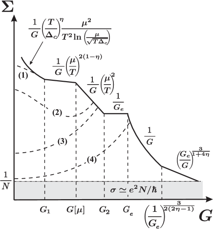
Figure 6: Temperature dependence of dimensionless conductivity $\Sigma$ for $G_{e}\ll 1$ and relatively small $\mu$ such that $G[\mu]\ll G_{e}$. Dashed lines show conductivity limited by charged impurities for different impurity concentration increasing from the curve (1) to the curve (4).

For $G[T]\ll G_{2}$ (here $G_{2}=G[T_{2}]$ and $T_{2}\gg\mu$ should be found from the equation $G[T_{2}]=G_{e}\mu^{2}/T_{2}^{2}$) the conductivity is limited by screened phonons. For very small $G$ such that $G\ll G_{1}=G[\mu^{2}/\Delta_{c}],$ the phonons can be treated in the harmonic approximation. For $G\gg G_{2}$ the temperature dependence is the same as in Fig. 3. At lowest temperatures the conductivity is limited by the scattering off static disorder (charged impurities) as illustrated in Fig. 6 by dashed lines corresponding to different impurity concentrations. Indeed, the phonon transport rate, Eq. (68), taken at $\epsilon=\mu,$ has a maximum as a function of $\mu$ at $\mu\approx\sqrt{T\Delta_{c}}$ and the maximal value decreases with decreasing the temperature as $T^{3/2}.$ Therefore, at sufficiently low temperatures scattering by charged impurities with the temperature-independent rate, $1/\tau_{\rm{im}}\propto n_{i}/|\epsilon|\approx n_{i}/\mu,$ dominates within the relevant energy interval:

$$\frac{1}{\tau_{\rm{im}}(\epsilon)}\gg\frac{1}{\tau_{\rm{tr}}(\epsilon,T)},~{}~{}\text{for}~{}|\epsilon-\mu|\lesssim T.$$ (78)

Here $\tau_{\rm{tr}}(\epsilon,T)$ is the phonon-induced transport time given by Eq. (II.2) or Eq. (68); it is convenient for our purposes to write it as a function of two variables $\epsilon$ and $T.$ The impurity scattering time $\tau_{\rm{im}}$ is in fact also a function of two independent variables $\epsilon$ and $T$ because of screening of the impurity potential. This effect does not change qualitatively our results, so that we do not discuss it here.

Let us find the temperature behavior of the impurity-dominated conductivity assuming that Eq. (78) is satisfied. As discussed above, electron-electron collisions become irrelevant while going away from the Dirac point, so that we neglect them and write the conductivity as

$$\sigma=\frac{e^{2}N}{16\pi\hbar^{2}}\times$$ (79)

$$\int_{-\infty}^{\infty}d\epsilon\frac{|\epsilon|}{T\cosh^{2}[(\epsilon-\mu)/2T]}\frac{\tau_{\rm{tr}}(\epsilon,T)\tau_{\rm{im}}(\epsilon)}{\tau_{\rm{im}}(\epsilon)+\tau_{\rm{tr}}(\epsilon,T)}.$$

Using Eq. (78) we expand Eq. (79) over power of $\tau_{\rm{im}}/\tau_{\rm{tr}}$ and keep terms of the zero and first order:

$$\sigma=\frac{e^{2}N}{16\pi\hbar^{2}}\int_{-\infty}^{\infty}d\epsilon\frac{|\epsilon|\left[\tau_{\rm{im}}(\epsilon)-{\tau_{\rm{im}}^{2}(\epsilon)}/{\tau_{\rm{tr}}(\epsilon,T)}\right]}{T\cosh^{2}[(\epsilon-\mu)/2T]}.$$ (80)

Since $T\ll\mu,$ the integrand is peaked near the region $\epsilon\approx\mu.$ While calculating contribution of the first term in the square brackets we write $|\epsilon|\tau_{\rm{im}}(\epsilon)\approx\mu\tau_{\rm{im}}(\mu)+[\mu\tau_{\rm{im}}(\mu)]^{\prime}(\epsilon-\mu)+[\mu\tau_{\rm{im}}(\mu)]^{\prime\prime}(\epsilon-\mu)^{2}/2.$ The second term in the square brackets of Eq. (80) is small and while integrating it we neglect temperature broadening of the Fermi-function. Doing so, we find for the temperature-dependent part of the conductivity,

$$\delta\sigma = \sigma(T)-\sigma(0)$$

$$= \frac{e^{2}N}{4\pi\hbar^{2}}\left\{\frac{\pi^{2}T^{2}}{6}[\mu\tau_{\rm{im}}(\mu)]^{\prime\prime}-\frac{\mu\tau_{\rm{im}}^{2}(\mu)}{\tau_{\rm{tr}}(\mu,T)}\right\}.$$

This equation is valid for an arbitrary type of impurity scattering. For charged impurities we find that $\delta\sigma$ is given as a sum of two terms of different signs:

$$\delta\sigma(T)\propto\frac{T^{2}}{n_{i}}-\frac{\mu^{3}}{n_{i}^{2}}\frac{1}{\tau_{\rm{tr}}(\mu,T)}$$ (82)

(here we omit coefficients which do not depend on $\mu,T$ and $n_{i}$). The analysis of Eq. (82) shows that “metallic” behavior of conductivity (i.e. its increase with lowering $T$) at low $n_{i}$ changes to an “insulating” one with increasing $n_{i}$ as illustrated in Fig. 6 by dashed lines. Alternatively, this crossover in the behavior of conductivity at relatively lower temperatures can be observed if one changes $\mu$ at fixed disorder. One can also see from Fig. 6 that at intermediate values of $n_{i}$ (or of $\mu$) the dependence of conductivity on $T$ may have two maxima [see curve (2) in Fig. 6].

V Comparison to experiment

We now compare our results with available experimental data Bolotin (see also Ref. Ochoa, ). To this end, we plot conductivity as a function of temperature and chemical potential (or, equivalently, electron concentration) for the same values of parameters as in Ref. Bolotin, . We assume that electron-electron coupling is renormalized from the value $g_{e}^{0}$ at large energies ($\sim\Delta$) to $g_{e}\simeq 1$ in the room temperature interval, so that $G_{e}=C_{3}g_{e}^{2}N^{2}\simeq 16\gg 1$. The conductivity is obtained by interpolating of equation for total scattering rate (which is the sum of the electron-electron, electron-phonon, and impurity scattering rates) between asymptotical expressions presented in the previous sections and by substituting thus found rate into the Drude formula Eq. (26). The main purpose of such an interpolation is to estimate characteristic values of conductivity and analyze qualitatively the dependence of $\sigma$ on $\mu,T$ and $n_{i}.$ Due to evident reasons, we do not pretend to get quantitative agreement with experiment. First of all, interpolation procedure yields numerical value of conductivity up to the coefficient on the order of unity at the boundaries separating regions of parameters corresponding to different transport regimes. Second, even asymptotical expressions contain some unknown numerical coefficients. In particular, the coefficient $Z\sim 1$ entering the phonon correlation function [see Eq. (22)] is not known as it was discussed above. Below we use $Z=2,$ which allows us to get reasonable agreement with experiment. We also do not know the numerical coefficient in the equation $\gamma_{\rm{ee}}\sim\sqrt{x}$ for dimensionless electron-electron scattering rate in the limit $G_{e}\gg 1.$ In the estimates we choose this coefficient to be $1/4$ which yields a best fit to experimental data. Another issue, which was not resolved rigourously, is the screening of the impurity potential. In the estimates we simply assume $1/\tau_{\rm{im}}\sim e^{4}n_{i}/|\epsilon|\kappa$ and choose the coefficient in this equation to be unity. This yields a good approximation for impurity scattering rate (up to a numerical coefficient) at least for not too low temperatures, when conductivity is much larger than $e^{2}/h.$

At the Dirac point the data shown in Fig.4 of Ref. Bolotin, show an increase of conductivity by factor of $2\div 3$ when temperature increases from 5 to 200 K, with a clear saturation around 200 K. Let us compare this picture with theoretical estimates. The calculated conductivity at the Dirac point is plotted in Fig. 7 for different values of impurity concentration $n_{i}$. A curve corresponding to $n_{i}=0.5\times 10^{10}\text{cm}^{-2}$ (third curve counted from the bottom) reasonably agrees with experiment. A similar behavior with a somewhat larger ratio $\sigma(200\>{\rm K})/\sigma(5\>{\rm K})$ is seen in Fig. 3 of Ref. Ochoa, . We expect that with further increase of temperature the conductivity will drop due to electron-phonon scattering, as found in Sec. III of the present work and is shown schematically in our Fig. 3. As seen from Fig. 7, the drop of the conductivity with $T$ can be observed at smaller $T$ provided that one uses cleaner samples.

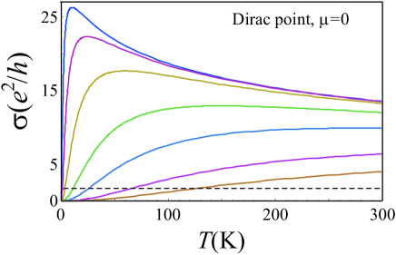
Figure 7: Conductivity at the Dirac point ($\mu=0$) for different values of the impurity concentration ($n_{i}/10^{10}~{}\text{cm}^{-2}=10^{-4},~{}10^{-3},~{}10^{-2},~{}10^{-1},~{}0.5,~{}3,~{}10$) increasing from the top to the bottom. Dashed line corresponds to SCBA limit $\sigma=4e^{2}/\pi h.$ Calculations are controlled only well above this line.

Let us note that the conductivity curves in Fig. 7 go to zero in the limit $T\to 0,$ in view of the vanishing density of states at the Dirac point. If we would include disorder-induced level broadening self-consistently [in the framework of the self-consistent Born approximation (SCBA)], we would get instead a limiting conductivity value $4e^{2}/\pi h$ (marked by a horizontal dashed line in the plots). The actual behavior of conductivity in this regime is controlled by quantum interference effects that lead to localization, antilocalization, or quantum criticality, depending on the character of disorder.ostrovsky07 In the present paper we do not discuss these phenomena, as our focus is on regimes where the dimensionless conductivity is sufficiently large and quantum interference corrections do not change it significantly.

When one moves away from the Dirac point, the experimentally observed temperature dependence changes (see Fig.2 of Ref. Bolotin, ), and at sufficiently large $\mu$ the conductivity becomes monotonously decreasing function of $T$. This evolution is in a very good qualitative agreement with our results. To see this, we fixed the impurity concentration at the level $n_{i}=0.5\times 10^{10}\text{cm}^{-2}$, and calculated resistivity (just as in Fig.2 of Ref. Bolotin, ) as a function of the electron concentration $n=N\mu^{2}/4\pi\hbar^{2}v^{2}$ for different values of temperature (the same as used in Ref. Bolotin, ). The results are plotted in Fig. 8 and look very similar to the ones presented in Fig.2 of Ref. Bolotin, .

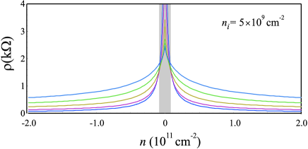
Figure 8: Resistivity as a function of electron concentration at $n_{i}=5\times 10^{9}~{}\text{cm}^{-2}$ and different temperatures ($T/1\text{K}=5,~{}40,~{}90,~{}150,~{}230$) increasing from the bottom to the top at large $n$. Within the grey area temperature dependence is “insulating”, while outside this region it is “metallic”.

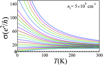
Figure 9: Conductivity at fixed impurity concentration ($n_{i}=5\times 10^{9}~{}\text{cm}^{-2}$) for different values of chemical potential ($\mu/1\text{K}=0$, 50, 70, 90, 110, 130, 150, 170, 190, 210, 230, 250, 270, 290, 310, 330, 350, 400, 450, 500, 550, 600) increasing from the bottom to the top. Dashed line corresponds to SCBA limit $\sigma=4e^{2}/\pi h.$

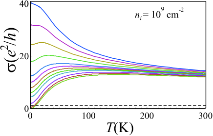
Figure 10: Conductivity at fixed impurity concentration ($n_{i}=10^{9}~{}\text{cm}^{-2}$) for different values of chemical potential ($\mu/1~{}\text{K}=0,~{}10,~{}20,~{}30,~{}35,~{}40,~{}45,~{}50,~{}60,~{}70,~{}80,~{}90$) increasing from the bottom to the top. Dashed line corresponds to SCBA limit $\sigma=4e^{2}/\pi h.$

Within the grey area temperature dependence is “insulating”, while outside this region it is “metallic”. One of the main features of this picture is the existence of the “stationary” point, where $T$-dependence changes. To illustrate the existence of this point in a more transparent way we plotted in Figs. 9 and 10 the conductivity as a function of temperature for fixed impurity concentration and different values of the chemical potential. The “stationary” point in Fig. 8 corresponds to existence of more or less horizontal lines in Figs. 9 and 10 separating regions with “metallic” and “insulating” behavior. As seen from Figs. 9 and 10, the transition between different types of T-dependence becomes more pronounced with decreasing the impurity concentration. It is worth noting that the transition may be also obtained for fixed $\mu$ by changing the impurity concentration (for example, by annealing the sample) as illustrated in Fig. 11.

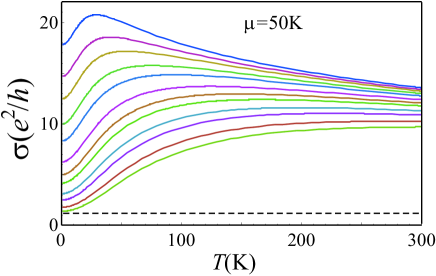
Figure 11: Conductivity at $\mu=50$ K for different values of the impurity concentration ($n_{i}/10^{10}~{}\text{cm}^{-2}=0.07,~{}0.085,~{}0.1,~{}0.125,~{}0.15,~{}0.2,~{}0.25,~{}0.3,~{}0.4,~{}0.5,~{}0.7,~{}0.9$) increasing from the top to the bottom. Dashed line corresponds to SCBA limit $\sigma=4e^{2}/\pi h.$

Sufficiently far from the Dirac point, such that $\mu\gg T$ for all relevant temperatures, only the first two phonon-controlled regimes of Fig. 6 survive, implying a crossover from the conductivity scaling $\sigma\propto\mu^{2}/T^{2}\ln(\mu^{2}/T\Delta_{c})$ at lower temperatures ($T\ll\mu^{2}/\Delta_{c}$) to $\sigma\propto\mu^{2-2\eta}/T^{2-\eta}$ at higher temperatures $T\gg\mu^{2}/\Delta_{c}$. However, the temperature, separating two regimes, $\mu^{2}/\Delta_{c},$ turns out to be very small, on the order of $1$ K, even for largest chemical potentials, $\mu\simeq 600$ K, studied in Ref. Bolotin, . In other words, experimental situation corresponds to anharmonic regime. While the data shown in Fig. 3 of Ref. Bolotin, do indicate a power-law increase of resistivity with temperature (at relatively large temperature), the exponents do not quite agree: the theoretical dependence, $\rho\sim T^{2-\eta}\sim T^{1.3}$ [see upper line of Eq. (72)], turns out to be slightly stronger than experimentally observed linear one, $\rho\sim T.$

Consider now the dependence of the conductivity on the electron density. As observed in Ref. Bolotin, , this dependence is qualitatively different in clean and dirty samples. When impurity concentration is large, conductivity is a linear function of the concentration, $\sigma\sim n,$ while at the same sample after annealing the dependence becomes sublinear: $\sigma$ increases with electron density $n\propto\mu^{2}$ with an exponent considerably smaller than unity, which is at least in qualitative agreement with the $\sigma\propto\mu^{2-2\eta}\propto n^{1-\eta}$ predicted above for transport away from the Dirac point [see upper line of Eq. (72)]. This is illustrated in Fig. 12, where $\sigma$ is plotted as function of $n$ for fixed temperature, $T=40$ K (the same as in Ref. Bolotin, ), and two different values of the impurity concentration. This picture looks very similar to the Fig. 1 in Ref. Bolotin, . Physically, the linear dependence at large $n_{i}$ is caused by impurity scattering, while sublinear one at low $n_{i}$ is due to the phonon scattering.

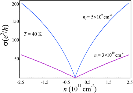
Figure 12: Conductivity as a function of electron concentration at $T=40$ K and two different values of impurity concentration: $n_{i}=5\times 10^{9}~{}\text{cm}^{-2}$ and $n_{i}=3\times 10^{10}~{}\text{cm}^{-2}.$

Finally, we make a rough estimates of the numerical values of the conductivity. For this purpose, we consider temperature dependence of the conductivity for $n_{i}=0.5\times 10^{10}\text{cm}^{-2}$ and different values of $\mu$ (see Fig. 9). For $\mu=600\>{\rm K}$ (which corresponds to the highest density $n_{e}=2\times 10^{11}\>{\rm cm}^{-2}$ studied in Ref. Bolotin, ) and $T=200\>{\rm K}$ (which is approximately the highest temperature in Ref. Bolotin, ) theoretical prediction is $\sigma\simeq 50e^{2}/h$ (upper curve in Fig. 9). In the Dirac point theory predicts $\sigma\simeq 9e^{2}/h$ (lowest curve in Fig. 9). The experimental data of Ref. Bolotin, yield $\sigma\simeq 70e^{2}/h$ for $\mu=600\>{\rm K}$ and $\sigma\simeq 12e^{2}/h$ for $\mu=0$, in reasonable agreement with our findings.

It was suggested in Refs. Oppen-long, ; Ochoa, that the experimental data of Refs. Bolotin, ; Ochoa, might be to some extent affected by strain that may result from fixing the sample at the contacts. It is worth emphasizing that in the present paper we have studied the case of a strain-free graphene and obtained reasonable qualitative agreement with experiment. Furthermore, the strength of the tension depends on the procedure of preparation of a sample. In particular, the built-in tensions in freely suspended graphene monolayers produced by means of chemical reduction of graphene oxide were found tension to be considerably weaker than in mechanically exfoliated graphene samples.

VI Summary

To conclude, we have studied transport in suspended clean graphene in a broad range of temperatures. We have explored the interplay of electron-phonon and electron-electron interactions and have found that the scattering off flexural phonons controls the resistivity at relatively high $T.$ Taking into account the anharmonic coupling of flexural and in-plane phonons was crucial for correct evaluation of the graphene conductivity.

Our results for the conductivity can be expressed in terms of two dimensionless coupling constants $G$ and $G_{e}$, characterizing the strength of the electron-phonon and electron-electron scattering, respectively. Both constants depend on temperature: $G$ shows a power-law scaling, $G\sim T^{\eta}$, with the exponent $\eta$ describing the scaling of the bending rigidity of graphene membrane with the length scale due to anharmonicity, while $G_{e}$ slowly (logarithmically) changes with $T$ due to renormalization of the Fermi velocity caused by electron-electron interaction.

At the Dirac point, the dimensionless conductivity $\Sigma(G,G_{e})$ of clean suspended graphene depends on $T$ only through temperature dependence of $G$ and $G_{e}.$ At low temperatures, $G<G_{e}$ and phonon scattering is negligible. In the room temperature interval $G\gg G_{e}$ and transport is dominated by phonon scattering. At sufficiently high temperatures one should take into account screening of the deformation potential due to electron-electron interaction. The overall “phase diagram” of scattering regimes and conductivity scaling of clean graphene at the Dirac point is shown in Fig. 2. A characteristic temperature dependence of conductivity is shown in Fig. 3. There, we also included the regime of low temperatures where the resistivity is controlled by disorder. [The lowest temperatures where quantum criticality or localization (antilocalization) effects come into play are not considered in this paper, see Refs. impurity, ; ostrovsky07, ; ostrovsky10, .] As seen in this figure, the conductivity first increases with $T$ (disorder-dominated regime), then shows a plateau (electron-electron scattering), and then drops due to electron-phonon scattering. In the high-temperature part of the latter regime, the Thomas-Fermi screening of phonons becomes important. Remarkably, at still higher temperatures the system enters the ultimate quantum regime (conductivity of the order of $e^{2}/h$ analogous to the one at lowest temperatures). In view of the quasistatic nature of flexural phonons, quantum interference phenomena are expected to be relevant in this regime, despite rather high temperatures.

Away from the Dirac point ($\mu\neq 0$), the role of the electron-phonon interaction increases as compared to the electron-electron one (since the latter conserves momentum). In particular, the electron-phonon scattering, even if weak at $\mu=0$, becomes dominant at a quite small $\mu$ such that $\mu\ll T$ [see Eq. (76)]. The temperature dependence of conductivity away from the Dirac point is sketched in Fig. 6. We also discuss the effect of static disorder (assuming for definiteness that charged impurities are the main source of disorder) as shown by dashed lines in Fig. 6. With increasing $\mu$ (or, else, with lowering impurity concentration at fixed nonzero $\mu$), the behavior of the Drude conductivity in the disorder-controlled low-temperature regime changes from “insulating” ($\sigma$ decreases at lowering $T$) to “metallic.”

Our findings qualitatively agree with experimental data of Refs. Bolotin, and Ochoa, , see Sec. V and Figs. 7–12. We hope that the results of this paper will stimulate further experimental investigations of conductivity of suspended graphene, including a systematic investigation of temperature dependence at different chemical potentials for $T$ up to (or even higher than) room temperature.

A number of problems related to this research have been left open. First, this includes the possibility of essentially non-Born and of “ultimate quantum” regimes at high temperatures at the Dirac point. Second, the detailed analysis of the scattering by charged impurities with the account of self-consistent screening is required. It is also interesting to study the effect of flexural phonons on quantum transport in suspended graphene in transverse magnetic fields.

VII Acknowledgments

We thank A.P. Dmitriev, F. Evers, F. von Oppen, J. Schmalian, and M. Schütt for useful discussions. The work was supported by RFBR, by programs of the RAS, by DFG CFN, DFG SPP “Graphene”, and by BMBF.

Appendix A Calculation of scattering rate

In this Appendix, we present a derivation of the transport time due to scattering off flexural phonons.

A.1 Harmonic approximation

We first neglect the anharmonicity. The quasistatic random potential representing approximately the displacement field of flexural phonons has the form:

$$V(\mathbf{r})=\frac{g_{1}T}{\varkappa S}\sum_{\mathbf{q}_{1},\mathbf{q}_{2}}\frac{\mathbf{q}_{1}\mathbf{q}_{2}}{q_{1}^{2}q_{2}^{2}}\sin(\mathbf{q}_{1}\mathbf{r}+\varphi_{\mathbf{q}_{1}})\sin(\mathbf{q}_{2}\mathbf{r}+\varphi_{\mathbf{q}_{2}}).$$ (83)

[Eq. (83) is obtained by substitution of Eq. (13) into Eq. (11).] Averaging squared matrix element of transition between $\psi_{\mathbf{k},\alpha}$ and $\psi_{\mathbf{k}^{\prime},\beta}$ over the phases $\varphi_{\mathbf{q}},$ we find that $\mathbf{k}^{\prime}=\mathbf{k}\pm\mathbf{q}_{1}\pm\mathbf{q}_{2},$ where all four combinations of $+$ and $-$ in front of $\mathbf{q}_{1}$ and $\mathbf{q}_{2}$ should be taken into account:

$$\langle|V_{\mathbf{k},\mathbf{k}^{\prime}}^{\alpha,\beta}|^{2}\rangle_{\varphi_{\mathbf{q}}}=\frac{g_{1}^{2}T^{2}}{8\varkappa^{2}S^{2}}\sum_{\mathbf{q}_{1},\mathbf{q}_{2},\pm}\frac{(\mathbf{q}_{1}\mathbf{q}_{2})^{2}}{q_{1}^{4}q_{2}^{4}}|\langle\chi_{\mathbf{k}}^{\alpha}|\chi_{\mathbf{k}^{\prime}}^{\beta}\rangle|^{2}\delta_{\mathbf{k}^{\prime},\mathbf{k}\pm\mathbf{q}_{1}\pm\mathbf{q}_{2}}\,.$$ (84)

The transport scattering rate for an electron in the branch $\alpha$ with the energy $\epsilon=\alpha vk$ is given by

$$\frac{1}{\tau_{\rm{tr}}^{\alpha}(\epsilon)} = \frac{\pi g_{1}^{2}T^{2}}{4\hbar\varkappa^{2}}\sum_{\pm,\beta}\int\frac{d^{2}\mathbf{q}_{1}}{(2\pi)^{2}}\frac{d^{2}\mathbf{q}_{2}}{(2\pi)^{2}}|\langle\chi_{\mathbf{k}}^{\alpha}|\chi_{\mathbf{k}\pm\mathbf{q}_{1}\pm\mathbf{q}_{2}}^{\beta}\rangle|^{2}$$

$$\times \frac{(\mathbf{q}_{1}\mathbf{q}_{2})^{2}}{q_{1}^{4}q_{2}^{4}}\delta(\epsilon^{\beta}_{\mathbf{k}\pm\mathbf{q}_{1}\pm\mathbf{q}_{2}}-\epsilon^{\alpha}_{\mathbf{k}})(1-\mathbf{n}_{\mathbf{k}}\mathbf{n}_{\mathbf{k}\pm\mathbf{q}_{1}\pm\mathbf{q}_{2}}).$$

In the quasielastic approximation, $\alpha=\beta$ due to delta-function in Eq. (A.1) and ${\tau_{tr}}$ is the function of $|\epsilon|=vk.$ Taking into account that the dominant contribution to the integral comes from the region where one of the momenta is much smaller than another one, say $q_{2}\ll q_{1},$ and using $|\langle\chi_{\mathbf{k}}^{\alpha}|\chi_{\mathbf{k}^{\prime}}^{\alpha}\rangle|^{2}=(1+\mathbf{n}_{\mathbf{k}}\mathbf{n}_{\mathbf{k}^{\prime}})/2$, we reduce Eq. (A.1) to the form

$$\frac{1}{\tau_{\rm{tr}}(\epsilon)} = \frac{\pi g_{1}^{2}T^{2}}{8\hbar\varkappa^{2}}\sum_{\pm,\beta}\int\frac{dq_{2}}{2\pi q_{2}}\frac{d^{2}\mathbf{q}_{1}}{(2\pi)^{2}q_{1}^{2}}$$ (86)

$$\times \delta(\epsilon^{\alpha}_{\mathbf{k}\pm\mathbf{q}_{1}}-\epsilon^{\alpha}_{\mathbf{k}})[1-(\mathbf{n}_{\mathbf{k}}\mathbf{n}_{\mathbf{k}\pm\mathbf{q}_{1}})^{2}].$$

Using the identity

$$\delta(k-|\mathbf{k}+\mathbf{q}|)={\delta(q-2k\cos\varphi)}/{|\cos\varphi|}$$ (87)

(here $\varphi$ is the angle between $\mathbf{q}$ and $\mathbf{k}$), we get

$$\frac{1}{\tau_{\rm{tr}}(\epsilon)} = \frac{g_{1}^{2}T^{2}}{32\pi^{2}\hbar^{2}\varkappa^{2}v}\int\frac{dq_{2}}{q_{2}}\int\frac{dq_{1}}{q_{1}}\int_{-\pi/2}^{\pi/2}d\varphi$$ (88)

$$\times \frac{\delta(q_{1}-2k\cos\varphi)}{\cos\varphi}(1-\cos^{2}2\varphi)\,.$$

Finally, taking also into account contribution of the region $q_{2}\gg q_{1}$, we obtain

$$\frac{1}{\tau_{\rm{tr}}(\epsilon)}=\frac{g_{1}^{2}T^{2}}{16\pi\hbar|\epsilon|\varkappa^{2}}\ln\left(\frac{q_{{\rm max}}}{q_{{\rm min}}}\right)\,,$$ (89)

where the energy $\epsilon$ is counted from the Dirac point, $q_{\rm{min}}\propto 1/L$ and $q_{\rm{max}}\propto|\epsilon|/v$ are infrared and ultraviolet cutoffs, respectively. This yields Eq. (15) of the main text.

A.2 Including anharmonicity

Now we include the anharmonicity of flexural phonons and derive Eq. (II.2) of the main text. In order to treat both harmonic and anharmonic regions of momenta, we introduce in Eq. (A.1) a factor $\Theta(q_{1})\Theta(q_{2}),$ where

$$\Theta(q)=\left\{\begin{array}[]{ll}1,~{}~{}\text{for}~{}~{}q\gg q_{c}\vspace{2mm}\\ Z(q/q_{c})^{\eta},~{}~{}\text{for}~{}~{}q\ll q_{c}.\end{array}\right.$$ (90)

We also use the identity

$$1=\int d^{2}\mathbf{Q}\delta(\mathbf{Q}\pm\mathbf{q}_{1}\pm\mathbf{q}_{2})=\int\frac{d^{2}\mathbf{Q}d^{2}\mathbf{r}}{(2\pi)^{2}}\exp[i(\mathbf{Q}\pm\mathbf{q}_{1}\pm\mathbf{q}_{2})\mathbf{r}],$$ (91)

which allows us to replace $\pm\mathbf{q}_{1}\pm\mathbf{q}_{2}$ with $\mathbf{Q}$ in $\epsilon^{\beta}_{\mathbf{k}\pm\mathbf{q}_{1}\pm\mathbf{q}_{2}},~{}\mathbf{n}_{\mathbf{k}\pm\mathbf{q}_{1}\pm\mathbf{q}_{2}}$ and $\chi_{\mathbf{k}\pm\mathbf{q}_{1}\pm\mathbf{q}_{2}},$ and integrate in Eq. (A.1) first over $d^{2}\mathbf{q}_{1}d^{2}\mathbf{q}_{2}.$ Denoting the result of integration as $\xi(r)$ we find:

$$\xi(r)$$

$$=\sum_{\pm}\int\frac{d^{2}\mathbf{q}_{1}}{(2\pi)^{2}}\frac{d^{2}\mathbf{q}_{2}}{(2\pi)^{2}}\frac{(\mathbf{q}_{1}\mathbf{q}_{2})^{2}}{q_{1}^{4}q_{2}^{4}}\Theta(q_{1})\Theta(q_{2})e^{i(\pm\mathbf{q}_{1}\pm\mathbf{q}_{2})\mathbf{r}}$$

$$=\frac{1}{2\pi^{2}}\left\{\left[\int_{0}^{\infty}\frac{dq}{q}\Theta(q)J_{0}(qr)\right]^{2}+\left[\int_{0}^{\infty}\frac{dq}{q}\Theta(q)J_{2}(qr)\right]^{2}\right\}$$

$$\approx\frac{1}{2\pi^{2}}\left\{\begin{array}[]{ll}\displaystyle{\ln^{2}\left(\frac{1}{q_{c}r}\right)},~{}~{}\text{for}~{}~{}q_{c}r\ll 1\vspace{2mm}\\ \xi^{*}Z^{2}\displaystyle{\left(\frac{1}{q_{c}r}\right)^{2\eta}},~{}~{}\text{for}~{}~{}q_{c}r\gg 1,\end{array}\right.$$ (94)

where $\xi^{*}=\left[\int_{0}^{\infty}{dx}{x^{\eta-1}}J_{0}(x)\right]^{2}+\left[\int_{0}^{\infty}{dx}{x^{\eta-1}}J_{2}(x)\right]^{2}\simeq 2.77$ (for $\eta=0.72$). Next, we substitute Eq. (94) into Eq. (A.1) and integrate over angle of vector $\mathbf{r}.$ We get

$$\frac{1}{\tau_{\rm{tr}}(\epsilon)} = \frac{g^{2}T^{2}}{\pi\hbar}$$

$$\times \int\frac{d^{2}\mathbf{Q}}{(2\pi)^{2}Q^{2}}\delta(\epsilon^{\alpha}_{\mathbf{k}+\mathbf{Q}}-\epsilon^{\alpha}_{\mathbf{k}})[1-(\mathbf{n}_{\mathbf{k}}\mathbf{n}_{\mathbf{k}+\mathbf{Q}})^{2}]A(Q),$$

where

$$A(Q) = 4\pi^{2}Q^{2}\int d^{2}\mathbf{r}e^{-i\mathbf{Q}\mathbf{r}}\xi(r)$$

$$= 8\pi^{3}Q^{2}\int_{0}^{\infty}drrJ_{0}(Qr)\xi(r).$$

By using property of Bessel function $xJ_{0}(x)=d[xJ_{1}(x)]/dx$ we integrate by part and find asymptotics of the function $A(Q)$

$$A(Q)\approx$$ (97)

$$8\pi\left\{\begin{array}[]{ll}\displaystyle{\ln\left(\frac{Q}{q_{c}}\right)},~{}~{}\text{for}~{}~{}Q\gg q_{c}\vspace{2mm}\\ \xi^{*}\eta Z^{2}~{}\displaystyle{\left(\frac{Q}{q_{c}}\right)^{2\eta}}\int_{0}^{\infty}dxx^{-2\eta}J_{1}(x),~{}~{}\text{for}~{}~{}Q\ll q_{c}.\end{array}\right.$$ (100)

Using Eq. (87) we find from Eq. (A.2),

$$\frac{1}{\tau_{\rm{tr}}(\epsilon)} = \frac{g^{2}T^{2}}{4\pi^{3}\hbar^{2}v}$$ (101)

$$\times \int\frac{dQ}{Q}\int_{-\pi/2}^{\pi/2}d\varphi\frac{\delta(Q-2k\cos\varphi)}{\cos\varphi}(1-\cos^{2}2\varphi)A(Q)$$

$$= \frac{g^{2}T^{2}}{2\pi^{3}\hbar|\epsilon|}\int_{-\pi/2}^{\pi/2}d\varphi\sin^{2}(\varphi)A(2k\cos\varphi).$$

Substituting here asymptotics of $A(Q)$ we finally obtain Eq. (II.2) with the coefficient $C$ given by the following equation:

$$C = \frac{2^{2\eta+1}\xi^{*}\eta}{\pi}\int_{0}^{\infty}dxx^{-2\eta}J_{1}(x)\int_{-\pi/2}^{\pi/2}d\varphi\sin^{2}\varphi\cos^{2\eta}\varphi$$

$$\simeq 2.26.$$

A.3 Role of the screening

Here, we calculate the phonon-induced transport scattering rate in the presence of the screening due to e-e interaction. We start with the case of $\mu\ll T$. Replacing in Eq. (45) $e^{2}/\hbar\kappa v$ with renormalized value $g_{e}$ and using expression for $\Pi$ in the Dirac point obtained in Ref. Schuett-ee, we conclude that screening results in the following replacement:

$$g\to\frac{g}{1+g_{e}Nf(Q/2q_{T})},$$ (102)

where Schuett-ee

$$f(z) =\frac{1}{\pi}$$ (105)

$$\times \int_{1}^{\infty}du\int_{0}^{1}dv\frac{\sinh(uz)v(1-v^{2})+\sinh(vz)u(u^{2}-1)}{[\cosh(uz)+\cosh(vz)]uv\sqrt{(u^{2}-1)(1-v^{2})}}$$

$$= \left\{\begin{array}[]{ll}\ln 2/z,~{}~{}\text{for}~{}~{}z\ll 1\\ \pi/8,~{}~{}\text{for}~{}~{}z\gg 1.\end{array}\right.$$

The screening leads to the following modification of the expression Eq. (101) for the phonon-induced scattering rate:

$$\frac{1}{\tau_{\rm{tr}}^{\rm{ph}}(\epsilon)}=\frac{g^{2}T^{2}}{\pi^{3}\hbar|\epsilon|}\int_{0}^{\pi/2}d\varphi\frac{\sin^{2}(\varphi)A(2k\cos\varphi)}{[1+g_{e}Nf(\epsilon\cos\varphi/T)]^{2}}.$$ (106)

Combining Eqs. (97), (105), and (106), we obtain Eq. (46) of the main text.

Away from the Dirac point, for $\mu\gg T,$ the Thomas-Fermi screening is accounted for by the replacement (67), which can be rewritten as

$$g\to\frac{g}{1+\sqrt{G_{e}}k_{F}/\sqrt{C_{3}}Q}.$$ (107)

Then Eq. (101) becomes

$$\frac{1}{\tau_{\rm{tr}}^{\rm{ph}}(\epsilon)}=\frac{g^{2}T^{2}}{\pi^{3}\hbar|\epsilon|}\int_{0}^{\pi/2}d\varphi~{}\frac{\sin^{2}(\varphi)A(2k\cos\varphi)}{\displaystyle{\left(1+\frac{k_{F}\sqrt{G_{e}}}{2\sqrt{C_{3}}k\cos\varphi}\right)^{2}}}.$$ (108)

We see that screening can be neglected for $G_{e}\ll 1,$ while for $G_{e}\gg 1$ we get

$$\frac{1}{\tau_{\rm{tr}}^{\rm{ph}}(\epsilon)}=\frac{g^{2}T^{2}C_{3}|\epsilon|}{\pi^{3}\hbar G_{e}\mu^{2}}\int_{0}^{\pi/2}d\varphi~{}{\sin^{2}(2\varphi)A(2k\cos\varphi)}.$$ (109)

From Eqs. (97) and (109) we find that for $G_{e}\gg 1$ Eq. (II.2) is replaced with Eq. (68) of the main text, where

$$\tilde{C}=CC_{3}\frac{\int_{-\pi/2}^{\pi/2}d\varphi\sin^{2}2\varphi\cos^{2\eta}\varphi}{\int_{-\pi/2}^{\pi/2}d\varphi\sin^{2}\varphi\cos^{2\eta}\varphi}\simeq 4.$$

Appendix B Hydrodynamic approach

Here we present details of the hydrodynamic approach used for calculation of the conductivity in Sec. IV (see also Refs. Sachdev, ; aip, ; fluid, ; Foster, ; Ryzhii, ; svintsov, ; drag, ; 69, ). We start from kinetic equation (we keep $\hbar=1$ throughout calculations restoring it in the final equations)

$$\frac{\partial n_{\alpha}}{\partial t}+e\mathbf{E}\frac{\partial n_{\alpha}}{\partial\mathbf{k}}=({\hat{\text{I}}}_{\rm{ee}}+{\hat{\text{I}}}_{\rm{ph}})n_{\alpha},$$ (110)

where ${\hat{\text{I}}}_{\rm{ee}}$ and ${\hat{\text{I}}}_{\rm{ph}}$ are electron-electron and electron-phonon collisions integrals and the index $\alpha=\pm$ labels bands of positive and negative energies. Let us introduce two currents:

$$\mathbf{J} = \sum_{\alpha}\int d^{2}\mathbf{k}~{}n_{\alpha}~{}\mathbf{k},$$ (111)

$$\mathbf{j} = \sum_{\alpha}\int d^{2}\mathbf{k}~{}n_{\alpha}~{}\mathbf{v}.$$ (112)

In a conventional semiconductor with quadratic spectrum, these currents are proportional to each other. Importantly, this is not the case for graphene, so that velocity may relax even for a momentum conserving scattering such as electron-electron scattering. For simplicity, we will assume that $1/\tau_{E}$ due to electron-electron scattering is much larger than other scattering rates. The peculiarity of the kinematics of particles with linear dispersion yields fast equilibration of carriers within a given velocity direction.Kashuba ; Fritz ; Sachdev ; aip Therefore, the electron gas in graphene is described by the Fermi distribution function characterized by local temperature and chemical potential both depending on the velocity angle. Using two variables,drag ; 69 electron energy and the velocity unit vector $\mathbf{\hat{v}}=\mathbf{v}/v$, instead of electron momentum and band index $\alpha$, the distribution function takes the form

$$n(\epsilon,\mathbf{\hat{v}})=\frac{1}{\exp\{[\epsilon-\mu(\mathbf{\hat{v}})]/T(\mathbf{\hat{v}})\}+1}.$$ (113)

We assume that electric field $\mathbf{E}$ is small, so that $T(\mathbf{\hat{v}})-T\propto\mathbf{E}\mathbf{v},~{}~{}\mu(\mathbf{\hat{v}})-\mu\propto\mathbf{E}\mathbf{v}.$ Expanding Eq. (113) up to the first order with respect to $\mathbf{E},$ we find the following expression for correction to the Fermi distribution function:

$$\delta n=-\frac{\partial n_{F}}{\partial\epsilon}\frac{e\mathbf{E}\mathbf{v}}{T}\chi.$$ (114)

Here

$$\chi=\chi_{0}+\chi_{1}\epsilon/T,$$ (115)

and $\chi_{0},\chi_{1}$ are energy-independent amplitudes (in a non-stationary case, these amplitudes depend on time). The currents (111) and (112) may be written as

$$\mathbf{J}=\langle\mathbf{J}_{\epsilon}\rangle,~{}~{}\mathbf{j}=\langle\mathbf{j}_{\epsilon}\rangle,$$ (116)

where the current densities in the energy space $\mathbf{J}_{\epsilon}$ and $\mathbf{j}_{\epsilon}$ are expressed in terms of $\chi_{0}$ and $\chi_{1}:$

$$\mathbf{J}_{\epsilon}=\frac{e\mathbf{E}T}{2}\left(\frac{\epsilon}{T}\chi_{0}+\frac{\epsilon^{2}}{T^{2}}\chi_{1}\right),$$ (117)

$$\mathbf{j}_{\epsilon}=\frac{e\mathbf{E}v^{2}}{2}\left(\chi_{0}+\frac{\epsilon}{T}\chi_{1}\right),$$ (118)

and $\langle\cdots\rangle$ is given by Eq. (38). Due to the fast energy relaxation one may reduce the kinetic equation to the simple balance equations for $\mathbf{J}$ and $\mathbf{j},$ or, equivalently, to the equations for $\chi_{0}$ and $\chi_{1}.$ To this end, we multiply Eq. (110) by $\mathbf{k}$ and $\mathbf{v}$ and integrate over energy and velocity angle taking into account that electron-electron collisions conserve momentum, while velocity may relax. The result reads (see Refs. Schuett-ee, ; drag, for discussion of the properties of $\hat{I}_{\rm{ee}}$)

$$\frac{\partial\mathbf{J}}{\partial t}-\frac{e\mathbf{E}\left\langle\epsilon\right\rangle}{2}=-\left\langle\frac{\mathbf{J}_{\epsilon}}{\tau_{\rm{ph}}(\epsilon)}\right\rangle,$$ (119)

$$\frac{\partial\mathbf{j}}{\partial t}-\frac{e\mathbf{E}v^{2}\left\langle 1\right\rangle}{2}=-\left\langle\frac{\mathbf{j}_{\epsilon}-\epsilon~{}d\mathbf{j}_{\epsilon}/d\epsilon}{\tau_{\rm{ee}}(\epsilon)}\right\rangle-\left\langle\frac{\mathbf{j}_{\epsilon}}{\tau_{\rm{ph}}(\epsilon)}\right\rangle.$$ (120)

By using Eqs. (117)–(120) one may derive equations describing relaxation of the amplitudes $\chi_{0}$ and $\chi_{1}$ to their stationary values. The latter can be found from the following set of equations:

$$\left\langle\frac{\epsilon}{T}\right\rangle = \chi_{0}\left\langle\frac{\epsilon}{T}\frac{1}{\tau_{\rm{ph}}}\right\rangle+\chi_{1}\left\langle\frac{\epsilon^{2}}{T^{2}}\frac{1}{\tau_{\rm{ph}}}\right\rangle,$$ (121)

$$\left\langle 1\right\rangle = \chi_{0}\left\langle\frac{1}{\tau_{\rm{ee}}}+\frac{1}{\tau_{\rm{ph}}}\right\rangle+\chi_{1}\left\langle\frac{\epsilon}{T}\frac{1}{\tau_{\rm{ph}}}\right\rangle.$$ (122)

The solution of Eqs. (121) and (122) should be substituted into the expression for conductivity,

$$\sigma=\frac{e^{2}v^{2}N}{2}\left[\chi_{0}\left\langle 1\right\rangle+\chi_{1}\left\langle\frac{\epsilon}{T}\right\rangle\right],$$ (123)

which directly follows from Eqs. (112), (114), and (115).

For $\mu=0,$ coefficients $\left\langle{\epsilon}/{T}\right\rangle,\left\langle{\epsilon}/{T}{\tau_{\rm{ph}}}\right\rangle$ including averaging of odd functions of energies turn to zero, so that we find

$$\chi_{0}=\frac{\langle 1\rangle}{\left\langle{1}/{\tau_{\rm{ee}}}+{1}/{\tau_{\rm{ph}}}\right\rangle},~{}~{}\chi_{1}=0,$$ (124)

and restore Eq. (39) for conductivity.

In the opposite limiting case, $\mu\gg T,$ all averages entering Eqs. (121) and (122) are calculated with the use of equation $\langle A(\epsilon)\rangle\approx A(\mu)\rho(\mu)$ and we find

$$\chi_{0}=0~{},\chi_{1}=\tau_{\rm{ph}}(\mu)\frac{T}{\mu}.$$ (125)

The conductivity is given by

$$\sigma=\frac{e^{2}N\mu\tau_{\rm{ph}}(\mu)}{4\pi\hbar^{2}}$$ (126)

and does not depend on the rate of electron-electron collisions. Using Eqs. (68) and (126) we arrive to Eq. (72) for the conductivity.

Consider now the case $0<\mu\ll T$. Remarkably, a new regime arises in this region provided that electron-electron collisions dominate over phonon scattering at $\mu=0.$ To see this, we first notice that $\langle{\epsilon}/{T}\rangle\sim\mu/T,~{}~{}\langle{\epsilon}/{T}{\tau_{\rm{ph}}}\rangle\sim(\mu/T)\langle{1}/{\tau_{\rm{ph}}}\rangle$ and $\langle{\epsilon^{2}}/{T^{2}}{\tau_{\rm{ph}}}\rangle\sim\langle{1}/{\tau_{\rm{ph}}}\rangle,$ where $\langle 1/{\tau_{\rm{ph}}}\rangle$ is calculated for $\mu=0$. Then from Eqs. (121)–(123) we find Eq. (76).

References

- (1) K.S. Novoselov, A.K. Geim, S.V. Morozov, D. Jiang, Y. Zhang, S.V. Dubonos, I.V. Grigorieva and A.A. Firsov, Science 306, 666 (2004).
- (2) K.S. Novoselov, A.K. Geim, S.V. Morozov, D. Jiang, M.I. Katsnelson, I.V. Grigorieva, S.V. Dubonos and A.A. Firsov, Nature (London) 438, 197 (2005).
- (3) Y. Zhang, Y.-W. Tan, H.L. Stormer and P. Kim, Nature (London) 438, 201 (2005).
- (4) A.K. Geim and K.S. Novoselov, Nature Materials 6, 183 (2007).
- (5) A.H. Castro Neto, F. Guinea, N.M.R. Peres, K.S. Novoselov, and A.K. Geim, Rev. Mod. Phys. 81, 109 (2009).
- (6) K.S. Novoselov, Z. Jiang, Y. Zhang, S.V. Morozov, H.L. Stormer, U. Zeitler, J.C. Maan, G.S. Boebinger, P. Kim, and A.K. Geim, Science 315, 1379 (2007).
- (7) K.I. Bolotin, K.J. Sikes, Z. Jiang, M. Klima, G. Fudenberg, J. Hone, P. Kim, and H.L. Stormer, Solid State Commun. 146, 351 (2008).
- (8) X. Du, I. Skachko, A. Barker, and E.Y. Andrey, Nat. Nanotechnology 3, 491 - 495 (2008).
- (9) K.I. Bolotin, K.J. Sikes, J. Hone, H.L. Stormer and P. Kim, Phys. Rev. Lett. 101, 096802 (2008).
- (10) J.C. Meyer, A.K. Geim, M.I. Katsnelson, K.S. Novoselov, T.J. Booth and S. Roth, Nature (London) 446, 60 (2007).
- (11) J. Scott Bunch, A.M. van der Zande, S.S. Verbridge, I.W. Frank, D.M. Tanenbaum, J.M. Parpia, H.G. Craighead and P.L. McEuen, Science 315, 490 (2007).
- (12) F. Miao, S. Wijeratne, Y. Zhang, U.C. Coskun, W. Bao, and C.N. Lau, Science 317, 1530 (2007).
- (13) R. Danneau, F. Wu, M.F. Craciun, S. Russo, M.Y. Tomi, J. Salmilehto, A.F. Morpurgo, and P.J. Hakonen, Phys. Rev. Lett. 100, 196802 (2008).
- (14) C. Gomez-Navarro, M. Burghard, and K. Kern, Nano Lett. 8, 2045 (2008).
- (15) C.N. Lau, W. Bao, and J. Velasco, Materials Today 15, 238 (2012).
- (16) P.M. Ostrovsky, I.V. Gornyi, and A.D. Mirlin, Phys. Rev. B 74, 235443 (2006).
- (17) T. Stauber, N.M.R. Peres, and F. Guinea, Phys. Rev. B 76, 205423 (2007).
- (18) T. Ando, J. Phys. Soc. Jpn. 75, 074716 (2006).
- (19) K. Nomura and A.H. MacDonald, Phys. Rev. Lett. 98, 076602 (2007).
- (20) A.F. Morpurgo and F. Guinea, Phys. Rev. Lett. 97, 196804 (2006).
- (21) Y.-W. Tan, Y. Zhang, H.L. Stormer, and P. Kim, Eur. Phys. J. Special Topics 148, 15 (2007).
- (22) P.M. Ostrovsky, I.V. Gornyi, and A.D. Mirlin, Phys. Rev. Lett. 98, 256801 (2007); Eur. Phys. J. Spec. Top. 148, 63 (2007).
- (23) P.M. Ostrovsky, M. Titov, S. Bera, I.V. Gornyi, and A.D. Mirlin, Phys. Rev. Lett. 105, 266803, (2010).
- (24) A.B. Kashuba, Phys. Rev. B 78, 085415 (2008).
- (25) L. Fritz, J. Schmalian, M. Müller, and S.Sachdev, Phys. Rev. B 78, 085416 (2008).
- (26) M.S. Foster and I.L. Aleiner, Phys. Rev. B 77, 195413 (2008).
- (27) M. Müller, L. Fritz, and S. Sachdev, Phys. Rev. B 78, 115406 (2008).
- (28) M. Müller, L. Fritz, S. Sachdev, and J. Schmalian, AIP Conference Proceedings 1134, 170 (2009).
- (29) M. Müller, J. Schmalian, and L. Fritz, Phys. Rev. Lett. 103, 025301 (2009).
- (30) M.S. Foster and I.L. Aleiner, Phys. Rev. B 79, 085415 (2009).
- (31) V. Vyurkov and V. Ryzhii, JETP Lett. 88, 370 (2009).
- (32) M. Schütt, P.M. Ostrovsky, I.V. Gornyi, and A.D. Mirlin, Phys. Rev. B 83, 155441 (2011).
- (33) M. Müller and H.C. Nguyen, New J. Phys. 13, 035009 (2011).
- (34) D. Svintsov, V. Vyurkov, S. Yurchenko, T. Otsuji, and V. Ryzhii, J. Appl. Phys. 111, 083715 (2012).
- (35) L.M. Woods and G.D. Mahan, Phys. Rev. B 61, 10651 (2000).
- (36) H. Suzuura and T. Ando, Phys. Rev. B 65, 235412 (2002).
- (37) E.H. Hwang and S. Das Sarma, Phys. Rev. B 75, 205418 (2007).
- (38) J.L. Manes, Phys. Rev. B 76, 045430 (2007).
- (39) A.H. Castro Neto and E.A. Kim, Euro. Phys. Lett. 84, 57007 (2008).
- (40) A. Fasolino, J.H. Los, M.I. Katsnelson, Nature Materials 6, 858 (2007).
- (41) D.M. Basko and I.L. Aleiner, Phys. Rev. B 77, 041409(R) (2008).
- (42) D.M. Basko, Phys. Rev. B 78, 125418 (2008).
- (43) E. Mariani and F. von Oppen, Phys. Rev. Lett. 100, 076801 (2008).
- (44) F. von Oppen, F. Guinea and E. Mariani, Phys. Rev. B 80, 075420 (2009).
- (45) E. Mariani and F. von Oppen, Phys. Rev. B 82, 195403 (2010).
- (46) M.A.H. Vozmediano, M.I. Katsnelson and F. Guinea, Physics Reports 496 109, (2010).
- (47) E.V. Castro, H. Ochoa, M.I. Katsnelson, R.V. Gorbachev, D.C. Elias, K.S. Novoselov, A.K. Geim, and F. Guinea, Phys. Rev. Lett. 105, 266601 (2010).
- (48) K.V. Zakharchenko, R. Rolda’n, A. Fasolino, and M.I. Katsnelson, Phys. Rev. B 82, 125435 (2010).
- (49) R. Rolda’n, A. Fasolino, K.V. Zakharchenko, and M.I. Katsnelson, Phys. Rev. B 83, 174104 (2011).
- (50) P. San-Jose, J. Gonza’lez, and F. Guinea, Phys. Rev. Lett. 106, 045502 (2011).
- (51) H. Ochoa, E.V. Castro, M.I. Katsnelson, and F. Guinea, Phys. Rev. B 83, 235416 (2011).
- (52) D. Nelson, T. Piran, S. Weinberg (Eds.) Statistical Mechanics of Membranes and Surfaces (World Scientific, Singapore, 1989).
- (53) N.D. Mermin, Phys. Rev. 176, 250 (1968).
- (54) L.D. Landau and E.M. Lifshitz, Statistical Physics, Part I (Pergamon Press, Oxford, 1980).
- (55) D.R. Nelson and L. Peliti, J. Phys. (Paris) 48, 1085 (1987).
- (56) M. Paczuski, M. Kardar, and D.R. Nelson, Phys. Rev. Lett. 60, 2638 (1988).
- (57) P. Le Doussal and L. Radzihovsky, Phys. Rev. Lett 69, 1209 (1992).
- (58) X. Xing, R. Mukhopadhyay, T.C. Lubensky, and L. Radzihovsky, Phys. Rev. E 68, 021108 (2003).
- (59) J.-P. Kownacki, and D. Mouhanna, Phys. Rev. E 79, 040101(R) (2009).
- (60) J.A. Aronovitz and T.C. Lubensky, Phys. Rev. Lett. 60, 2634 (1988).
- (61) G. Gompper and D.M. Kroll, Europhys. Lett. 15, 783 (1991).
- (62) M.J. Bowick, S.M. Catterall, M. Falcioni, G. Thorleifsson, and K.N. Anagnostopoulos, J. Phys. I France 6, 1321 (1996).
- (63) In the paper by Z. Zhang, H.T. Davis, and D.M. Kroll, Phys. Rev. E 48, R651 (1993) a somewhat larger value, , was obtained. However, there a modified version of the problem was considered, with a 2D system having a non-zero average curvature.
- (64) J. Gonzalez, F. Guinea, and M.A.H. Vozmediano, Nucl. Phys. B, 424, 595 (1994); Phys. Rev. B 59, R 2474 (1999).
- (65) The effect of the virtual flexural phonons on renormalization is governed by the parameter and hence is negligibly small.
- (66) V.V. Cheianov, V.I. Fal ko, B.L. Altshuler, and I.L. Aleiner Phys. Rev. Lett. 99, 176801 (2007).
- (67) Such a possibility is suggested by calculation of the self-energy within the self-consistent Born approximation (where ultraviolet divergent integrals are cut off by Fermi momentum), which yields both real and imaginary part of the self-energy scaling with energy as
- (68) M. Schütt, P.M. Ostrovsky, M. Titov, I.V. Gornyi, B.N. Narozhny, and A.D. Mirlin, arXiv:1205.5018.
- (69) B.N. Narozhny, M. Titov, I.V. Gornyi, and P.M. Ostrovsky Phys. Rev. B 85, 195421 (2012).