Classical nucleation theory from a dynamical approach to nucleation

Abstract

It is shown that diffusion-limited classical nucleation theory (CNT) can be recovered as a simple limit of the recently proposed dynamical theory of nucleation based on fluctuating hydrodynamics (Lutsko, JCP 136, 034509 (2012)). The same framework is also used to construct a more realistic theory in which clusters have finite interfacial width. When applied to the dilute solution/dense solution transition in globular proteins, it is found that the extension gives corrections to the the nucleation rate even for the case of small supersaturations due to changes in the monomer distribution function and to the excess free energy. It is also found that the monomer attachement/detachment picture breaks down at high supersaturations corresponding to clusters smaller than about 100 molecules. The results also confirm the usual assumption that most important corrections to CNT can be acheived by means of improved estimates of the free energy barrier. The theory also illustrates two topics that have received considerable attention in the recent literature on nucleation: the importance sub-dominant corrections to the capillary model for the free energy and of the correct choice of the reaction coordinate.

I Introduction

The starting point for any discussion of nucleation is the set of ideas collectively known as Classical Nucleation Theory (CNT)(see, e.g. Ref. Kashchiev, ). The aim of CNT is to describe the growth and dissipation of clusters of a new phase forming within a bath of the mother phase. (This paper will primarily address the problem of homogeneous nucleation although the ideas discussed here, and indeed those of CNT, are easily extended to the case of heterogeneous nucleation.) In CNT, the central quantity is the concentration, $c_{N}$, of clusters of the new phase of a given size, $N$. (Note that since we will limit the present discussion to phase transitions involving a single species, the number of molecules in a cluster and the mass of the cluster are equivalent and the terms will be used interchangeably along with the generic term ”size”.) The basic idea underlying CNT is to write equations for the time evolution of the cluster concentrations which are analogous in form to chemical rate equations (the Becker-Döring equationBeckerDoring ; Kashchiev ). The physics of the problem enters via the rate coefficients which depend on the properties of the cluster (e.g. its size) as well as on those of the mother phase (e.g. its pressure). These equations are then used to extract a nucleation rate under the particular assumption of a quasi-stationary distribution in which there is a constant concentration of monomers and a steady production of clusters up to the of the critical cluster: critical clusters are removed and new monomers added thus allowing for the establishment of a steady state. This process is necessary since the system is, by definition, not in an equilibrium state and so the concept of an equilibrium distribution is not available.

One important assumption that is made in CNT, even at this level, is that the concept of a ”cluster” is well defined. Of course, one can always devise a definition of what constitutes a cluster. For example, in their simulation studies of nucleation, ten Wolde and Frenkel have defined a liquid cluster forming in a vapor to be the collection of molecules for which the number of molecules within a given difference exceeds some threshold - i.e., that the local density in the neighborhood of a molecule is above some valuefrenkel_gas_liquid_nucleation . The need for such a definition highlights the underlying fact that clusters are not physically distinct objects. Indeed, both simulationfrenkel_gas_liquid_nucleation and Density Functional Theory calculationsOxtobyEvans ; LutskoBubble2 ; Ghosh ; EvansArcherNucleation show, e.g., that a liquid cluster forming in a vapor has a broad and diffuse interface with the surrounding vapor. In fact, for small clusters, all molecules in the cluster could be classified as being part of the interface with no bulk material present at all. It is only when clusters are large, specifically when the radius of the cluster is large compared to the width of the interface, that the distinction between molecules being ”within” a cluster and ”outside” a cluster makes sense. However, this is not a particular problem in the context of CNT as the assumption of large clusters is usually made at some point in any case.

Another subtlety arises in the description of small clusters. Let us consider for a moment an under-saturated solution for which there is no difficulty in assuming an equilibrium distribution of cluster sizes. In CNT it is usually assumed that the probability density for observing a cluster of size $N$ is proportional to the Boltzmann factor $P\left(N\right)\sim\exp\left(-\beta\Omega\left(N\right)\right)$ where $\beta=1/k_{B}T$, $k_{B}$ is Boltzmann’s constant, $T$ is the temperature and $\Omega\left(N\right)$ is the free energy (e.g. in the capillary approximation) of a cluster of size (mass) $N$. On the other hand, in the capillary approximation, the free energy is often expressed in terms of the radius of a cluster, $\widetilde{\Omega}\left(R\right)\equiv\Omega\left(N\left(R\right)\right)$ and one could equally well suppose that the distribution of cluster radii is $\widetilde{P}\left(R\right)\sim\exp\left(-\beta\widetilde{\Omega}\left(R\right)\right)$. However, these two expressions cannot both be true because, strictly speaking, there is the exact relation $P\left(N\right)dN=$ $\widetilde{P}\left(R\right)dR$ from which one would deduce, e.g., $\widetilde{P}\left(R\right)=P\left(N\left(R\right)\right)\frac{dN}{dR}$or, more suggestively, $\widetilde{P}\left(R\right)\sim\exp\left(-\beta\left(\widetilde{\Omega}\left(R\right)+k_{B}T\ln\frac{dN\left(R\right)}{dR}\right)\right)$. Alternatively, one could take $\widetilde{P}\left(R\right)$ as being more fundamental and deduce $P\left(N\right)$ from it with a corresponding shift of the effective free energy. Which of these is correct - or are they both wrong? In the CNT limit, these distinctions are unimportant since $\ln\frac{dN\left(R\right)}{dR}\sim\ln R$ and so the correction to the free energy is logarithmic and, hence, sub-dominant compared to the volume ($R^{D}$) and surface ($R^{D-1}$) contributions that determine $\widetilde{\Omega}\left(R\right)$ in $D$ dimensions. However, in the description of small clusters, even at low supersaturations, these distinctions become important. One way to resolve this ambiguity would be to formulate a Fokker-Planck equation for the probability density and then to use this to determine the stationary (e.g. equilibrium) state. This is, in essence, the approach followed here.

Recently, there has been considerable interest in the possibility of extending CNT in two different but related directions. The first, discussed in detail by Prestipino et alPrestipino concerns the correction of the capillary model for the free energy used in CNT whereas the second, discussed e.g. by Lechner et alLechner , concerns the choice of the reaction coordinate used to characterize the nucleation pathway. In both cases, of course, the quantity of most direct interest is the nucleation rate. For example, in the former work it was pointed out that sub-dominant terms in the expansion of the free energy as a function of cluster size make non-negligible contributions to the nucleation rate for small clusters. The goal of the present paper is to demonstrate a similar analysis which has the advantage that the entire nucleation processes can be described self-consistently. This is important because it turns out, as indicated above, that the choice of reaction coordinate also involves sub-dominant corrections to the nucleation rate so that the two avenues of investigation mentioned above are actually seen to come together.

The present analysis is based on a recently developed description of nucleation based on fluctuating hydrodynamicsLutsko_JCP_2011_Com ; Lutsko_JCP_2012_1 ; Lutsko_JCP_2012_2 . Its range of validity is restricted to systems governed by a diffusive dynamics typical of colloids or of macromolecules in solution. The new formulation was motivated by difficulties in finding a consistent way to use the tools of DFT (an equilibrium theory) to describe the process of nucleation (a nonequilibrium process). In this approach, attention is focused on the formation of a single cluster and the fundamental quantity is the spatial density distribution that describes the cluster. One feature of the theory is that the density distribution can be parametrized in terms of a few physical quantities such as some measure of the size of a cluster, the width of the interface, etc. and a dynamical description of the evolution of these quantities results. When the cluster is parametrized by a single quantity, its ”size”, one makes contact with CNT and, indeed, one can reproduce CNT in the appropriate limits as described in Ref. Lutsko_JCP_2012_1, and below. (Subject to the same approximations such including that clusters are spherical). In this paper, the goal is to extend this approach to allow for an extension CNT that includes the finite width of the cluster interface in a self-consistent manner. It proves relatively straightforward to extract a nucleation rate from the formalism, essentially by following the development from CNT, and a comparison between the predictions of the extended theory and of CNT can be made. The ambiguity discussed above concerning the equilibrium distribution is resolved and it is in fact found that neither the size nor the radius are the most natural reaction coordinate.

In the next Section, the elements of Classical Nucleation Theory are reviewed with a particular focus on the assumptions that go into it. The formulation derived from fluctuating hydrodynamics is then described. It is noted that the formulation possesses a type of covariance with respect to the choice of reaction coordinate so that the ambiguities discussed above are resolved. An expression for the nucleation rate is also derived. Section III shows how the capillary model for a cluster can be used in conjunction with the dynamical theory to reproduce familiar results from CNT such as the expression for the monomer attachment rate, the nucleation rate and the rate of growth of super-critical clusters. A model for clusters that allows for a finite interfacial width is described in Section IV. Section V presents comparisons between the models as well as tests of the assumptions underlying them. Our results are summarized in the final Section.

II Theory

II.1 Classical Nucleation Theory

In CNT, one begins by assuming that clusters of a given size can grow by the addition of monomers, or can dissipate by spontaneously giving up a monomer to the surrounding solution. Processes involving the interaction of clusters which are both larger than monomers are ignored. Then, the concentration of clusters of size $N$, $c_{N}$, is determined by a set of rate equations of the form

$$\frac{dc_{N}}{dt}=f_{N-1}c_{N-1}-g_{N}c_{N}+g_{N+1}c_{N+1}-f_{N}c_{N}$$ (1)

where $f_{N}$ is the monomer attachment rate for a cluster of size $N$ and $g_{N}$ is the monomer detachment rate for a cluster of size $N$. This is known as the Becker-Döring modelKashchiev ; BeckerDoring . For condensation of a droplet from a diffuse solution, the monomer attachment rate is clearly going to be proportional to the rate at which monomers impinge on the cluster and so can be written as $f_{N}=\gamma_{N}j_{N}\left(4\pi R_{N}^{2}\right)$ where $R_{N}$ is the radius of a cluster of size $N$, $j_{N}$ is the rate per unit area at which molecules collide with the cluster and $\gamma_{N}$ is a phenomenological factor describing the probability that a colliding molecule actually sticks to the cluster. The rate at which molecules in solution collide with the cluster can be determined by solving the diffusion equation with adsorbing boundary conditions with the result that in the long time (quasi-static approximation) $j_{N}=Dc_{1}/R_{N}$ where $D$ is the monomer diffusion constant, so that $f_{N}=\gamma_{N}\left(4\pi DR_{N}\right)c_{1}$Kashchiev . The monomer detachment rate is much harder to estimate since it depends on the same physical details that are accounted for phenomenologically in the sticking constant (i.e. details concerning intermolecular interactions in the condensed phase). KashchievKashchiev gives a general argument for a relation between the monomer attachment frequency and the monomer detachment frequency for an equilibrium (i.e. under-saturated) system: namely, that in this case detailed balance demands that $f_{N-1}c_{N-1}^{\left(e\right)}=g_{N}c_{N}^{\left(e\right)}$ so that, if we can assume a Boltzmann distribution $c_{N}^{\left(e\right)}\propto\exp\left(-\beta\Delta\Omega_{N}\right)$ then it follows that $g_{N}=f_{N-1}\exp\left(\beta\Delta\Omega_{N}-\beta\Delta\Omega_{N-1}\right)$. Note that this argument only holds for the under-saturated, equilibrium solution and that employing it for the supersaturated, nonequilibrium solution is a further assumption.

In the limit of large ( $N\gg 1$) clusters, Eq.(1) can be approximated by treating $c_{N}\left(t\right)\rightarrow C\left(N;t\right)$ as a continuous function and expanding to get

$$\frac{dC\left(N,t\right)}{dt} =\left(f\left(N\right)C\left(N;t\right)-\epsilon\frac{\partial f\left(N\right)C\left(N;t\right)}{\partial N}+\frac{1}{2}\epsilon^{2}\frac{\partial^{2}f\left(N\right)C\left(N;t\right)}{\partial N^{2}}+...\right)-g\left(N\right)C\left(N;t\right)$$ (2)

$$+\left(g\left(N\right)C\left(N;t\right)+\epsilon\frac{\partial g\left(N\right)C\left(N;t\right)}{\partial N}+\frac{1}{2}\epsilon^{2}\frac{\partial^{2}g\left(N\right)C\left(N;t\right)}{\partial N^{2}}+...\right)-f\left(N\right)C\left(N;t\right)$$

where a formal ordering parameter, $\epsilon$, has been introduced: it will, at the end of the calculation, be set to one. Simplifying gives the Tunitskii equationKashchiev ,

$$\frac{dC\left(N,t\right)}{dt}=\frac{\partial}{\partial N}\left(\epsilon\left(g\left(N\right)-f\left(N\right)\right)C\left(N;t\right)+\frac{1}{2}\epsilon^{2}\frac{\partial}{\partial N}\left(f\left(N\right)+g\left(N\right)\right)C\left(N;t\right)\right)+O\left(\epsilon^{3}\right)$$ (3)

once we set $\epsilon=1$ and dropping the third and higher order contributions. Similarly, expanding the approximation for the detachment rate gives

$$g\left(N\right) =f\left(N-1\right)\exp\left(\beta\Delta\Omega\left(N\right)-\beta\Delta\Omega\left(N-1\right)\right)$$ (4)

$$=f\left(N\right)-\epsilon\frac{\partial f\left(N\right)}{\partial N}+\epsilon f\left(N\right)\frac{\partial\beta\Delta\Omega\left(N\right)}{\partial N}+O\left(\epsilon^{2}\right)$$

and combing with the Tunitskii equation results in

$$\frac{dC\left(N,t\right)}{dt} =\epsilon^{2}\frac{\partial}{\partial N}\left(\left(-\frac{\partial f\left(N\right)}{\partial N}+f\left(N\right)\frac{\partial\beta\Delta\Omega\left(N\right)}{\partial N}\right)C\left(N;t\right)+\frac{\partial}{\partial N}f\left(N\right)C\left(N;t\right)\right)+O\left(\epsilon^{3}\right)$$

$$=\epsilon^{2}\frac{\partial}{\partial N}\left(f\left(N\right)\frac{\partial\beta\Delta\Omega\left(N\right)}{\partial N}C\left(N;t\right)+f\left(N\right)\frac{\partial}{\partial N}C\left(N;t\right)\right)+O\left(\epsilon^{3}\right)$$ (5)

which is the well-known Zeldovich equationKashchiev .

Although these manipulations are formally correct, there is in fact an additional assumption being made. Although the derivative $\frac{\partial f\left(N\right)}{\partial N}\sim\frac{f}{N}$ can be considered to be small for large $N$, it is not clear that the same is true of the free energy since in fact $\Delta\Omega\left(N\right)-\beta\Delta\Omega\left(N-1\right)\sim O\left(1\right)$. Taking only the first term in the expansion of the exponential in Eq.(4) is therefore only justified if it can be assumed that $\frac{\partial\beta\Delta\Omega\left(N\right)}{\partial N}\ll 1$: in other words, in the vicinity of the critical cluster. It is therefore clear that the Zeldovich equation is, strictly speaking, only applicable for large $N$ and for $N$ near the critical size.

Noting that the probability to observe a cluster of size $N$, $P\left(N\right)\equiv\frac{n\left(N\right)}{\sum_{N^{\prime}}n\left(N^{\prime}\right)}$ where $n(N)$ is the number of clusters of size $N$, it is easily seen that $C\left(N;t\right)=C_{tot}\left(t\right)P\left(N;t\right)$ where $C_{tot}\left(t\right)=\sum_{N}C\left(N;t\right)$ is the total number of molecules per unit volume, i.e. the average concentration. So, the Zeldovich equation implies a Fokker-Planck equation for $P(N;t)$

$$\frac{dP\left(N,t\right)}{dt}=\frac{\partial}{\partial N}\left(f\left(N\right)\frac{\partial\beta\Delta\Omega\left(N\right)}{\partial N}P\left(N;t\right)+f\left(N\right)\frac{\partial}{\partial N}P\left(N;t\right)\right)-P\left(N;t\right)\frac{\partial\ln C_{tot}\left(t\right)}{\partial t}$$ (6)

where the source term vanishes if the total number of molecules is constant.

II.2 Generalization based on fluctuating hydrodynamics

In general, nucleation is a fluctuation-driven phenomena limited by the rate of transport of mass, heat, etc. within the system. In fluid systems, it is therefore naturally described by Landau’s fluctuating hydrodynamics which includes both transport and thermal fluctuationsLandau ; Chavanis_Deriv . The description of nucleation via fluctuating hydrodynamics has been described in Refs. Lutsko_JCP_2011_Com, ; Lutsko_JCP_2012_1, ; Lutsko_JCP_2012_2, . A particularly simple description is possible when the system is diffusion limited and over-damped, as is an appropriate description for colloids and macromolecules in solution. The dynamics can be reduced to an equation for the time-dependent spatial density and a reduced description is possible when the density field is parametrized in the form

$$\rho\left(r;t\right)\rightarrow\rho\left(r;X_{1}\left(t\right),X_{2}\left(t\right)...X_{N}\left(t\right)\right)$$ (7)

so that the time dependence occurs via a set of $N$ parameters which could include, e.g., the size of the cluster, the width of the interface, the density at the center of the cluster, etc. Here, we will be interested in the case that there is a single parameter. Then, it was shownLutsko_JCP_2011_Com ; Lutsko_JCP_2012_1 ; Lutsko_JCP_2012_2 that the evolution of the order parameter may, in the case of an infinite system, be approximated by a stochastic differential equation of the form

$$\frac{dX}{dt}=-Dg^{-1}\left(X\right)\frac{\partial\beta\Omega}{\partial X}-D\frac{1}{2}g^{-2}\left(X\right)\frac{\partial g\left(X\right)}{\partial X}+\sqrt{2Dg^{-1}\left(X\right)}\xi\left(t\right)$$ (8)

where $D$ is the diffusion constant, $\Omega\left(X\right)=F\left(x\right)-\mu N\left(X\right)$, is the grand potential for chemical potential $\mu$ and where $N\left(X\right)$ is the total number of molecules. The last term on the right is proportional to $\xi\left(t\right)$ which is a delta-function correlated fluctuating force with mean zero and variance equal to one. The quantity $g\left(X\right)$ that determines the kinetic coefficient of the SDE as well as the amplitude of the noise is given by

$$g\left(X\right)=\int_{0}^{\infty}\frac{1}{4\pi r^{2}\rho\left(r;X\right)}\left(\frac{\partial m\left(r;X\right)}{\partial X}\right)^{2}dr$$ (9)

where the cumulative mass is

$$m\left(r;X\right)=4\pi\int_{0}^{r}\rho\left(r;X\right)r^{\prime 2}dr^{\prime}.$$ (10)

Since the amplitude of the noise in the SDE is state-dependent, it is important to note that the equation is given according to the Ito interpretation. The function $g(X)\$will be called ”the metric” as it can be used to define a meaningful length in the general theoryLutsko_JCP_2012_1 , although it will not be used for that purpose here.

II.2.1 Fokker-Planck equation

It is useful to also consider the equivalent Fokker-Planck equation which isGardiner

$$\frac{\partial P\left(X,t\right)}{\partial t}=D\frac{\partial}{\partial X}\left(g^{-1}\left(X\right)\frac{\partial\beta\Omega\left(X\right)}{\partial X}+g^{-1/2}\left(X\right)\frac{\partial}{\partial X}g^{-1/2}\left(X\right)\right)P\left(X,t\right)$$ (11)

Note that this can be written as

$$\frac{\partial P\left(X,t\right)}{\partial t}=D\frac{\partial}{\partial X}\left(g^{-1}\left(X\right)\frac{\partial\left(\beta\Omega\left(X\right)-\ln g^{1/2}\left(X\right)\right)}{\partial X}+g^{-1}\left(X\right)\frac{\partial}{\partial X}\right)P\left(X,t\right)$$ (12)

so that comparison with Eq.(6) shows that these are formally the same with the monomer attachment frequency replaced by $g^{-1}\left(X\right)$ and with the free energy shifted by a term logarithmic in $g\left(X\right)$. From the expression for $g\left(X\right)$, Eq.(9), it is evident that this function varies as the volume of the cluster so that the shift to the free energy will go like the log of the radius of the cluster.

Let us look for a stationary solution determined, for some constant $J_{s}$ , from

$$-D\left(g^{-1}\left(X\right)\frac{\partial\beta\Omega\left(X\right)}{\partial X}+g^{-1/2}\left(X\right)\frac{\partial}{\partial X}g^{-1/2}\left(X\right)\right)P_{s}\left(X\right)=J_{s},$$ (13)

giving

$$P_{s}\left(X\right)=Ag^{1/2}\left(X\right)\exp\left(-\beta\Omega\left(X\right)\right)-D^{-1}J_{s}g^{1/2}\left(X\right)\exp\left(-\beta\Omega\left(X\right)\right)\int^{X}g^{1/2}\left(X^{\prime}\right)\exp\left(\beta\Omega\left(X^{\prime}\right)\right)dX^{\prime}$$ (14)

for some constant $A$. Now, if we note that for some change of variables $X\rightarrow Y\left(X\right)$ we have that

$$\widetilde{g}\left(Y\right)=g\left(X\left(Y\right)\right)\left(\frac{dX}{dY}\right)^{2}$$ (15)

and so

$$\widetilde{P}_{s}\left(Y\right) =A\widetilde{g}^{1/2}\left(Y\right)\exp\left(-\beta\Omega\left(Y\right)\right)-D^{-1}J_{s}\widetilde{g}^{1/2}\left(Y\right)\exp\left(-\beta\Omega\left(Y\right)\right)\int^{Y}\widetilde{g}^{1/2}\left(Y^{\prime}\right)\exp\left(\beta\Omega\left(Y^{\prime}\right)\right)dY^{\prime}$$ (16)

$$=Ag^{1/2}\left(X\right)\frac{dX}{dY}\exp\left(-\beta\Omega\left(X\right)\right)$$

$$-D^{-1}J_{s}g^{1/2}\left(X\right)\frac{dX}{dY}\exp\left(-\beta\Omega\left(X\right)\right)\int^{X}g^{1/2}\left(X^{\prime}\right)\frac{dX^{\prime}}{dY^{\prime}}\exp\left(\beta\Omega\left(X^{\prime}\right)\right)dY^{\prime}$$

$$=P_{s}\left(X\right)\frac{dX}{dY}$$

Hence, this solution is completely covariant - there is not ambiguity as to which variable is used. If the system is stable (i.e. under-saturated), then it makes sense to seek an equilibrium ( $J=0$) solution which is

$$P_{eq}\left(X\right)=Ag^{1/2}\left(X\right)\exp\left(-\beta\Omega\left(X\right)\right)=A\exp\left(-\beta\left(\Omega\left(X\right)-\frac{1}{2}k_{B}T\ln g\left(X\right)\right)\right)$$ (17)

where the constant $A$ is fixed by normalization. Note that this has the form of a canonical distribution in terms of the shifted free energy.

II.2.2 A Canonical Variable

In the present, single-variable, case there is always a special variable for which these expressions simplify. Given any variable, $X$, it is defined via

$$dY=\sqrt{g\left(X\right)}dX$$ (18)

and an arbitrary boundary condition that will be taken to be $Y\left(0\right)=0$. In terms of this variable, the Langevin equation becomes

$$\frac{dY}{dt}=-D\frac{\partial\beta\widetilde{\Omega}\left(Y\right)}{\partial Y}+\sqrt{D}\xi\left(t\right)$$ (19)

where $\widetilde{\Omega}\left(Y\right)=\Omega\left(X\left(Y\right)\right)$. The corresponding Fokker-Planck equation is

$$\frac{\partial\widetilde{P}\left(Y,t\right)}{\partial t}=D\frac{\partial}{\partial Y}\left(\frac{\partial\beta\widetilde{\Omega}\left(Y\right)}{\partial Y}+\frac{\partial}{\partial Y}\right)\widetilde{P}\left(Y,t\right).$$ (20)

These are equations that might have been written down on phenomenological grounds but they would have been ambiguous since there is no a priori reason to use the mass as the independent variable rather than, say, the equimolar radius. This illustrates the way in which grounding the theory on a more fundamental description serves to remove such ambiguities.

II.2.3 Nucleation rate

The standard argument to obtain the nucleation rate has a long history, as discussed by Hanggi et alHanggi , and is based on boundary conditions according to which (a) the distribution is stationary and (b) the distribution goes to zero at some point beyond the critical cluster, say at $X=X_{+}$(see also Refs. (Kashchiev, ; Lifshitz, )). The latter condition represents the physical fact that once a cluster is slightly larger than the critical cluster, it will almost certainly grow forever and so plays no role in the stochastic part of the process. One therefore imagines establishing a steady state by removing clusters once they reach size $X=X_{+}$ and simultaneously re-injecting the removed material in the form of monomers. Here, since we are only interested in the case of one-dimensional barrier-crossing, this rate is easily evaluated from the exact solution for the steady-state distribution. (For multivariate problems, further approximations are necessary as described in Refs. Langer1, ; Langer2, ; Hanggi, ).

First, the nucleation rate, $J$, is the rate of production of super-critical nuclei per unit volume and is therefore

$$J=\frac{d}{dt}\int_{N^{\ast}}^{\infty}\frac{1}{V}n\left(N;t\right)dN=\frac{d}{dt}\int_{N^{\ast}}^{\infty}\frac{N_{c}\left(t\right)}{V}P\left(N;t\right)dN$$ (21)

where $N_{c}\left(t\right)=\int_{0}^{\infty}n\left(N;t\right)dN$ is the total number of clusters. Making use of the Fokker-Planck equation, this becomes

$$J =\frac{1}{V}\frac{dN_{c}\left(t\right)}{dt}\int_{N^{\ast}+1}^{\infty}P\left(N,t\right)dN$$ (22)

$$-D\frac{N_{c}\left(t\right)}{V}\left(g^{-1}\left(N\right)\frac{\partial\beta\Omega\left(N\right)}{\partial N}P\left(N,t\right)+g^{-1/2}\left(N\right)\frac{\partial}{\partial N}g^{-1/2}\left(N\right)P\left(N,t\right)\right)_{N=N^{\ast}}$$

In the artificially imposed stationary state, the first term on the right does not contribute leaving

$$J=-D\frac{N_{c}}{V}\left(g^{-1}\left(N\right)\frac{\partial\beta\Omega\left(N\right)}{\partial N}P_{s}\left(N\right)+g^{-1/2}\left(N\right)\frac{\partial}{\partial N}g^{-1/2}\left(N\right)P_{s}\left(N\right)\right)_{N=N^{\ast}}$$ (23)

Since we remove clusters of size $X_{+}$ as they form, we need a steady-state distribution that satisfies $P\left(X_{+}\right)=0$. When this is imposed, the general steady-state distribution, Eq.(14), becomes

$$P_{s}\left(X\right)=D^{-1}J_{s}g^{1/2}\left(X\right)\exp\left(-\beta\Omega\left(X\right)\right)\int_{X}^{X_{+}}g^{1/2}\left(X^{\prime}\right)\exp\left(\beta\Omega\left(X^{\prime}\right)\right)dX^{\prime}$$ (24)

Substitution into the expression for the nucleation rate gives

$$J=\frac{N_{c}}{V}J_{s}$$ (25)

The remainder of the development concerns the relation between the imposed stationary flux, $J_{s}$, and real properties of the system. Zeldovich, as described by KashchievKashchiev requires that the concentration of monomers be fixed at the ”equilibrium” value

$$\rho_{\infty}=\frac{N_{c}}{V}P_{s}\left(X_{1}\right)$$ (26)

where $X_{1}$ is the value of the parameter $X$ that fixes the number of molecules in the cluster to be $1$. (The notation chosen here is motivated by the fact that one expects that $\rho_{infty}$ is the density far from a cluster.) This then gives

$$J_{CNT} =\frac{D\rho_{\infty}}{g^{1/2}\left(X_{1}\right)\exp\left(-\beta\Omega\left(X_{1}\right)\right)\int_{X_{1}}^{X_{+}}g^{1/2}\left(X^{\prime}\right)\exp\left(\beta\Omega\left(X^{\prime}\right)\right)dX^{\prime}}$$ (27)

$$=\frac{D\rho_{\infty}}{\int_{X_{1}}^{X_{+}}g\left(X^{\prime}\right)\exp\left(\Delta\beta\Omega\left(X^{\prime}\right)-\frac{1}{2}\ln\frac{g\left(X^{\prime}\right)}{g\left(X_{1}\right)}\right)dX^{\prime}}$$

The second equality gives the result written in terms of the adjusted free energy. A saddle-point evaluation for the choice of number of molecules as the variable gives

$$J_{CNT}\simeq D\rho_{\infty}g^{-1}\left(N_{\ast\ast}\right)\sqrt{\frac{1}{2\pi}}\sqrt{\left|\Delta\beta\Omega^{\prime\prime}\left(N_{\ast\ast}\right)\right|}\exp\left(-\Delta\beta\Omega_{\ast\ast}\right)$$ (28)

where the adjusted critical size is determined from

$$\Delta\beta\Omega^{\prime}\left(N_{\ast\ast}\right)-\frac{1}{2}\frac{g^{\prime}\left(N_{\ast\ast}\right)}{g\left(N_{\ast\ast}\right)}=0$$ (29)

and where

$$\Delta\beta\Omega_{\ast\ast}\equiv\Delta\beta\Omega\left(N_{\ast\ast}\right)-\frac{1}{2}\ln\frac{g\left(N_{\ast\ast}\right)}{g\left(X_{1}\right)}$$ (30)

The problem with this expression is that it is not covariant and the result will depend on the choice of $X$. This is due to the fact that the condition, fixing the fraction of monomers, is itself not covariant since only the combination $P_{s}\left(X\right)dX$ is invariant under a change of variables. We stress that within the context of CNT this fact is irrelevant since the assumption of large $N$ means that the lack of covariance is due to sub-dominant terms in the distribution. However, within the context of the general theory, this lack of covariance indicates unnecessary ambiguity since different results will be obtained for different choices of the variable $X$ appearing in the boundary condition, Eq.( 26).

The first step to solving this problem is to note that, as defined here, $P_{s}\left(X\right)$ is normalized so that we can immediately fix the unknown coefficient giving

$$P_{s}\left(X\right)=\frac{g^{1/2}\left(X\right)\exp\left(-\beta\Omega\left(X\right)\right)\int_{X}^{X_{+}}g^{1/2}\left(X^{\prime}\right)\exp\left(\beta\Omega\left(X^{\prime}\right)\right)dX^{\prime}}{\int_{0}^{X_{+}}dX\;g^{1/2}\left(X\right)\exp\left(-\beta\Omega\left(X\right)\right)\int_{X}^{X_{+}}g^{1/2}\left(X^{\prime}\right)\exp\left(\beta\Omega\left(X^{\prime}\right)\right)dX^{\prime}}$$ (31)

and

$$J=\frac{N_{c}}{V}\frac{D}{\int_{0}^{X_{+}}dX\;g^{1/2}\left(X\right)\exp\left(-\beta\Omega\left(X\right)\right)\int_{X}^{X_{+}}g^{1/2}\left(X^{\prime}\right)\exp\left(\beta\Omega\left(X^{\prime}\right)\right)dX^{\prime}}$$ (32)

This still leaves the question of determining the overall concentration of clusters. We do this following the general idea used in CNT but being careful to preserve covariance by imposing a condition on the total number of molecules, $\mathcal{N}\left(N_{0}\right)$ in clusters up to size $N_{0}$,

$$\mathcal{N}\left(N_{0}\right)=\int_{0}^{N_{0}}Nn\left(N\right)dN=N_{c}\int_{0}^{N_{0}}NP_{s}\left(N\right)dN$$ (33)

so that

$$N_{c}=\mathcal{N}\left(N_{0}\right)\frac{\int_{0}^{X_{+}}dXg^{1/2}\left(X\right)\exp\left(-\beta\Omega\left(X\right)\right)\int_{X}^{X_{+}}g^{1/2}\left(X^{\prime}\right)\exp\left(\beta\Omega\left(X^{\prime}\right)\right)dX^{\prime}}{\int_{0}^{X\left(N_{0}\right)}dX\;N\left(X\right)g^{1/2}\left(X\right)\exp\left(-\beta\Omega\left(X\right)\right)\int_{X}^{X_{+}}g^{1/2}\left(X^{\prime}\right)\exp\left(\beta\Omega\left(X^{\prime}\right)\right)dX^{\prime}}$$ (34)

giving the nucleation rate as

$$J\left(N_{0}\right)=\frac{D\overline{\rho}\left(N_{0}\right)}{\int_{0}^{X\left(N_{0}\right)}dX\;N\left(X\right)g^{1/2}\left(X\right)\exp\left(-\beta\Omega\left(X\right)\right)\int_{X}^{X\left(N_{+}\right)}g^{1/2}\left(X^{\prime}\right)\exp\left(\beta\Omega\left(X^{\prime}\right)\right)dX^{\prime}}$$ (35)

where the average density is $\overline{\rho}\left(N_{0}\right)=\frac{\mathcal{N}\left(N_{0}\right)}{V}$ and where we have indicated that the boundary condition makes the nucleation rate a function of $N_{0}$. If $N_{0}$ is chosen to be large, say the size of the critical cluster $N_{\ast}$, then $\mathcal{N}\left(N_{\ast}\right)$ is the total population in the initial (i.e. precritical) state and this is essentially the standard expression for the reaction rate derived from one-dimensional barrier crossing (the ”flux over population” expression, see, e.g., Hanggi et alHanggi ) except that an extra factor of $N$ occurs in the integral in the denominator, which is meant to count the population in the initial state, because each cluster contains many molecules. If $N_{0}$ is chosen to be on the order of one, then we are essentially counting the number of monomers. Importantly, if most of the material exists in the form of small clusters (monomers, dimers, etc.) then these estimates will be the same. If they are not the same, then a significant amount of mass is present in the form of clusters and the implicit assumption (made here as well as in CNT) that clusters do not interact is probably invalid. One of the goals below will therefore be to monitor the validity of this assumption.

Assuming that the bulk of the material is in the form of small clusters and that $N_{0}$ is chosen sufficiently large , an approximation to the exact expression, Eq.(35), can be developed as described in Appendix A. Assuming that the free energy and number of molecules as functions of the canonical variable $Y$ have the expansions $\Delta\beta\widetilde{\Omega}\left(Y\right)=\widetilde{\Omega}_{0}Y^{\alpha}+...$ and $N\left(Y\right)=n_{0}Y^{\beta}+...$ for small $Y$, it turns out that the approximation implies that, for small $X$, the stationary distribution can be approximated by

$$P_{s}\left(X\right)\sim\frac{\alpha\widetilde{\Omega}_{0}^{1/\alpha}}{\Gamma\left(\frac{1}{\alpha}\right)}g^{1/2}\left(X\right)\exp\left(-\Delta\beta\Omega\left(X\right)\right)$$ (36)

and in which case the nucleation rate is approximated by

$$J\sim\frac{1}{\sqrt{2\pi}}\rho_{\infty}D\frac{\alpha\widetilde{\Omega}_{0}^{\frac{\beta+1}{\alpha}}}{\Gamma\left(\frac{\beta+1}{\alpha}\right)n_{0}}\sqrt{\left|\beta\widetilde{\Omega}^{\prime\prime}\left(X_{\ast}\right)g^{-1}\left(X_{\ast}\right)\right|}\exp\left(-\Delta\beta\Omega_{\ast}\right)$$ (37)

III Capillary model: Classical nucleation theory

The process we will describe is the nucleation of a liquid, with bulk density $\rho_{l}$, from a vapor with bulk density $\rho_{v}$ at some temperature $T$ and chemical potential $\mu$. Let $\omega\left(\rho\right)$ be the free energy (grand potential) per unit volume, so that $\omega\left(\rho\right)=f\left(\rho\right)-\mu\rho$ where $f\left(\rho\right)$ is the Helmholtz free energy per unit volume. Then, the liquid and vapor densities are determined by the imposed chemical potential via $\omega^{\prime}\left(\rho_{l}\right)=\omega^{\prime}\left(\rho_{v}\right)=0$ and since we choose thermodynamic conditions such that the vapor is metastable, $\omega\left(\rho_{l}\right)<\omega\left(\rho_{v}\right)$. To recover CNT it is only necessary to use the capillary model for the density

$$\rho\left(r\right)=\left\{\begin{array}[c]{c}\rho_{0},\;\;r<R\\ \rho_{\infty},\;\;R<r\end{array}\right.$$ (38)

where we take $\rho_{0}=\rho_{l}$ for the density inside the cluster and $\rho_{\infty}=\rho_{v}$ for the density outside the cluster. The capillary-theory expression for the free energy of the cluster is

$$\Delta\beta\Omega\left(R\right)=\frac{4\pi}{3}R^{3}\Delta\beta\omega\left(\rho_{0}\right)+4\pi R^{2}\gamma$$ (39)

where the second term represents the effect of surface tension. Note that the only parameter that is allowed to vary is the radius of the cluster.

The model for the density gives the cumulative mass density

$$m\left(r\right)=\left\{\begin{array}[c]{c}\frac{4\pi}{3}r^{3}\rho_{0},\;\;r<R\\ \frac{4\pi}{3}R^{3}\rho_{0}+\frac{4\pi}{3}\left(r^{3}-R^{3}\right)\rho_{\infty},\;\;R<r\end{array}\right.$$ (40)

and the metric

$$g\left(R\right)=\int_{R}^{\infty}\frac{1}{4\pi r^{2}\rho_{\infty}}\left(4\pi R^{2}\left(\rho_{0}-\rho_{\infty}\right)\right)^{2}dr=\frac{\left(\rho_{0}-\rho_{\infty}\right)^{2}}{\rho_{\infty}}4\pi R^{3}$$ (41)

The excess number of molecules in the cluster is

$$\Delta N=\frac{4\pi}{3}R^{3}\left(\rho_{0}-\rho_{\infty}\right)$$ (42)

and the metric in terms of the number of molecules is

$$g\left(\Delta N\right)=g\left(R\right)\left(\frac{dR}{d\Delta N}\right)^{2}=\frac{1}{4\pi\rho_{\infty}R\left(\Delta N\right)}.$$ (43)

The canonical variable is

$$Y=\int_{0}^{R}\sqrt{\frac{\left(\rho_{0}-\rho_{\infty}\right)^{2}}{\rho_{\infty}}4\pi R^{\prime 3}}dR^{\prime}=\frac{2}{5}\sqrt{4\pi\frac{\left(\rho_{0}-\rho_{\infty}\right)^{2}}{\rho_{\infty}}}R^{5/2}.$$ (44)

In comparing the Fokker-Planck equation for the generalized theory, Eq.(12), to that of Zubarev, Eq(6), one finds that agreement provided that the logarithmic corrections to the free energy are neglected and the effective monomer attachment frequency is identified as

$$f\left(N\right)=g^{-1}\left(\Delta N\right)=4\pi\rho_{\infty}R\left(\Delta N\right)$$ (45)

which is the usual result for diffusion-limited nucleation in the case that the phenomenological ”sticking constant” is equal to oneKashchiev . The stochastic differential equation for the radius is

$$\frac{dR}{dt}=-D\frac{\rho_{\infty}}{\left(\rho_{0}-\rho_{\infty}\right)^{2}4\pi R^{3}}\frac{\partial\left(\beta\Omega-\ln g^{1/2}\left(R\right)\right)}{\partial R}+\sqrt{2Dg^{-1}\left(R\right)}\xi\left(t\right)$$ (46)

When the cluster is large (i.e. when it is super-critical) the noise becomes unimportant and the radius grows as

$$\frac{dR}{dt}=\frac{D\rho_{\infty}\left|\Delta\beta\omega\left(\rho_{0}\right)\right|}{\left(\rho_{0}-\rho_{\infty}\right)^{2}}R^{-1}+O\left(R^{-2}\right)$$ (47)

which gives the classical result $R\sim t^{1/2}$when the higher order terms are neglectedSaito . In the weak liquid limit, $\rho_{\infty}\ll\rho_{0}$, the coefficient of $R^{-1}$ agrees with that given by Lifshitz et alLifshitz .

The (non-covariant) CNT-like nucleation rate, from Eq.(28), is

$$J_{CNT}\sim 2\sqrt{2\pi}D\rho_{\infty}R\left(\Delta N_{\ast\ast}\right)\sqrt{\left|\Delta\beta\Omega^{\prime\prime}\left(\Delta N_{\ast\ast}\right)\right|}\exp\left(-\Delta\beta\Omega_{\ast\ast}\right)$$ (48)

and in the limit that the logarithmic corrections to the free energy are negligible, this agrees with the result from CNT. In the following, we will use as a reference the usual CNT result that is obtained by ignoring the logarithmic shift in the free energy,

$$J_{CNT} \sim 2\sqrt{2\pi}D\rho_{\infty}R\left(\Delta N_{\ast}\right)\sqrt{\left|\Delta\beta\Omega^{\prime\prime}\left(\Delta N_{\ast}\right)\right|}\exp\left(-\Delta\beta\Omega_{\ast}^{CNT}\right)$$ (49)

$$=\frac{D\rho_{\infty}^{2}}{\rho_{0}}\frac{\left|\Delta\beta\omega\right|}{\sqrt{\gamma}}\exp\left(-\Delta\beta\Omega_{\ast}^{CNT}\right),\;\Delta\beta\Omega_{\ast}^{CNT}=\frac{16\pi}{3}\frac{\gamma^{3}}{\left(\Delta\beta\omega\right)^{2}}.$$

The approximate nucleation rate based on a condition of fixed mass, Eq(37), is

$$\frac{J}{J_{CNT}} \sim\frac{3\rho_{0}\sqrt{2}\left(4\pi\right)^{\frac{3}{4}}}{\Gamma\left(\frac{11}{4}\right)\sqrt{\rho_{\infty}}\left|\Delta\beta\omega\right|\left(\rho_{0}-\rho_{\infty}\right)^{2}}\gamma^{\frac{13}{4}}\left|\beta\Omega^{\prime\prime}\left(R_{\ast}\right)g^{-1}\left(R_{\ast}\right)\right|^{1/2}$$ (50)

$$=\frac{3\sqrt{2}\left(4\pi\right)^{\frac{3}{4}}}{\Gamma\left(\frac{11}{4}\right)}\frac{\rho_{0}}{\left(\rho_{0}-\rho_{\infty}\right)^{3}}\gamma^{\frac{9}{4}}\left|\Delta\beta\omega\left(\rho_{0}\right)\right|^{1/2}.$$

Note that in all cases, we are assuming that the average concentration of material in the (hypothetical) steady state, $\overline{\rho}$, is the same as the background density, $\rho_{\infty}$.

IV Extended Model: Finite cluster width

IV.1 The cluster structure and the metric

A significant short coming of the capillary model is that the width of the cluster’s interface is zero. A more realistic model will have a finite width which, from various simulations and DFT calculations, might be expected to be two or three molecular diameters in width. A simple extension of the capillary model to take account of a finite width is the piecewise-linear profile,

$$\rho\left(r\right)=\left\{\begin{array}[c]{c}\rho_{0},\;\;r<R-w\\ \rho_{0}-\left(\rho_{0}-\rho_{\infty}\right)\frac{r-\left(R-w\right)}{w},\;\;R-w<r<R\\ \rho_{\infty},\;\;R<r\end{array}\right.$$ (51)

The corresponding cumulative mass distribution for $0\leq R\leq w$ is

$$m\left(r\right)=\Theta\left(R-r\right)\frac{\pi}{3w}\left(\rho_{0}-\rho_{\infty}\right)r^{3}\left(4R-3r\right)+\Theta\left(r-R\right)\frac{\pi}{3w}\left(\rho_{0}-\rho_{\infty}\right)R^{4}+V\left(r\right)\rho_{\infty}$$ (52)

while for $R>w$ it becomes

$$m\left(r\right) =\left(\rho_{0}-\rho_{\infty}\right)V\left(r\right)\Theta\left(R-w-r\right)$$ (53)

$$+\Theta\left(r-\left(R-w\right)\right)\Theta\left(R-r\right)\frac{\pi}{3w}\left(\rho_{0}-\rho_{\infty}\right)\left(r^{3}\left(4R-3r\right)-\left(R-w\right)^{4}\right)\allowbreak\allowbreak\allowbreak$$

$$+\Theta\left(r-R\right)\frac{\pi}{3w}\left(\rho_{0}-\rho_{\infty}\right)\left(R^{4}-\left(R-w\right)^{4}\right)$$

$$+V\left(r\right)\rho_{\infty}.$$

Calculation of the metric is then straightforward with the result that for $0\leq R\leq w$

$$g\left(R\right)=4\pi\left(\frac{\rho_{0}-\rho_{\infty}}{3w}\right)^{2}\left[\frac{wR^{4}}{\left(\rho_{0}-\rho_{\infty}\right)}\left[a^{4}\ln\left(\frac{a}{a-1}\right)-\left(a^{3}+\frac{1}{2}a^{2}+\frac{1}{3}a+\frac{1}{4}\right)\right]+\frac{1}{\rho_{\infty}}R^{5}\right]$$ (54)

with

$$a=1+\frac{w\rho_{\infty}}{R\left(\rho_{0}-\rho_{\infty}\right)}.$$ (55)

Note that for small clusters, $R\ll w$, this gives

$$g\left(R\right)=\frac{8\pi}{15}\left(\frac{\rho_{0}-\rho_{\infty}}{w}\right)^{2}\frac{R^{5}}{\rho_{\infty}}\left[1-\frac{\left(\rho_{0}-\rho_{\infty}\right)}{36\rho_{\infty}}\frac{R}{w}+O\left(\left(\frac{R}{w}\right)^{2}\right)\right]$$ (56)

For larger radii, $R>w$, the result is

$$g\left(R\right)=\frac{4\pi}{9}\frac{\left(\rho_{0}-\rho_{\infty}\right)^{2}}{\rho_{\infty}}\frac{\left(R^{3}-\left(R-w\right)^{3}\right)^{2}}{w^{2}R}$$ (57)

$$+\frac{4\pi}{9}\left(\frac{\rho_{0}-\rho_{\infty}}{w}\right)\left(\frac{\left(R-w\right)^{6}}{R^{2}a^{2}}\ln\frac{R\allowbreak}{R-w}-\frac{\left(\left(R-w\right)^{3}-R^{3}a^{3}\right)^{2}}{R^{2}a^{2}}\ln\left(\frac{\rho_{\infty}}{\rho_{0}}\right)\right)$$

$$-\frac{4\pi}{9}\left(\frac{\rho_{0}-\rho_{\infty}}{w}\right)\left(\begin{array}[c]{c}-w\frac{\left(R-w\right)^{5}}{R^{2}a}-\left(2\left(R-w\right)^{3}-R^{3}a^{3}\right)w\\ +\frac{1}{2}R^{2}a^{2}\left(R^{2}-\left(R-w\right)^{2}\right)+\frac{1}{3}Ra\left(R^{3}-\left(R-w\right)^{3}\right)+\frac{1}{4}\left(R^{4}-\left(R-w\right)^{4}\right)\allowbreak\allowbreak\end{array}\right)$$ (60)

One can again define a canonical variable using

$$\frac{dY}{dR}=\sqrt{g\left(R\right)}$$ (61)

and for small clusters one finds

$$Y=\frac{2}{7}\left(\frac{\rho_{0}-\rho_{\infty}}{w}\right)\sqrt{\frac{8\pi}{15\rho_{\infty}}}R^{\frac{7}{2}}\left(1+O\left(R\right)\right).$$ (62)

IV.2 Free Energy model

It would be somewhat inconsistent to use the capillary approximation for the free energy given that the assumed profile now has finite width. We therefore consider a simple, but more fundamental free energy model based on the squared-gradient approximation,

$$\Omega\left[\rho\right]=\int\left(\omega\left(\rho\left(\mathbf{r}\right)\right)+\frac{1}{2}K\left(\mathbf{\nabla}\rho\left(\mathbf{r}\right)\right)^{2}\right)d\mathbf{r}$$ (63)

where $\omega\left(\rho\right)=f\left(\rho\right)-\mu\rho$ is the grand potential per unit volume, $f\left(\rho\right)$ is the Helmholtz free energy per unit volume for a bulk system with uniform density $\rho$ which can be determined based on a given pair potential using thermodynamic perturbation theory or liquid state integral equation methods. The squared-gradient coefficient, $K$, can be estimated from a model interaction potential using the results of Ref.[Lutsko2011a, ]. For the assumed density profile, this becomes

$$\Omega\left(R;w\right)-\Omega_{\infty} =\frac{4\pi}{3}\left(\max\left(R-w,0\right)\right)^{3}\Delta\omega\left(\rho_{0}\right)$$ (64)

$$+4\pi\int_{\max\left(0,R-w\right)}^{R}\Delta\omega\left(\rho_{0}-\left(\rho_{0}-\rho_{\infty}\right)\frac{r-\left(R-w\right)}{w}\right)r^{2}dr$$

$$+\frac{1}{2}K\frac{4\pi}{3}\left(R^{3}-\max\left(R-w,0\right)^{3}\right)\left(\frac{\rho_{0}-\rho_{\infty}}{w}\right)^{2}$$

The result for $R>w$, can also be written as

$$\Omega\left(R;w\right)-\Omega_{\infty} =\frac{4\pi}{3}\left(R-w\right)^{3}\Delta\omega\left(\rho_{0}\right)$$ (65)

$$+4\pi\left(2\overline{\omega}_{0}w+K\frac{\left(\rho_{0}-\rho_{\infty}\right)^{2}}{2w}\right)R^{2}$$

$$-4\pi\left(2\overline{\omega}_{1}w+K\frac{\left(\rho_{0}-\rho_{\infty}\right)^{2}}{2w}\right)Rw$$

$$+4\pi\left(\overline{\omega}_{2}w+K\frac{\left(\rho_{0}-\rho_{\infty}\right)^{2}}{6w}\right)w^{2}$$

where the density moments of the excess free energy per unit volume are

$$\overline{\omega}_{n}=\frac{1}{\left(\rho_{0}-\rho_{\infty}\right)^{n+1}}\int_{\rho_{\infty}}^{\rho_{0}}\left(\omega\left(x\right)-\omega\left(\rho_{\infty}\right)\right)\left(x-\rho_{\infty}\right)^{n}dx,$$ (66)

thus showing how, for large clusters (in the $\frac{w}{R}\rightarrow 0$ limit), one recovers something like the capillary approximation but with a variable width. Minimizing with respect to the width at constant radius and solving as an expansion in the radius (i.e. assuming $R\gg w$) gives (see Appendix B)

$$w_{\min}=w_{0}\left(1+\frac{\Delta\omega\left(\rho_{0}\right)-2\overline{\omega}_{1}}{\Delta\omega\left(\rho_{0}\right)-\overline{\omega}_{0}}\frac{w_{0}}{R}+...\right)$$ (67)

with

$$w_{0}=\sqrt{\frac{K\left(\rho_{0}-\rho_{\infty}\right)^{2}}{2\left(\overline{\omega}_{0}-\Delta\omega\left(\rho_{0}\right)\right)}}$$ (68)

and the free energy becomes

$$\Omega\left(R;w\right)-\Omega_{\infty}=\allowbreak\left(\frac{4}{3}\pi R^{3}\right)\Delta\omega\left(\rho_{0}\right)+\left(4\pi R^{2}\right)\left(\frac{1}{2}\Delta\omega\left(\rho_{0}\right)w_{0}+\frac{K\left(\rho_{0}-\rho_{\infty}\right)^{2}}{w_{0}}\right)+O\left(R^{1}\right)$$ (69)

The higher order terms are a simple illustration of the post-CNT corrections to the free energy barrier recently discussed by Prestipino, et alPrestipino . At lowest order, the implied capillary-like model is

$$\Omega\left(R;w\right)-\Omega_{\infty}=\left(\frac{4\pi}{3}R^{3}\right)\Delta\omega\left(\rho_{0}\right)+\left(\allowbreak 4\pi R^{2}\right)\gamma$$ (70)

with

$$\gamma =\frac{1}{2}\Delta\omega\left(\rho_{0}\right)w_{0}+\frac{K\left(\rho_{0}-\rho_{\infty}\right)^{2}}{w_{0}}$$ (71)

$$=\left(1+\frac{\Delta\omega\left(\rho_{0}\right)}{4\left(\overline{\omega}_{0}-\Delta\omega\left(\rho_{0}\right)\right)}\right)\sqrt{2K\left(\rho_{0}-\rho_{\infty}\right)^{2}\left(\overline{\omega}_{0}-\Delta\omega\left(\rho_{0}\right)\right)}.$$

Note that the coefficient $\gamma$ depends on the supersaturation implicitly via its dependence on the densities. In CNT, it is more common to ignore the state dependence of this coefficient and to fix its value to that which gives the correct value of the planar surface tension at coexistence. Here, “correct” will be taken to mean that it gives the same value as the full model with finite width. Since at coexistence the free energies of the two phases are equal, this is

$$\gamma_{CNT}=\left(\rho_{0}^{coex}-\rho_{\infty}^{coex}\right)\sqrt{2K\overline{\omega}_{0}^{coex}}.$$ (72)

where the superscripts indicate that the densities are those at coexistence.

One peculiarity of this model is that the value of the width that minimizes the free energy undergoes a bifurcation as the radius increases. This is due to the fact that for $w<R$ the free energy is

$$\Omega\left(R;w\right)-\Omega_{\infty}=4\pi\int_{0}^{R}\Delta\omega\left(\rho_{0}-\left(\rho_{0}-\rho_{\infty}\right)\frac{r-\left(R-w\right)}{w}\right)r^{2}dr+\frac{2\pi}{3}KR^{3}\left(\frac{\rho_{0}-\rho_{\infty}}{w}\right)^{2}$$ (73)

and it is clear the free energy difference decreases monotonically to zero as the width increases.

Expanding in $R$ one has that

$$\Omega\left(R;w\right)-\Omega_{\infty}=\frac{2\pi}{3}K\left(\frac{\rho_{0}-\rho_{\infty}}{w}\right)^{2}R^{3}+\frac{8\pi}{5!}\Delta\omega^{\prime\prime}\left(\rho_{\infty}\right)\left(\frac{\rho_{0}-\rho_{\infty}}{w}\right)^{2}R^{5}+O\left(R^{6}\right)$$ (74)

and in terms of the canonical variable

$$\Omega\left(Y;w\right)-\Omega_{\infty}=\frac{2\pi}{3}K\left(\frac{\rho_{0}-\rho_{\infty}}{w}\right)^{2}\left(\frac{7}{2}\left(\frac{w}{\rho_{0}-\rho_{\infty}}\right)\sqrt{\frac{15\rho_{\infty}}{8\pi}}\right)^{\frac{6}{7}}Y^{\frac{6}{7}}+O\left(Y^{\frac{10}{7}}\right)$$ (75)

which can be used to evaluate the approximate nucleation rate

$$J_{ext}\sim Z_{ext}\left|\beta\Omega^{\prime\prime}\left(R_{\ast}\right)\right|^{1/2}\exp\left(-\beta\Omega_{\ast}\right)$$ (76)

with the prefactor

$$Z_{ext}=D\frac{\sqrt{5}}{\Gamma\left(\frac{13}{6}\right)}\left(\frac{9\pi}{2}\right)^{\frac{1}{6}}\sqrt{K\rho_{\infty}}\left(\overline{\omega}_{0}-\Delta\omega\left(\rho_{0}\right)\right)^{\frac{5}{3}}g^{-1/2}\left(R_{\ast}\right)$$ (77)

V Results and comparisons

In order to illustrate the theory developed above, we have performed detailed calculations for a model globular protein. We assume that the solvent can be approximated, crudely, by assuming Brownian dynamics of the (large) solute molecules which also experience an effective pair interaction for which we use the ten Wolde-Frenkel interaction potential

$$v\left(r\right)=\left\{\begin{array}[c]{c}\infty,\;\;r\leq\sigma\\ \,\frac{4\,\epsilon}{\alpha^{2}}\left(\,\left(\frac{1}{(\frac{r}{\sigma})^{2}-1}\right)^{6}-\,\alpha\,\left(\frac{1}{(\frac{r}{\sigma})^{2}-1}\right)^{3}\right),\;\;r\geq\sigma\end{array}\right.$$ (78)

with $\alpha=50$ which is then cutoff at $r_{c}=2.5\sigma$ and shifted so that $v\left(r_{c}\right)=0$. The temperature is fixed at $k_{B}T=0.375\epsilon$ and the equation of state computed using thermodynamic perturbation theory. The transition we study is that between the dilute phase and the dense protein phase which, in the present simplified picture, is completely analogous to the vapor-liquid transition for particles interacting under the given pair potential. Throughout this Section, the supersaturation will be defined as the ratio of the density of the vapor phase to that of the vapor at coexistence, $S\equiv\rho_{v}/\rho_{vc}$. The gradient coefficient, $K$, is calculated from the pair potential using the approximation given in Ref.Lutsko2011a

$$\beta K\simeq-\frac{2\pi}{45}d^{5}\beta v\left(d\right)+\frac{2\pi}{15}\int_{d}^{\infty}\left(2d^{2}-5r^{2}\right)\beta v\left(r\right)r^{2}dr$$ (79)

where $d$ is the effective hard-sphere diameter for which we use the Barker-Henderson approximation. For the temperature used here we get $\beta K=1.80322\sigma^{5}$.

In the following, we will characterize the size of a cluster by either the total excess number of molecules in the cluster,

$$\Delta N\equiv\int\left(\rho(\mathbf{r})-\rho_{\infty}\right)d\mathbf{r}$$ (80)

or by its equimolar radius, $R_{E}$, which is related to $\Delta N$ by

$$\Delta N=\frac{4\pi}{3}R_{E}^{3}(\rho_{0}-\rho_{\infty})$$ (81)

For the simple capillary model one has that $\Delta N=\frac{4\pi}{3}R^{3}(\rho_{0}-\rho_{\infty})$ and $R_{E}=R$. For the extended model, a simple calculation gives

$$\Delta N=\frac{\pi}{3w}\left(R^{4}-(\max(R-w,0))^{4}\right)(\rho_{0}-\rho_{\infty})$$ (82)

V.1
Energy of formation of a cluster

Figure 1: The phase diagram for the model globular protein. The full lines show the dilute/dense solution coexistence, the broken lines are the spinodal and the horizontal line shows the temperature used in the calculations.

The dilute-solution/dense-solution phase diagram is shown in Fig. 1. By definition, the coexistence concentrations correspond to saturation $S=1$ and at the spinodal the supersaturation is found to be $S=2.99$. We will therefore illustrate the results of the models for supersaturations from $S=1.025$ to $S=2.5$ corresponding, as will be seen, to quite large and very small critical clusters, respectively.

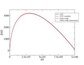
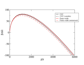
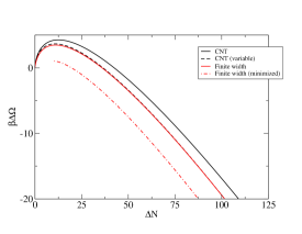
Figure 2: The free energy as a function of cluster size (excess number of molecules in cluster) at $S=1.025,1.175$ and $2.5$ as calculated using the capillary model with fixed $\gamma$, Eq.(39) and Eq.(72), the capillary model with variable $\gamma$ (Eq.(71)), the extended model with fixed width, Eq.(64) and Eq.(68), and the extended model minimized with respect to the width.

Figure 2 shows the energy of formation of a cluster as a function of its size for different values of supersaturation. The figures show the energy as determined using CNT (capillary model with the value of $\gamma=\gamma_{CNT}$ fixed to give the correct surface tension at coexistence ($S=1$), Eq.(72)), the same model but with a supersaturation-dependent value of $\gamma$ (Eq.(71)), the extended model with fixed width and the extended model minimized with respect to the width. It is clear in all cases that the capillary model with fixed $\gamma$ gives lower free energies than when $\gamma$ is allowed to vary and that it is also in closer agreement with the finite-width model. This is somewhat counter intuitive. On the other hand, the extended model with fixed width gives virtually the same results as when the energy is minimized with respect to the width, showing that the simple fixed-width model is adequate. For these reasons, only the capillary model with fixed $\gamma=\gamma_{CNT}$ and the extended model with fixed width will be used below.

V.2 The stationary distribution

The exact stationary distribution is given in Eq.(24). Although both the capillary model and the extended model depend on a single variable, a “radius” denoted $R$ in both cases, the meaning of the parameter is not the same. In order to make a meaningful comparison, we therefore give the stationary distribution using the equimolar radius as the independent variable and noting that

$$\bar{P}(R_{E})=P(R)\frac{dR}{dR_{E}}.$$ (83)

For the capillary model $R=R_{E}$ so that $\bar{P}(R_{E})=P(R)$. For the extended model, we find that

$$\frac{dR_{E}}{dR}=\frac{R^{3}-(max(R-w,0))^{3}}{3wR_{E}^{2}}.$$ (84)

Figure 3 shows the stationary distributions as calculated in CNT and using the extended model for different values of the supersaturation. Also shown are the approximate distribution used to evaluate the nucleation rate. It is apparent that the approximate distribution has the right shape so that it is indeed the case that the stationary distribution is well approximated by the “equilibrium” distribution, $g(X)e^{-\beta\Delta\Omega}$. However, in the case of the extended model, the approximate evaluation of the normalization of the distribution is poor due to the rapidly changing analytic structure of the free energy as a function of cluster radius for small clusters. A surprising result is that the distributions for the capillary model and for the extended model differ even for small supersaturation. This is simply a reflection of the fact that the differences induced by the two models are most pronounced for small clusters. regardless of the supersaturation.

The approximate forms for the nucleation rates given in Eqs.(50) and (76) are not calculated from the exact stationary distribution but, rather, from the approximation given in Eq.(90). The figures show that for CNT this approximation is quite good at low supersaturations but is in considerable error for small clusters. The reason for the increasing error is illustrated in Fig.4 which shows the convergence of the “exact” expression, Eq.(35), as a function of the domain of integration. For large supersaturations, the convergence is slow indicating that larger clusters are contributing significantly to the evaluation of the nucleation rate. For large supersaturations, this calls into question both the monomer attachment picture that underlies CNT and the assumption of non-interacting clusters that is tacitly used in both CNT and the dynamical theory. The main conclusion to be drawn from this result is that even if one could accurately calculate the free energy and distribution of clusters at large supersaturations, it is most likely the case that cluster-cluster interactions would invalidate the assumptions necessary to calculate the nucleation rate, both in CNT and in the general framework described here.

V.3 The nucleation rate

Table 1 gives the nucleation rate as calculated for the two models. For the lowest supersaturation, the extended model gives a much higher nucleation rate. This is almost entirely attributable to the fact that the free energy of the critical cluster is about $10k_{B}T$ lower in the extended model than in the capillary model (and, indeed, the log of the ratio of the nucleation rates is about $9.7$). In all other cases, the nucleation rates of the two models are comparable and similar to that given by the classical CNT formula.

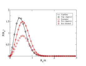
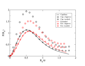
Figure 3: The stationary distribution for $S=1.025$, left panel, and $S=2.5$, right panel. Exact results, i.e. evaluations of Eq.(24) are shown for the capillary and extended models in units such that $\sigma=1$. Also shown is the approximation, Eq.(36), and the approximate distribution scaled so as to have the same maximum as the exact result.

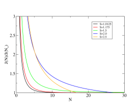
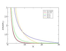
Figure 4: The convergence of $J(N)$, Eq.(35), as a function of $N$ for the capillary model (left panel) and the extended model (right panel) for different values of the supersaturation. Note that in the case of the highest supersaturations, the nucleation rate does not reach a stable value before the integral extends up to the size of the critical cluster, $N_{*}$.

Table 1: Properties of the capillary and extended cluster models as functions of the Supersaturation, $S$. The classical nucleation rate, $J_{CNT}$ is given followed by the critical equimolar radius, $R_{*E}$, the excess mass, $\Delta N_{*}$, and excess free energy, $\Delta\Omega_{*}$, of the critical cluster. Also given are the nucleation rates as calculated from the “exact” expression, Eq.(35), and the approximate expression, Eq.(37), $J$ and $J_{app}$, respectively. Lengths are in units of $\sigma$ and times are in units of $\sigma^{2}/D$.

		Capillary					Extended Model
$S$	$J_{CNT}e^{-\beta\Delta\Omega}$	$R_{*E}$	$\Delta N_{*}$	$\Delta\beta\Omega_{*}$	$\frac{J}{J_{CNT}}$	$\frac{J_{app}}{J_{CNT}}$	$R_{*E}$	$\Delta N_{*}$	$\Delta\beta\Omega_{*}$	$\frac{J}{J_{CNT}}$	$\frac{J_{app}}{J_{CNT}}$
1.025	$1.7\times 10^{-4}$	49.5	300741	3205	0.4	0.37	49.5	300297	3195	6396	5564
1.175	$1.5\times 10^{-3}$	7.8	1149	79	0.84	0.93	7.9	1188	80	0.09	0.11
1.5	$5.7\times 10^{-3}$	3.27	83.6	14.0	1.03	1.45	3.39	92.9	14.9	0.22	0.40
2.0	$1.5\times 10^{-2}$	2.1	21.6	5.9	0.7	1.9	2.2	22.9	5.9	0.5	1.6
2.5	$2.8\times 10^{-2}$	1.8	12.6	4.3	0.9	2.2	1.7	11	3.5	1.1	3.8

VI Conclusions

In this paper an alternative approach to the semi-phenomenological description of nucleation has been presented. The theory is represents a simplification of a description of nucleation based on fluctuating hydrodynamics. One of the advantages of this approach is that there is no ambiguity regarding the choice of reaction coordinate. It also allows for the incorporation of more complex cluster models. When evaluated using the capillary model for a cluster, the results of Classical Nucleation Theory were recovered. A more realistic model that includes a finite interfacial width was also developed. This gives rise to sub-dominant corrections to the free energy of the type described by Prestipino et alPrestipino . It was also shown that the different choices of reaction coordinate give rise to corrections to the free energy that scale logarithmically with the cluster size. When the different models were used to evaluate the nucleation rate, it was found that the dominant effect was the difference in the free energy of the critical cluster in the two models. Thus, despite the fact that the model for the structure of a cluster affects all aspects of the dynamics in our general approach, it is nevertheless the case, as is commonly assumed, that only the correction to the free energy barrier is really important in determining the nucleation rate. This provides post-hoc justification for the combination of the framework of CNT with the use, e.g., of DFT to get better estimates for the free energy barrier.

We also were able to explicitly calculate the stationary distribution. It was shown that the stationary distribution is well approximated, for small clusters, by the “equilibrium” distribution. However, at high supersaturations, it was found that the stationary distribution becomes quite broad and that the nucleation rate becomes dependent on the domain of integration over the cluster sizes. This indicates that the assumption of cluster growth by monomer attachment and detachment is probably invalid as is the assumption of non-interacting clusters. It is therefore the case that quantitative prediction of nucleation rates is not really possible with the theory discussed here. For the conditions considered here, the breakdown occurs when the critical cluster contains between 20 and 100 molecules. A cluster of 100 molecules is still very small and our results illustrate, in some detail, the fact that Classical Nucleation Theory is remarkably robust given the crude assumptions that go into it.

Appendix A Approximate Nucleation Rate

The nucleation rate is

$$J^{-1}=\rho_{\infty}^{-1}D^{-1}\int_{0}^{X_{\ast}}N\left(X\right)g^{1/2}\left(X\right)\exp\left(-\beta\Omega\left(X\right)\right)\left(\int_{X}^{X_{+}}g^{1/2}\left(X^{\prime}\right)\exp\left(\beta\Omega\left(X^{\prime}\right)\right)dX^{\prime}\right)dX$$ (85)

and is the exact expression for the nucleation rate given the assumptions of the theory. In order to develop an approximation it is convenient to switch to the canonical variable so that the nucleation rate becomes

$$J^{-1}=\rho_{\infty}^{-1}D^{-1}\int_{0}^{Y_{\ast}}N\left(Y\right)\left(-\beta\widetilde{\Omega}\left(Y\right)\right)\left(\int_{Y}^{Y_{+}}\exp\left(\beta\widetilde{\Omega}\left(Y^{\prime}\right)\right)dY^{\prime}\right)dY$$ (86)

The first step is to assume that the free energy has a maximum at $Y_{\ast}$ which is defined by

$$\left.\frac{\partial\widetilde{\Omega}\left(Y\right)}{\partial Y}\right|_{Y_{\ast}}=0$$ (87)

so that we can evaluate the inner integral by expanding

$$\exp\left(\beta\widetilde{\Omega}\left(Y^{\prime}\right)\right)\sim\exp\left(\beta\widetilde{\Omega}\left(Y_{\ast}\right)+\frac{1}{2}\beta\widetilde{\Omega}^{\prime\prime}\left(Y_{\ast}\right)\left(Y^{\prime}-Y_{\ast}\right)^{2}\right)$$ (88)

giving

$$J^{-1}\sim\rho_{\infty}^{-1}D^{-1}\exp\left(\beta\widetilde{\Omega}\left(Y_{\ast}\right)\right)\sqrt{\frac{2\pi}{\left|\beta\widetilde{\Omega}^{\prime\prime}\left(Y_{\ast}\right)\right|}}\int_{0}^{Y_{\ast}}N\left(Y\right)\exp\left(-\beta\widetilde{\Omega}\left(Y\right)\right)dY$$ (89)

Before proceeding, note that this is really an approximation to the stationary distribution of

$$\widetilde{P}\left(Y\right)\sim JD^{-1}\exp\left(\beta\widetilde{\Omega}\left(Y_{\ast}\right)\right)\sqrt{\frac{2\pi}{\left|\beta\widetilde{\Omega}^{\prime\prime}\left(Y_{\ast}\right)\right|}}\exp\left(-\beta\widetilde{\Omega}\left(Y\right)\right)$$ (90)

or, in general,

$$P\left(X\right)\sim JD^{-1}\exp\left(\beta\Omega\left(X_{\ast}\right)\right)\sqrt{\frac{2\pi g\left(X\right)g\left(X_{\ast}\right)}{\left|\beta\Omega^{\prime\prime}\left(X_{\ast}\right)\right|}}\exp\left(-\beta\widetilde{\Omega}\left(X\right)\right)$$ (91)

To further simplify, we assume that the free energy has a minimum at $Y=0$ and that $\beta\widetilde{\Omega}\left(Y\right)=aY^{\alpha}+...$ and $N\left(Y\right)=N_{0}Y^{\beta}+...$ for some values of $\alpha,\beta>0$ giving

$$J^{-1} \sim\rho_{\infty}^{-1}D^{-1}\exp\left(\beta\widetilde{\Omega}\left(Y_{\ast}\right)\right)\sqrt{\frac{2\pi}{\left|\beta\widetilde{\Omega}^{\prime\prime}\left(Y_{\ast}\right)\right|}}\int_{0}^{Y_{\ast}}N_{0}Y^{\beta}\exp\left(-aY^{\alpha}\right)dY$$ (92)

$$\sim\rho_{\infty}^{-1}D^{-1}\exp\left(\beta\widetilde{\Omega}\left(Y_{\ast}\right)\right)\sqrt{\frac{2\pi}{\left|\beta\widetilde{\Omega}^{\prime\prime}\left(Y_{\ast}\right)\right|}}N_{0}\frac{1}{\alpha}a^{-\frac{\beta+1}{\alpha}}\int_{0}^{\infty}Z^{\frac{\beta+1-\alpha}{\alpha}}\exp\left(-Z\right)dZ$$

$$=\rho_{\infty}^{-1}D^{-1}\exp\left(\beta\widetilde{\Omega}\left(Y_{\ast}\right)\right)\sqrt{\frac{2\pi}{\left|\beta\widetilde{\Omega}^{\prime\prime}\left(Y_{\ast}\right)\right|}}N_{0}\frac{1}{\alpha}a^{-\frac{\beta+1}{\alpha}}\Gamma\left(\frac{\beta+1}{\alpha}\right)$$

or

$$J\sim D\rho_{\infty}\sqrt{\frac{1}{2\pi}}a^{\frac{1+\beta}{\alpha}}\allowbreak\frac{\alpha}{\Gamma\left(\frac{1+\beta}{\alpha}\right)}\left|\beta\widetilde{\Omega}^{\prime\prime}\left(Y_{\ast}\right)\right|^{1/2}\exp\left(-\beta\widetilde{\Omega}\left(Y_{\ast}\right)\right)$$ (93)

It is easy to translate into the original variables to find

$$J\sim D\rho_{\infty}\sqrt{\frac{1}{2\pi}}\allowbreak a^{\frac{1+\beta}{\alpha}}\allowbreak\frac{\alpha}{\Gamma\left(\frac{1+\beta}{\alpha}\right)}\left|\beta\Omega^{\prime\prime}\left(R_{\ast}\right)g^{-1}\left(R_{\ast}\right)\right|^{1/2}\exp\left(-\beta\Omega\left(R_{\ast}\right)\right).$$ (94)

Appendix B Expansion of the free energy

Beginning with the model expression for the free energy,

$$\Omega\left(R;w\right)-\Omega_{\infty} =\frac{4\pi}{3}\left(R-w\right)^{3}\Delta\omega\left(\rho_{0}\right)$$ (95)

$$+2\pi\left(2\overline{\omega}_{0}w+K\frac{\left(\rho_{0}-\rho_{\infty}\right)^{2}}{w}\right)R^{2}$$

$$-2\pi\left(4\overline{\omega}_{1}w+K\frac{\left(\rho_{0}-\rho_{\infty}\right)^{2}}{w}\right)Rw$$

$$+2\pi\left(2\overline{\omega}_{2}w+\frac{1}{3}K\frac{\left(\rho_{0}-\rho_{\infty}\right)^{2}}{w}\right)w^{2}$$

we minimize by setting the derivative with respect to the width, $w$, equal to zero giving

$$0=-2\left(R-w\right)^{2}\Delta\omega\left(\rho_{0}\right)+\left(2\overline{\omega}_{0}-K\frac{\left(\rho_{0}-\rho_{\infty}\right)^{2}}{w^{2}}\right)R^{2}-8\overline{\omega}_{1}wR+6\overline{\omega}_{2}w^{2}+\frac{1}{3}K\left(\rho_{0}-\rho_{\infty}\right)^{2}$$ (96)

or, after dividing by $R^{3}$ and rearranging,

$$0 =\left(\left(-2\Delta\omega\left(\rho_{0}\right)+2\overline{\omega}_{0}\right)w^{2}-K\left(\rho_{0}-\rho_{\infty}\right)^{2}\right)$$ (97)

$$+\left(4\Delta\omega\left(\rho_{0}\right)-8\overline{\omega}_{1}\right)w^{2}\frac{w}{R}$$

$$+\left(-2\Delta\omega\left(\rho_{0}\right)w^{2}+6\overline{\omega}_{2}w^{2}+\frac{1}{3}K\left(\rho_{0}-\rho_{\infty}\right)^{2}\right)\left(\frac{w}{R}\right)^{2}.$$

We now expand in inverse powers of the radius,

$$w=w_{0}\left(1+a_{1}\frac{w_{0}}{R}+a_{2}\left(\frac{w_{0}}{R}\right)^{2}+...\right)$$ (98)

and solve order by order in $\frac{w_{0}}{R}$ giving

$$w_{0}^{2} =\frac{K\left(\rho_{0}-\rho_{\infty}\right)^{2}}{2\left(-\Delta\omega\left(\rho_{0}\right)+\overline{\omega}_{0}\right)}$$ (99)

$$a_{1} =\frac{\Delta\omega\left(\rho_{0}\right)-2\overline{\omega}_{1}}{\Delta\omega\left(\rho_{0}\right)-\overline{\omega}_{0}}$$

$$a_{2} =\frac{1}{6\left(\Delta\omega\left(\rho_{0}\right)-\overline{\omega}_{0}\right)^{2}}\left(11\left(\Delta\omega\left(\rho_{0}\right)\right)^{2}+\Delta\omega\left(\rho_{0}\right)\left(5\overline{\omega}_{0}-60\overline{\omega}_{1}+9\overline{\omega}_{2}\right)-9\overline{\omega}_{0\overline{\omega}2}-\overline{\omega}_{0}^{2}+60\overline{\omega}_{1}^{2}\right)$$

and

$$\Omega\left(R;w\right)-\Omega_{\infty} =\left(\frac{4}{3}\pi R^{3}\right)\Delta\omega\left(\rho_{0}\right)+\left(4\pi R^{2}\right)\frac{K\left(\rho_{0}-\rho_{\infty}\right)^{2}}{w_{0}}$$ (100)

$$+\left(4\pi R\right)w_{0}^{2}\left(2\Delta\omega\left(\rho_{0}\right)-\overline{\omega}_{0}-2\overline{\omega}_{1}\right)+O\left(R^{0}\right)$$

Of course, we could solve the equation for the width exactly since it is simply a fourth order polynomial in $w$,

$$0 =-K\left(\rho_{0}-\rho_{\infty}\right)^{2}+\left[\frac{K\left(\rho_{0}-\rho_{\infty}\right)^{2}}{3R^{2}}+2\overline{\omega}_{0}-2\Delta\omega\left(\rho_{0}\right)\right]w^{2}$$ (101)

$$+\left[4\frac{\Delta\omega\left(\rho_{0}\right)-2\overline{\omega}_{1}}{R}\right]w^{3}+\left[\frac{6\overline{\omega}_{2}-2\Delta\omega\left(\rho_{0}\right)}{R^{2}}\right]w^{4}.$$

We can also express the free energy in terms of the equimolar radius

$$R_{E} =\left(\frac{1}{4w}\left(R^{4}-(R-w)^{4}\right)\right)^{1/3}=R-\frac{1}{2}w_{0}+\frac{w_{0}}{12}\left(1-6a_{1}\right)\frac{w_{0}}{R}$$ (102)

$$+\frac{w_{0}}{24}\left(4a_{1}-12a_{2}+1\right)\left(\frac{w_{0}}{R}\right)^{2}+O\left(\frac{w_{0}}{R}\right)^{3}$$

we find that

$$R=R_{E}+\frac{w_{0}}{2}+\frac{w_{0}}{12}\left(6a_{1}-1\right)\frac{w_{0}}{R_{E}}+\frac{w_{0}\left(6a_{2}-5a_{1}\right)}{12}\left(\frac{w_{0}}{R_{E}}\right)^{2}+O\left(\left(\frac{w_{0}}{R_{E}}\right)^{3}\right)$$ (103)

giving

$$\Omega\left(R_{E};w\right)-\Omega_{\infty} =\Delta\omega\left(\rho_{0}\right)\allowbreak\left(\frac{4\pi}{3}R_{E}^{3}\right)+w_{0}\left(\frac{K\left(\rho_{0}-\rho_{\infty}\right)^{2}}{w_{0}^{2}}+\frac{\Delta\omega\left(\rho_{0}\right)}{2}\right)\left(4\pi R_{E}^{2}\right)$$ (104)

$$+w_{0}^{2}\left(6\frac{K\left(\rho_{0}-\rho_{\infty}\right)^{2}}{w_{0}^{2}}+\left(13+3a_{1}\right)\Delta\omega-6\overline{\omega}_{0}-12\overline{\omega}_{1}\right)\frac{2\pi}{3}R_{E}\allowbreak+\allowbreak O\left(R^{0}\right)\allowbreak$$

References

• (1) D. Kashchiev, Nucleation : basic theory with applications (Butterworth-Heinemann, Oxford, 2000).
• (2) R. Becker and W. Döring, Annalen der Physik 2416, 719 (1935).
• (3) P. Rien ten Wolde and D. Frenkel, J. Chem. Phys. 109, 9901 (1998).
• (4) D. W. Oxtoby and R. Evans, J. Chem. Phys. 89, 7521 (1988).
• (5) J. F. Lutsko, J. Chem. Phys. 129, 244501 (2008).
• (6) S. Ghosh and S. K. Ghosh, J. Chem. Phys. 134, 024502 (2011).
• (7) A. J. Archer and R. Evans, Molecular Physics 109, 2711 (2011).
• (8) S. Prestipino, A. Laio, and E. Tosatti, Phys. Rev. Lett. 108, 225701 (May 2012).
• (9) W. Lechner, C. Dellago, and P. G. Bolhuis, Phys. Rev. Lett. 106, 085701 (Feb 2011).
• (10) J. F. Lutsko, J. Chem. Phys. 135, 161101 (2011).
• (11) J. F. Lutsko, J. Chem. Phys. 136, 034509 (2012).
• (12) J. F. Lutsko, J. Chem. Phys. 136, 134502 (2012).
• (13) L. Landau and E. Lifshitz, Fluid Mechanics (Pergamon, New York, 1975).
• (14) P.-H. Chavanis, Physica A 387, 5716 (2008).
• (15) C. W. Gardiner, Handbook of Stochastic Methods, 3ed. (Springer, Berlin, 2004).
• (16) P. Hänggi, P. Talkner, and M. Borkovec, Rev. Mod. Phys. 62, 251 (1990).
• (17) E. Lifshitz and L. Pitaevskii, Physical Kinetics: Volume 10 (Course of Theoretical Physics) (Elsevier, Amsterdam, 2010).
• (18) J. S. Langer, Ann. Phys. 54, 258 (1969).
• (19) J. S. Langer and L. A. Turski, Phys. Rev. A 8, 3230 (1973).
• (20) Y. Saito, Statistical Physics of Crystal Growth (World Scientific, Singapore, 1998).
• (21) J. F. Lutsko, J. Chem. Phys. 134, 164501 (2011).