Microscopic resolution of the interplay of Kondo screening and superconducting pairing

Abstract

Magnetic molecules adsorbed on a superconductor give rise to a local competition of Cooper pair and Kondo singlet formation inducing subgap bound states. For Manganese-phthalocyanine molecules on a Pb(111) substrate, scanning tunneling spectroscopy resolves pairs of subgap bound states and two Kondo screening channels. We show in a combined approach of scaling and numerical renormalization group calculations that the intriguing relation between Kondo screening and superconducting pairing is solely determined by the hybridization strength with the substrate. We demonstrate that an effective one-channel Anderson impurity model with a sizable particle-hole asymmetry captures universal and non-universal observations in the system quantitatively. The model parameters and disentanglement of the two screening channels are elucidated by scaling arguments.

I Introduction

Metals become superconducting, when their electrons form singlet Cooper pairs via an attractive interaction. On the other hand, electrons in metals can also undergo another type of singlet formation, namely to form a Kondo screening cloud, when magnetic impurities are present. The fascinating interplay of Cooper pair and Kondo singlet formation Abrikosov and Gorkov (1961); Zittartz and Müller-Hartmann (1970); Zittartz (1970); Müller-Hartmann and Zittartz (1971); Shiba (1973); Matsuura (1979); Sakurai (1970); Balatsky et al. (2006); Kondo (1964); Hewson (1993) can be microscopically observed when magnetic atoms or molecules are adsorbed on superconducting surfaces. The ground state of such a combined system has been predicted to be either a Kondo screened singlet state ($S=0$), if the Kondo scale $k_{\rm B}\,T_{\rm K}$ is much larger than the superconducting pairing energy $\Delta_{\rm sc}$, or an unscreened multiplet state ($S>0$) for $k_{\rm B}\,T_{\rm K}\ll\Delta_{\rm sc}$. Characteristic features include subgap states with bound state energies $E_{b}$ - often called Shiba states. For the singlet ground state with screened impurity spin, the bound states are $S>0$ excitations at $E_{b}<0$, where the Kondo singlet is broken, and for the multiplet ground state the bound states with $E_{b}>0$ are singlet excitations including Kondo screening. When the energy scale for Kondo singlet formation becomes smaller and comparable with the Cooper pairing energy, $k_{\rm B}\,T_{\rm K}\sim\Delta_{\rm sc}$, the bound state energies at $E_{b}$ go to $0$, and the $S>0$ state becomes the ground state. At this point a quantum phase transition (QPT) occurs. The Cooper pair breaking effect is expected to behave like $1-(E_{b}/\Delta_{\rm sc})^{2}$ and thus is most effective here leading to a strong suppression of the superconducting $T_{c}$ for larger impurity concentrations.Müller-Hartmann and Zittartz (1971); Shiba (1973); Balatsky et al. (2006)

For a long time the accurate resolution of the subgap bound states and their dependence on $T_{\rm K}$ and $\Delta_{\rm sc}$ have remained elusive. Recently, the bound states have been analyzed in tunable mesoscopic superconductor-quantum dot-normal lead structures.Deacon et al. (2010) Scanning tunneling microscopy (STM) has been used to detect the local influence of single magnetic atoms on a superconducting substrate.Yazdani et al. (1997) To study the interplay, an experiment with variable magnetic interaction strengths is desirable. Manganese-phthalocyanine (MnPc) molecules on a Pb(111) substrate form a Moire-like superstructure. Tunneling spectroscopy on different Mn sites reveals two Kondo screening channels and pairs of bound states of varying energy $E_{b}$. The large number of different adsorption sites leads to a variety of magnetic interactions and Kondo scales. The smaller Kondo scale lies in the interesting regime $k_{\rm B}\,T_{\rm K}\sim\Delta_{\rm sc}$. Shiba states crossing the Fermi level and the predicted QPT could be observed.Franke et al. (2011) A number of important question remained however unresolved. What is the role of the second Kondo screening channel and does it give rise to a shift of the critical point of the QPT? Which microscopic parameter drives the behavior of the system across the QPT? Does the asymmetry in the STM intensity of the bound states reveal particular physical properties of the system?

Our theoretical approach to address those questions is a combination of scaling arguments and numerical renormalization group (NRG) calculations. Bulla et al. (2008); Satori et al. (1992); Sakai et al. (1993); Yoshioka and Ohashi (2000); Bauer et al. (2007) The former are used to connect the complex experimental situation to an effective Anderson impurity model with one relevant channel and its model parameters. NRG calculations for this model demonstrate that the experimental behavior can be quantitatively understood by only varying the hybridization between MnPc and the substrate. The results are reliable as the NRG is known to capture the Kondo effect accurately in contrast to many other methods, used to describe impurities in superconductors, which contain mean field aspects like classical spins.Zittartz and Müller-Hartmann (1970); Zittartz (1970); Müller-Hartmann and Zittartz (1971); Shiba (1973); Matsuura (1979); Flatté and Byers (1997a, b); Salkola et al. (1997) The accuracy of the theoretical modeling is tested by the direct comparison of the experimental and theoretical results for the point of the QPT and the positions and weights of the bound states.

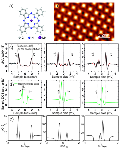
Figure 1: (Color online) a) Molecular structure of Manganese-Phthalocyanine (MnPc), b) Constant-current STM image of highly ordered island of MnPc on Pb(111) (I = 23 pA, $V$ = 100 mV), c) Tunneling spectra taken on different molecules on top of the Mn center (feedback opened at I = 450 pA, $V$ = 8.6 mV). Also shown are the fits used to derive the deconvoluted spectra below in (d). e) Examples of NRG spectra with broadened subgap peaks for similar $E_{b,\alpha}$.

II Experimental results

As detailed in Ref. Franke et al., 2011, the MnPc molecules (see Fig. 1(a)) have been deposited on an atomically clean Pb(111) substrate at room temperature under ultra-high vacuum conditions. STM at 4.5 K resolves highly ordered islands (Fig. 1(b)). Tunneling spectroscopy has been used to resolve the superconducting gap structure and its subgap states, as well as Kondo resonances on different molecules. The superconducting state of the Pb(111) substrate and Pb tip shows as pronounced differential conductance peaks at $E=\pm 2\Delta_{\rm sc}$ with $\Delta_{\rm sc}=1.1$ meV.

Three differential conductance spectra taken on different MnPc molecules are shown in Fig. 1(c). Two larger peaks as well as the two smaller peaks are located at symmetric bias voltages within the gap of the superconductor-superconductor tunneling barrier. The larger peaks are an expression of the Shiba states and indicate the magnetic interaction with the superconducting substrate. The smaller peaks are a result of thermal excitations at the measurement temperature of 4.5 K across the gap. In order to remove the effect of the superconducting tip and finite temperature on the tunneling spectra, we developed a deconvolution method Franke et al. (2011). This procedure consists of extracting the superconducting density of states of the tip from spectra on the bare surface and using the result for fitting the differential conductance spectra of the MnPc spectra assuming a set of Shiba states (for details see Ref. Franke et al., 2011, and the appendix). The result is representative for the quasi-particle density of states (DOS) of the MnPc molecule on the superconducting Pb surface (Fig. 1(d)). From these plots we can deduce the energy of the Shiba states and their intensity. $E_{b,g}$ ($E_{b,s}$) is the energy for the bound state with larger (smaller) weight $w_{b,g}$ ($w_{b,s}$), where $E_{b,g}=-E_{b,s}$. We observe a gradual increase in the asymmetry of the weights when $E_{b,g}$ shifts from negative values to positive ones. This is shown in Fig. 2 as ratio $w_{b,g}/w_{b,s}$.

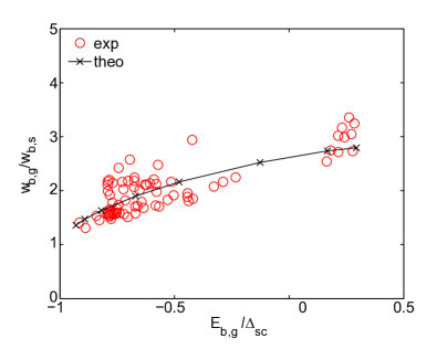
Figure 2: (Color online) Ratio of bound state weights $w_{b,g}/w_{b,s}$ vs bound state energy $E_{b,g}/\Delta_{\rm sc}$. Comparison of experimental results with theory. In all the range of bound state energy we used the model parameters $\varepsilon_{\rm d}/\Delta_{\rm sc}\approx-73$, and $U/\Delta_{\rm sc}\approx 91$ and the overlap $\Gamma$ was varied.

We additionally identify a broad peak at the MnPc center around the Fermi energy (see Fig. 3(b)), which can be fitted by two Fano lineshapes, representing two different Kondo screening processes with $T_{\rm K,2}\gg T_{\rm K,1}$.Franke et al. (2011) $T_{\rm K,2}$ with $\approx 15-45$ meV scales with $T_{\rm K,1}\approx 1-5$ meV (for details the appendix). The occurrence of two Kondo screening channels can be related to the spin state of the MnPc molecule. For the isolated MnPc complex, density functional theory (DFT) calculations have found that the high spin configuration of Mn ($S=5/2$) is reduced to $S=3/2$ and the unpaired electrons occupy the $b_{2g}(d_{xy})$, the $e_{g}(d_{\pi})$, and the $a_{1g}(d_{z^{2}})$ orbital ($x$-axis along an arm of MnPc) and are aligned due to Hund’s rule coupling.Liao et al. (2005) When adsorbed on the Pb surface (in $z$ direction), the $d_{z^{2}}$ orbital hybridizes strongly with the Pb states and is therefore assumed to be quenched.Fu et al. (2007) Hence, the observation of two screening channels suggests a spin state of $S=1$. Since $k_{\rm B}T_{\rm K,2}\gg\Delta_{\rm sc}$, Kondo screening dominates for this channel.Balatsky et al. (2006) Therefore, we only correlate $T_{\rm K,1}\equiv T_{\rm K}\sim\Delta_{\rm sc}$ with the appearance of the bound states inside the gap.

Fig. 3 shows the dependence of $E_{b,\alpha}$ on $R_{\rm K,sc}=k_{\rm B}\,T_{\rm K}/\Delta_{\rm sc}$. At large $R_{\rm K,sc}$, the Kondo screening is efficient and the many-body ground state is a singlet. Here tunneling can occur via the doublet state which involves breaking of the Kondo singlet and rearrangement of Cooper pairs. With decreasing $R_{\rm K,sc}$ this requires less energy and we find $E_{b,\alpha}\to 0$. The level crossing occurs at $R_{\rm K,sc}^{c}\simeq 1.2$. This point can be regarded as the critical point of the QPT and is a universal feature. Further decrease of $R_{\rm K,sc}$ leads to the unscreened doublet ground state.

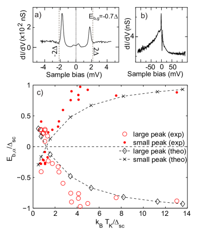
Figure 3: (Color online) a) Tunneling spectrum showing the Shiba states (feedback opened at I = 450 pA, $V$ = 8.6 mV). b) Tunneling spectrum on the same molecule as in (a) in a larger energy scale evidencing a broad background, which can be fitted by two Kondo resonances (feedback opened at I = 470 pA, $V$ = 130 mV). c) Bound state energies $E_{b,\alpha}/\Delta_{\rm sc}$ vs Kondo temperature $T_{\rm K}/\Delta_{\rm sc}$. Comparison of experimental results with theory for the same choice of model parameters as in Fig. 2.

III Theoretical results for the one channel model

For the theoretical description we use an Anderson impurity model (AIM) Hamiltonian of the form

$$H=H_{\rm sc}+H_{d}+H_{\rm mix}.$$ (1)

The superconducting medium reads,

$$H_{\rm sc}\!=\!\!\!\sum_{{\bm{k}},m,{\sigma}}\!\!\!\varepsilon_{{\bm{k}},m}c^{\dagger}_{{\bm{k}},m,\sigma}c_{m,{\bm{k}},\sigma}-\sum_{{\bm{k}},m}(\Delta_{\rm sc}c^{\dagger}_{{\bm{k}},m,\uparrow}c^{\dagger}_{-{\bm{k}},m,\downarrow}+\mathrm{h.c.})$$ (2)

where $c^{\dagger}_{{\bm{k}},m,\sigma}$ creates a band electron with momentum ${\bm{k}}$, spin $\sigma$ and band index $m$, where $m=1,\ldots N_{c}$, and there are $N_{c}$ available channels. $\varepsilon_{{\bm{k}},m}$ is the corresponding electronic dispersion and $\Delta_{\rm sc}$ the gap parameter chosen real. The band electrons hybridize with the impurity states via

$$H_{\rm mix}=\sum_{{\bm{k}},m,{\sigma}}(V_{m}c^{\dagger}_{{\bm{k}},m\sigma}c_{d,m,\sigma}+\mathrm{h.c.}),$$ (3)

where $c^{\dagger}_{d,m,\sigma}$ creates a d-level impurity electron with spin $\sigma$ and index $m=1,\ldots N_{d}$. In the present situation, the number of conduction channels which hybridize is equal to the d-orbital states, i.e. $N_{d}=N_{c}$. We will assume different matrix elements $V_{m}$ due to different overlapping integrals. These matrix elements determine the energy scale for the hybridization of d-states with the substrate through $\Gamma_{m}=\pi V_{m}^{2}\rho_{m,c}$, where $\rho_{m,c}$ is the DOS of the conduction band at the Fermi level $\varepsilon_{\rm F}$. Despite the experimental observation of two Kondo screening channels, we will now show that the behavior of the Shiba states can be well described by a single channel model ($N=1$), suggesting a low energy decoupling of the Kondo channels. For the single channel case the “d-orbital” term $H_{d}$ simply reads,

$$H_{d}=\sum_{{\sigma}}\varepsilon_{d}n_{\sigma}+Un_{\uparrow}n_{\downarrow},$$ (4)

with the d-level position $\varepsilon_{d}$ relative to $\varepsilon_{\rm F}=0$ and the on-site Coulomb interaction with strength $U$, where $n_{\sigma}=c^{\dagger}_{d,\sigma}c_{d,\sigma}$. For this model we perform NRG calculations Bulla et al. (2008) to calculate the lowest energy excitations and their spectral weights, which characterize the subgap bound states. Examples for the low energy spectra can be seen in Fig. 1 (e).

We now explain how to choose the model parameters for the different MnPc molecules on the Pb(111) surface. We expect that the main difference for the MnPc molecules in the different adsorption sites is the magnitude of the hybridization $\Gamma$, which in turn leads to different $T_{\rm K}$. The energy level alignment of the d-states $\varepsilon_{d}$ and Coulomb energy $U$ are, on the contrary, expected to change little with the site.Ji10 We therefore only vary $\Gamma$ to explain the data. The superconducting gap $\Delta_{\rm sc}=1.1$ meV sets the energy scale. The relation of values for $\varepsilon_{d}$, $\Gamma$ and $U$ is constrained to give suitable values for the Kondo temperature $T_{\rm K}\sim\Delta_{\rm sc}$. Their actual value can be fixed by matching the strong experimental weight asymmetry $w_{b,g}/w_{b,s}$ of the Shiba states for the maximal $E_{b,g}>0$ on the doublet side in Fig. 2. This yields $\varepsilon_{d}/\Delta_{\rm sc}\approx-73$, $U/\Delta_{\rm sc}\approx 91$, and $\Gamma/\Delta_{\rm sc}=16$. This corresponds to an asymmetric AIM, with $\xi=\varepsilon_{d}/U+1/2\approx 0.3$. A variation of $\Gamma/\Delta_{\rm sc}$ from $16-46$ then reproduces accurately the weight asymmetry in Fig. 2 on decreasing $E_{b,g}$ and also the variation of $E_{b}^{\alpha}$ with $R_{\rm K,sc}$ in Fig. 3. NRG calculations for an asymmetric one-channel AIM can thus account for the experimentally observed universal features such as $R_{\rm K,sc}^{c}$ and non-universal ones like $w_{b,g}/w_{b,s}$.

Most important for the understanding of the physical processes is the correct description of the QPT. For the one channel non-degenerate AIM and the Kondo model, NRG studies Satori et al. (1992); Sakai et al. (1993); Yoshioka and Ohashi (2000); Bauer et al. (2007) have estimated that the phase transition occurs when $R_{\rm K,sc}^{c}\simeq 0.3$. A deviation from this would indicate that a different number of channels contribute to the Kondo screening of the same electron spin state.žitko et al. (2011) In particular, this may illustrate the role of the second Kondo channel observed in the experiment.

At first sight the experimental result for the QPT, $R_{\rm K,sc}^{c}\simeq 1.2$ (Fig. 3), seems to suggest a more complicated situation than a one-channel model. However, we find that the origin of this discrepancy is the use of different definitions of $T_{\rm K}$, which can vary by a prefactor. In the theoretical works Satori et al. (1992); Sakai et al. (1993); Yoshioka and Ohashi (2000); Bauer et al. (2007) the definition Haldane (1978)

$$T_{\rm K}=0.29[U\Gamma]^{1/2}\mathrm{e}^{\frac{\pi\varepsilon_{\rm d}(\varepsilon_{\rm d}+U)}{2\Gamma U}}$$ (5)

was used. For the experimental values of $T_{\rm K}$, we employ the widely used definition,Goldhaber98 ; Nagaoka02 based on the width of the Kondo resonance $\Delta_{\rm K}$ (half width at half maximum) in the limit $T\to 0$. We adopt the same definition in our NRG calculations ($T_{\rm K}=\Delta_{\rm K}$) and find that $\Delta_{\rm K}$ and the definition in Eq. (5) can differ by a factor 4 (see also Ref. Costi, 2000). Taking this into account our result for the QPT in Fig. 3 is in excellent agreement with the theoretical prediction for a one-channel model. We can thus conclude that the second Kondo screening channel does not shift the transition point.

IV Derivation of the effective model and scaling theory

We now discuss the emergence of the low energy effective one-channel model and its parameters using scaling arguments. First notice that the magnitudes of $\varepsilon_{d}$, $U$ and $\Gamma$ do not correspond to usual atomic values $\sim O(eV)$, but rather to values of the order $100$ meV. This is related to the fact that the AIM under consideration is an effective model valid for low energies. Using insights from the DFT calculations for MnPc,Liao et al. (2005) and the observation of two Kondo channels, we start with a model of the form of equation (1) with the two d-levels coupled to two bands ($N_{c}$$=$$N_{d}$$=$$2$) with the hybridization terms $\Gamma_{1}$$<$$\Gamma_{2}$. Channel 1 thus describes the physical processes related to the smaller Kondo temperature. We assign it to the $d_{xy}$ orbital, since due the spatial orientation the overlap with the substrate is much larger for the $d_{\pi}$ orbital. The impurity term can be written in terms of the level positions $\varepsilon_{d,m}$ relative to $\varepsilon_{\rm F}$, intra orbital Coulomb energy $U_{m}$, inter orbital Coulomb interaction $U_{12}$ and a Hund’s rule interaction $J_{\rm H}$,

$$H_{\rm d} = \sum_{{\sigma},m}\varepsilon_{d,m}c^{\dagger}_{d,m,\sigma}c_{d,m,\sigma}+\sum_{m}U_{m}n_{d,m,\uparrow}n_{d,m,\downarrow}$$

$$+\sum_{\sigma,\sigma^{\prime}}U_{12}n_{d,1,\sigma}n_{d,2,\sigma^{\prime}}-J_{\rm H}\bm{S}_{d,1}\cdot\bm{S}_{d,2},$$

where $S^{\alpha}_{d,m}=\sum_{\sigma_{1},\sigma_{2}}c^{\dagger}_{d,m,\sigma_{1}}\sigma^{\alpha}_{\sigma_{1},\sigma_{2}}c_{d,m,\sigma_{2}}$ with the Pauli matrix $\sigma^{\alpha}$. The complete set of bare parameters of this model can not be extracted from existing DFT calculations,Liao et al. (2005) or experimental observations. Therefore, the following are qualitative arguments on general grounds.

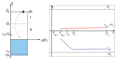
Figure 4: (Color online) Left: Schematic plot of the bare band and impurity energy scales and depiction of two scaling regimes (I,II). Right: Schematic plot of the scaling of the effective level $\varepsilon_{d,1}$ and $\varepsilon_{d,1}+U_{1}$ in the two regimes $\Lambda\in(D_{l},D_{u})$ and $\Lambda\in(T_{\rm K,2},D_{l})$. Scaling stops at $\Lambda\sim T_{\rm K,2}$, and the effective one band model is used to compute the low energy properties.

We now derive scaling equations,Anderson (1970); Haldane (1978) which connect the original model and its parameters at a high energy scale $\Lambda$ of the order of the electronic bandwidth to the low energy effective ones at $\Lambda\sim T_{\rm K,2}$, where the second channel decouples due to its complete Kondo screening. We focus on the quantities in channel 1, where the Shiba states occur. We only include processes with matrix elements $\sim V_{1}^{2}$ explicitly, where the level occupations of $\varepsilon_{d,1}$ changes. There are also contributions $\sim V_{2}^{2}$, whose inclusion leads to quantitative changes in the equations but does not alter the conclusions (for details see the appendix). Band structure calculations Zdetsis et al. (1980) for Pb suggest a situation, where the band $(-D_{l},D_{u})$ is asymmetric with respect to $\varepsilon_{\rm F}$, $D_{l}<D_{u}$. Then, we have two scaling regimes (I, II, see Fig. 4): I, where the scaling process has no counterpart in the occupied states, and II, where the residual band structure is symmetric around $\varepsilon_{\rm F}$. The scaling equations for the energies $\varepsilon_{d,1}$ and $U$ in regime I, i.e., in $\Lambda\in(D_{l},D_{u})$ read,Haldane (1978); Hewson (1993)

$$\frac{d\varepsilon_{d,1}}{d\Lambda} \simeq \frac{\Gamma_{1}}{\pi}\frac{1}{\Lambda-\varepsilon_{d,1}},$$ (7)

$$\frac{dU_{1}}{d\Lambda} \simeq \frac{2\Gamma_{1}}{\pi}\frac{U_{1}}{(\Lambda-\varepsilon_{d,1})(\Lambda-\bar{\varepsilon}_{d,1})},$$ (8)

where $\bar{\varepsilon}_{d,1}=\varepsilon_{d,1}+U_{1}$. Different from the usual approaches we also use a scaling equation for $\Gamma_{1}$, which is derived from $dT_{\rm K,1}/d\Lambda=0$, assuming $T_{\rm K,1}$ as a scaling invariant. Such a scaling procedure can be continued as long as the levels $|\varepsilon_{d,1}|$, $|\varepsilon_{d,1}+U_{1}|$ lie within $(-\Lambda,\Lambda)$ and do not interfere with the Kondo scale. We find $\frac{d\varepsilon_{d,1}}{d\Lambda}>0$ and $\frac{dU_{1}}{d\Lambda}>0$, such that $\varepsilon_{d,1}<0$ is shifting away from $\varepsilon_{F}$ when scaling to lower energy and $U$ decreases. The model becomes more asymmetric in this regime. When $\Lambda\sim D_{l}$, we reach the scaling regime II, with the corresponding scaling equations

$$\frac{d\varepsilon_{d,1}}{d\Lambda} \simeq \frac{\Gamma_{1}}{\pi}\frac{2\varepsilon_{d,1}(\varepsilon_{d,1}+\Lambda)+U_{1}(3\varepsilon_{d,1}-\Lambda)}{(\Lambda^{2}-\varepsilon_{d,1}^{2})(\Lambda+\bar{\varepsilon}_{d,1})},$$ (9)

$$\frac{dU_{1}}{d\Lambda} \simeq \frac{4\Gamma_{1}}{\pi}\frac{\bar{\varepsilon}_{d,1}(\Lambda^{2}-\varepsilon_{d,1}^{2})-\varepsilon_{d,1}(\Lambda^{2}-\bar{\varepsilon}_{d,1}^{2})}{(\Lambda^{2}-\varepsilon_{d,1}^{2})(\Lambda^{2}-\bar{\varepsilon}_{d,1}^{2})}.$$ (10)

For starting values, $\varepsilon_{d,1}(D_{l})<0$, $U_{1}(D_{l})>0$, one has $\frac{d\varepsilon_{d,1}}{d\Lambda}<0$. In this case $\varepsilon_{d,1}$ is shifting towards $\varepsilon_{F}$. Due to the term in the denominator the effect becomes strong when $\Lambda^{2}\sim\varepsilon_{d,1}^{2}$ [see Fig. 4 (right)]. For the same effective starting values we have $\frac{dU_{1}}{d\Lambda}>0$. Hence, $U_{1}$ and ($\varepsilon_{d,1}+U_{1})$ decrease further under the scaling. This scaling can be continued until we reach $\Lambda\sim J_{\rm H}$. We have $D_{l}\sim 3$ eV, and for usual estimates for $J_{\rm H}$ we expect $T_{\rm K,2}<J_{\rm H}<D_{l}$. At this scale the spins lock into the high spin $S=1$ configuration due to the dominating Hund’s coupling. As shown in Ref. Nevidomskyy and Coleman, 2009, this leads to a reduction of the magnetic coupling $J\to J/(2S)$ and the Kondo scale. In our approach it can be included in $\Gamma_{1}$, such that the scaling is slowed down.Nevidomskyy and Coleman (2009) The scaling can then be continued until $\Lambda\sim T_{2,\rm K}$. Then one part of the impurity spin becomes Kondo screened and decouples. At this scale we have an effective single band model with $S=1/2$. Its parameters are substantially reduced from the bare values and generically asymmetric, which clarifies our choice in the earlier NRG calculations. Since NRG calculations for multi-channel models are very challenging, our approach combined with scaling equations could be useful in other situations for complex molecules on surfaces.

In conclusion, we provide a unified experimental and theoretical perspective of the microscopic interplay of Kondo screening and superconducting pairing for MnPc on lead, as manifested in the subgap bound states. We identify the change of hybridization as the relevant quantity and show that in spite of the complex spin state of MnPc and two Kondo screening channels, an effective description based on the one-channel AIM captures both universal aspects like $R_{\rm K,sc}^{c}$ and non-universal ones like the asymmetry of the weights very well. In the future it would be interesting to envisage situations, where different impurity spins can interact, such that different kinds of quantum phase transitions can occur.

Acknowledgment

We wish to thank P. Coleman, M. Haverkort, A.C. Hewson, A. Subedi for helpful discussions and G. Schulze for the deconvolution program of tunneling spectra. JB acknowledges financial support from the DFG through BA 4371/1-1. We also thank the Focus area Nanoscale of Freie Universität Berlin and the Deutsche Forschungsgemeinschaft through Sfb 658 for financial support.

Appendix A Deconvolution procedure

In conventional STM experiments, to first order approximation the $dI/dV$ spectra resemble the density of states of the sample. This relies on a constant density of states of the STM tip. In the presented experiment, the tip is coated with the superconducting material of the substrate, thus exhibiting a Bardeen-Cooper-Schrieffer (BCS) like density of states. To interpret the measured $dI/dV$ spectra as the density of states of the sample, the influence of the tip DOS has to be extracted. We do this by a deconvolution procedure, which has been described and tested in the supplementary material of Ref. Franke et al., 2011.

The STM current $I$ as a function of voltage $V$ has the following form,

$$I(V,\bm{r})\sim\int d\omega\rho_{s}(\omega,\bm{r})\rho_{t}(\omega)[f(\omega)-f(\omega-eV)],$$ (11)

where $\rho_{s}(\omega,\bm{r})$ is the local density of states of the sample at position $\bm{r}$, $\rho_{t}(\omega)$ the one of the tip and $f(\omega)$ is the Fermi function. The deconvolution method consists of a two step process based on fitting the experimental spectra with a simulated density of states. In the first step, the experimental spectrum of the clean surface $\rho_{s}(\omega,\bm{r})=\rho_{s}(\omega)$ is measured and fitted. The density of states of sample and tip are equal, $\rho_{s}(\omega)=\rho_{t}(\omega)$, and follow a BCS density of states broadened by a Lorentzian function. To reproduce the $dI/dV$ spectra, we calculate the tunneling current at each bias voltage and numerically derive the $dI/dV$ function. This function is then fitted to the experimental data to extract the temperature, superconducting gap and broadening. Since the same tip and experimental conditions are used to measure the $dI/dV(V,\bm{r}=\bm{R}_{\rm MnPc})$ spectra on the MnPc molecules, these parameters remain fixed for modeling the tip density of states $\rho_{t}(\omega)$, which is necessary in the next step. The Shiba states are simulated by two Lorentz peaks inside a symmetric gap (modeled by two broadened step functions) around the Fermi level. With this model density of states, the tunneling current is again calculated at each bias voltage and the $dI/dV$ signal derived numerically. The fitting procedure then gives a result for the local $\rho_{s}(\omega,\bm{r}=\bm{R}_{\rm MnPc})$ from which the position, width, and amplitude of the Shiba states can be extracted.

To show the validity and precision of the procedure, we present in Fig. 1c) a direct comparison of the measured and fitted spectra for a number of examples.

Appendix B Definition of the Kondo temperature

For a quantitative comparison between experiment and theory it is important that the same definition of the Kondo temperature $T_{\rm K}$ is used. In the literature one can find different definitions for the Kondo temperature $T_{\rm K}$.Hewson (1993) Theoretically, it is convenient to define it via the magnetic susceptibility of the impurity in the limit $T\to 0$, $\chi_{m}=x/(4T_{\rm K})$ with a suitable prefactor $x$. This quantity is however, not experimentally measured in the present context. The quantity which is most easily accessible experimentally is the width of the Kondo resonance $\Delta_{\rm K}$ (half width at half maximum). To make the comparison of experiment and theory consistent we have used this definition also in the theory, i.e. $\Delta_{\rm K}=T_{\rm K}$. The experimental data is well understood in terms of an overlap of two Fano functions for the two Kondo channels with two different Kondo temperatures $T_{\rm K,1}$, $T_{\rm K,2}$. For details Ref. Franke et al., 2011 can be consulted. In Table 1 we display a number of values found on different molecules.

$E_{b,g}/\Delta_{\rm sc}$	$T_{\rm K,1}$ (K)	$T_{\rm K,2}$ (K)
-0.76	52$\pm$5	480$\pm$60
-0.69	53$\pm$8	330$\pm$40
-0.46	38$\pm$2	280$\pm$50
-0.29	29$\pm$5	420$\pm$ 30
0.24	14$\pm$10	210$\pm$ 50

Table 1: Exemplary values for $T_{\rm K,1}$ and $T_{\rm K,2}$ on different molecules with energy of the larger Shiba state $E_{b,g}/\Delta_{\rm sc}$.

Appendix C Scaling equations for the two channel model

Here we present the complete set of scaling equations for the two-channel model. We will argue that the conclusions in the main text are not changed qualitatively due to additional terms proportional to $V_{2}^{2}$. The starting point is the effective two orbital model in equation (1) together with (IV). In the following we focus on the complete scaling equations in regime II. The scaling equations in regime I only contain a part of the terms and show how the asymmetry is increased for an asymmetric band. They can be derived and discussed in a similar fashion. For each orbital there are 4 possible states, such that there are 16 atomic states which can be described by the occupation numbers $n_{1,\sigma}$, $n_{2,\sigma}$ for orbital 1 and 2, respectively. Due to the Hund’s rule term ($J_{\rm H}>0$),

$$H_{H}=-J_{\rm H}\bm{S}_{d,1}\cdot\bm{S}_{d,2},$$ (12)

the atomic eigenbasis for the singly occupied situation, $n_{1,\sigma}=n_{2,\sigma}=1$ is given by singlet and triplet states, $\!|S,S_{z}\ \!\!\rangle$, and hence we use those quantum numbers, where $S$ is the total spin with $z$-component $S_{z}$. One has

$$H_{H}\!|1,S_{z}\ \!\!\rangle=-J_{\rm H}\!|1,S_{z}\ \!\!\rangle,\;\;H_{H}\!|0,S_{z}\ \!\!\rangle=3J_{\rm H}\!|0,S_{z}\ \!\!\rangle,$$ (13)

i.e., the triplet state state has the lowest energy, and the energy difference is $4J_{\rm H}$ for our definition of $\bm{S}_{d,i}$, which does not include a factor $1/2$. For the derivation of the scaling equations it is useful to define Hubbard operators $X_{ab}=\!|a\ \!\!\rangle\langle\!b\ \!|$ for the atomic states.Hewson (1993) The atomic terms can be given in diagonal energy representation with $E_{n_{1,\sigma},n_{2,\sigma}}$ and $\bar{E}_{S,S_{z}}$. The hybridization term constitutes of a lengthy expression in terms of those Hubbard operators taking into account all possible processes of different occupation. The single particle occupation parameters of the Hamiltonian can be expressed as $\varepsilon_{d,1,\sigma}=E_{n_{1,\sigma}=1,0}-E_{0,0}$. By projecting out high energetic particle and hole states in the bath Hewson (1993) we find the equations,

$$\frac{d\varepsilon_{d,1}}{d\Lambda} = \frac{\Gamma_{1}}{\pi}\Big{[}\frac{1}{\Lambda-\varepsilon_{d,1}}+\frac{1}{\Lambda+\varepsilon_{d,1}+U_{1}}-\frac{2}{\Lambda+\varepsilon_{d,1}}\Big{]}$$

$$+ \frac{\Gamma_{2}}{\pi}\Big{[}\frac{3/2}{\Lambda+\varepsilon_{d,2}+U_{12}-J_{\rm H}}+\frac{1/2}{\Lambda+\varepsilon_{d,2}+U_{12}+3J_{\rm H}}-\frac{2}{\Lambda+\varepsilon_{d,2}}\Big{]},$$

$$\frac{dU_{1}}{d\Lambda} = \frac{2\Gamma_{1}}{\pi}\Big{[}\frac{1}{\Lambda+\varepsilon_{d,1}}-\frac{1}{\Lambda-\varepsilon_{d,1}}+\frac{1}{\Lambda-\varepsilon_{d,1}-U_{1}}-\frac{1}{\Lambda+\varepsilon_{d,1}+U_{1}}\Big{]}$$

$$+ \frac{\Gamma_{2}}{\pi}\Big{[}\frac{2}{\Lambda+\varepsilon_{d,2}+2U_{12}}-\frac{3}{\Lambda+\varepsilon_{d,2}+U_{12}-J_{\rm H}}-\frac{1}{\Lambda+\varepsilon_{d,2}+U_{12}+3J_{\rm H}}+\frac{2}{\Lambda+\varepsilon_{d,2}}\Big{]}.$$

Similar equations are found for $\varepsilon_{d,2}$ and $U_{2}$, where one has to interchange the indices $\alpha=1,2$ in $\varepsilon_{d,\alpha}$, $\Gamma_{\alpha}$ and $U_{\alpha}$ on the right hand side. An equation for $J_{\rm H}$ follows from $4J_{\rm H}=\bar{E}_{S=0,S_{z}=0}-\bar{E}_{S=1,S_{z}=1}$,

$$\frac{dJ_{\rm H}}{d\Lambda} = \sum_{m=1}^{2}\frac{\Gamma_{m}}{4\pi}\Big{[}\frac{1}{\Lambda-(\varepsilon_{d,m}+U_{12}+3J_{\rm H})}+\frac{1}{\Lambda+\varepsilon_{d,m}+U_{12}+U_{1}-3J_{\rm H}}$$

$$-\frac{1}{\Lambda-(\varepsilon_{d,m}+U_{12}-J_{\rm H})}-\frac{1}{\Lambda+\varepsilon_{d,m}+U_{12}+U_{1}+J_{\rm H}}\Big{]}.$$

We can represents $U_{12}$ as $U_{12}=\bar{E}_{S=1,S_{z}=1}-E_{0,0}-\varepsilon_{d,1}-\varepsilon_{d,2}+J_{\rm H}$, and find

$$\frac{dU_{12}}{d\Lambda} = \sum_{m=1}^{2}\frac{\Gamma_{m}}{\pi}\Big{[}\frac{3/4}{\Lambda-(\varepsilon_{d,m}+U_{12}-J_{\rm H})}+\frac{3/4}{\Lambda+\varepsilon_{d,m}+U_{12}+U_{m}+J_{\rm H}}+\frac{1/4}{\Lambda-(\varepsilon_{d,m}+U_{12}+3J_{\rm H})}$$

$$+\frac{1/4}{\Lambda+\varepsilon_{d,m}+U_{12}+U_{m}-3J_{\rm H}}-\frac{3/2}{\Lambda+\varepsilon_{d,m}+U_{12}-J_{\rm H}}-\frac{1/2}{\Lambda+\varepsilon_{d,m}+U_{12}+J_{\rm H}}$$

$$-\frac{1}{\Lambda+\varepsilon_{d,m}+U_{m}}-\frac{1}{\Lambda-\varepsilon_{d,m}}+\frac{2}{\Lambda+\varepsilon_{d,m}}\Big{]}.$$

We can use the Kondo scales in the two channels $T_{{\rm K},m}$ as scaling invariants. There is an approximate form $T_{{\rm K},m}\simeq T_{{\rm K},m}^{0}\exp(-\alpha J_{\rm H})$ for the situation with Hund’s rule coupling,Nishikawa, Y. and Crow, D. J. G. and Hewson, A. C (1997b) where $T_{{\rm K},m}^{0}$ is the Kondo scale for $J_{\rm H}=0$. From this we can also derive scaling equations for $\Gamma_{m}$. If one neglects $J_{\rm H}$ in the denominator as being smaller than the other scales then one finds $dJ_{\rm H}/d\Lambda\simeq 0$, such that the Hund’s coupling varies little.Nevidomskyy and Coleman (2009)

The Eqs. (9) and (10) in the main text for regime II correspond to (C), (C) without the terms proportional to $\Gamma_{2}$. In order to have Kondo physics in both channels, we need the atomic ground state to be one where both orbitals are singly occupied, which implies $\varepsilon_{d,m}+U_{12}<0$ and $\varepsilon_{d,m}+U_{12}+U_{m}>0$. We also expect a deviation from particle-hole symmetry $\varepsilon_{d,m}=-U_{12}-U_{m}/2$. In the main text we have argued that from the term proportional to $\Gamma_{1}$ one finds $\frac{d\varepsilon_{d,1}}{d\Lambda}<0$. It is easy to see that for $\Lambda+\varepsilon_{d,2}>0$, $\Lambda+\varepsilon_{d,2}+U_{12}-J_{\rm H}>0$ and $\Lambda+\varepsilon_{d,2}+U_{12}-J_{\rm H}>0$ the term proportional to $\Gamma_{2}$ is also negative, such that $\frac{d\varepsilon_{d,1}}{d\Lambda}<0$ is reinforced. Similarly, the additional term $\sim\Gamma_{2}$ in Eq. (C) has the same sign as the first term and therefore $\frac{dU_{1}}{d\Lambda}>0$ is maintained. Hence, the qualitative picture remains unchanged, when these additional terms are taken into account. There will however be quantitative changes in the scaling. The quantities in channel 2, $\varepsilon_{d,2}$, $U_{2}$ possess a similar scaling flow, but are not of major interest here as the corresponding Kondo temperature $T_{\rm K,2}$ largely exceeds the superconducting gap. A more complete discussion of the different regimes of the scaling equations and the different resulting behavior is beyond the scope of this work, but can be subject of a separate study.

References

- Abrikosov and Gorkov (1961) A. A. Abrikosov and L. P. Gorkov, Sov. Phys. JETP 12, 1243 (1961).
- Zittartz and Müller-Hartmann (1970) J. Zittartz and E. Müller-Hartmann, Z. Physik. 232, 11 (1970).
- Zittartz (1970) J. Zittartz, Z. Physik. 237, 419 (1970).
- Müller-Hartmann and Zittartz (1971) E. Müller-Hartmann and J. Zittartz, Phys. Rev. Lett. 26, 428 (1971).
- Shiba (1973) H. Shiba, Prog. Theor. Phys 50, 50 (1973).
- Matsuura (1979) T. Matsuura, Prog. Theor. Phys. 57, 1823 (1979).
- Balatsky et al. (2006) A. V. Balatsky, I. Vekhter, and J.-X. Zhu, Rev. Mod. Phys. 78, 373 (2006).
- Kondo (1964) J. Kondo, Prog. Theor. Phys 32, 37 (1964).
- Hewson (1993) A. C. Hewson, The Kondo Problem to Heavy Fermions (Cambridge University Press, Cambridge, 1993).
- Sakurai (1970) A. Sakurai, Prog. Theor. Phys. 44, 1472 (1970).
- Deacon et al. (2010) R. S. Deacon, Y. Tanaka, A. Oiwa, R. Sakano, K. Yoshida, K. Shibata, K. Hirakawa, and S. Tarucha, Phys. Rev. Lett. 104, 076805 (2010).
- Yazdani et al. (1997) A. Yazdani, B. A. Jones, C. P. Lutz, M. F. Crommie, and D. M. Eigler, Science 275, 1767 (1997).
- Franke et al. (2011) K. J. Franke, G. Schulze, and J. I. Pascual, Science 332, 940 (2011).
- Bulla et al. (2008) R. Bulla, T. Costi, and T. Pruschke, Rev. Mod. Phys. 80, 395 (2008).
- Satori et al. (1992) K. Satori, H. Shiba, O. Sakai, and Y. Shimizu, J. Phys. Soc. Japan 61, 3239 (1992).
- Sakai et al. (1993) O. Sakai, Y. Shimizu, H. Shiba, and K. Satori, J. Phys. Soc. Japan 62, 3181 (1993).
- Yoshioka and Ohashi (2000) T. Yoshioka and Y. Ohashi, J. Phys. Soc. Japan 69, 1812 (2000).
- Bauer et al. (2007) J. Bauer, A. Oguri, and A. Hewson, J. Phys.: Cond. Mat. 19, 486211 (2007).
- Flatté and Byers (1997a) M. E. Flatté and J. M. Byers, Phys. Rev. Lett. 78, 3761 (1997a).
- Flatté and Byers (1997b) M. E. Flatté and J. M. Byers, Phys. Rev. B 56, 11213 (1997b).
- Salkola et al. (1997) M. I. Salkola, A. V. Balatsky, and J. R. Schrieffer, Phys. Rev. B 55, 12648 (1997).
- Liao et al. (2005) M.-S. Liao, J. D. Watts, and M.-J. Huang, Inorganic Chemistry 44, 1941 (2005).
- Fu et al. (2007) Y.-S. Fu, S.-H. Ji, X. Chen, X.-C. Ma, R. Wu, C.-C. Wang, W.-H. Duan, X.-H. Qiu, B. Sun, P. Zhang, et al., Phys. Rev. Lett. 99, 256601 (2007).
- (24) S.-H. Ji, et al., Chin. Phys. Lett. 27, 087202 (2010).
- Haldane (1978) F. D. M. Haldane, Phys. Rev. Lett. 40, 416 (1978).
- (26) D. Goldhaber-Gordon, et al., Phys. Rev. Lett. 81, 5225 (1998).
- (27) K. Nagaoka, et al., Phys. Rev. Lett. 88, 077205 (2002).
- Costi (2000) T. A. Costi, Phys. Rev. Lett. 85, 1504 (2000).
- žitko et al. (2011) R. žitko, O. Bodensiek, and T. Pruschke, Phys. Rev. B 83, 054512 (2011).
- Anderson (1970) P. W. Anderson, J. Phys. C 3, 2435 (1970).
- Zdetsis et al. (1980) A. D. Zdetsis, E. N. Economou, and D. A. Papaconstantopoulos, Journal of Physics F: Metal Physics 10, 1149 (1980).
- Nevidomskyy and Coleman (2009) A. H. Nevidomskyy and P. Coleman, Phys. Rev. Lett. 103, 147205 (2009).
- Nishikawa, Y. and Crow, D. J. G. and Hewson, A. C (1997b) Y. Nishikawa, D. J. G. Crow, and A. C. Hewson Phys. Rev. B 82, 115123 (2010b).