Genealogies of rapidly adapting populations

Abstract

The genetic diversity of a species is shaped by its recent evolutionary history and can be used to infer demographic events or selective sweeps. Most inference methods are based on the null hypothesis that natural selection is a weak or infrequent evolutionary force. However, many species, particularly pathogens, are under continuous pressure to adapt in response to changing environments. A statistical framework for inference from diversity data of such populations is currently lacking. Toward this goal, we explore the properties of genealogies in a model of continual adaptation in asexual populations. We show that lineages trace back to a small pool of highly fit ancestors, in which almost simultaneous coalescence of more than two lineages frequently occurs. While such multiple mergers are unlikely under the neutral coalescent, they create a unique genetic footprint in adapting populations. The site frequency spectrum of derived neutral alleles, for example, is non-monotonic and has a peak at high frequencies, whereas Tajima’s $D$ becomes more and more negative with increasing sample size. Since multiple merger coalescents emerge in many models of rapid adaptation, we argue that they should be considered as a null-model for adapting populations.

Evolutionary change is usually too slow to be observed in real time. A sequence sample represents a static snapshot from which we want to learn about a dynamic evolutionary process. The predominant framework to analyze such population genetic data and infer demographic history is Kingman’s neutral coalescent. Within this model, all individuals are equivalent, i.e., there are no fitness differences, and pairs of lineages merge at random. The statistical properties of genealogies in this simple population genetic model can be computed exactly Kingman:1982p28911 ; Derrida:1991p1707 , facilitating comparison to data. One central prediction of the neutral coalescent is that the genetic diversity of a population is proportional to its size. This prediction, however, is at odds with the observed weak correlation between genetic diversity and population size, a paradox often remedied by the definition of an effective population size via the genetic diversity. The model has been generalized to account for historic changes in population size, mutation rates, geographical structure and the effects of purifying selection Nordborg:1997p43854 ; Charlesworth:1993p36005 ; Walczak:2011p45228 ; Ofallon:2010p43263 ; Barton:2004p34826 . Positive selection, however, has proved difficult to incorporate, and progress has been limited to rare selective sweeps Barton:1998p28270 ; Durrett:2005p40919 and weak selection Krone:1997p19666 .

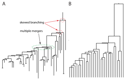
In many populations, particularly large microbial populations, selection is neither rare nor weak. Instead, these populations are under sustained pressure to adapt to changing environments. Prominent examples include pathogens like influenza that continuously evade human immune responses or HIV, which establishes a chronic infection despite heavy immune predation. The genealogical trees reconstructed from sequence samples often suggest substantial departure from neutrality; see Bedford:2011p47600 for examples from viral evolution or Seger:2010p39561 for eukaryotic examples. The influenza tree shown in Fig. 1, for instance, is incompatible with a neutral genealogy, since there are parts where many lineages merge in a very brief period, and the tree often branches extremely unevenly with very few individuals on one branch and many on the other. These two observations represent fundamental deviations from the standard neutral model, even when a varying population size is allowed. Strelkowa and Lässig present a detailed analysis of Influenza A evolution and conclude that influenza is governed by coalescence processes different from the Kingman coalescent Strelkowa:2012p48466 .

To analyze and interpret genealogies of populations under sustained directional selection, an alternative simple null model would be extremely useful. The features of genealogies discussed above are in fact common to a class of non-Kingman coalescence models, which have received considerable attention in the mathematical coalescent literature Pitman:1999p41045 ; Berestycki:2009p45808 . A special case is the Bolthausen-Sznitman coalescent (BSC) Bolthausen:1998p47390 , which has been shown to describe the genealogies in models where a population expands into uninhabited territory Brunet:2007p18866 . On the basis of a particular exact solution and a phenomenological theory, Brunet et al. conjectured that genealogies in all models of the same universality class (the class of stochastic Fisher-Kolmogorov-Petrovskii-Piscounov (FKPP) waves Fisher:1937p47380 ; Kolmogorov:1937p47381 ) are described by the BSC; see Brunet:2012p45985 for a recent review. This universality class contains all models with short range dispersal and logistic growth with constant rate in partially filled demes.

We will argue in this article that the BSC emerges generically in models of rapidly adapting asexual populations in a similar way as it describes genealogies in traveling waves of FKPP type. We present extensive computer simulations and investigate the distribution of heterozygosity in the population, the average time to the most recent common ancestor, and the site frequency spectrum (SFS). Most notably, the SFS is non-monotonic with a large number of high frequency derived alleles. We then study a simplified model analytically and show that the underlying genealogical process is approximately the BSC. In the discussion, we outline the basic features of the BSC and discuss its applicability to wider classes of models.

Figure 1: Panel A shows a maximum-likelihood tree of influenza nucleotide sequences (HA segment) sampled in Asia in 2009 (subtype H3N2) produced using Fasttree Price:2009p47657 . Panel B shows a tree drawn from a simulation of our model of adapting populations. Both trees often branch very unevenly with almost all descendants on the left-most branch. While approximate multiple mergers are common in both trees, the influenza tree does not display the uniformly long terminal branches we observe in simulations. This could be due to heterogeneous sampling of influenza. Trees are drawn with Figtree http://tree.bio.ed.ac.uk/software/figtree/.

I The model

The evolutionary dynamics of a large population are mainly determined by the distribution of fitness in the population. In general, fitness depends on many traits, which are affected by mutations. In a rapidly changing environment, populations are far from any fitness optimum, with many mutations available that increase fitness (and even more that decrease fitness).

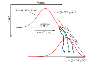
To model such scenarios, we consider a collection of $N$ asexual individuals that are characterized by a log-fitness $y$, which determines their average reproductive success. Specifically, the number offspring of an individual is Poisson distributed with mean $\exp(y-\lambda)$, where $\lambda=\bar{y}-1+N/N_{0}$ keeps the population size roughly at $N_{0}$. The log-fitness of individuals is changed by mutation with probability $\mu$ per generation, where the mutational effect, $\delta$, is drawn from a distribution $K(\delta)$. The balance between frequent mutation and selection results in a population that behaves as a traveling pulse along the fitness axis with a steady fitness variance $\sigma^{2}$; see Fig. 2. Absolute fitness itself is of course not increasing indefinitely, but increasing fitness is offset by environmental deterioration and deleterious mutations.

We have implemented this model as a computer program (see SI) that allows for different mutation distributions $K(\delta)$. In addition, the program keeps track of the parents of each new individual and thereby saves the complete genealogy of the population. Individuals not leaving any offspring are removed from the genealogical record. From this genealogical record, quantities like pair coalescence times are readily obtained. Furthermore, we can calculate site frequency spectra of neutral mutations by integrating over all positions in the genealogies where such mutations might have occurred.

Similar models have been used by a number of authors Tsimring:1996p19688 ; Desai:2007p954 ; Rouzine:2003p33590 ; Neher:2010p30641 ; Hallatschek:2011p39697 ; Park:2007p4335 who have studied the rate of adaptation in these models. Here, we focus on genealogies and their relation to observed genetic diversity. If mutations are frequent relative to the typical effect size of mutations, the model has a continuous time limit described by a stochastic differential equation for the distribution $c(y,t)$ of log-fitness $y$ in the population Cohen:2005p45154 ; Good:2012p47545 ; Hallatschek:2011p39697

$$\partial_{t}c(y,t)=D\partial_{y}^{2}c(y,t)-\Delta_{\mu}\partial_{y}c(y,t)+(y-\lambda)c(y,t)+\mathrm{drift}\ ,$$ (1)

where the last term represents the stochastic nature of reproduction; see SI for derivation. The diffusion constant and the average mutation input are given by $D=\mu\langle\delta^{2}\rangle/2$ and $\Delta_{\mu}=\mu\langle\delta\rangle$, respectively, where the average $\langle\ldots\rangle$ is over the distribution of mutational effects $K(\delta)$. The exact form of the distribution of mutational effects and the relative importance of deleterious and beneficial mutations are irrelevant as long as this diffusive approximation is valid (see SI). Unless otherwise stated, we use $\mu=1$ and draw mutational effects from a Gaussian distribution with variance $s^{2}$ and zero mean.

In this model, large populations attain a steady fitness distribution of roughly Gaussian shape with variance $\sigma^{2}\approx D^{2\over 3}(24\log\tilde{N})^{1\over 3}$, where $\tilde{N}=ND^{1\over 3}$ Tsimring:1996p19688 ; Cohen:2005p45154 . The distribution translates towards higher fitness with a velocity $v=\sigma^{2}+\Delta_{\mu}$. The distribution and its landmarks are sketched in Fig. 2. It is convenient to measure log-fitness relative to the population mean, $x=y-\bar{y}$. The fittest individuals of the population reside roughly $x_{c}\approx\sigma^{4}/4D$ above the population mean. Computer programs and analysis scripts are available on the author’s website.

Figure 2: Ancestral lineages in evolving populations. The figure shows the fitness distribution of the population, translating towards higher fitness with velocity $\sigma^{2}+\Delta_{\mu}$, at two time points. Randomly sampled individuals (green, blue, and violet dots in the later population) tend to come from the center of the distribution, while ancestors tend to be among the fittest in the population. The ancestral lineages wiggle due to mutations that randomly perturb their fitness. Simultaneously, lineages move towards the high fitness edge, where they are likely to meet and coalesce. The fittest individuals are typically at $x_{c}\approx\sigma^{4}/4D$ above the mean fitness.

II Results

We first present simulation results of our model and contrast the patterns of genetic diversity of continuously adapting populations with neutral expectations. Below, we will analyze our model mathematically and show that the striking differences result from the exponential amplification of individual lineages by selection.

II.1 Distribution of heterozygosity and pair coalescence times

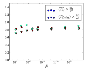
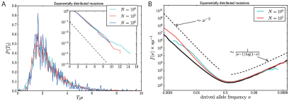
Assuming a molecular clock, the expected number of neutral differences between two genomes is $\pi=2T_{2}\mu_{n}$, where $\mu_{n}$ is the neutral mutation rate and $T_{2}$ is the time to the most recent ancestor of the pair of sequences. Across many realizations of the process (e.g. independent loci), $T_{2}$ follows a distribution $P(T_{2})$, which in the neutral case is exponential with mean $N$. Simulation results for our model shown in Fig. 3 display a very different distribution of $T_{2}$ and equivalently $\pi$. Very few pairs of sequences coalesce early, which results in the long terminal branches observed in trees; see Fig. 1B. We then observe a peak in coalescence around $t\approx\sigma^{2}/2D$, after which the distribution of pair coalescence times decays exponentially with a characteristic time constant proportional to $\sigma^{2}/2D$. Within a neutral coalescent framework, a distribution of this kind would be interpreted as a rapid population expansion starting $\sigma^{2}/2D$ in the past. Prior to this expansion, the population size would be estimated to have been constant at $N_{e}\propto\sigma^{2}/2D$. However, the size of the population did not change in our model. Instead, the population was adapting by many small steps, and the conclusion that $N$ increased in the past is wrong.

Figure 3: The distribution of pair coalescence times (proportional to heterozygosity) in a model of rapidly adapting populations. After rescaling time by $\sigma^{2}/2D$ curves for different $N$ and $s$ collapse onto a single master curve. This collapse demonstrates that $\sigma^{2}/2D\propto D^{-{1\over 3}}(\log\tilde{N})^{1\over 3}$ is the time scale of coalescence. Following a delay $T_{delay}\approx\sigma^{2}/2D$, $T_{2}$ is exponentially distributed, as is apparent from the inset showing the cumulative distribution $P(T_{2}>T)$. An exponential $\exp[-2TD/\sigma^{2}]$ is indicated as a black dashed line. Different line styles correspond to $s=0.01$ (solid), $s=0.001$ (dashed), and $s=0.0001$ (dotted), while the mutation rate is $\mu=1$. For each parameter combination, random pairs are sampled at 10000 time points $2s^{-2/3}$ generations apart.

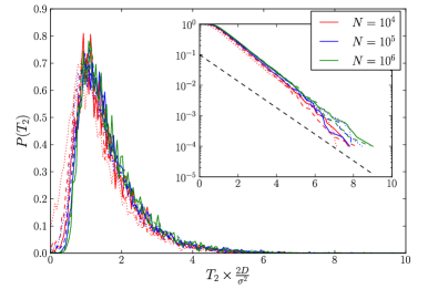
Two lineages chosen at random from the population are most likely from near the center of the fitness distribution. There are many individuals in this part of the distribution, so the probability of immediate coalescence is therefore low. While the sampled individuals are typical, their ancestors tend to have higher than average fitness. Only after ancestral lineages have moved to the high fitness tail of the distribution, where only few individuals are, does the rate of coalescence become appreciable. This migration of lineages towards higher fitness is a well known effect Hermisson:2002p47231 ; Ofallon:2010p43263 ; Rouzine:2007p17401 and illustrated in Fig. 2. The speed at which lineages move toward higher (relative) fitness is initially $\sigma^{2}$ (the speed of the mean minus the mutational input), while they slow down as they reach the tip. Consistent with the above interpretation, the delay of coalescence, $T_{delay}$, is roughly twice the time required for the mean fitness to catch up with the high fitness nose, i.e., $T_{delay}\approx 2x_{c}\sigma^{-2}=\sigma^{2}/2D$. After lineages have moved to the high fitness tail, they seem to coalesce uniformly with a time constant $T_{c}\approx\sigma^{2}/2D$. From the dependence of $\sigma^{2}$ on population parameters, we see that $T_{c}\propto(\log\tilde{N})^{1\over 3}$ increases only weakly with the population size.

II.2 Site frequency spectra

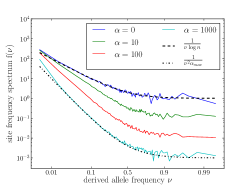
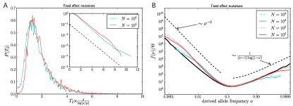
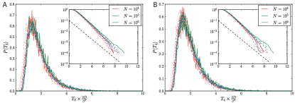
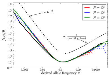
The density $f(\nu)d\nu$ of neutral derived alleles in the frequency interval $[\nu,\nu+d\nu]$ is known as the site frequency spectrum (SFS). The neutral SFS is a convenient summary of the neutral diversity segregating in the population. A mutation that happened on a particular branch of the genealogy will later be present in all individuals that descend from this branch. Hence the SFS harbors information about the distribution of branch weights and the branch length of the genealogy. In Kingman’s coalescent, the SFS is simply given by $f(\nu)=\Theta/\nu$, where $\Theta=2\langle T_{2}\rangle\mu$ is the average heterozygosity. Importantly, it is a monotonically decreasing function of the frequency. Fig. 4 shows site frequency spectra measured in simulations of our model. The most striking qualitative difference is the non-monotonicity, a feature known to be common in the presence of selective sweeps due to hitch-hiking Fay:2000p35077 .

The non-monotonicity of $f(\nu)$ implies the existence of long branches deep in the tree that are ancestors of almost everybody in the population, whereas a small minority of the population descends from different lineages. Such very asymmetric branchings are unlikely in Kingman’s coalescent, where at any split the fraction of individuals that go left or right is uniformly distributed Derrida:1991p1707 . Such asymmetric branchings are common in our model and frequently observed in reconstructed genealogies from rapidly adapting organisms; see Fig. 1A.

The axes in Fig. 4 are scaled to facilitate the comparison to analytic results. At low frequencies, the site frequency spectrum is proportional to $\nu^{-2}$ Basdevant:2008p45781 ; Neher:2011p42539 and therefore much steeper than the neutral SFS in Kingman’s coalescent, $f(\nu)\propto\nu^{-1}$. Hence samples will be dominated by singletons. In addition, $f(\nu)$, is non-monotonic and increases as $\nu\to 1$.

The majority of the contributions to the increase of $f(\nu)$ for $\nu\to 1$ stem from the very last coalescent event. In this last coalescent event, two or more lineages are merging. One of these lineages is typically the ancestor of almost the entire sample, while the others share the remaining minority. The distribution of the offspring of these lineages and their number has been studied by Goldschmidt and Martin Goldschmidt:2005p47276 , who showed that the distribution of the size of the biggest lineage is asymptotically $\propto(1-\nu)^{-1}$. In the SI (section 3), we derive the more accurate approximation

$$f(\nu)\approx\frac{T_{c}\mu}{(\nu-1)\log(1-\nu)}\qquad 1-\nu\ll 1\ .$$ (2)

To compare the SFS of our model to that of the BSC across the entire range of $\nu$, we simulated the idealized BSC and find very good agreement (solid black line in Fig. 4). The SFS of the idealized BSC deviates from that of the model of adaptation only at very low allele frequencies. The model of adaptation tends to have even more rare alleles than the BSC, which is due to the fact that lineages have to move to the high fitness tail before coalescence sets in.

The non-monotonicity $f(\nu)$ is a clear indication that the genealogies in this model with selection are fundamentally different from canonical neutral genealogies (Kingman). In Kingman’s coalescent, neither constant or exponentially growing population sizes give rise to non-monotonic SFS; see supplementary Fig. 8.

Figure 4: Site frequency spectrum of (derived) neutral alleles in rapidly adapting populations is non-monotonic with peaks at low frequencies and near fixation. The asymptotic behavior of the SFS at low and high derived frequencies is shown as dashed black lines. The solid black line is the SFS of the BSC simulated using Eqs. (7) and (8) with $N=100000$ and averaged over 10000 runs. Line styles and parameters are as in Fig. 3.

II.3 The time to the MRCA

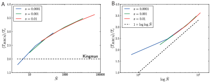
In Kingman’s coalescent, the expected time to the most recent common ancestor (MRCA) of a sample of size $n$, $\langle T_{MRCA}\rangle=N(2-2/n)$, increases only very slowly with $n$. This is a consequence of the even branching ratios; an additional individual will most likely coalesce with existing samples and only rarely increases $T_{MRCA}$. In contrast, the trees generated by our model of adaptation tend to branch very unevenly and one often observes that one external branch goes all the way back to the MRCA of the sample, as in Fig. 1B. As the sample size is increased, one continues to sample deeper into the tree. This is a generic property of the BSC Berestycki:2009p45808 , where the average $\langle T_{MRCA}\rangle$ increases as $\log\log n$ with the sample size $n$. Similarily, $\langle T_{MRCA}\rangle$ of the entire population is expected to increase as $T_{c}\log\log\tilde{N}$ with the population size. Our simulations are consistent with this behavior; see Fig. 7.

Note that $T_{c}$ depends weakly on $N$ in adapting populations, while it increases linearly with $N$ in Kingman’s coalescent. In contrast, the rescaled time to the MRCA, $T_{c}^{-1}\langle T_{MRCA}\rangle$, asymptotes to $2$ in Kingman’s coalescent, while it continues to increase with $N$ in the BSC.

III Analysis

The simulation results presented above show that genealogies arising in our model are distinct from those expected in Kingman’s coalescent and display a number of features reminiscent of the Bolthausen-Sznitman coalescent. We will now describe how this coalescent process emerges from the dynamics of the model.

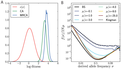
Individuals in our model have a heritable fitness which determines the distribution of the number of immediate offspring. While fit individuals have on average more offspring than less fit ones, the fitness differences in the population are small and the offspring distribution across the population is narrow. However, fitness is heritable and fit individuals can have a very large number of distant great^t-grandchildren. Hence the distribution of offspring after $t$ generations, $P(n,t)$, will be dominated by fit individuals and can have a very long tail. Conversely, the present day population has fewer and fewer ancestors as we trace its lineages backwards in time. At $T_{MRCA}$ generations in the past, there is exactly one individual that is the ancestor to the entire population. Ancestors of the MRCA are also common ancestors (CA) of the entire population, albeit not the most recent one. Fig. 5 shows that MRCAs and CAs tend to come from the high fitness tail of the population. MRCAs tend to be fitter than CAs, since they are conditioned on giving rise to at least two lineages that persist to the present.

The offspring distribution, $P(n,t)$, changes slowly from the initial narrow distribution to a broad distribution with a power-law at intermediate times Neher:2011p42539 . The broad distribution at intermediate times is at the heart of the correspondence of genealogies in models of adapting populations and the Bolthausen-Sznitman coalescent.

The BSC assumes that all individuals are exchangeable and that in every coalescent event a randomly chosen set of lineages merges into one. Each possible merger event has a specific rate associated with it, and the rate at which $k$ individuals merge into one common ancestor is $q_{k}=T_{2}^{-1}(k-1)^{-1}$ Berestycki:2009p45808 (the general expression for the rates is given below in Eq. (7)). In contrast, in the neutral coalescent, higher order coalescence is very rare $\propto N^{-(k-1)}$. We will present the basic properties of the BSC briefly in the discussion.

To appreciate how these coalescence rates can emerge from a model with selection, consider the number of individuals $n_{i}$ that descend from an individual $i$ that lived $t$ generations in the past. The probability that $k$ individuals sampled randomly from the population have a common ancestor $t$ in the past is then given by

$$Q_{k}(t)=\left\langle\sum_{i=1}^{N}\left(\frac{n_{i}}{\sum_{j}n_{j}}\right)^{k}\right\rangle\ ,$$ (3)

where the average $\langle.\rangle$ is over all $n_{i}$. $Q_{k}(t)$ is dominated by $n_{i}\gg k$ such that sampling with replacement in Eq. (3) is an accurate approximation. Using the identity $\Gamma(k)C^{-k}=\int_{0}^{z}dz\,z^{k-1}e^{-zC}$ and assuming that $t$ is small enough that the different $n_{i}$ are still approximately independent, we can express $Q_{k}$ as

$$\begin{split}Q_{k}(t)&\approx\frac{N}{\Gamma(k)}\int_{0}^{\infty}dzz^{k-1}\langle e^{-zn}\rangle^{N-1}\langle n^{k}e^{-zn}\rangle\\ &\approx-\frac{N}{\Gamma(k)}\int_{0}^{\infty}dzz^{k-1}e^{-N\Phi_{z}(t)}(-1)^{k}\partial_{z}^{k}\Phi_{z}(t)\ ,\end{split}$$ (4)

where we introduced the Laplace transform $1-\Phi_{z}(t)=\sum_{n}e^{-zn}P(n,t)$ and assumed $N\Phi_{z}^{2}(t)\ll 1$. In the SI, we show that $\Phi(t)\sim z^{\frac{\sigma^{2}}{2Dt}}$ for $t>T_{delay}=\sigma^{2}/2D$. For a limited interval after $t>T_{delay}$, we find that the probability that $k$ individuals have a common ancestor increases with rate

$$q_{k}=\frac{2D}{\sigma^{2}}\frac{1}{k-1}$$ (5)

per unit time. More general coalescence rates can be calculated analogously; see SI. Prior to $T_{delay}$, the rate of coalescence is very low. This is in agreement with Fig. 3, where we found that little coalescence happened early, while coalescence times are exponentially distributed after that with characteristic time $T_{c}\approx\sigma^{2}/2D$ for $t>T_{delay}$. The relative rates of mergers of 2,3,…are consistent with the BSC, explaining our observations for the frequency spectrum and the time to the most recent common ancestor.

The branching process approximation used to derive the result Eq. (5) is valid only for short times but nevertheless gives us the relative rates of multiple mergers once coalescence sets in. For subsequent deeper coalescent events, the relevant lineages are already at the tip of the fitness distribution, and this process repeats itself without the delay. In fact, after this delay all remaining lineages are in a narrow region at the tip of the fitness distribution. The situation now resembles that of coalescence in FKPP waves: The fitness of the lineages is roughly equal, but lineages have to stay ahead of a fitness cut-off in order to survive. We can therefore employ the phenomenological theory of genealogies in FKPP waves from Brunet:2006p47336 , which confirms the above result for the coalescent time scale; see SI. We present an additional argument based on “tuned” models introduced in Hallatschek:2011p39697 in the SI.

To corroborate our analysis, we performed additional simulations that allow us to measure the Laplace transform of the distribution of pair coalescent times for very large populations. These simulations show that the pair coalescent time is indeed exponential with characteristic time $\sigma^{2}/2D$ after a delay of the same length; see Fig. 6. The algorithm used is similar in spirit to the algorithm by Brunet et al.  Brunet:2007p18866 ; see SI.

Strictly speaking, the analogy to an exchangeable coalescent model like the Bolthausen-Sznitman coalescent requires that different coalescence events one lineage undergoes be independent. For this to be true, individuals descending from a lineage have to distribute evenly across the fitness distribution $c(x)$ between coalescence events, which requires a time $T_{eq}\approx T_{c}$. Hence we should not expect a clean convergence towards the Bolthausen-Sznitman coalescent. Nevertheless, we find it to be a very good model for the observed genealogies after accounting for the delay. The underlying reason is that local equilibration in the region where the ancestral lineages are is fast ($t\approx D^{-1/3}$). This region, however, undergoes fluctuations on the time scale $T_{eq}$, which modulate the overall rate of coalescence but do not significantly affect the local dynamics. For waves of FKPP type that describe the spread of individuals in space, $T_{eq}\ll T_{c}$ in large populations Brunet:2007p18866 .

Figure 5: Panel A shows the distribution of the log-fitness of all CAs and all MRCAs compared to the average distribution, $c(x)$, of log-fitness in the population; see text. These distributions were measured in forward simulations with $\mu=1,\,s=0.01$ and $N=10^{6}$. Panel B: Site frequency spectrum of derived neutral alleles in a background selection scenario with deleterious mutations of effect $s$. As the ratio $\mu/s$ is varied while keeping $\sigma^{2}=\mu s=0.1$ constant, the SFS interpolates between the expectation for the Kingman and the BS coalescent. $N=10^{4}$.

IV Discussion

We have shown that in a simple model of adapting populations, the observed genealogies are inconsistent with the standard neutral coalescent. Instead, genealogical trees are characterized by long terminal branches and almost simultaneous coalescence of multiple lineages. At branching events deep in the tree, one commonly observes that almost all individuals of the population descend from one branch, whereas very few descent from the other branches. Such skewed branching is unlikely in neutral coalescent models, regardless of the history of the effective population size. One consequence of these uneven branching ratios is a non-monotonic site frequency spectrum (SFS) of derived neutral alleles. Compared to the neutral coalescent, the low frequency part of the SFS is much steeper, whereas the high frequency part shows a characteristic up-turn; see Fig. 4.

A given pair of lineages is unlikely to coalesce in the bulk of the fitness distribution. Typically, both lineages move into the high fitness tip of the population distribution before they coalesce as illustrated in Fig. 2. This results in long terminal branches and a distribution of heterozygosities peaked at intermediate values. After this delay, the typical time to coalescence is again on the order of the time it takes the fittest individuals to dominate the population; see Fig. 3. In panmictic populations, this time depends on the logarithm of the population size and in our model is proportional to $(\log\tilde{N})^{1\over 3}$.

We argue that the exponential amplification of fit lineages is responsible for these observations and that coalescence in such rapidly adapting populations is generically described by a modified Bolthausen-Sznitman coalescent (BSC) Bolthausen:1998p47390 ; Berestycki:2009p45808 . The BSC is a special case of the large class of $\Lambda$-coalescent processes Pitman:1999p41045 . Given the distribution $p(f)$ of the fraction $f$ of the population that descends from a single individual in the previous generation, the rate at which $k$ out of $b$ lineages merge is given by

$$\begin{split}\lambda_{b,k}&=\int dfp(f)f^{k}(1-f)^{b-k}\ .\end{split}$$ (6)

The Bolthausen-Sznitman coalescent corresponds to $p(f)\sim f^{-2}$ for large $f$, in which case Eq. (7) reduces to

$$\lambda_{b,k}=\frac{1}{T_{c}}\frac{(k-2)!(b-k)!}{(b-1)!}$$ (7)

or Eq. (5) for the special case $b=k$. The total rate at which coalescence events happen in a sample of $k$ lineages is therefore

$$\lambda_{b}=\sum_{k}{b\choose k}\lambda_{b,k}=\frac{b-1}{T_{c}}\ ,$$ (8)

in contrast to the neutral coalescent, where $\lambda_{b}\propto b(b-1)$. A coalescence event reduces the number of surviving lineages on average by $\log b$ such that the average rate at which the number of lineages decreases is $\approx T_{c}^{-1}b\log b$. The typical time needed to reach the common ancestor of a sample of size $n$ is $\approx T_{c}\log\log n$, in contrast to $2T_{c}$ in Kingman’s coalescent. The BSC occupies a special intermediate position between Kingman’s coalescent, where only pairwise mergers are allowed, and a star-coalescent, where all lineages coalesce simultaneously. Star-like genealogies are expected in rapidly expanding populations or in a region fully linked to a recent rapid hard sweep Slatkin:1991p43283 . In the BSC, multiple mergers (subsets of lineages with star-like trees) are frequent, but at the same time there are many mergers at different depth in the tree. In fact, the BSC is the $\alpha=1$ case of the one parameter family of Beta-coalescents with parameter $0<\alpha<2$, while the case $\alpha\to 2$ corresponds to the Kingman coalescent. For a more in depth discussion, see the recent review by Berestycki Berestycki:2009p45808 . The BSC is easily implemented as a computer simulation by drawing an exponentially distributed random number with mean $\lambda_{b}^{-1}$ to determine the time of the next event. The type of event is then chosen with probabilities proportional to $\lambda_{b,k}$.

The models of adaptation we have studied have a narrow offspring distribution. Nevertheless, the exponential amplification of fit genotypes over many generations gives rise to a distribution of clone sizes with the required asymptotic behavior. The important lineages are those that run ahead of the distribution, expand faster, and take over a significant fraction of the population Brunet:2006p47336 . Over even longer times, the fitnesses of ancestors and descendants decorrelate. This allows us to approximate the genealogies with the abstract BSC, which assumes that there are no correlations in offspring number across generations.

Conventionally, an increased variance in offspring number is accounted for by defining an effective population size. With a clone size distribution $p(f)\sim f^{-2}$, however, the variance diverges with the population size Neher:2011p42539 . Similar effects arise in other models with very skewed offspring distribution Eldon:2006p36003 . As a consequence, the genealogies are dominated by rare anomalously large clones and described by the BSC rather than Kingman’s coalescent. The rate of coalescence is not set by $N^{-1}$ but by the rate at which clones expand and collapse. We would like to stress that evolutionary dynamics thereby remains highly stochastic, even in very large populations. Analogous behavior has recently been observed in models of individuals invading uninhabited territory (FKPP type waves) Brunet:2007p18866 and ensembles of super-critical branching processes Schweinsberg:2003p40932 .

The BSC is not only a good model for genealogies of adapting asexual populations but also applies to populations under purifying selection in which Muller’s ratchet clicks often. The standard model for the distortion of genealogies by purifying selection assumes that deleterious mutations are rapidly purged and coalescence is neutral in the mutation free class with a reduced population size $Ne^{-\mu/s}$, where $\mu$ is the deleterious mutation rate and $s$ is the effect size of deleterious mutations Charlesworth:1993p36005 . More elaborate analysis based on a fitness-class coalescent explicitly tracks lineages through the population and calculates the contribution to coalescence before lineages reach the mutation free class Walczak:2011p45228 . However, all of this only holds as long as the mutation free class is large and Muller’s ratchet does not operate, which requires $Nse^{-\mu/s}\gg 1$ Stephan:1993p42929 ; Jain:2008p45047 ; Neher:2012p47353 . Fig. 5B shows the SFS of derived neutral alleles for different ratios $\mu/s$. For small $\mu/s$, the SFS is similar to those of Kingman’s coalescent with a reduced time to coalescence, in accordance with the background selection theory. However, as soon as the ratchet starts to click frequently, the SFS develops the non-monotonicity characteristic of the Bolthausen-Sznitman coalescent.

If the ratchet is clicking fast, the fitness distribution in the population resembles that of traveling wave models, but selection on fitness variation can not keep up with the influx of deleterious mutations. Similarly, populations in a steady balance between deleterious and beneficial mutations Goyal:2012p47382 have genealogies as found here for rapidly adapting populations. The reason for the qualitative difference in the ratchet regime is the fact that the nose of the wave is not steady, but constantly turning over. Different lineages are struggling to get ahead of everybody else and, in the frame of reference of the population (that is, relative to mean fitness), are exponentially amplified. In contrast, dynamics of lineages in the mutation free class is neutral if Muller’s ratchet does not operate.

In the supplementary material, we show that the argument that gave rise to the particular coalescence rates in Eq. (5) can be extended to a large class of models that are controlled by a small and fluctuating population of highly fit individuals. We thus argue that the Bolthausen-Sznitman coalescent generically emerges as a consequence of the exponential amplification of the clones descending from these highly fit individuals, together with the seeding of novel lineages. The latter could happen via lucky diffusion to high fitness (our model here), via large effect beneficial mutations, or via lucky outcrossing. After some time, the distribution of lineage size follows a power law with an exponent close to -2 Yule:1925p38579 ; Desai:2007p954 ; Neher:2011p42539 . Given an effective offspring distribution of this shape, the Bolthausen-Sznitman coalescent follows Schweinsberg:2003p40932 ; Brunet:2007p18866 . In desai_genetic_2012 , the authors study a model where the mutation rate is much smaller than the typical effect sizes of mutations. They show that also in this case, the genealogies are well approximated by the BSC after a delay. Whether the BSC also describes genealogies in scenarios where fitness is increased in rather large increments (compared to the population diversity) Gerrish:1998p5933 ; Schiffels:2011p43799 remains an interesting topic for future work.

The compatibility of a sample with the neutral coalescent model is typically assessed using statistics such as Tajima’s $D$ Tajima:1989p37563 . Tajima’s $D$ compares the average number of pairwise differences to the total number of segregating sites in the sample. In the case of the BSC, the average pairwise diversity is proportional to $\langle T_{2}\rangle$, while the total number of segregating sites is proportional to $\langle T_{2}\rangle n/\log n$ (compared to $\langle T_{2}\rangle\log n$ for the Kingman coalescent). This tremendous excess of segregating sites is a consequence of the very steep SFS at small frequencies and results in $D\propto-\log(n)$.

Sexual populations and recurrent selective sweeps at linked loci can also give rise to multiple mergers in the genealogies Durrett:2005p40919 . However, recombination and sexual reproduction will reduce the effects of linked selection and decouple the genealogies of different loci. Hence we expect that the coalescent behavior crosses over to Kingman’s coalescent as the recombination rate increases – at least in models of panmictic populations. This is indeed observed in models of facultatively sexual populations Neher:2011p42539 .

Given the apparent universality of the Bolthausen-Sznitman coalescent in spatially expanding populations and panmictic adapting populations, it should be included as a prior in popular population genetic and phylogenetic inference programs such as BEAST Drummond:2007p30127 .

V Acknowledgements

We are grateful for many stimulating discussions with Boris Shraiman, Aleksandra Walczak, Michael Desai, Daniel Fisher, Trevor Bedford, and Martin Möhle. We also would like to thank Kari Küster for coding some of the simulations used in early stages of this work and Lukas Geyrhofer for help with tuned models. This research was supported by the ERC through Stg-260686 to RAN.

Appendix A Derivation and limitations of Eq. 1

We assume a population of $N$ individuals that replicate at rate $B$, die at rate $D$, and mutate at rate $\mu$. For convenience, we measure time in units of generations and set birth and death rate to $B=\exp(y-\lambda)$ and $D=1$, respectively. Here, $y$ is the log-fitness of the individual in question, while the population size is kept constant by adjusting $\lambda$. Typically, $\lambda$ is equal to the sum of the mean log-fitness and a small modulation that increases growth rate when the population size falls below the target $N_{0}$ and decreases growth rate otherwise. We use $\lambda=\bar{y}-(1-NN_{0}^{-1})$ which keeps $N$ within $\mathcal{O}(\sqrt{N_{0}})$ of $N_{0}$. For present purposes, this model is equivalent to a model with strictly constant population size. Different forms of $\lambda$ that constrain the population size to a different degree are possible Hallatschek:2011p39697 . Mutations increment the log-fitness $y$ of an individual by $\delta$ drawn from a distribution $K(\delta)$. Disregarding fluctuations and assuming fitness differences are small, the distribution of fitness in the population, $c(y,t)$, obeys the following deterministic equation

$$\partial_{t}c(y,t)=(y-\lambda)c(y)+\mu\int ds\,K(\delta)\left[c(y-\delta,t)-c(y,t)\right]$$ (9)

Generically, steady state solutions to this equation oscillate around $0$ for large $y-\bar{y}$, where the stochastic effects of finite populations become important Cohen:2005p45154 . The magnitude of stochastic perturbations to the population in the interval $\left[y,y+\Delta y\right]$ are proportional to $\sqrt{c(y)\Delta y}$ and can be accounted for either by an explicit model of discrete particles, or a stochastic partial-differential equation

$$\partial_{t}c(y,t)=(y-\lambda)c(y)+\mu\int d\delta\,K(\delta)\left[c(y-\delta,t)-c(y,t)\right]+\sqrt{c(y,t)}\eta(y,t)$$ (10)

where $\eta(y,t)$ is Gaussian white noise with $\langle\eta(y,t)\eta(y+x,t^{\prime})\rangle=\delta(x)\delta(t-t^{\prime})$ Hallatschek:2011p39697 . This stochasticity determines the average steady state velocity, which diverges in the limit $N\to\infty$ Rouzine:2003p33590 ; Desai:2007p954 ; Cohen:2005p45154 .

If the mutation rate $\mu$ is large and the distribution $K(\delta)$ falls off quickly enough such that the typical mutations are small, one can expand $c(y-\delta,t)$ inside the integral to obtain

$$\partial_{t}c(y,t)\approx(y-\lambda)c(y,t)+\frac{\mu\langle\delta^{2}\rangle}{2}\frac{\partial^{2}}{\partial y^{2}}c(y,t)-\mu\langle\delta\rangle\frac{\partial}{\partial y}c(y,t)+\sqrt{c(y,t)}\eta(y,t)$$ (11)

where $\langle\ldots\rangle$ denotes the average over $K(\delta)$. The expansion of $c(y-\delta,t)$ is a good approximation as long as the mutation rate is larger than typical mutational effects. Specifically, it is required that $\mu^{2}/\langle\delta^{2}\rangle>(\log\tilde{N})^{2}$, see Cohen:2005p45154 for a discussion of this issue. This condition will limit the applicability of the model to RNA virus populations or asexual eukaryotes with long genomes. We find, however, that the basic features of the BSC are also present in models where $\mu/\sqrt{\langle\delta^{2}\rangle}\ll 1$, see supplementary figures 9 and 10 below. This observation is confirmed by a recent preprint by Desai et al desai_genetic_2012 , in which the authors investigate a model with $\mu^{2}\ll\langle\delta^{2}\rangle$.

The average of the population distribution governed by Eq. (11) obtains a steady shape that translates towards higher $y$ with a velocity $v=\sigma^{2}+\mu\langle\delta\rangle$, where

$$\sigma^{2}\approx D^{2\over 3}\left(24\log(ND^{1\over 3})\right)^{1\over 3}$$ (12)

and $D=\frac{\mu\langle\delta^{2}\rangle}{2}$. In a suitably chosen comoving frame $x=y-vt$, the equation describing the population distribution simplifies to

$$0\approx xc(x,t)+D\frac{\partial^{2}}{\partial x^{2}}c(y,t)+\sigma^{2}\frac{\partial}{\partial x}c(x,t)+\sqrt{c(x,t)}\eta(x,t)$$ (13)

If the mutational input $\mu\langle\delta\rangle=0$, the average velocity equals the fitness variance $\sigma^{2}$ of the population. If deleterious mutations are more common than beneficial mutations and on average reduce fitness, the velocity will be smaller than the fitness variance by $|\mu\langle\delta\rangle|$. Eq. (13) has been studied in detail in Cohen:2005p45154 . In large population, the typical solution in the quasi-steady state is given by

$$c(x)=\begin{cases}Ce^{-\frac{\sigma^{2}x}{2D}}\mathrm{Ai}\left(\frac{\sigma^{4}}{4D^{4\over 3}}-\frac{x}{D^{1\over 3}}\right)&x<x_{c}\\ De^{-\frac{\sigma^{2}x}{D}}&x>x_{c}\end{cases}$$ (14)

where $x_{c}$ and $D$ are determined by matching $c(x)$ and $\partial_{x}c(x)$ at $x_{c}$, while $C$ is set by the normalization.

Appendix B Frequency spectrum of derived alleles in the BSC

A mutation occurring on some branch of the genealogy will be present in all individuals that descend from the branch considered. Very recent mutations tend to be rare, while old mutations can be common. The number of leafs descending from lineages at a time $\tau=T/T_{c}$ in the past is also known as the size of the $\tau$-families ($T_{c}$ is the coalescent time scale). These family sizes follow a two parameter Poisson-Dirichlet distribution $PD(0,e^{-\tau})$ and the size $z$ of the first block is Beta distributed as Berestycki:2009p45808

$$P(z,\tau)=\frac{z^{-e^{-\tau}}(1-z)^{e^{-\tau}-1}}{\Gamma(1-e^{-\tau})\Gamma(e^{-\tau})}$$ (15)

Common mutations, i.e., those present in the majority of the population, most likely fall onto this block. The present day frequency of the derived allele is equal to the block size. If neutral mutations occur at rate $\mu$, we can calculate the ensemble averaged site frequency spectrum (SFS) by integrating over all times at which the mutation could have occurred. Ignoring mutations that fall onto other blocks of the Poisson-Dirichlet distribution, the average SFS is given by

$$\begin{split}f(\nu)&=\mu\int_{0}^{\infty}dT\frac{\nu^{-e^{-\tau}}(1-\nu)^{e^{-\tau}-1}}{\Gamma(1-e^{-\tau})\Gamma(e^{-\tau})}\\ &=\mu T_{c}\int_{0}^{\infty}d\tau\frac{\nu^{-e^{-\tau}}(1-\nu)^{e^{-\tau}-1}}{\Gamma(1-e^{-\tau})\Gamma(e^{-\tau})}\\ &=\mu T_{c}\int_{0}^{1}dy\frac{\nu^{-y}(1-\nu)^{y-1}}{y\Gamma(1-y)\Gamma(y)}\\ &=\mu T_{c}\int_{0}^{1}dy\frac{\sin(\pi y)\nu^{-y}(1-\nu)^{y-1}}{\pi y}\end{split}$$ (16)

where we have used Euler’s reflection formula for the Gamma functions. The last integral has an expression in terms of special functions. However, the term $\sin(\pi y)/\pi y$ is close to one for small $y$ where the dominant contribution to the integral comes from. Hence we have approximately

$$f(\nu)\approx\mu T_{c}\int_{0}^{1}dy\nu^{-y}(1-\nu)^{y-1}=\mu T_{c}\frac{2\nu-1}{\nu(1-\nu)(\log\nu-\log(1-\nu))}$$ (17)

Higher order corrections to Eq. (17) can be obtained by expanding the sine to higher order. They do not change the result qualitatively. For common derived alleles with $1-\nu\ll 1$, the above restriction to the first block of the Poisson-Dirichlet distribution is a good approximation since other blocks are almost always short $z\ll 1$. In the limit $1-\nu\ll 1$, the expression simplifies to

$$f(\nu)\approx-\frac{\mu T_{c}}{(1-\nu)\log(1-\nu)}$$ (18)

which coincides with Eq. (2) of the main text. For $1-\nu\ll 1$, it describes the simulation data very well, see Fig. 4. At the rare end of the spectrum, the observed power law $f(\nu)\sim\nu^{-2}$ is a (well-known) consequence of exponentially growing sub-populations Yule:1925p38579 , corresponding to expanding clones in the high-fitness tip of the traveling wave.

Appendix C Generating function of the offspring number distribution

To calculate the moments of the lineage size distribution, we need the distribution $P(n,t|x,t_{0})$ of lineage sizes $n$ at time $t$, given the lineage was seeded a fitness $x$ above the mean at time $t_{0}$. $P(n,t|x,t_{0})$ obeys the backward equation

$$\begin{split}P(n,t|x+v\Delta t,t_{0}-\Delta t)=&\left[1-\Delta t(2+x+\mu)\right]P(n,t|x,t_{0})+\Delta t(1+x)\sum_{n^{\prime}}P(n^{\prime},t|x,t_{0})P(n-n^{\prime},t|x,t_{0})\\ &+\Delta t\delta_{n,0}+\Delta t\mu\int ds\,K(\delta)P(n,t|x+\delta,t_{0})\end{split}$$ (19)

where $K(\delta)$ is a normalized distribution of mutational effects as used in Sec. A and we have used $1+x$ as birth rate and $1$ as death rate. The first term gives the probability that no birth, death, or mutation is happening in the interval $\Delta t$, the second term corresponds to birth, the third term to loss of the lineage ($n=0$) and the last term to a mutation changing the log-fitness by $\delta$. Rearranging and taking the limit $\Delta t\to 0$ yields

$$\begin{split}-\partial_{t_{0}}P(n,t|x,t_{0})+v\partial_{x}P(n,t|x,t_{0})=&-(2+x+\mu)P(n,t|x,t_{0})+(1+x)\sum_{n^{\prime}}P(n^{\prime},t|x,t_{0})P(n-n^{\prime},t|x,,t_{0})\\ &+\delta_{n,0}+\mu\int d\delta\,K(s)P(n,t|x+\delta,t_{0})\end{split}$$ (20)

Using the time translation invariance, $P(n,t|x,t_{0})=P(n,t-t_{0}|x,0)$, and defining $\psi_{z}(x,t)=\sum_{n}e^{-zn}P(n,t|x,0)$, we find

$$\partial_{t}\psi_{z}(x,t)+v\partial_{x}\psi_{z}(x,t)=1-(2+x)\psi_{z}(x,t)+(1+x)\psi_{z}^{2}(x,t)+\mu\int ds\,K(\delta)[\psi_{z}(x+\delta,t)-\psi_{z}(x,t)]$$ (21)

Upon multiplying by $-1$ and substituting $\phi_{z}(x,t)=1-\psi_{z}(x,t)$, this equation simplifies to

$$\partial_{t}\phi_{z}(x,t)+v\partial_{x}\phi_{z}(x,t)=x\phi_{z}(x,t)-\phi_{z}^{2}(x,t)+\mu\int ds\,K(\delta)[\phi_{z}(x+\delta,t)-\phi_{z}(x,t)]$$ (22)

where we have approximated $(1+x)\phi_{z}^{2}$ by $\phi_{z}^{2}$, which amounts to assuming that all relevant $x\ll 1$ and selection is important only over many generations. Note the similarity of this equation to Eq. (9) governing the fitness distribution of the population. In analogy to Sec. A we can expand $\phi_{z}(x+\delta,t)$ inside the integral if the mutation rate is large and $K(\delta)$ falls of rapidly with $|\delta|$ and obtain

$$\partial_{t}\phi_{z}(x,t)=x\phi_{z}(x,t)-\sigma^{2}\partial_{x}\phi_{z}(x,t)+\frac{\mu\langle\delta^{2}\rangle}{2}\partial_{x}^{2}\phi_{z}(x,t)-\phi_{z}^{2}(x,t)$$ (23)

where $\sigma^{2}=v-\mu\langle\delta\rangle$ accounts for both the actual translation of the population along the fitness axis and the mutation load. Defining $D=\frac{\mu\langle\delta^{2}\rangle}{2}$, we have the following equation for the generating function

$$\partial_{t}\phi_{z}(x,t)=x\phi_{z}(x,t)-\sigma^{2}\partial_{x}\phi_{z}(x,t)+D\partial_{x}^{2}\phi_{z}(x,t)-\phi^{2}_{z}(x,t)$$ (24)

with initial condition $\phi_{z}(x,0)=1-e^{-z}$. This equation allows two approximate solutions for small and large $x$. For small $x$, $\phi_{z}(x,t)$ is small we can neglect the non-linearity. Conversely, at large $x$, we find that $\phi_{z}(x,t)$ is large and the dominant balance is between the terms $x\phi_{z}(x,t)$ and $\phi_{z}^{2}(x,t)$ while the first and second derivative can be neglected. Using these approximations and assuming $z\ll 1$, we can solve Eq. (24) for small $x$ and large $x$ and match the two asymptotic solutions.

$$\phi_{z}(x,t)\approx\begin{cases}ze^{xt+\frac{Dt^{3}}{3}-\frac{\sigma^{2}t^{2}}{2}}&x<x^{*}\\ x&x>x^{*}\end{cases}$$ (25)

The crossover is approximately at $x^{*}=\frac{\sigma^{2}t}{2}-\frac{Dt^{2}}{3}-\frac{\log z/x^{*}}{t}$. Note that the branching process description is only valid for a time before population size constraints have to be imposed and lineages cease to be approximately independent Cohen:2005p45154 ; Hallatschek:2011p39697 . At short times, however, it is a valid approximate description of the number of offspring of a marked individual. We are interested foremost in the distribution of offspring averaged over the population $c(x)$, see Eq. (13). For short times with $x_{c}<x^{*}$ we have

$$\Phi(z,t)=zAe^{-\frac{\sigma^{2}t^{2}}{2}+\frac{Dt^{3}}{3}}\int^{x_{c}}dx\mathrm{Ai}\left(\frac{\sigma^{4}}{4D^{4\over 3}}-\frac{x}{D^{1\over 3}}\right)e^{x\left(t-\frac{\sigma^{2}}{2D}\right)}$$ (26)

We see that the behavior of this average changes qualitatively as $t>\frac{\sigma^{2}}{2D}$ when it starts to be boundary dominated. Assuming $x^{*}<x_{c}$, i.e., the saturation of $\phi_{z}(x,t)$ happens within the validity of the Airy function solution, we have

$$\Phi(z,t)\approx zAe^{-\frac{\sigma^{2}t^{2}}{2}+\frac{Dt^{3}}{3}}\int^{x^{*}}dx\mathrm{Ai}\left(\frac{\sigma^{4}}{4D^{4\over 3}}-\frac{x}{D^{1\over 3}}\right)e^{x\left(t-\frac{\sigma^{2}}{2D}\right)}+x^{*}A\int_{x^{*}}^{x_{c}}dx\mathrm{Ai}\left(\frac{\sigma^{4}}{4D^{4\over 3}}-\frac{x}{D^{1\over 3}}\right)e^{-\frac{x\sigma^{2}}{2D}}$$ (27)

Both of these integrals are dominated by a narrow region in the vicinity of $x^{*}$. Plugging in the definition of $x^{*}$, we find

$$\begin{split}\Phi(z,t)&\approx x^{*}Ae^{-\frac{x^{*}\sigma^{2}}{2D}}\left[\int^{0}d\delta x\mathrm{Ai}\left(\frac{\sigma^{4}}{4D^{4\over 3}}-\frac{x^{*}+\delta x}{D^{1\over 3}}\right)e^{\delta x(t-\frac{\sigma^{2}}{2D})}+\int_{0}d\delta x\mathrm{Ai}\left(\frac{\sigma^{4}}{4D^{4\over 3}}-\frac{x^{*}+\delta x}{D^{1\over 3}}\right)e^{-\frac{\delta x\sigma^{2}}{2D}}\right]\\ &=C(t,x^{*})e^{-\frac{x^{*}\sigma^{2}}{2D}}=C(t,x^{*})e^{\frac{\sigma^{2}\log z/x^{*}}{2Dt}+\frac{\sigma^{4}t}{4D}-\frac{\sigma^{2}t^{2}}{6}}=E(t,x^{*})z^{\frac{\sigma^{2}}{2Dt}}\end{split}$$ (28)

where $C(t,x^{*})$ and $E(t,x^{*})$ depend only weakly on $x^{*}$. The $k$th derivative of $\Phi(z,t)$ with respect to $z$ is therefore

$$\partial_{z}^{k}\Phi(z,t)\approx z^{-k}\Phi(z,t)\prod_{i=1}^{k-1}(\frac{\sigma^{2}}{2Dt}-i)=(-1)^{k}z^{-k}\Phi(z,t)\prod_{i=0}^{k-1}(i-\frac{\sigma^{2}}{2Dt})$$ (29)

We can now evaluate the probability $Q_{k}$ that a set of $k$ lineages merges into one:

$$\begin{split}Q_{k}(t)&\approx-\frac{N}{\Gamma(k)}\int_{0}^{\infty}dzz^{k-1}e^{-N\Phi(z,t)}(-1)^{k}\partial_{z}^{k}\Phi(z,t)\\ &\approx-\frac{\prod_{i=0}^{k-1}(i-\frac{\sigma^{2}}{2Dt})}{\Gamma(k)}\int_{0}^{\infty}dzz^{-1}e^{-N\Phi(z)}N\Phi(z,t)\\ &\approx-\frac{2Dt}{\sigma^{2}}\frac{\prod_{i=0}^{k-1}(i-\frac{\sigma^{2}}{2Dt})}{\Gamma(k)}\int_{0}^{\infty}d\phi\,e^{-\phi}=\frac{\prod_{i=1}^{k-1}(i-\frac{\sigma^{2}}{2Dt})}{\Gamma(k)}\ .\end{split}$$ (30)

Defining $\tau$ as $\tau=\frac{2Dt}{\sigma^{2}}$, we have

$$Q_{k}(t)=\frac{\Gamma(k-\tau^{-1})}{\Gamma(1-\tau^{-1})\Gamma(k)}\ .$$ (31)

For large $\tau$, all $Q_{k}$ become equal, which simply means that the population has coalesced into its common ancestor. For $t=\frac{\sigma^{2}}{2D}+\delta t$, we can differentiate with respect to $\delta t$ and obtain

$$q_{k}=\partial_{t}Q_{k}(t)|_{t=\sigma^{2}/2D}=\frac{2D}{\sigma^{2}}\frac{1}{k-1}\ ,$$ (32)

which are the Bolthausen-Sznitman merger rates.

Similarly, we can calculate more general merger probabilities such as the probability that $k$ out of $b$ lineages have merged, while all other $b-k$ lineages trace back to distinct ancestors. Making again the assumption of independent lineages and accounting for the possibilities of choosing $b-k+1$ ordered lineages as ancestors, we have

$$\begin{split}\Lambda_{b,k}&=\frac{\Gamma(N+1)}{\Gamma(N-b+k)}\left\langle\left(\sum_{j}n_{j}\right)^{-b}n_{1}^{k}\prod_{i=1}^{b-k}n_{i+1}\right\rangle\\ &\approx\frac{\Gamma(N+1)}{\Gamma(N-b+k)\Gamma(b)}\int_{0}^{\infty}dz\,z^{b-1}\langle n^{k}e^{-zn}\rangle\langle ne^{-zn}\rangle^{b-k}\langle e^{-zn}\rangle^{N-b+k-1}\\ &=\frac{\Gamma(N+1)}{\Gamma(N-b+k)\Gamma(b)}\int_{0}^{\infty}dz\,z^{b-1}(-1)^{k+1}[\partial_{z}^{k}\Phi(z,t)][\partial_{z}\Phi(z,t)]^{b-k}e^{-(N-b+k-1)\Phi}\end{split}$$ (33)

Using $\partial_{t}\Phi(z,t)=\frac{\sigma^{2}}{2Dt}z^{-1}\Phi(z,t)$, defining $\gamma=\frac{\sigma^{2}}{2Dt}$, and assuming $N\gg b$, we have

$$\begin{split}\Lambda_{b,k}&=\frac{\gamma^{b-k}\Gamma(N+1)}{\Gamma(N-b+k)\Gamma(b)}\int_{0}^{\infty}dz\,z^{k-1}(-1)^{k+1}[\partial_{z}^{k}\Phi(z,t)]\Phi(z,t)^{b-k}e^{-(N-b+k-1)\Phi}\\ &\approx-\prod_{i=0}^{k-1}(i-\gamma)\frac{\gamma^{b-k}}{\Gamma(b)}\int_{0}^{\infty}dz\,z^{-1}[N\Phi(z,t)]^{b-k+1}e^{-N\Phi}\end{split}$$ (34)

Changing integration variables to $\phi=N\Phi(z,t)$, we find

$$\begin{split}\Lambda_{b,k}&\approx-\prod_{i=0}^{k-1}(i-\gamma)\frac{\gamma^{b-k-1}}{\Gamma(b)}\int_{0}^{\infty}d\phi\,\phi^{b-k}e^{-\phi}\\ &\approx-\prod_{i=0}^{k-1}(i-\gamma)\frac{\gamma^{b-k-1}\Gamma(b-k+1)}{\Gamma(b)}=\gamma^{b-k}\frac{\Gamma(k-\gamma)(b-k)!}{\Gamma(1-\gamma)(b-1)!}\end{split}$$ (35)

For $t=\frac{\sigma^{2}}{2D}+\delta t$ with $\delta t\ll\frac{\sigma^{2}}{2D}$, $\gamma\approx 1$ and we find

$$\begin{split}\Lambda_{b,k}&\approx\delta t\frac{2D}{\sigma^{2}}\frac{(k-2)!(b-k)!}{(b-1)!}=\delta t\lambda_{b,k}\end{split}$$ (36)

which are the general BSC rates $\lambda_{b,k}$.

We have assumed a steady distribution with a well-defined cutoff at $x_{c}$. The actual high fitness end of the population fluctuates quite a bit, which would result in large population size fluctuations if the population size was not tightly controlled via a mean fitness that is catching up. This feed back via the mean fitness, however, is delayed and does not affect the dynamics at the nose instantaneously. The mapping to the FKPP models discussed below is better suited to describe the effects of fluctuations of the nose on coalescence.

Appendix D Relation to FKPP models

After the equilibration time $T_{eq}$ the ancestors of all extant individuals are located in a region of width $\propto D^{1/3}$ in the nose of the fitness distribution roughly $x_{c}\approx\frac{\sigma^{4}}{4D}$ ahead of the mean. Within this region, the growth rate does not vary much and the deterministic population distribution is a solution of

$$D\frac{\partial c(x)}{\partial x^{2}}-\sigma^{2}\frac{\partial c(x)}{\partial x}+x_{c}c(x)=0$$ (37)

which has an exponential solution $c(x)\sim e^{-x\gamma}$ with $\sigma^{2}(\gamma)=\frac{x_{c}}{\gamma}+D\gamma$. Waves of this form select the minimal velocity corrected by a cut-off Brunet:1997p18870, which corresponds to $\sigma^{2}=2\sqrt{x_{c}D}$ and $\gamma_{0}=\sigma^{2}/2D$, consistent with Cohen:2005p45154 . Brunet et al. Brunet:2006p47336 ; Brunet:2007p18866 have argued that the coalescence process of such waves is of Bolthausen-Sznitman type with a typical time scale given by

$$T_{c}=\frac{\log^{3}n}{\pi^{2}\gamma_{0}^{3}\alpha}=\frac{\log^{3}n}{2\pi^{2}x_{c}}$$ (38)

where $\alpha=2x_{c}\gamma_{0}^{-3}$ is the second derivative of $\sigma^{2}(\gamma)$ with respect to $\gamma$ at $\gamma=\gamma_{0}$ and $n$ is the size of the population relevant for the FKPP wave. In our case, only the part of the wave that has a substantial chance of being the common ancestor of the population is relevant and this part is located in an area of with $\mathcal{O}(D^{1/3})$ away from the tip. The number of individuals in this range is

$$\log n\propto\log\int_{-D^{1/3}}^{0}dx\,e^{-\frac{x\sigma^{2}}{2D}}\propto\frac{\sigma^{2}}{D^{2/3}}$$ (39)

Substituting this into Eq. (38) and using $x_{c}=\sigma^{4}/4D$, we find

$$T_{c}\propto\frac{\sigma^{2}}{D}$$ (40)

in agreement with the above findings. Furthermore, this argument supports our finding of Bolthausen-Sznitman coalescence after the branching process description is no longer valid.

Appendix E The BSC in tuned models

The calculation giving rise to Eq. 5 of the main text was done for a specific model of selection and mutation. We now want to argue that similar considerations hold for a large class of related models. The evolution and composition of traveling evolutionary waves is governed by the fitness distribution in the population, $c(x)$, and the probability that an individual at fitness $x$ will take over the entire population $u(x)$ Hallatschek:2011p39697 . The deterministic and linear parts (i.e., up a cutoff) of $u(x)$ and $c(x)$ are left and right eigenfunctions of the same evolution operator $\mathcal{L}$. The distribution $c(x)$ is a localized pulse, while $u(x)$ is an increasing function of $x$ (high fitness individuals have a higher chance of spreading than low fitness individuals).

Looking forward in time, $u(x)$ is the probability that a lineage at $x$ is the common ancestor of the entire population in the distant future. Before the descendants of a single lineage take over the population, they spread evenly across the fitness distribution. Once spread out, every individual is equally likely to be the common ancestor and the chance that one descendant of this lineage fixes is given by the fraction $f(x)$ of the total population made up by descendants of the lineage. Hence $u(x)$ is roughly the product of the probability that the lineage survives up to the time when it’s descendants are equally distributed across the population (establishment), and the expected fraction $f(x)$ conditional on establishment. Since only large values of $x\gg\sigma$ are relevant and the establishment probability in tuned models is $p_{est}(x)\sim x/2$, we expect $f(x)\approx 2u(x)/x$.

To analyze the coalescent properties, we need to know the distribution $p(f)$ of population fractions that trace back to single individuals a time $T_{eq}$ in the past, where $T_{eq}$ is the equilibration time of individuals across the population ($T_{eq}\approx\sigma^{2}/2D$ in our case).

$$p(f)=c(x)p_{est}(x)\left(\frac{df}{dx}\right)^{-1}$$ (41)

If the evolution operator $\mathcal{L}$ is dominated by selection all individuals that give rise to large $f$ come from the high-fitness tail. In this region, $f(x)$ rises from very low values to $\mathcal{O}(1)$, while the product of $f(x)c(x)$ (or equivalently $u(x)c(x)$) is roughly constant (viewed as a function of $f$) Hallatschek:2011p39697 . Furthermore, $f(x)$ grows exponentially with a power of $x$, implying that $f^{\prime}(x)=g(x)f(x)$ where $\log g(x)$ is a slowly varying function of $x$. Using $f^{\prime}(x)\sim f(x)$ and $c(x)\sim f(x)^{-1}$, we find

$$p(f)\sim f^{-2}$$ (42)

Given this effective off-spring distribution, we can calculate the coalescence probabilities

$$\lambda_{b,k}\sim\int df\,p(f)f^{k}(1-f)^{b-k}=\frac{(k-2!)(b-k)!}{(b-1)!}$$ (43)

which are proportional to the BSC rates. The constant of proportionality depends on the details of the stochastic dynamics which we have calculated above by other means (see also Hallatschek:2011p39697 for an alternative calculation of $Q_{2}(T_{eq})=\int dxc(x)u^{2}(x)$).

Distribution of ancestors

If $u(x)$ is the probability that a lineage with log-fitness $x$ survives to the present, the log-fitness values of common ancestors of the population are distributed as $c(x)u(x)$. Now consider the MRCA common ancestor which lived a long time in the past. By definition, the MRCA gives rise to at least two branches that survive to the present. We therefore expect that the log-fitness of an MRCA that gives rise to $k$ surviving branches should be approximately distributed as $c(x)u^{k}(x)$.

We measured the distribution of log-fitness of all common ancestors, $\mathrm{CA}$, of the population and determined $u(x)=\mathrm{CA}(x)/c(x)$, see Fig. 5A of the main text. We then compared the distribution of the log-fitness of the MRCAs of the population to $c(x)u^{2}(x)$, finding good agreement with simulations. The data is too noisy to distinguish different $c(x)u^{k}(x)$ for different $k>2$.

Appendix F Laplace transform of pair coalescence times

Instead of simulating individuals, one can also track the population density spread out on a 2 dimensional grid. To characterize diversity in an adapting population, we designate one dimension as the log-fitness axis, while the dynamics along the other direction is neutral direction. This keeps a record of the pair-coalescence time distribution as follows.

The distribution of pairwise distance between individuals along the neutral axis can be decomposed into the distribution of pairwise coalescence times and the distribution of distances along the neutral axis, given the coalescence time $T_{2}$. If individuals hop left or right with probability $\mu/2$ each, the distance distribution along the neutral direction follows a diffusion equation with diffusion constant $D=\mu/2$. Hence the averaged distribution over all pairwise differences along the neutral coordinate should be

$$P(\Delta x)=\int_{0}^{\infty}dTP(T)\frac{e^{-\frac{\Delta x^{2}}{2DT}}}{\sqrt{2\pi DT}}$$ (44)

Fourier transforming this distribution in $\Delta x$ results in

$$\hat{P}(k)=\int_{0}^{\infty}dTP(T)e^{-\frac{k^{2}DT}{2}}$$ (45)

Hence the Fourier transform of the pair-wise distance function is the Laplace transform of the pair-coalescence time in the variable $k^{2}D/2$.

We know from the individual based simulations that the coalescence process is essentially broken into two phases, a waiting period during which nothing is happening, followed by an exponential decay with charactistic time $T_{c}$. The Laplace transform of such a function is

$$\hat{P}(z)=\frac{e^{-T_{delay}z}}{1+T_{c}z}$$ (46)

These two parameters can be easily extracted by fitting this function to simulation results. Note that this Laplace transform with $z=\mu$ equals the probability of identity by state of two randomly chosen individuals.

Appendix G Simulations

G.1 Forward simulations of adapting populations

In our stochastic simulations, each individual of the population is characterized by a log-fitness that determines the expected number of offspring of this individual in the following generation. The number of offspring is Poisson distributed with a mean $\exp(y-\lambda)$, where $\lambda=\bar{y}-(1-N/N_{0})$ is a density regulating factor that keeps the population size approximately at $N_{0}$. This type of density regulation is indistinguishable from a Fisher-Wright model with exactly constant population size if $N_{0}$ is large, in which case the actual population size deviates from $N_{0}$ only by fluctuations of order $\sqrt{N_{0}}\ll N_{0}$. Individual fitness $y$ is updated via mutations drawn from a specified distribution $K(\delta)$ (in most cases a Gaussian, but we use other distributions too). The population is propagated asexually.

As the population evolves, we keep track of each individual’s parent and construct a genealogy that links each individual in the present generation to all its ancestors. All nodes of the genealogy that don’t have any offspring in the present population are deleted. From the genealogy, properties like the pair coalescent times can be easily calculated by tracing the lineages of randomly chosen individuals until they meet. Similarly, the most recent common ancestor of a population sample or the entire population can be determined this way.

Nodes in the genealogy also store how many individuals descent from them. This is convenient when calculating the site frequency spectra since a mutation that happens in a particular node of the genealogy is going to be present in all its descendants (ignoring back mutations). Since neutral mutations don’t affect the population dynamics or the genealogies, we can calculate the neutral SFS simply by summing over all opportunities for neutral mutations in the genealogy.

G.2 Bolthausen-Sznitman coalescent simulations

The direct Bolthausen-Sznitman coalescent simulations follow a backward process starting with a population of $N$ individuals. The time of the next merger event is drawn from an exponential distribution with rate given by Eq. 8 in the main text. Then the type of event and the $k$ individuals that merge are chosen according to Eq. 7 of the main text. This process is repeated until all lineages have coalesced.

G.3 Measuring the Laplace transform of $P(T_{2})$ in large populations

To measure the Laplace transform of the pair coalescence time distribution, we represent the population as a cloud on a two dimensional grid. This cloud spreads by diffusion in all directions, but is selected along one direction of grid. Diffusion is approximated as a discrete hopping process with different hopping rates in the selected and unselected directions. As explained above (Eq. (44)), the distribution of the cloud in the direction orthogonal to the direction of selection is a measure of the pair coalescence time. This distribution is measured and saved for further analysis.

G.4 Code

The source code of programs and scripts is available from the author’s website:

http://www.eb.tuebingen.mpg.de/research/research-groups/richard-neher/theoretical-population-genetics.html

Figure 6: The delay $T_{delay}$ and the coalescence time scale $T_{c}$ can be extracted from the Laplace transform of $P(T_{2})$ for very large populations and confirms that $T_{c}\approx\frac{\sigma^{2}}{2D}$.

Figure 7: The average time to the most recent common ancestor of the whole population increases relative to the time scale of coalescence with the population size $\tilde{N}=ND^{1\over 3}$. This is a well known feature of the Bolthausen-Sznitman coalescent where one expects $\langle T_{MRCA}\rangle=T_{c}\log\log N$. Panel B compares $\langle T_{MRCA}\rangle/T_{c}$ to $1+\log\log\tilde{N}$, where the additional $1$ is necessary to account for $T_{delay}\approx T_{c}$ before coalescence sets in.

Figure 8: The site frequency spectrum of neutral derived mutations in Kingman’s coalescent with constant ($\alpha=0$) and exponentially growing population sizes ($\alpha>0$ is the growth rate measured in units of $N^{-1}$). The genealogies are produced with the program ms Hudson:2002p37266 . The black lines show the theoretical expectation for a population of constant size and a rapidly expanding population. The $x$-axis is scaled as in Fig. 4 of the main text.

Figure 9: Results for an alternative models of adaptation, in which all mutations confer the same selective advantage $s$ and the mutation rate satisfies $\mu\ll s$. Panel A shows the distribution of pair coalescent times, panel B shows the site frequency spectra and the comparison to the Bolthausen-Sznitman coalescent. The times are rescaled with the prediction for the coalescent time $\langle T_{2}\rangle\approx s^{-1}\log(s\mu^{-1})$ by Desai et al. desai_genetic_2012 . Solid lines correspond to $\mu/s=0.01$, dotted lines to $\mu/s=0.1$, while $s=0.01$.

Figure 10: Results for an alternative model of adaptation, in which the selective advantage of new mutations is drawn from an exponential distribution with mean $s$, while the mutation rate satisfies $\mu\ll s$. Panel A shows the distribution of pair coalescent times, panel B shows the site frequency spectra and the comparison to the Bolthausen-Sznitman. In the absence of a prediction for the dependence of $T_{2}$ on $Ns$ or $\mu s^{-1}$, we rescale times by $s=0.01$. The mutation rate equals $\mu=0.1s$.

Figure 11: The distribution of the time to the most recent common ancestor of three individuals (panel A), and four individuals (panel B) in a model where mutational effects are normally distributed and mutations are frequent; compare Fig. 3 of the main text. Different line styles correspond to $s=0.01$ (solid), $s=0.001$ (dashed), and $s=0.0001$ (dotted), while the mutation rate is $\mu=1$. For each parameter combination, random pairs are sampled at 10000 time points $2s^{-2/3}$ generations apart

References

- (1) Kingman, J. (1982) On the genealogy of large populations. Journal of Applied Probability 19A, 27–43.
- (2) Derrida, B & Peliti, L. (1991) Evolution in a flat fitness landscape. Bulletin of Mathematical Biology 53, 355–382.
- (3) Nordborg, M. (1997) Structured coalescent processes on different time scales. Genetics 146, 1501–14.
- (4) Charlesworth, B, Morgan, M. T, & Charlesworth, D. (1993) The effect of deleterious mutations on neutral molecular variation. Genetics 134, 1289–303.
- (5) Walczak, A. M, Nicolaisen, L. E, Plotkin, J. B, & Desai, M. M. (2012) The structure of genealogies in the presence of purifying selection: A “fitness-class coalescent”. Genetics 190, 753–779.
- (6) O’fallon, B. D, Seger, J, & Adler, F. R. (2010) A continuous-state coalescent and the impact of weak selection on the structure of gene genealogies. Molecular Biology and Evolution 27, 1162–1172.
- (7) Barton, N. H & Etheridge, A. M. (2004) The effect of selection on genealogies. Genetics 166, 1115–31.
- (8) Barton, N. (1998) The effect of hitch-hiking on neutral genealogies. Genet Res 72, 123–133.
- (9) Durrett, R & Schweinsberg, J. (2005) A coalescent model for the effect of advantageous mutations on the genealogy of a population. Stochastic Process. Appl. 115, 1628–1657.
- (10) Krone, S & Neuhauser, C. (1997) Ancestral processes with selection. Theoretical population biology 51, 210–37.
- (11) Bedford, T, Cobey, S, & Pascual, M. (2011) Strength and tempo of selection revealed in viral gene genealogies. BMC Evol Biol 11, 220.
- (12) Seger, J, Smith, W, Perry, J, Hunn, J, Kaliszewska, Z, Sala, L, Pozzi, L, Rowntree, V, & Adler, F. (2010) Gene genealogies strongly distorted by weakly interfering mutations in constant environments. Genetics 184, 529.
- (13) Strelkowa, N & Lassig, M. (2012) Clonal interference in the evolution of influenza. Genetics.
- (14) Pitman, J. (1999) Coalescents with multiple collisions. Ann. Probab. 27, 1870–1902.
- (15) Berestycki, N. (2009) Recent progress in coalescent theory. arXiv math.PR/0909.3985.
- (16) Bolthausen, E & Sznitman, A.-S. (1998) On Ruelle’s probability cascades and an abstract cavity method. COMMUNICATIONS IN MATHEMATICAL PHYSICS 197, 247–276.
- (17) Brunet, E, Derrida, B, Mueller, A. H, & Munier, S. (2007) Effect of selection on ancestry: an exactly soluble case and its phenomenological generalization. Physical review E, Statistical, nonlinear, and soft matter physics 76, 041104.
- (18) Fisher, R. A. (1937) The wave of advance of advantageous genes. Annals of Eugenics 7, 355–369.
- (19) Kolmogorov, A, Petrovskii, I, & Piscounov, N. (1937) Etude de l’equation de la diffusion avec croissance de la quantite de matiere et son application a un probleme biologique,. Bull. Moscow Univ., Math. Mech. 1, 1–25.
- (20) Brunet, É & Derrida, B. (2012) Genealogies in simple models of evolution. arXiv q-bio.PE.
- (21) Price, M. N, Dehal, P. S, & Arkin, A. P. (2009) Fasttree: computing large minimum evolution trees with profiles instead of a distance matrix. Mol Biol Evol 26, 1641–50.
- (22) Tsimring, L, Levine, H, & Kessler, D. (1996) RNA virus evolution via a fitness-space model. Phys Rev Lett 76, 4440–4443.
- (23) Desai, M. M & Fisher, D. S. (2007) Beneficial mutation selection balance and the effect of linkage on positive selection. Genetics 176, 1759–98.
- (24) Rouzine, I. M, Wakeley, J, & Coffin, J. M. (2003) The solitary wave of asexual evolution. Proc Natl Acad Sci USA 100, 587–92.
- (25) Neher, R. A, Shraiman, B. I, & Fisher, D. S. (2010) Rate of adaptation in large sexual populations. Genetics 184, 467–481.
- (26) Hallatschek, O. (2011) The noisy edge of traveling waves. Proceedings of the National Academy of Sciences of the United States of America 108, 1783–7.
- (27) Park, S & Krug, J. (2007) Clonal interference in large populations. Proc Natl Acad Sci USA.
- (28) Cohen, E, Kessler, D. A, & Levine, H. (2005) Front propagation up a reaction rate gradient. Phys Rev E Stat Nonlin Soft Matter Phys 72, 066126.
- (29) Good, B. H, Rouzine, I. M, Balick, D. J, Hallatschek, O, & Desai, M. M. (2012) Distribution of fixed beneficial mutations and the rate of adaptation in asexual populations. Proc Natl Acad Sci USA 109, 4950–5.
- (30) Hermisson, J, Redner, O, Wagner, H, & Baake, E. (2002) Mutation-selection balance: ancestry, load, and maximum principle. Theoretical population biology 62, 9–46.
- (31) Rouzine, I. M & Coffin, J. M. (2007) Highly fit ancestors of a partly sexual haploid population. Theoretical Population Biology 71, 239–50.
- (32) Fay, J. C & Wu, C. I. (2000) Hitchhiking under positive Darwinian selection. Genetics 155, 1405–13.
- (33) Basdevant, A.-L & Goldschmidt, C. (2008) Asymptotics of the allele frequency spectrum associated with the Bolthausen-Sznitman coalescent. Electron. J. Probab. 13, no. 17, 486–512.
- (34) Neher, R. A & Shraiman, B. I. (2011) Genetic draft and quasi-neutrality in large facultatively sexual populations. Genetics 188, 975–996.
- (35) Goldschmidt, C & Martin, J. B. (2005) Random recursive trees and the Bolthausen-Sznitman coalescent. Electron. J. Probab. 10, 718–745.
- (36) Slatkin, M & Hudson, R. R. (1991) Pairwise comparisons of mitochondrial DNA sequences in stable and exponentially growing populations. Genetics 129, 555–562.
- (37) Brunet, E, Derrida, B, Mueller, A. H, & Munier, S. (2006) Phenomenological theory giving the full statistics of the position of fluctuating pulled fronts. Physical review E, Statistical, nonlinear, and soft matter physics 73, 056126.
- (38) Eldon, B & Wakeley, J. (2006) Coalescent processes when the distribution of offspring number among individuals is highly skewed. Genetics 172, 2621–33.
- (39) Schweinsberg, J. (2003) Coalescent processes obtained from supercritical Galton-Watson processes. Stochastic Process. Appl. 106, 107–139.
- (40) Stephan, W, Chao, L, & Smale, J. G. (1993) The advance of Muller’s ratchet in a haploid asexual population: approximate solutions based on diffusion theory. Genet Res 61, 225–31.
- (41) Jain, K. (2008) Loss of least-loaded class in asexual populations due to drift and epistasis. Genetics 179, 2125–34.
- (42) Neher, R. A & Shraiman, B. I. (2012) Fluctuations of fitness distributions and the rate of Muller’s ratchet. Genetics 191, 1283–1293.
- (43) Goyal, S, Balick, D. J, Jerison, E. R, Neher, R. A, Shraiman, B. I, & Desai, M. M. (2012) Dynamic mutation selection balance as an evolutionary attractor. Genetics 191, 1309–1319.
- (44) Yule, G. U. (1925) A mathematical theory of evolution, based on the conclusions of Dr. J. C. Willis, F.R.S. Philos Trans R Soc Lond, B, Biol Sci 213, 21–87.
- (45) Desai, M. M, Walczak, A. M, & Fisher, D. S. (2012) Genetic diversity and the structure of genealogies in rapidly adapting populations. arXiv:1208.3381.
- (46) Gerrish, P. J & Lenski, R. E. (1998) The fate of competing beneficial mutations in an asexual population. Genetica 102-103, 127–44.
- (47) Schiffels, S, Szöllösi, G, Mustonen, V, & Lässig, M. (2011) Emergent neutrality in adaptive asexual evolution. Genetics.
- (48) Tajima, F. (1989) Statistical method for testing the neutral mutation hypothesis by DNA polymorphism. Genetics 123, 585–95.
- (49) Drummond, A & Rambaut, A. (2007) BEAST: Bayesian evolutionary analysis by sampling trees. BMC Evol Biol 7, 214.
- (50) Hudson, R. R. (2002) Generating samples under a Wright-Fisher neutral model of genetic variation. Bioinformatics 18, 337–8.