Low-mass planets in nearly inviscid disks:
Numerical treatment

Abstract

Context. Embedded planets disturb the density structure of the ambient disk, and gravitational back-reaction possibly will induce a change in the planet’s orbital elements. Low-mass planets only have a weak impact on the disk, so their wake’s torque can be treated in linear theory. Larger planets will begin to open up a gap in the disk through nonlinear interaction. Accurate determination of the forces acting on the planet requires careful numerical analysis. Recently, the validity of the often used fast orbital advection algorithm (FARGO) has been put into question, and special numerical resolution and stability requirements have been suggested.

Aims. We study the process of planet-disk interaction for low-mass planets of a few Earth masses, and reanalyze the numerical requirements to obtain converged and stable results. One focus lies on the applicability of the FARGO-algorithm. Additionally, we study the difference of two and three-dimensional simulations, compare global with local setups, as well as isothermal and adiabatic conditions.

Methods. We study the influence of the planet on the disk through two- and three-dimensional hydrodynamical simulations. To strengthen our conclusions we perform a detailed numerical comparison where several upwind and Riemann-solver based codes are used with and without the FARGO-algorithm.

Results. With respect to the wake structure and the torque density acting on the planet, we demonstrate that the FARGO-algorithm yields correct a correct and stable evolution for the planet-disk problem, and that at a fraction of the regular cpu-time. We find that the resolution requirements for achieving convergent results in unshocked regions are rather modest and depend on the pressure scale height $H$ of the disk. By comparing the torque densities of two- and three-dimensional simulations we show that a suitable vertical averaging procedure for the force gives an excellent agreement between the two. We show that isothermal and adiabatic runs can differ considerably, even for adiabatic indices very close to unity.

1 Introduction

Very young planets that are still embedded in the protoplanetary disk will disturb the ambient density by their gravity. This will lead to gravitational torques that can alter the orbital elements of the planet. For massive enough planets, the wake becomes nonlinear, and gap formation sets in. In numerical simulations of embedded planets, different length scales have to be resolved, in particular when studying low-mass planets. On the one hand, the global structure has to be resolved to be able to obtain the correct structure of the wakes, i.e. the spiral arms generated by the planet, which requires a sufficiently large radial domain. The libration of co-orbital material on horseshoe streamlines requires a full azimuthal extent of 2 $\pi$ radians to be properly captured. On the other hand, the direct vicinity of the planet has to be resolved to study detail effects, such as horseshoe drag or accretion onto the planet.

To ease computational requirements, often planet-disk simulations are performed in the two-dimensional (2D) thin disk approximation, because a full three-dimensional (3D) treatment with high resolution is still very time-consuming. However, even under this reduced dimensionality, the problem is still computationally very demanding. The main reason is the strongly varying timestep size caused by the differentially rotating disk. Because the disk is highly supersonic with (azimuthal) Mach numbers of about 10 to 50, the angular velocity at the inner disk will limit the timestep of the whole simulation, even though the planet or other regions of interest are located much farther out. Changing to a rotating coordinate system will not help too much owing to the strong differential shear. To solve this particular problem and speed up the computation, Masset (2000a) has developed a fast orbital advection algorithm (FARGO). This method consists of an analytic, exact shift in the hydrodynamical quantities by approximately the average azimuthal velocity. The transport step utilizes only the residual velocity, which is close to the local sound speed. Depending on the grid layout and the chosen radial range, a very large speed-up can be achieved, while at the same time the intrinsic numerical diffusion of the scheme is highly reduced (Masset 2000a, b).

The original version of the algorithm has been implemented into the public code FARGO, which is very often used in planet-disk and related simulations. The accuracy of the FARGO-algorithm has been demonstrated in a detailed planet-disk comparison project utilizing embedded Neptune and Jupiter mass planets (de Val-Borro et al. 2006). There, it has been shown that it leads to identical density profiles near the planet and total torques acting on the planet. Meanwhile, similar orbital advection algorithms have been implemented into a variety of different codes in two and three spatial dimensions, e.g. NIRVANA (Ziegler & Yorke 1997; Kley et al. 2009), ATHENA (Gardiner & Stone 2008; Stone & Gardiner 2010), and PLUTO (Mignone et al. 2007, 2012). Despite these widespread applications, it has been claimed recently that usage of the FARGO-algorithm (here in connection with ATHENA) may lead to an unsteady behavior of the flow near the planet, which even affects the wake structure of the flow farther away from the planet (Dong et al. 2011b).

In the same paper, Dong et al. (2011b) note that a very high numerical grid resolution is required to obtain a resolved flow near the planet. In particular, they analyze the smooth, unshocked wake structure close to the planet and infer that a minimum spatial resolution of about 256 gridcells per scale height $H$, of the disk is needed to obtain good agreement with linear studies. New simulations with a moving mesh technique also seem to indicate the necessity of very high resolutions (Duffell & MacFadyen 2012).

Because a robust, fast, and reliable solution technique is mandatory in these type of simulations, we decided to address the planet-disk problem for a well defined standard setup, which is very close to the one used in Dong et al. (2011b). To answer the question of the validity of the FARGO-algorithm and estimate the resolution requirements, we applied several different codes to an identical problem. These range from classical second-order upwind schemes (e.g. RH2D, FARGO) to modern Riemann-solvers such as PLUTO. The characteristics of these codes are specified in Appendix A.

Another critical issue in planet-disk simulations is the selection of a realistic treatment of the gravitational force between the disk and the planet. Because the planet is typically treated as a pointmass and located within the numerical grid, regularization of the potential is required. In addition, physical smoothing is required to account for the otherwise neglected vertical thickness of the disk. The magnitude of this smoothing is highly relevant, since it influences the torques acting on the planet (Masset 2002), and the smoothing parameter has even entered analytical torque formulas (Masset & Casoli 2009; Paardekooper et al. 2010). Because the 2D equations are obtained by a vertical averaging procedure, the force should be calculated by a suitable vertical integration as well. This approach has been undertaken recently by Müller et al. (2012), who show that the smoothing length is indeed determined by the vertical thickness of the disk, and is roughly on the order of $0.7\,H$. They show in addition that the change of the disk thickness induced by the presence of the planet has to be taken into account. Because in recent simulations very short smoothing lengths have been used in 2D simulations (Dong et al. 2011b; Duffell & MacFadyen 2012), we compare our 2D results on the standard problem to an equivalent 3D setup and infer the required right amount of smoothing.

Finally, we performed additional simulations for different equations of state. The first set of simulations deals with the often used locally isothermal setup, while in comparison simulations we explore the outcome of adiabatic runs. This is important because some codes may not allow for treating an isothermal equation of state. Here, we use different values for the ratio of specific heat $\gamma$. In particular, a value of $\gamma$ very close to unity has often been quoted as closely resembling the isothermal case. We show that this statement can depend on the physical problem. In particular, in flows where the conservation of the entropy along streamlines is relevant, there can be strong differences between an isothermal and an adiabatic flow, regardless of the value chosen for $\gamma$. For the planet-disk problem this has already been shown by Paardekooper & Mellema (2008).

In the following section 2 we describe the physical and numerical setup of our standard model, and present the numerical results in Sect. 3. The validity of the FARGO-algorithm is checked in Sect. 4. Alternative setups (nearly local, 2D versus 3D, adiabatic) are discussed in Sect. 5. The transition of the wake into a shock front is discussed in Sect. 6, and in the last section, we summarize our results.

2 The physical setup

We study planet-disk interaction for planets of very low masses that are embedded in a protoplanetary disk. Most of our results shown refer to two-dimensional (2D) simulations, using the vertically integrated hydrodynamic equations. For validation and comparison purposes some additional full three-dimensional (3D) models have been performed using a similar physical setup. In all cases, we assume that the disk lies in the $z=0$ plane and use, for the 2D models, a cylindrical coordinate system ($r,\varphi,z$), while in the 3D case we use spherical polar coordinates ($R,\varphi,\theta$).

We consider locally isothermal as well as adiabatic models. In the first case, the thermal structure of the disk is kept fixed and we chose for the standard model a constant aspect ratio, $h=H/r$. Here $r$ is the distance to the star and $H$ is the local vertical scale height of the disk

$$H=\frac{c_{\mathrm{s}}}{\Omega_{\mathrm{K}}},$$ (1)

where $c_{\rm s}$ is the isothermal sound speed and ${\Omega_{\rm K}}=(GM_{*}/r^{3})^{1/2}$ is the Keplerian angular velocity around the star. During the computations the orbital elements of the planet remain fixed at their initial values, i.e. we assume no gravitational back-reaction of the disk on the planet or the star. This allows to formulate the problem scale free in dimensionless units. The planet, whose mass is specified in term of its mass ratio $q=M_{\rm p}/M_{*}$, is placed on a circular orbit at the distance $r=1$ and has angular velocity $\Omega_{\rm p}=1$, i.e. one planetary orbit in these units is $2\pi$. The initial surface density $\Sigma_{0}$ is constant and can be chosen arbitrarily as it scales out of the equations.

In the 2D case the basic equations for the flow in the $r-\phi$ plane are given by equation of continuity

$$\frac{\partial\Sigma}{\partial t}+\nabla\cdot(\Sigma\@vec{u})=0,$$ (2)

the momentum equation

$$\frac{\partial\Sigma\@vec{u}}{\partial t}+\nabla\cdot(\Sigma\@vec{u}\,\@vec{u})\,=\,-\nabla P\,-\,\Sigma F_{\rm ext}\,,$$ (3)

and the equation of energy

$$\frac{\partial e}{\partial t}+\nabla\cdot(e\@vec{u})\,=\,-P\,\nabla\cdot\@vec{u}\,.$$ (4)

Here, $e$ is the energy density (energy per surface area), and $P=(\gamma-1)e$ denotes the vertically integrated pressure. In the isothermal case the energy equation is not evolved and the pressure reduces to $P=\Sigma c_{\mathrm{s}}^{2}$, where $c_{s}(r)$ is a given function. The external force

$$F_{\mathrm{ext}}=F_{*}+F_{\mathrm{p}}+F_{\mathrm{inertial}}.$$ (5)

contains the gravitational specific forces (accelerations) exerted by the star, the planet and the inertial specific forces due to the accelerated and rotating coordinate system.

For the gravitational force generated by the central star and the inertial part of the force we use standard expressions. The planetary force is more crucial because it influences for example the magnitude of the torque generated by the planet. In our 2D standard model we derive it from a smoothed potential and we use the following very common form

$$\Psi^{\mathrm{2D}}_{\mathrm{p}}=-\frac{GM_{\mathrm{p}}}{\left(s^{2}+\epsilon_{\mathrm{p}}^{2}\right)^{\frac{1}{2}}},$$ (6)

where $s$ is the distance from the planet to the grid-point under consideration, and $\epsilon_{\mathrm{p}}$ is the smoothing length to the otherwise point mass potential. It is introduced to avoid numerical problems at the location of the planet. Then, $F_{\mathrm{p}}=-\nabla\Psi^{\mathrm{2D}}_{\mathrm{p}}$. Alternatively, we will use in the 2D simulations a vertically averaged version of $F_{\mathrm{p}}$, following Müller et al. (2012), which we outline in more detail below.

Even though we use a non-zero but very small viscosity, we do not specify those terms explicitly in the above equations, see for example Kley (1999). The viscosity is so small, that it does not influence the flow on the relevant scales but is just included to enhance stability and smoothness of the flow. In the inviscid case, the dynamical evolution of the system is controlled by the planet to star mass-ratio $q$ and the pressure scale height $H$. A dimensional analysis by Korycansky & Papaloizou (1996) has shown that the relevant quantity is the nonlinearity parameter

$${\cal M}=\frac{q^{1/3}}{h}.$$ (7)

2.1 The standard model

Table 1: The physical and numerical parameter for the 2D standard model, which consists of a locally isothermal, two-dimensional disk with an embedded planet.

Parameter	Symbol	Value
mass ratio	$q=M_{\rm p}/M_{*}$	$6\times 10^{-6}$
aspect ratio	$h=H/r$	$0.05$
nonlinearity parameter	${\cal M}=q^{1/3}/h$	$0.36$
kinematic viscosity	$\nu$	$10^{-8}$
potential smoothing	$\epsilon_{\mathrm{p}}$	0.1 H
radial range	$r_{\mathrm{min}}$ – $r_{\mathrm{max}}$	$0.6$ – $1.4$
angular range	$\phi_{\mathrm{min}}$ – $\phi_{\mathrm{max}}$	$0$ – $2\pi$
number of grid-cells	$N_{r}\times N_{\phi}$	$256\times 2004$
spatial resolution	$\Delta r$	$H/16$
damping range at $r_{\mathrm{min}}$		$0.6$ – $0.7$
damping range at $r_{\mathrm{max}}$		$1.3$ – $1.4$

The standard model refers to a 2D disk with a locally isothermal setup, where the temperature is a given function of radius, that does not evolve in time. The parameters for our standard model are specified in Table 1. The first two quantities, the mass and the aspect ratio, determine the problem physically. As we intend to model the linear case in the standard model, we chose a small planet with $q=6\times 10^{-6}$ which refers to a $2M_{\mathrm{Earth}}$ planet for a solar mass star. For the disk’s thickness we assume $h=0.05$. For later purposes we list the nonlinearity parameter in the third row, which is $0.36$ here. All results are a function of $q$ and $H$ only, if we assume a vanishing viscosity. In the present situation, where we model indeed the inviscid case, we have chosen nevertheless a small non-zero kinematic viscosity $\nu=10^{-8}$, given in units of $a_{p}^{2}\,\Omega_{K}(a_{p})$. This is equivalent to an $\alpha$-value of $4\times 10^{-6}$ for a $H/r=0.05$ disk, a value that is considered to be much smaller than even a purely hydrodynamic viscosity in the disk. We have opted for the very small non-zero value for numerical purposes. For the planetary gravitational potential $\Psi^{\mathrm{2D}}_{\mathrm{p}}$ we chose a value of $\epsilon=0.1H$ in the standard model. We have selected this small value for $\epsilon$ primarily for comparison reasons to make contact to the recent simulations of Dong et al. (2011b, a), who suggest a very small smoothing length. Below we will demonstrate that for physical reasons a much larger smoothing is required, which can be obtained by a suitable vertical averaging procedure (Müller et al. 2012).

A whole annulus is modelled with a radial range from $r_{\mathrm{min}}=0.6$ to $r_{\mathrm{max}}=1.4$. We have chosen this domain size to capture all of the torque producing region, which has a radial range of typically a few vertical scale heights, see e.g. D’Angelo & Lubow (2010). The computational domain is covered by an equidistant grid which has $256\times 2004$ grid-cells. This results in a resolution of $H/16$ at the location of the planet for the standard model. To reduce or even avoid reflection from the inner and outer boundary we apply a damping procedure where, within a specified radial range, all dynamical variables are damped towards their initial values. Specifically, we use the prescription described in de Val-Borro et al. (2006), and write

$$\frac{dX}{dt}=-\frac{X(t)-X_{0}}{\tau}\,R(r)\,,$$ (8)

where $X\in\{\Sigma,u_{r}\}$, and $R(r)$ is a ramping function increasing quadratically from zero to unity (at the actual boundary) within the radial damping regions. The relaxation time $\tau$ is given by a fraction of the orbital periods $T_{\mathrm{orb}}$ at $r_{\mathrm{min}}$ and $r_{\mathrm{max}}$, respectively. Here, we use a value of $\tau=0.03T_{\mathrm{orb}}$. For more details on the procedure see de Val-Borro et al. (2006). We note, that it is sufficient to damp only the radial velocity $u_{r}$ (plus $u_{\theta}$ in 3D simulations) which may be useful in radiative simulations where the density stratification may not be know a priori. In test simulations (not displayed here) that use a larger radial range we have found identical results concerning the torque and wake structure induced by the planet.

2.2 Initial setup and boundary conditions

The initialization of the variables $\Sigma,T,u_{r},u_{\phi}$ is chosen such that without the planet the system would be in an equilibrium state. Here, we chose a constant $\Sigma_{0}$, and a temperature gradient such that the aspect ratio $h=H/r$ is constant. That results in $T(r)\propto r^{-1}$, which is fixed for the (locally) isothermal models. The radial velocity is zero initially, $u_{r}=0$, and for $u_{\phi}$ we assume a nearly Keplerian azimuthal flow, corrected by the pressure gradient

$$u_{\phi}(t=0)=r\Omega_{\mathrm{K}}\,(1-h^{2})^{1/2}\,.$$ (9)

The planet with mass ratio $q$ is placed at $r=1$ and $\phi=\pi$, i.e. in the middle of the computational domain. For some models the gravitational potential of the planet is slowly switched on within the first 5 orbital periods, while others do not use this ramping procedure for the potential. For small mass planets, the results that are typically evaluated at $30\,T_{\mathrm{orb}}$ (i.e. $t=30\,\cdot 2\pi$), and there is no difference between these two options.

Near the inner and outer radial boundaries the solution is damped towards the initial state, using the procedure as described above. In addition we use reflecting boundaries directly at $r_{\mathrm{min}}$ and $r_{\mathrm{max}}$. In the azimuthal direction we use periodic boundaries.

2.3 Numerical methods and codes

Because one goal of this paper is to verify the accuracy of numerical methods, we apply several different codes to this physical problem. The 2D case is run using the following codes FARGO, NIRVANA, RH2D, and PLUTO. All of these are finite volume codes utilizing a second order spatial discretization. Additionally, all are empowered with the orbital advection speed-up, known as the FARGO-algorithm, as developed by Masset (2000a), but can be used without this algorithm as well. The first 3 codes in the list have been used and described in de Val-Borro et al. (2006). The last code, PLUTO, is a multi-dimensional Riemann-solver based code for magnetohydrodynamical flows (Mignone et al. 2007), which has been empowered recently with the FARGO-algorithm (Mignone et al. 2012).

In the standard 2D-setup the simulations are performed in a cylindrical coordinate system that co-rotates with the embedded planet, and the star is located at the origin. This implies that inertial forces such as Coriolis and centrifugal force as well as an acceleration term to compensate for the motion of the star have to be included in the external force term $F_{\mathrm{ext}}$. Additionally, the FARGO-algorithm is applied which leads to a speedup of around 10 for the standard model, and possibly even more for the higher resolution models. For testing purposes the FARGO-algorithm can be alternatively switched on or off.

The 3D models are run in spherical polar coordinates. For reference we have quoted the inertial terms and their conservative treatment in Appendix C. These are run using the following codes FARGO3D, NIRVANA, and PLUTO, where FARGO3D is a newly developed 3D extension of FARGO. For a description see Appendix A. For the timestep we typically use 0.5 of the Courant number (CFL). In Sect. 4 we describe the outcome of the comparison in more detail.

3 Results for the standard case

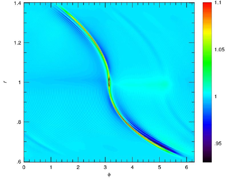
Figure 1: Density structure of the 2D standard model as generated by an embedded planet with $q=6\times 10^{-6}$ in a disk having the aspect ratio $H/r=0.05$. Shown is the configuration after $30\,T_{\mathrm{orb}}$. The density is scaled linearly.

To set the stage and illustrate the important physical effects, we first present the results of our simulations for the 2D standard case using the parameters according to Table 1. For the simulations in this section we used the RH2D code unless otherwise stated. Below, we will then discuss the variations from the standard model.

After the insertion of the planet, the planet’s gravitational disturbance generates two wakes, in the form of trailing spiral arms. The basic structure of the surface density, $\Sigma$, is shown in Fig. 1. As seen from the plot, the used damping procedure ensures that reflections by the radial boundaries are minimized. There is indication of vortex formation as can be seen by the additional structure in the right hand side of Fig. 1. Vortices induced by the planet occur for low viscosity disks and have been seen already in earlier simulations (see e.g. Li et al. 2005; de Val-Borro et al. 2006; Li et al. 2009). Here, we will not discuss this issue any further.

The relevant quantity to study the physical consequences of the interaction of the embedded planet with the ambient disk is the gravitational torque exerted on the planet by the disk. For that purpose it is very convenient to calculate the radial torque distribution per unit disk mass, $d\Gamma(r)/dm$, which we define here, following D’Angelo & Lubow (2010), through the definition of the total torque, $\Gamma_{\rm tot}$, acting on the planet

$$\Gamma_{\rm tot}=2\pi\int\frac{d\Gamma}{dm}(r)\,\Sigma(r)\,rdr\,.$$ (10)

Here, $d\Gamma(r)$ is the torque exerted on the planet by a disk annulus of width $dr$ located at the radius $r$ and having the mass $dm$. As $d\Gamma(r)/dm$ scales with the mass ratio squared and as $(H/r)^{-4}$, we rescale our results accordingly in units of

$$\left(\frac{d\Gamma}{dm}\right)_{0}=\Omega_{\mathrm{p}}^{2}(a_{\mathrm{p}})a_{\mathrm{p}}^{2}q^{2}\left(\frac{H}{a_{\mathrm{p}}}\right)^{-4},$$ (11)

where the index $p$ denotes that the quantities are evaluated at the location of the planet, which has the semi-major axis $a_{\mathrm{p}}$.

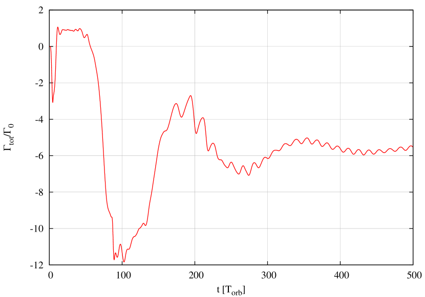
Figure 2: The total torque, $\Gamma_{\rm tot}$, in units of $\Gamma_{0}$ (see Eq. 12), acting on the planet vs. time for the 2D standard model. Shortly after insertion, the torque is positive and approximately constant between 10 and 40 orbits. At later times it saturates due to mixing of the material within the horseshoe region.

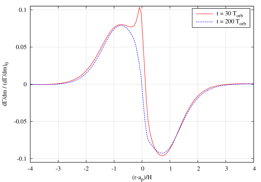
Figure 3: The radial torque density in units of $(d\Gamma/dm)_{0}$ (see Eq. 11) at 30 and 200 $T_{\mathrm{orb}}$ for the 2D standard model. The torque enhancement and spike near $r=1$ at $t=30\,T_{\mathrm{orb}}$ is due to the unsaturated corotation torque. At later times, here shown at $t=200\,T_{\mathrm{orb}}$, only the Lindblad contributions due to the spiral arms remain.

The time evolution of the total torque, $\Gamma_{\rm tot}$, is displayed in Fig. 2 for the first 500 orbits. The total torque is stated in units of

$$\Gamma_{0}=\Sigma_{0}\,\Omega_{\mathrm{p}}^{2}(a_{\mathrm{p}})a_{\mathrm{p}}^{4}q^{2}\left(\frac{H}{a_{\mathrm{p}}}\right)^{-2}\,.$$ (12)

In this simulation, the planetary potential has been ramped up during the first 5 orbits. After insertion of the planet the total torque becomes first positive and remains constant at this level for about 30 orbits. In this phase the co-orbital torque, in particular the horseshoe drag, is fully unsaturated and gives rise to a total positive torque. In our situation of an isothermal disk this comes about because of a non-vanishing vortensity gradient across the horseshoe region which generates in this case a strong positive corotation torque (Goldreich & Tremaine 1979). The vortensity, which is defined as vorticity divided by surface density, is here given by

$$\zeta=\frac{(\nabla\times\@vec{u})|_{z}}{\Sigma}\,.$$ (13)

As can be seen from this definition, for a constant $\Sigma$ disk the radial gradient of $\zeta$ is $\propto r^{-3/2}$, which leads to the strong vortensity-related torque. However, due to the different libration speeds, the material within the corotation region mixes and the gradients of potential vorticity and entropy are wiped out in the absence of viscosity (Balmforth & Korycansky 2001; Masset 2001). Consequently, the torques drop again, and oscillate on timescales on the order of the libration time towards a negative equilibrium value, which is given by the Lindblad torques generated by the spiral arms. This saturation of the vortensity-related torque related torque has been analyzed for example by Ward (2007) through an analyzes of streamlines within the horseshoe region for an inviscid disk, and later through two-dimensional hydrodynamic simulations by Masset & Casoli (2010); Paardekooper et al. (2011). The strength of the (positive) corotation torque depends strongly on the smoothing of the gravitational potential. For the chosen small $\epsilon=0.1$ this results in a positive total torque. For more realistic values of $\epsilon\approx 0.6-0.7$, $\Gamma_{\rm tot}$ will usually be negative, see Section 5.2.

To study the spatial origin of the torques we analyze the radial torque density for the standard model. In Fig. 3 the torque density $d\Gamma/dm$, according to Eq. 11 is displayed vs. radius in units of $(d\Gamma/dm)_{0}$. Two snapshots are displayed, one at $t=30\,T_{\mathrm{orb}}$ where the torque is fully unsaturated and one at $t=200\,T_{\mathrm{orb}}$ where the torque is saturated. We note, that for the torque calculation we use a tapering function near the planet to avoid contributions of material that is bound to the planet, or is so close to yield large torque fluctuations due to numerical discretization effects. We use the form as given in Crida et al. (2008) which reads

$$f(s)=\left[\exp\left(-\,\frac{\,s-r_{\mathrm{t}}}{0.1r_{\mathrm{t}}}\,\right)+1\right]^{-1}\,,$$ (14)

with a tapering length of $r_{\mathrm{t}}=0.8\,R_{\mathrm{H}}$. Here, $R_{\mathrm{H}}=(q/3)^{1/3}a_{\mathrm{p}}$ is the Hill radius of the planet. Such a tapering is particularly useful for massive planets that form a disk around them (Crida et al. 2009). Around lower mass planets, with ${\cal M}\lesssim 0.6$, circumplanetary disks do not form (Masset et al. 2006) and a large tapering is not required. Indeed, we found that for values of $r_{\mathrm{t}}$ in the range of $0.4-1.0R_{\mathrm{H}}$ there is not a large difference in the measured torques in equilibrium. For example, the variations of the total torque in Fig. 2 are less than $5\%$.

The torque density in the fully saturated phase, at $t=200\,T_{\mathrm{orb}}$ (Fig. 3, blue line), is positive inside of the planet and negative outside of the planet. The positive contribution of this Lindblad torque comes from the inner spiral arm, and the negative part from the outer one. The distribution at the earlier time, $t=30\,T_{\mathrm{orb}}$, shows an additional contribution and spike just inside of the planet. This part is due to the horseshoe drag which is subject to the described saturation process.

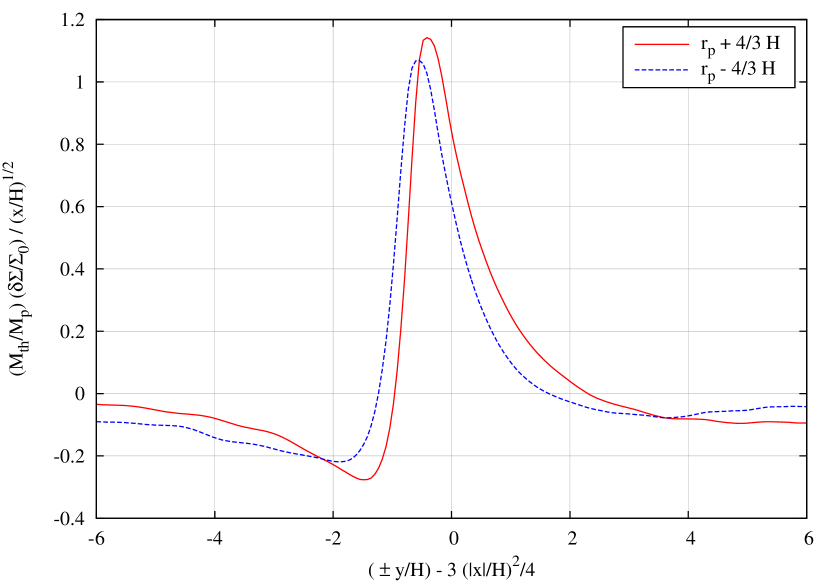
Figure 4: Normalized azimuthal density profile of the inner and outer wake at radial distances $\pm 4/3H$ away from the planet at 30 $T_{\mathrm{orb}}$ for the isothermal 2D standard model. The coordinates $x$ and $y$ refer to local Cartesian coordinates, see Eq. (15). The ’plus’ sign in the $x$-axis label refers to the blue curve at $r_{\mathrm{p}}-4/3H$, and the ’minus’ sign to the red curve at $r_{\mathrm{p}}+4/3H$. The upstream side of the wake is to the left for both curves.

To study the wake properties generated by the planet we use here a quasi-Cartesian local coordinate system centered on the planet to allow direct comparison to previous linear results. Specifically, we define

$$x=(r-r_{\mathrm{p}})\quad\mbox{and}\quad y=(\phi-\phi_{\mathrm{p}})r_{\mathrm{p}}\,.$$ (15)

In Fig. 4 the relative density perturbations for the inner and outer wakes are shown along the azimuth. They are displayed at a radial distance of $x=\pm 4/3H$ from the location of the planet. For the normalization of the perturbed density we define first the thermal mass of the planet

$$M_{\mathrm{th}}=\left(\frac{c_{s}^{3}}{G\Omega}\right)_{\mathrm{p}}=h^{3}\,M_{*}\,,$$ (16)

where the quantities have to be evaluated at the location of the planet. Then, the ratio of the planet mass to the thermal mass is given by

$$\frac{M_{\mathrm{p}}}{M_{\mathrm{th}}}=\frac{q}{h^{3}}={\cal{M}}^{3}\,.$$ (17)

Now, we follow Dong et al. (2011b) and scale $\delta\Sigma=\Sigma(\phi)-\Sigma_{0}$ by the planet mass (in units of $M_{\mathrm{th}}$) and normalize by $x/H$.

Due to the radial temperature variation and the cylindrical geometry, the inner and outer wake differ in their appearance. However, the general shape and magnitude is very similar to the linear results that have been obtained for the local shearing sheet model (see Goodman & Rafikov 2001; Dong et al. 2011b). Differences in the amplitude are presumably due to a different normalization. Because our results (in all simulations and with all codes) are consistently by factor of 3/2 larger than those of Dong et al. (2011b) we suspect that they might have used the normalization of $M_{\mathrm{th}}$ as given by Goodman & Rafikov (2001) which differs exactly by this factor. At the displayed distance from the planet the wake is expected to be in the linear regime, which results in a smooth maximum. For this reason we do not expect a large dependence on the numerical resolution. In the following, we will use only the outer wake to check for possible variations due to setup, numerical methods and resolution.

4 Testing numerics

To validate our results, and demonstrate that the FARGO-algorithm yields accurate results, we varied the numerical setup, and used several different codes on the same physical problem. In this Appendix we describe our studies in more detail.

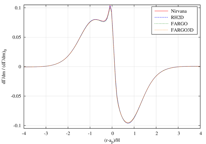
Figure 5: The radial torque density of the 2D standard-problem in units of $(d\Gamma/dm)_{0}$ at 30 $T_{\mathrm{orb}}$ for different codes at the standard resolution.

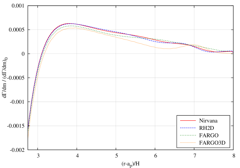
Figure 6: The radial torque density in units of $(d\Gamma/dm)_{0}$ at 30 $T_{\mathrm{orb}}$ for the standard setup for various code. This is enlargement of Fig. 5.

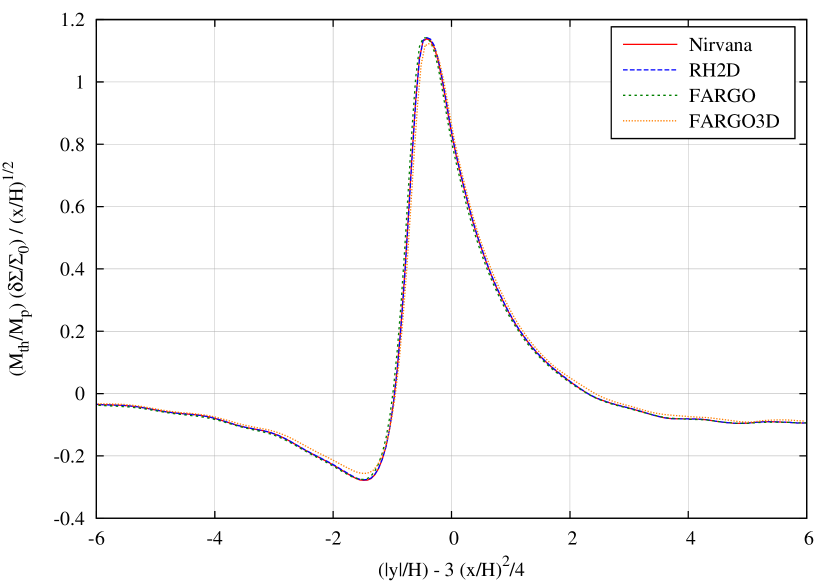
Figure 7: Normalized azimuthal density profile of the outer wake at the radius $r_{\mathrm{p}}+4/3H$ at 30 $T_{\mathrm{orb}}$ for different codes at the standard resolution.

4.1 Using different codes on the 2D standard model

To support our findings on the torque density and wake form and demonstrate the accuracy of the used codes, we ran the 2D standard model in the isothermal and the adiabatic version using all of the above codes. All use the FARGO-setup and are run in the same (standard) resolution. The isothermal results for the torque density are shown in Figs. 5 and 6, where the latter displays an enlargement of the first. Clearly, the results agree extremely well for the different codes. This includes the standard Lindblad torques as well a the detailed structure of the corotation torque. The FARGO3D code has been used in its 2D version for this test.

Recently, it has been shown by Dong et al. (2011b); Rafikov & Petrovich (2012) that the torque density $\Gamma(r)$ changes sign at a certain distance from the planet in contrast to the standard linear results (Goldreich & Tremaine 1979). Here, we show that this effect is reproduced in our simulations as well for all codes. In Fig. 6 we show that this reversal occurs at a distance $r_{\pm}\approx 3.1H$ away from the planet in good agreement with the linear results of Rafikov & Petrovich (2012). Again, all codes agree well on this feature, only FARGO3D shows small deviations.

The corresponding wake form at $x=r_{\mathrm{p}}+4H$ is displayed in Fig. 7. It is identical for all four cases, which shows the consistency and accuracy of the results and codes.

4.2 The FARGO treatment

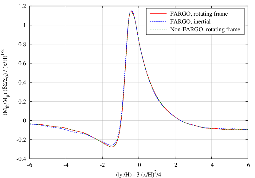
Figure 8: Normalized azimuthal density profile of the outer wake at the radius $r_{\mathrm{p}}+4/3H$ at 30 $T_{\mathrm{orb}}$ for the code RH2D using different timesteps and a non-rotating frame.

In Fig. 8 the wake form is analyzed for three different numerical usages of the FARGO-algorithm on the 2D standard setup. The first, red curve, corresponds to the standard reference case using a corotating coordinate system and the FARGO-algorithm. For the second, blue curve, the simulation has been performed in the inertial frame and using FARGO. In the mechanism of the algorithm, the quantities in each ring are first shifted according to the overall mean angular velocity of the ring, and then advected using the residual velocity (Masset 2000a). As a result, theoretically it should not matter whether the coordinate system is rotating or not. This is exactly what we find in our simulations, as the blue curve is very similar to the red one. Small differences can be produced by the planetary potential which is time dependent in the latter case, as the planet is moving, and lies at different locations with respect to the numerical grid. Also, the number of timesteps used until 30 $T_{\mathrm{orb}}$ are identical for two runs ($12,866$ steps). The third, green curve, corresponds to a model in the corotating frame without using the FARGO-algorithm. Because of the small timestep size in this case, over ten times more timesteps had to be used in this case ($137,750$ steps). Nevertheless, the wake form is identical. These runs indicate, that the FARGO-algorithm captures the physics of the system correctly. At the same time it comes with a much larger timestep and hence much reduced computational cost. This also applies to modern Riemann-solvers such as PLUTO, as shown in section 5.4.

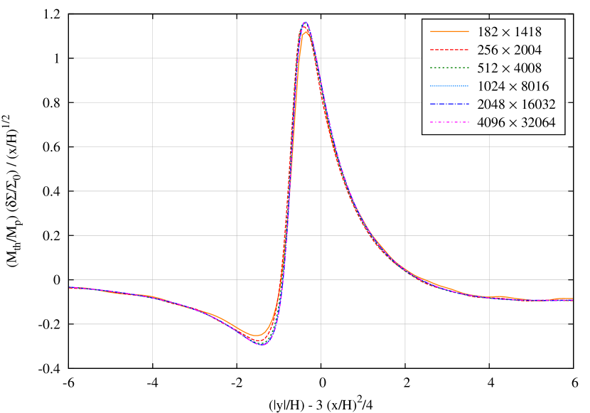
Figure 9: Normalized azimuthal density profile of the outer wake at the radius $r_{\mathrm{p}}+4/3H$ at 30 $T_{\mathrm{orb}}$ using the FARGO-code at different resolutions.

4.3 Testing numerical resolution

In order to estimate the effect of numerical resolution, we ran the 2D standard model using grid-sizes ranging from $182\times 1418$ all the way to $4096\times 32064$. This is equivalent to grid resolutions of $H/10$ to $H/256$. As shown in Fig. 9, the results are nearly identical at all resolutions. The first two, lower resolution cases have a slightly lower trough just in front of the wake and a smaller amplitude. As will be discussed later in Sect. 6, the results for the different resolutions are so similar because at this distance to the planet the wake is in the linear regime and has not steepened to a shock wave yet. The resolution requirements at the shock front will be analyzed in Sect. 6.

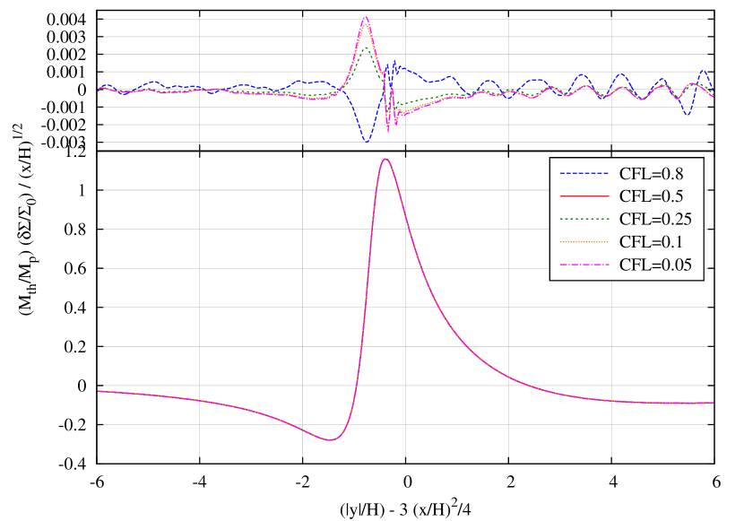
Figure 10: Normalized azimuthal density profile of the outer wake at the radius $r_{\mathrm{p}}+4/3H$ at 30 $T_{\mathrm{orb}}$ using the FARGO-code with different Courant-numbers (CFL). The physical setup differs slightly from the standard problem and is described in Sect. 4.4. In the upper panel the differences of the individual runs with respect to the standard, CFL=0.5, are displayed.

4.4 Testing timestep and stability

Finally, we would like to comment on possible timestep limitations due to the gravitational force generated by the planet. In our simulations we never found any unsteady evolution when using orbital advection. In contrast, the results of Dong et al. (2011b) indicate an unsteady behaviour for larger timesteps. They attribute possible instabilities to a violation of an additional gravity related timestep criterion and advocate using very small timesteps, which would render the FARGO-algorithm not applicable in very many cases.

To test specifically this statement we performed a suite of simulations on a setup very similar to that used by Dong et al. (2011b) in their Fig. 12. Due to the difficulty of RH2D and FARGO to use a Cartesian local setup we used here a computational domain exactly as before with a grid-size of $1024\times 8016$ which gives a resolution of 64 gridcells per scaleheight $H$. The planet mass is 1.33 $M_{\rm Earth}$, which is equivalent to a mass ratio $q=4\times 10^{-6}$ or $M_{\rm p}=3.2\times 10^{-2}M_{\rm th}$. For the potential smoothing we choose $\epsilon=0.08H$ which is yields a planetary potential nearly identical to that of Dong et al. (2011b). In Fig. 10 we display the results (using FARGO) for different timestep sizes as indicated by the corresponding Courant-number. The CFL = 0.5 case corresponds to our standard case. We made the timestep larger (CFL = 0.8) as well as smaller, down to CFL = 0.05. All cases yield identical results and do not show any sign of instability. In the upper panel the differences of the individual runs with respect to the standard, CFL=0.5, are displayed. The performed runs with the RH2D, FARGO and FARGO3D codes yield identical results, again with no signs of unsteady behaviour. Here, FARGO3D was run in the 2D version, both with the setup as indicated above and with the local setup of Tab. 3, with resolution $h/64$. For all our runs, past the first two orbits the wake profile at $x=1.33H$ has achieved convergence to better than the 1% level, regardless of the value of the timestep size. In Appendix B we re-analyze possible stability requirements in the presence of gravity and find indeed stability for the timestep sizes used with the FARGO-algorithm.

Note, that for these runs we switched off the physical viscosity completely. We find that the result for the wake displayed in Fig. 10 is in fact, due to the special scaling of the axes, identical to that of the standard problem as shown in the previous plots. Additionally, we have not seen any sign of unsteady behaviour. All of this indicates that our small value of the kinematic viscosity, $\nu=10^{-8}$ (in dimensionless units), is essentially negligible.

5 Using alternative setups

To illustrate how variations of individual properties of the standard model influence the outcome, we performed additional simulations which are described in this section.

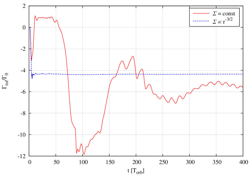
Figure 11: The total torque $\Gamma_{\rm tot}$, in units of $\Gamma_{0}$ (see Eq. 12), acting on the planet vs. time. Shown are the 2D standard model (red), and a globally isothermal case (blue), with a different density profile, such that the potential vorticity gradient vanishes.

5.1 Different radial stratification

As shown above, in the initial evolution after embedding the planet the total torque is positive due to a large positive horseshoe drag. The strength of this effect depends on the radial gradients of potential vorticity, entropy (for simulations with energy equation), and temperature (Baruteau & Masset 2012). To minimize this effect we present an additional, alternative setup where the gradients of potential vorticity (vortensity) and temperature vanish exactly. Hence, we chose a setup with a density gradient $\Sigma\propto r^{-3/2}$ and $T=\mathrm{const}$. The time evolution of the total torque for this model is displayed together with the standard case in Fig. 11. Clearly, after the short switch-on period of the planet mass, the total torque is negative and constant throughout the evolution. This demonstrates that for this density profile, $\Sigma\propto r^{-3/2}$, which resembles (coincidently) the minimum mass solar nebula, there is indeed no corotation torque present, and the flow settles directly to the Lindblad torque. The final value for the total Lindblad torque differs slightly for the two models due to the different gradients in density and temperature. We note that for this setup, with vanishing vortensity gradient, there are also no vortices visible during the initial evolution.

5.2 Comparing 2D and 3D simulations

Table 2: The numerical parameter for the 3D standard model

Parameter	Symbol	Value
smoothing radius	$r_{\mathrm{sm}}$	$0.25R_{\mathrm{H}}$
radial range	$R_{\mathrm{min}}$ – $R_{\mathrm{max}}$	$0.6$ – $1.4$
angular range	$\phi_{\mathrm{min}}$ – $\phi_{\mathrm{max}}$	$0$ – $2\pi$
meridional range	$\theta_{\mathrm{min}}$ – $\theta_{\mathrm{max}}$	$82\,^{\circ}$ – $90\,^{\circ}$
number of grid-cells	$N_{r}\times N_{\phi}\times N_{\theta}$	$256\times 2004\times 39$
spatial resolution	$\Delta r$	$H/16$
damping range at $R_{\mathrm{min}}$		$0.6$ – $0.7$
damping range at $R_{\mathrm{max}}$		$1.3$ – $1.4$

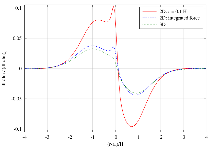
Figure 12: The radial torque density in units of $(d\Gamma/dm)_{0}$ at 30 $T_{\mathrm{orb}}$ for 2D and 3D simulations of the standard setup. The red curve corresponds to that in Fig. 3, the blue line to a 2D model with a vertical integrated gravitational force and the green to the 3D model (using NIRVANA).

Figure 13: Normalized azimuthal density profile of the outer wake at the radius $r_{\mathrm{p}}+4/3H$ at 30 $T_{\mathrm{orb}}$ for 2D and 3D simulations of the standard setup. The color coding is identical to Fig. 12.

The setup of the described standard case reduces the physical planet-disk problem to two dimensions. However, even though the disk may be thin, corrections are nevertheless expected due its finite thickness. We investigate this by performing full 3D simulations using the same physical setup as in the standard 2D model. The treatment of the inertial forces is outlined in Appendix C. The additional numerical parameters are listed in Table 2. The spatial extent and numerical resolution is identical to the 2D model. The initialization of the 3D density is chosen such that the surface density is constant throughout. In the vertical direction the density profile is initialized with a Gaussian profile as expected for vertically isothermal disks. The temperature is constant on cylinders. For the gravitational potential of the planet we chose the so called cubic-form (Kley et al. 2009) which is exact outside a smoothing radius $r_{\mathrm{sm}}$ and smoothed by a cubic polynomial inside of $r_{\mathrm{sm}}$. The advantage of this form lies in the fact that in 3D simulations the smoothing is required only numerically and the cubic potential allows us to have the exact potential outside a specified radius, here $r_{\mathrm{sm}}$. To calculate the torque the same tapering function (Eq. 14) as before has been used.

In Fig. 12 we show the normalized torque density $d\Gamma/dm$ for 2D simulations in comparison to a full 3D simulation using the same physical setup. Due to the finite vertical extent the torques of the 3D model are substantially smaller than for the corresponding 2D setup. As Müller et al. (2012) have shown recently, this discrepancy can be avoided by performing a suitable vertical averaging procedure of the gravitational force. Specifically, the force acting on each disk element in a 2D simulation is calculated from the projected force that acts in the midplane of the disk. Denoting the distance of the disk element to the planet with $s$, the force density (force per area) is given by

$$F_{\mathrm{p}}(s)=-\int\rho\frac{\partial\Psi_{\mathrm{p}}}{\partial s}\,dz=-GM_{\mathrm{p}}s\int\frac{\rho}{(s^{2}+z^{2})^{\frac{3}{2}}}\,dz\,,$$ (18)

where $\Psi_{\mathrm{p}}$ is the physical 3D potential generated by the planet. For the vertical density stratification a Gaussian density profile can be assumed for a vertically isothermal disk as a first approximation. However, the change of the vertical density as induced by the planet has to be taken into account. The results using this averaging prescription in an approximate way (Müller et al. 2012) is shown additionally in Fig. 12 by the blue curve. The overall behavior and magnitude is very similar to the full 3D results. For comparison, a 2D model using a fixed $\epsilon=0.7H$ (instead of $0.1H$ of the standard model) for $\Psi^{\mathrm{2D}}_{\mathrm{p}}$ yields similar amplitude as the full 3D model but a slightly different shape (see Fig. 14).

In Fig. 13 we show the corresponding wake profile for the 2D and 3D setup. For the 3D case, the surface density is obtained by integration along the $\theta$ direction at constant spherical radii, $R$. Here, the wake amplitude of the full 3D model is again reduced in contrast to the flat 2D case, with $\epsilon=0.1$. The 2D model using the integrated force algorithm yields here again a better agreement. The 3D results displayed in these plots have been obtained with NIRVANA, but usage of the new code FARGO3D yields identical results, as is demonstrated in Fig. 14.

Figure 14: The radial torque density in units of $(d\Gamma/dm)_{0}$ at 30 $T_{\mathrm{orb}}$ for the 3D and 2D simulations of the standard setup. Compared are two 3D simulations (using NIRVANA and FARGO3D) with a 2D simulation, using $\epsilon=0.7$.

These results demonstrate clearly, that the $\epsilon$-parameter in the 2D planetary potential ($\Psi^{\mathrm{2D}}_{\mathrm{p}}$) cannot be chosen arbitrarily small, but has to be on the order of the scale height $H$ of the disk. Near to the planet a reduction is required to account for the reduced thickness, see Müller et al. (2012). Hence, the value of $\epsilon=0.1\,H$ as chosen for the standard setup is too small to yield good agreement with vertically stratified disks, and serves here only as a numerical illustration to connect to previous linear and numerical results (Goodman & Rafikov 2001; Dong et al. 2011b). As shown by Müller et al. (2012) a value of $\epsilon=0.7\,H$ yields similar amplitudes to the 3D case, in particular for the Lindblad torque, see Fig. 14. However, as can be seen from the figure, for the $\epsilon$-potential the relative strengths of the inner an outer torques differ from the full 3D and the 2D vertically integrated case.

5.3 Using a quasi-local setup

To demonstrate the agreement of our simulations with previously published local results, e.g. by Dong et al. (2011b, a), we have changed the computational setup, which is listed briefly in Table 3. Despite the usage of cylindrical coordinates the setup is in fact identical to a model used by Dong et al. (2011b). The very small thickness $H$ of the disk and the small planet mass minimize curvature effects and make the problem more local. The nonlinearity parameter for this local model is ${\cal M}=0.32$, which is similar to the standard case. This quasi-local model has been run in a 2D and 3D setup using FARGO3D. The 3D case has been run again in spherical polar coordinates with the same spatial resolution as in the 2D setup of Table 3. For the gravitational smoothing a length of two grid-cells has been chosen, which is equivalent here to $\epsilon=0.06\,H$. For the 2D simulations we use RH2D and FARGO, while for the 3D simulations we use NIRVANA and FARGO3D. All these codes are based on the standard ZEUS-method and are enhanced with the FARGO-speedup, see Appendix A for details.

Table 3: The setup for the alternative quasi-local model. The parameters have been chosen according to Dong et al. (2011b).

Parameter	Symbol	Value
mass ratio	$q=M_{\rm p}/M_{*}$	$3.2\times 10^{-8}$
aspect ratio	$h=H/r$	$0.01$
nonlinearity parameter	${\cal M}=q^{1/3}/h$	$0.32$
potential smoothing	$\epsilon_{\mathrm{p}}$	$0.06H$
radial range	$r_{\mathrm{min}}$ – $r_{\mathrm{max}}$	$0.94$ – $1.06$
angular range	$\phi_{\mathrm{min}}$ – $\phi_{\mathrm{max}}$	$-0.32$ – $0.32$ rad
number of grid-cells	$N_{r}\times N_{\phi}$	$384\times 2048$
spatial resolution	$\Delta r$	$H/32$

Figure 15: The radial torque density in units of $(d\Gamma/dm)_{0}$. Compared is the standard setup with $q=6\times 10^{-6},h=0.05$ at 200 $T_{\mathrm{orb}}$ to the quasi-local model with $q=3.2\times 10^{-8},h=0.01$ at 30 $T_{\mathrm{orb}}$. The local calculation utilizes the FARGO3D-code in the 2D setup.

Figure 16: Normalized azimuthal density profile of the outer wake at the radius $r_{\mathrm{p}}+4/3H$ at 30 $T_{\mathrm{orb}}$. Compared is the standard setup with $q=6\times 10^{-6},h=0.05$ to the quasi-local model with $q=3.2\times 10^{-8},h=0.01$.

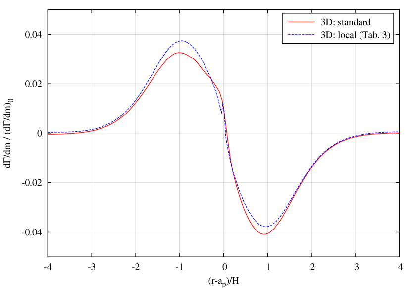
Figure 17: The radial torque density in units of $(d\Gamma/dm)_{0}$ for full 3D models. Compared is the standard setup with $q=6\times 10^{-6},h=0.05$ at 30 $T_{\mathrm{orb}}$ (using NIRVANA) to the quasi-local model with $q=3.2\times 10^{-8},h=0.01$ at 15 $T_{\mathrm{orb}}$ (using FARGO3D).

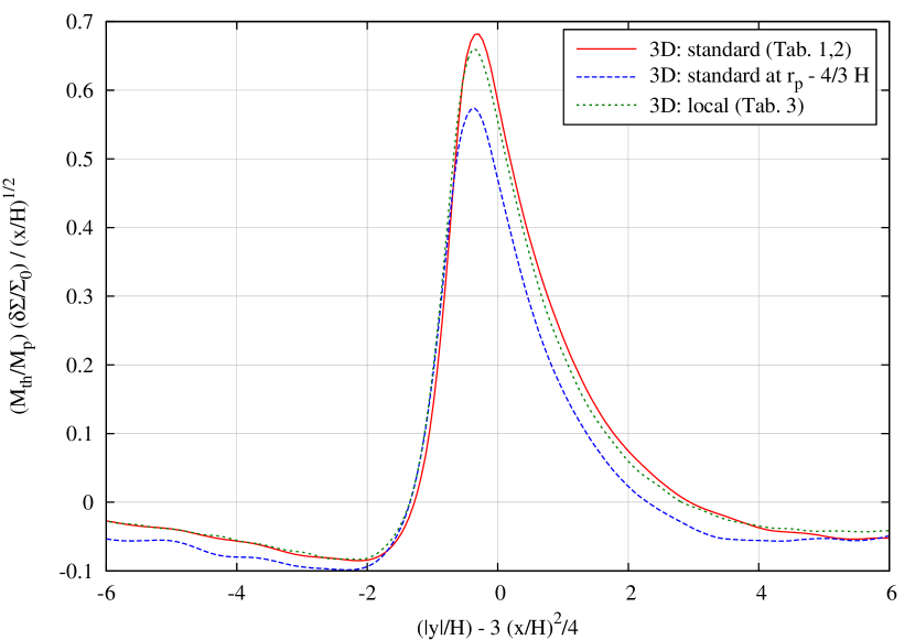
Figure 18: Normalized azimuthal density profile of the outer and inner wake at the radii $r_{\mathrm{p}}\pm 4/3H$ for full 3D models. Compared is the standard setup with $q=6\times 10^{-6},h=0.05$ at 30 $T_{\mathrm{orb}}$ for the outer and inner wake, to the quasi-local model with $q=3.2\times 10^{-8},h=0.01$ at 15 $T_{\mathrm{orb}}$, only at the outer wake.

In Fig. 15 we compare the torque density of the 2D standard model to the quasi-local model. In a local setup any corotation torques saturate very quickly, possibly due to the very small (quasi-periodic) domain in the angular direction. To match this condition, the standard model is shown here at $200T_{\mathrm{orb}}$ when the corotation torques have nearly saturated. The overall shape and magnitude of the two models is qualitatively in very good agreement, which supports the scaling with $(d\Gamma/dm)_{0}$. For the local models a symmetric shape with respect to the location of the planet is expected, while for standard model the outer torques are larger in magnitude. This can explain some differences.

In Fig. 16 we compare the wake form of the standard model (as shown in Figs. 4,13) to the more local alternative model for the 2D setup. The two curves agree very well indeed, despite the huge difference in parameters for the planet mass and the disk scale height. We attribute the small differences to curvature effects. We note that, due the local character of this setup, the curves for inner and outer wakes at $r_{\mathrm{p}}\pm 4/3$ look identical for the quasi-local model.

In Fig. 17 we compare the torque density of the 3D standard model to the 3D quasi-local model. As in the 2D case, now the overall shape and magnitude of the two models is again qualitatively in good agreement. The local model shows a symmetric shape with respect to the location of the planet, as expected. For both cases a similar reduction of amplitude in comparison to the 2D case is seen.

In Fig. 18 we compare the wake form of the standard model to the local alternative model for the full 3D setup. This time the two curves for the outer wake agree again very well, despite the huge difference in parameters. The profile for the inner wake of the standard model deviates from the outer wake as for the previous 2D setup. For the local model, inner and outer wake are again identical, as expected.

5.4 Adiabatic simulations

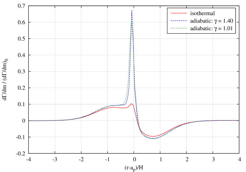
Figure 19: The radial torque density in units of $(d\Gamma/dm)_{0}$ (see Eq. 11) at 30 $T_{\mathrm{orb}}$ for the 2D standard model for an isothermal and adiabatic setup using $\gamma=1.01$ and $\gamma=1.40$. The units for $(d\Gamma/dm)_{0}$ and $H$ have been changed for the adiabatic runs, such that $H\rightarrow\gamma H$.

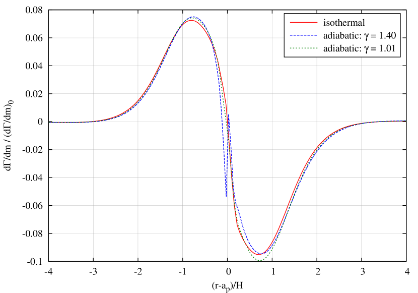
Figure 20: The radial torque density in units of $(d\Gamma/dm)_{0}$ (see Eq. 11) at 500 $T_{\mathrm{orb}}$ for the 2D standard model for an isothermal and adiabatic setup using $\gamma=1.01$ and $\gamma=1.40$. The units for $(d\Gamma/dm)_{0}$ and $H$ have been rescaled as in Fig. 19.

The assumption of isothermality is only satisfied approximately in protoplanetary disks. Because cooling times can be long, it maybe more appropriate to take into account the energy equation. To study the influence of the equation of state on the outcome, we performed purely adiabatic simulations, that solve the energy equation (Eq. 4) together with an ideal equation of state. The result of such an approach is presented in Fig. 19, where the radial torque density is displayed for the standard isothermal model together with two adiabatic models using $\gamma=1.4$ and $1.01$, respectively. The adiabatic results require rescaled units because the adiabatic sound speed is by a factor $\sqrt{\gamma}$ larger than the isothermal one. Hence, the pressure scale length is increased by the same factor, which enters (through $H$) the units for $(d\Gamma/dm)_{0}$ and $\Gamma_{0}$. Obviously, there is a huge difference in the horseshoe torque between isothermal and adiabatic runs, while the Lindblad contributions are similar, once correctly scaled. The adiabatic runs yield similar results for the two $\gamma$ values throughout. The strong torque enhancement in this adiabatic simulations comes from the entropy-related part of the corotation torque which is driven by a radial gradient of entropy across the horseshoe region (Baruteau & Masset 2008).

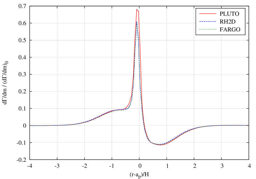
Figure 21: The radial torque density in units of $(d\Gamma/dm)_{0}$ (see Eq. 11) at 30 $T_{\mathrm{orb}}$ for the adiabatic standard model using an ideal equation of state with $\gamma=1.01$. Three different codes have been used, RH2D and FARGO are 2nd order upwind schemes and PLUTO is a Riemann solver.

This result is interesting because sometimes an isothermal situation is mimicked with an adiabatic simulation using a $\gamma$-value very close to unity. In particular, this may be required by Riemann solvers that do not allow to treat isothermal conditions. Our results show, that such an approach has to be treated very carefully, as shown already by Paardekooper & Mellema (2008). They argued that compressional heating near the planet plays an important role in determining the torques. Another reason lies in the fact that in an adiabatic situation the entropy is conserved along streamlines which is not the case for isothermal flows. Reducing the value of $\gamma$ even further yields the same results. In general, an adiabatic flow with $\gamma\rightarrow 1$ approaches truly isothermal flow only in the the case of a globally constant temperature.

After a few libration times the horseshoe region is well mixed, and the entropy and potential vorticity gradients across the horseshoe regions are wiped out. Hence, the horseshoe torques disappear and the Lindblad contributions remain. This situation is displayed in Fig.20 for an evolutionary time of $500$ orbits. Now, the isothermal model agrees well with the adiabatic one.

We have applied several codes on the adiabatic setup as well. In Fig. 21 we display the same results for the adiabatic situation using $\gamma=1.01$. Again, all codes agree very well, even though now the numerical methodology is vastly different as some use a second order upwind scheme (RH2D and FARGO) while PLUTO uses a Riemann-solver. Only very near to the planet the results differ slightly.

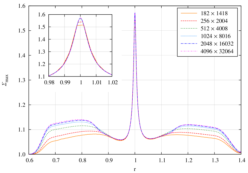
Figure 22: The maximum of the density in the spiral wake as a function of radius for the 2D isothermal standard model at 30 $T_{\mathrm{orb}}$. Different numerical resolutions are shown using FARGO.

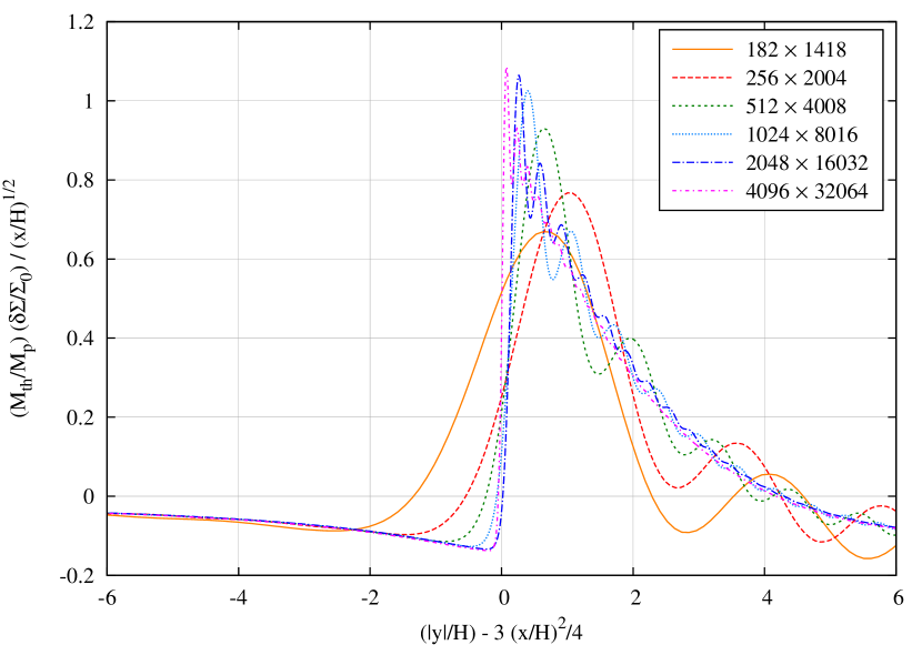
Figure 23: Normalized azimuthal density profile of the outer wake at the radii $r_{\mathrm{p}}+5H$ at 30 $T_{\mathrm{orb}}$ for the 2D isothermal standard model. Different numerical resolutions are shown.

6 Shock formation

For the damping of the wake it is important where the transition to a shock occurs. As a shock indicates a discontinuous change in the fluid variables, numerical codes often have difficulty to resolve the structure in detail. To analyze this, we plot in Fig. 22 the maximum density in the wake as a function of radius for various resolutions of the computational grid. At the radius of the planet the density obviously has its maximum and it drops on both sides. The previous curves for the wake profile have been taken near the minimum value of the density maximum. Here, all resolutions show an identical maximum of the wake amplitude. Hence, as we have demonstrated in Sect. 4.3, the form of the wake does not depend very strongly on resolution at a distance of $|x|=4/3H$.

Further away from the planet, beyond a distance $|x|\gtrsim 2H$ the curves begin to differ for the various resolutions. This is clearly an indication for non-convergence of the simulations. We attribute this to the formation of a shock wave. Indeed, at a distance $x_{\mathrm{s}}\approx 2H$ from the location of the planet the speed of the wake becomes supersonic with respect to the local Keplerian flow. The criterion as given by Goodman & Rafikov (2001) indicates for our nonlinearity parameter, ${\cal M}=0.36$, a shock formation at a distance of $\leavevmode\nobreak\ \approx 2.9H$ from the planet, consistent with our findings. At very high spatial resolutions, i.e. above a grid resolution of 64 grid-cells per scale height (1024$\times$8016), the curves begin to converge in the shock region. Far away from the planet, beyond $|x|\approx 6H$ ($r=1.3$) the damping action of the boundary condition begins to set in, and the curves coincide again.

In Fig. 23 the azimuthal density profile is shown at a radial location $r=r_{\mathrm{p}}+5H$ = 1.25. At this location the wake is expected to have turned into a shock wave. Due to the trailing nature of the wake we define the variable $y$ here slightly different as before through

$$y=(\phi-\phi_{\mathrm{p}})\,r\,.$$

From the figure it is obvious that the wake has turned into a shock at this location. At our standard resolution (256$\times$2004) there is no indication for a shock front. The overall form is very smooth with the presence of large oscillations behind the wake. With increasing numerical resolution the shock becomes better and better resolved, but only at the very highest resolution the wake turns into a discontinuous jump. The oscillations behind the front diminish and move closer to the front with increasing resolution. Numerical experiments show that these oscillations can be damped out by increasing the strength of viscosity. However, this smears out the shock front as well. It has been suggested that these oscillations are due to the used numerical scheme and occur for very weak shocks (Rein 2010).

7 Summary

Through a series of 2D and 3D simulations using different computational methods and codes we have explored in detail the numerical requirements for studies of the planet-disk problem. In our analysis we focus on the torque density acting on the planet and the structure of the wake generated by the planet.

With respect to the applicability of the fast orbital advection algorithm, FARGO, we have shown that it leads to consistent numerical results that agree extremely well with non-FARGO studies. The achievable gain in speed can be significant. For the setup used here we found a speed-up of more than a factor of 10. The method works well in the presence of embedded planets, does not show any signs of unsteady behavior, and can be applied in two or three spatial dimensions. As it is applicable in conjunction with magnetic fields as well, new possibilities with respect to numerical studies of turbulent accretion disks open up (Mignone et al. 2012).

Concerning the treatment of the gravitational potential of embedded planets, we extend previous studies (Masset 2002; Müller et al. 2012) to very low mass planets in extremely thin disks. We confirm that, for physical reasons, in 2D simulations the planetary potential has to be smoothed with about $\epsilon=0.6\,H$ – $0.7\,H$. Models where the gravitational force is obtained directly through a vertical integration yield always reasonable agreement with full 3D simulations. The usage of very small smoothing lengths below $\epsilon=0.6\,H$ in 2D simulations is not recommended, because then the forces in the vicinity of the planet are strongly overestimated, which results in an unphysical enhancement of the torque and too strong wakes.

Through a careful resolution study, we show that the smooth wake structure at distances smaller than about $2\,H$ of the planet can be resolved well, and consistently, already with very low resolution of 8 to 16 cells per scale height. The results are clearly converged for 32 grid-cells per $H$. For larger distances from the planet, the spiral wake turns into a shock wave and much higher resolution may be required. We found, that around a resolution of about 100 grid-cells per $H$ convergence can be achieved. Because this high resolution is only required near the spiral shocks, and the flow is relatively smooth outside, numerical methods that adaptively refine this crucial region may be the method of choice in the future.

For adiabatic flows we confirm earlier findings (Paardekooper & Mellema 2008) that the unsaturated horseshoe drag shows a strong deviation from the isothermal case. Using the appropriate scaling the adiabatic corotation torques are independent of $\gamma$ and do not converge to the isothermal case, even in the limit $\gamma\rightarrow 1$. Hence, the procedure of modelling the isothermal case with simulations of $\gamma$ close to unity, has to be treated with care. In the final saturated case, where all the corotation effects have been wiped out, isothermal and adiabatic results agree perfectly, once the correction to the sound speed has been applied.

In Appendix 4.3 we have shown that we do not find an additional timestep criterion due to the planetary potential and we also have not noticed any unstable evolution in the case of using the orbital advection. The question why in the simulations using the ATHENA-code instabilities occur (Dong et al. 2011b) may be connected to the treatment of orbital advection in that code (Stone & Gardiner 2010) which is apparently different from the implementation in the FARGO-code. One should also notice that in such simulations the conservative treatment of Coriolis forces is mandatory to properly conserve angular momentum (Kley 1998).

We have demonstrated that the planet-disk interaction problem may be regarded as a very good test to validate an implementation of orbital advection, because it admits a nearly analytic solution to which a code output can be compared. This is not the case for simulations of turbulent disks, where no such known solutions exist. We hope, that the presented results and comparison simulations may serve as a useful reference for other researcher in this field.

Appendix A The codes

For our comparison simulations we utilized the following codes:

NIRVANA: In its original (FORTRAN) version a ZEUS-like second order upwind scheme (Ziegler & Yorke 1997), with the option of fixed nested grids and magneto-hydrodynamics (MHD). It can be used in two or three dimensions and can use different coordinate systems. Recently, it has been improved to include radiative transport and the FARGO-treatment (Kley et al. 2009).

RH2D: A two-dimensional radiation hydrodynamics code for different coordinate systems, originally developed for treating the boundary layer in accretion disks (Kley 1989), and later adapted to the planet disk problem (Kley 1999).

FARGO: A two-dimensional, special purpose code for disk simulations that first featured the FARGO-algorithm (Masset 2000a). The code is publicly available at: http://fargo.in2p3.fr/, and has been used frequently in planet-disk and related simulations.

FARGO3D: A code based on similar algorithms as the standard FARGO-code, but aimed at being more versatile, as it includes Cartesian, cylindrical and spherical geometries, in one, two or three dimensions, with arbitrary grid limits. Its hydrodynamical core has been written from scratch, and it includes an MHD solver based on the method of characteristics and constrained transport. It is parallelized using the Message Passing Interface (MPI) and a slab domain decomposition. It is intended in a nearby future to run distinctly on clusters of CPUs or GPUs, and it will be made publicly available as the successor of the FARGO-code.

PLUTO: A multi-dimensional Riemann-solver based code for MHD flows (Mignone et al. 2007), which can be used in the purely hydrodynamic setup as well. Additionally, it has been empowered recently by the FARGO-algorithm (Mignone et al. 2012). PLUTO is also freely available at: http://plutocode.ph.unito.it.

The first 3 codes in the list have been used and described in an earlier code comparison project on the planet-disk problem (de Val-Borro et al. 2006). There, more massive planets of Neptune and Jupiter mass embedded in viscous and inviscid disks have been studied for a large number of codes, and the focus was on the gap structure of the disk and the total torques have been analyzed.

Appendix B Timestep limitation in the presence of gravity

Numerically, we expect that possibly gravity might cause problems if, due to the gravitational acceleration $g$, a parcel of material travels more than about half a gridcell of length $\Delta x$ in one timestep $\Delta t$. This requires the additional gravitational criterion

$$\Delta t_{\mathrm{G}}\leq\left(\frac{\Delta x}{g}\right)^{1/2}\,.$$ (19)

Using now the smoothed planetary potential of Eq. (6) we find that the maximum force is given by

$$g_{\mathrm{max}}=\frac{GM_{\mathrm{p}}}{\epsilon^{2}}\,k$$ (20)

with $k=2/3^{3/2}\approx 0.4$. To obtain the strongest limitation on $\Delta t$ we substitute $g_{\mathrm{max}}$ in Eq. (19) and obtain

$$\Delta t_{\mathrm{G}}\leq\Omega_{\mathrm{K}}^{-1}\,{\cal M}^{-1/2}\,\left(\frac{2\Delta x\,\epsilon^{2}}{k\,H^{3}}\right)^{1/2}\,.$$ (21)

We compare this limit now to the regular Courant condition when using orbital advection which is given by

$$\Delta t_{\mathrm{C}}=\frac{\Delta x}{c_{\mathrm{s}}}\,,$$ (22)

and find

$$\frac{\Delta t_{\mathrm{G}}}{\Delta t_{\mathrm{C}}}={\cal M}^{-1/2}\left(\frac{2\epsilon^{2}}{kH\Delta x}\right)^{1/2}\,.$$ (23)

If there should be no additional timestep limitation generated by the gravity then this ratio should be larger than one. Writing now for the grid resolution $\Delta x=H/N$ we obtain finally that

$$N\geq\frac{k}{2}\,\frac{H^{2}}{\epsilon^{2}}\,{\cal M}$$ (24)

for stability. With $k=0.4$, $\epsilon=0.1H$, and ${\cal M}=0.36$ we find for the necessary resolution $N\approx 10$. This is indeed fulfilled even for our lowest resolution. We point out that this limit formally only applies to flows without pressure (dust). If around the planet the envelope is hydrostatic, no additional criterion is required. Switching on the planetary potential slowly will ensure stability throughout the evolution as will an initial atmosphere around the planet (Duffell & MacFadyen 2012).

Appendix C The 3D hydrodynamic equations in a rotating frame

For reference we state here the 3D hydrodynamic equations in a rotating coordinate frame. In a coordinate system rotating with the (constant) angular velocity ${\bf\Omega}$, omitting pressure terms, any external forces (eg. gravitation) and viscosity, the momentum equation reads:

$$\frac{\partial{\bf u}}{\partial t}+{\bf u}\nabla{\bf u}=-2{\bf\Omega}\times{\bf u}+\frac{1}{2}\nabla\left[({\bf\Omega}\times{\bf r})^{2}\right]$$ (25)

We now use spherical polar coordinates ($r,\varphi,\theta$), where $r$ is the radial coordinate, $\varphi$ is the azimuthal angle, and $\theta$ is the usual polar coordinate measured from the $z-$axis. NOTE, that we use in this Appendix the same symbol $r$ for the spherical radial coordinate. For rotation around the $z$-axis, ${\bf\Omega}=\Omega{\bf e}_{z}$, the individual equations are:

$$\frac{\partial u_{r}}{\partial t}+{\bf u}\nabla u_{r}=\frac{1}{r}\left(u_{\varphi}^{2}+u_{\theta}^{2}\right)+r\Omega^{2}\sin^{2}\theta+2u_{\varphi}\Omega\sin\theta$$ (26)

$$\frac{\partial u_{\varphi}}{\partial t}+{\bf u}\nabla u_{\varphi}=-\frac{u_{r}u_{\varphi}}{r}-\frac{u_{\theta}u_{\varphi}\cot\theta}{r}-2\Omega\left(\sin\theta u_{r}+\cos\theta u_{\theta}\right)$$ (27)

$$\frac{\partial u_{\theta}}{\partial t}+{\bf u}\nabla u_{\theta}=-\frac{u_{r}u_{\theta}}{r}+\frac{u_{\varphi}^{2}\cot\theta}{r}+2\Omega u_{\varphi}\cos\theta+\Omega^{2}r\sin\theta\cos\theta$$ (28)

Introducing the angular velocity $\omega$ through

$$u_{\varphi}=r\sin\theta\,\omega$$ (29)

we may write for the three equations (26 - 28)

$$\frac{\partial u_{r}}{\partial t}+{\bf u}\nabla u_{r}=\frac{u_{\theta}^{2}}{r}+r\sin^{2}\theta\left(\omega+\Omega\right)^{2}$$ (30)

$$\frac{\partial u_{\varphi}}{\partial t}+{\bf u}\nabla u_{\varphi}=-\left(\omega+2\Omega\right)\left(\sin\theta u_{r}+\cos\theta u_{\theta}\right)$$ (31)

$$\frac{\partial u_{\theta}}{\partial t}+{\bf u}\nabla u_{\theta}=-\frac{u_{r}u_{\theta}}{r}+r\sin\theta\cos\theta\left(\omega+\Omega\right)^{2}$$ (32)

One sees that in the radial and meridional ($\theta$) momentum equation only the centrifugal part ($\omega+\Omega$) and in the angular momentum ($\varphi$) equation only the Coriolis term ($2\Omega$) occurs.

C.1 Conservative treatment of Coriolis Terms in Angular Momentum equation

Defining the total specific angular momentum

$$h_{t}=r^{2}\sin^{2}\theta\left(\omega+\Omega\right)$$ (33)

and using the continuity equation (in 3D) we may write for the angular momentum equation (31)

$$\frac{\partial\rho h_{t}}{\partial t}+\nabla\cdot\left(\rho h_{t}{\bf u}\right)=0$$ (34)

Expanding $h_{t}$ this may be written:

$$\frac{\partial\left[\rho r\sin\theta\left(u_{\varphi}+r\Omega\sin\theta\right)\right]}{\partial t}+\nabla\cdot\left[\rho r\sin\theta\left(u_{\varphi}+r\Omega\sin\theta\right){\bf u}\right]=0$$ (35)

The validity of this last equation (35) can be easily checked by expanding the terms and make use of the continuity equation. Then one arrives at the equation (31). In a numerical method that evolves $u_{\varphi}$ the equation (35) should be used to solve the angular momentum transport conservatively.

Appendix D Comparing to linear results

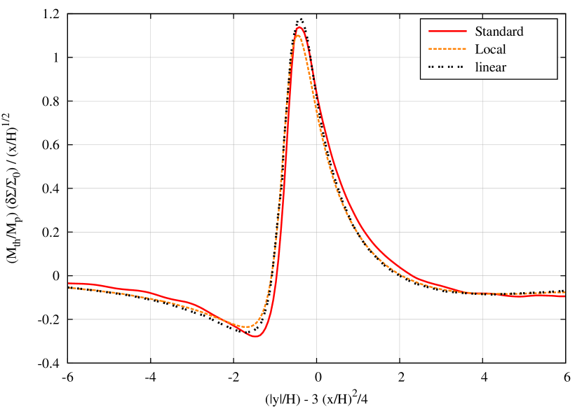
Figure 24: Normalized azimuthal density profile of the outer wake at the radius $r_{\mathrm{p}}+4/3H$ at 30 $T_{\mathrm{orb}}$. Compared is the standard setup with $q=6\times 10^{-6},h=0.05$ and the quasi-local model with $q=3.2\times 10^{-8},h=0.01$ to the linear theoretical results of Goodman & Rafikov (2001).

After submission of the original manuscript, Ruobing Dong generously supplied us with the data of the linear results of Goodman & Rafikov (2001). In Fig. 24 we compare their data to our results for the 2D simulations using the standard setup of Tab. 1 and the quasi-local setup of Tab. 3. The overall agreement of our full nonlinear results with the linear case is very good. The small differences between the results are comparable to what Dong et al. (2011b) found in their study. Please note, that their vertical scaling differs by a factor of 3/2.

References

- Balmforth & Korycansky (2001) Balmforth, N. J. & Korycansky, D. G. 2001, MNRAS, 326, 833
- Baruteau & Masset (2008) Baruteau, C. & Masset, F. 2008, ApJ, 672, 1054
- Baruteau & Masset (2012) Baruteau, C. & Masset, F. 2012, in Tidal effects in Astronomy and Astrophysics, Lecture Notes in Physics, to be published
- Crida et al. (2009) Crida, A., Baruteau, C., Kley, W., & Masset, F. 2009, A&A, 502, 679
- Crida et al. (2008) Crida, A., Sándor, Z., & Kley, W. 2008, A&A, 483, 325
- D’Angelo & Lubow (2010) D’Angelo, G. & Lubow, S. H. 2010, ApJ, 724, 730
- de Val-Borro et al. (2006) de Val-Borro, M., Edgar, R. G., Artymowicz, P., et al. 2006, MNRAS, 370, 529
- Dong et al. (2011a) Dong, R., Rafikov, R. R., & Stone, J. M. 2011a, ApJ, 741, 57
- Dong et al. (2011b) Dong, R., Rafikov, R. R., Stone, J. M., & Petrovich, C. 2011b, ApJ, 741, 56
- Duffell & MacFadyen (2012) Duffell, P. C. & MacFadyen, A. I. 2012, ApJ, 755, 7
- Gardiner & Stone (2008) Gardiner, T. A. & Stone, J. M. 2008, Journal of Computational Physics, 227, 4123
- Goldreich & Tremaine (1979) Goldreich, P. & Tremaine, S. 1979, ApJ, 233, 857
- Goodman & Rafikov (2001) Goodman, J. & Rafikov, R. R. 2001, ApJ, 552, 793
- Kley (1989) Kley, W. 1989, A&A, 208, 98
- Kley (1998) Kley, W. 1998, A&A, 338, L37
- Kley (1999) Kley, W. 1999, MNRAS, 303, 696
- Kley et al. (2009) Kley, W., Bitsch, B., & Klahr, H. 2009, A&A, 506, 971
- Korycansky & Papaloizou (1996) Korycansky, D. G. & Papaloizou, J. C. B. 1996, ApJS, 105, 181
- Li et al. (2005) Li, H., Li, S., Koller, J., et al. 2005, ApJ, 624, 1003
- Li et al. (2009) Li, H., Lubow, S. H., Li, S., & Lin, D. N. C. 2009, ApJ, 690, L52
- Masset (2000a) Masset, F. 2000a, A&AS, 141, 165
- Masset (2000b) Masset, F. S. 2000b, in Astronomical Society of the Pacific Conference Series, Vol. 219, Disks, Planetesimals, and Planets, ed. G. Garzón, C. Eiroa, D. de Winter, & T. J. Mahoney, 75
- Masset (2001) Masset, F. S. 2001, ApJ, 558, 453
- Masset (2002) Masset, F. S. 2002, A&A, 387, 605
- Masset & Casoli (2009) Masset, F. S. & Casoli, J. 2009, ApJ, 703, 857
- Masset & Casoli (2010) Masset, F. S. & Casoli, J. 2010, ApJ, 723, 1393
- Masset et al. (2006) Masset, F. S., D’Angelo, G., & Kley, W. 2006, ApJ, 652, 730
- Mignone et al. (2007) Mignone, A., Bodo, G., Massaglia, S., et al. 2007, ApJS, 170, 228
- Mignone et al. (2012) Mignone, A., Flock, M., Stute, M., Kolb, S. M., & Muscianisi, G. 2012, A&A, in press
- Müller et al. (2012) Müller, T. W. A., Kley, W., & Meru, F. 2012, A&A, 541, A123
- Paardekooper et al. (2010) Paardekooper, S.-J., Baruteau, C., Crida, A., & Kley, W. 2010, MNRAS, 401, 1950
- Paardekooper et al. (2011) Paardekooper, S.-J., Baruteau, C., & Kley, W. 2011, MNRAS, 410, 293
- Paardekooper & Mellema (2008) Paardekooper, S.-J. & Mellema, G. 2008, A&A, 478, 245
- Rafikov & Petrovich (2012) Rafikov, R. R. & Petrovich, C. 2012, ApJ, 747, 24
- Rein (2010) Rein, H. 2010, PhD thesis, University of Cambridge, ArXiv:1012.0266
- Stone & Gardiner (2010) Stone, J. M. & Gardiner, T. A. 2010, ApJS, 189, 142
- Ward (2007) Ward, W. R. 2007, in Lunar and Planetary Institute Science Conference Abstracts, Vol. 38, 2289
- Ziegler & Yorke (1997) Ziegler, U. & Yorke, H. W. 1997, Computer Physics Communications, 101, 54