Gravity Without Curved Spacetime: A Simple Calculation

Abstract

Classical-particle trajectories are calculated for the static Einstein universe without requiring that the 3-space be closed and curved. Freely-moving test particles are found to return to their starting positions because of strong gravitational-field effects. Possible implications for the underlying (quantum) theory of gravity are briefly discussed.

I Introduction

In the decades leading up to the construction of the standard model of elementary particle physics, the idea was explored that gravity could also be viewed as a (spin–2) gauge field theory in Minkowski spacetime. A selection of original articles/lectures is given in Refs. Kraichnan1955 ; Gupta1957 ; Thirring1961 ; Feynman1963 ; Weinberg1965 ; Deser1970 ; Veltman1976 and a selection of related textbook discussions in Refs. Feynman1964 ; Weinberg1972 ; MTW1973 .

The conclusion reached was that there is no fundamental difference between this flat-spacetime gauge-field-theory point of view and the standard geometric point of view (the one adopted by Einstein Einstein1916 ; Einstein1917 ). See, e.g., Sec. 8.3 of Ref. Feynman1963 and Box 18-1 of Ref. MTW1973 .

However, the naive question arises as to how the flat-spacetime approach would be able to describe, for example, a closed cosmological model. Veltman and the present author addressed this puzzle some time ago KlinkhamerVeltman1992 but did not reach a definite conclusion, because two contradictory results were obtained for the particle trajectories. Now, this contradiction has been resolved with the realization that the first of these results does not apply globally, whereas the second does.

We describe the outcome of this simple (and even trivial) calculation in Secs. II–V. At the end of this article, in Sec. VI, we point out that the result may be especially relevant if gravity is not fundamental but emergent.

II Gravity

As explained in the Introduction, the starting point is the suggestion Kraichnan1955 ; Gupta1957 ; Thirring1961 ; Feynman1963 ; Weinberg1965 ; Deser1970 ; Veltman1976 that gravity is a non-Abelian gauge field theory of a massless spin–2 field $h_{\mu\nu}(x)$ defined over flat Minkowski spacetime, just as the electromagnetic and strong interactions of the standard model are non-Abelian gauge field theories of spin–1 fields over Minkowski spacetime. In short, this description of gravity does not rely on the curved-spacetime concept.

Purely for convenience, define

$$g_{\mu\nu}(x)\equiv\eta_{\mu\nu}+h_{\mu\nu}(x)\,,$$ (1a)

where $$\eta_{\mu\nu}$$ is the Minkowski metric, here taken as

$$\eta_{\mu\nu}=\text{diag}(-1,\,-1,\,-1,\,+1)\,.$$ (1b)

A finite gauge transformation with parameters $\xi^{\kappa}(x)$ then transforms the spin–2 field $h_{\mu\nu}(x)$ contained in $g_{\mu\nu}(x)$ and a generic scalar field $\phi(x)$ as follows:

$$g_{\mu\nu}\big{(}x\big{)} \rightarrow \frac{\partial\xi^{\kappa}}{\partial x^{\mu}}\frac{\partial\xi^{\lambda}}{\partial x^{\nu}}\;g_{\kappa\lambda}\big{(}\xi(x)\big{)}\,,$$ (2a)

$$\phi\big{(}x\big{)} \rightarrow \phi\big{(}\xi(x)\big{)}\,.$$ (2b)

For the gravitational coupling of matter, gauge invariance effectively plays the role of the equivalence principle (cf. the last paragraph of Sec. 13 in Ref. Veltman1976 ). In fact, the invariant action (units $8\pi G_{N}=c=1$) reads

$$A=\int_{\mathbb{R}^{4}}d^{4}x\;\big{[}-\textstyle{\frac{1}{2}}\,\sqrt{g(x)}\,R(x)+\sqrt{g(x)}\,\mathcal{L}_{m}(x)\big{]},$$ (3)

with the density $g(x)$ given by the determinant of the $4\times 4$ matrix (1a) and the kinetic term $R$ equal to the Ricci “curvature” scalar in terms of the “metric” (1a). Note that the spacetime integral in (3) is always over $\mathbb{R}^{4}$.

The standard geometric point of view (developed by Einstein Einstein1916 ) is that there exist rigid measuring-rods and perfect standard-clocks in a curved space-time with line-element $ds^{2}=g_{\mu\nu}\,dx^{\mu}dx^{\nu}$. The alternative point of view (discussed by Feynman Feynman1963 , for example) is that the rods and clocks are deformed by a gravitational field $h_{\mu\nu}(x)$ defined over Minkowski spacetime. Feynman Feynman1963 and Misner–Thorne–Wheeler MTW1973 , amongst others, conclude that there are no important differences between these two points of views.

Expanding on these somewhat abstract discussions, we adopt a pragmatic approach and consider the trajectories of a classical test particle, in particular, the paths in a “closed” universe.

III Equation of motion

As pointed out by Einstein and Grommer (1927), it is possible to obtain the motion of a classical particle already from the gravitational field equations; see, e.g., Sec. 20.6 of Ref. MTW1973 and Sec. 11.1 of Ref. AdlerBazinSchiffer1975 for further discussion and references. A simple derivation of the equation of motion of a classical test particle with position $x_{p}$ then starts from energy-momentum conservation,

$$T^{\mu\nu}_{\phantom{\mu\nu};\nu}=0\,.$$ (4)

Consider dust particles with

$$T^{\mu\nu} = \rho_{0}(x)\,u^{\mu}(x)u^{\nu}(x)\,,$$ (5a)

$$u^{\mu} = \frac{dx^{\mu}}{ds}\,,\quad u^{\mu}u_{\mu}=1\,.$$ (5b)

It now follows that AdlerBazinSchiffer1975

$$\frac{d^{2}x_{p}^{\mu}}{ds^{2}}+\Gamma^{\mu}_{\kappa\lambda}(x_{p})\,\frac{dx_{p}^{\kappa}}{ds}\frac{dx_{p}^{\lambda}}{ds}=0\,,$$ (6a)

with the standard affine connection given in terms of the “metric” (1a), its inverse, and its derivatives,

$$\Gamma^{\mu}_{\kappa\lambda}\equiv\frac{1}{2}\,g^{\mu\nu}\,\left(\frac{\partial g_{\nu\kappa}}{\partial x^{\lambda}}+\frac{\partial g_{\nu\lambda}}{\partial x^{\kappa}}-\frac{\partial g_{\kappa\lambda}}{\partial x^{\nu}}\right)\,.$$ (6b)

The equation of motion (6a) is better known as the “geodesic equation,” here with quotations marks because we do not adopt a geometric point of view (or, at least, do not start from it).

Equation (6a) is form-invariant under gauge transformations,

$$g_{\mu\nu}(x) \rightarrow \frac{\partial\xi^{\kappa}}{\partial x^{\mu}}\frac{\partial\xi^{\lambda}}{\partial x^{\nu}}\;g_{\kappa\lambda}(\xi)\,,$$ (7a)

$$x^{\mu}_{p} \rightarrow \xi^{\mu}(x_{p})\,,$$ (7b)

as long as the gauge parameter $\xi^{\kappa}=\xi^{\kappa}(x)$ is an invertible function.

IV RW Universe: $\boldsymbol{k=1}$ case

For definiteness, consider a specific gravitational background field corresponding to the Robertson-Walker (RW) metric AdlerBazinSchiffer1975 ; RobertsonNoonan1968 with constant positive “curvature” of the spatial hypersurfaces ($k=1$ in the standard terminology). With Cartesian coordinates $x^{i}$ of the 3-space and the cosmic scale factor $a=a(t)$, the gravitational background field (1a) is given by

$$g_{\mu\nu}(x^{1},\,x^{2},\,x^{3},\,t) = \begin{pmatrix}&&&\;\;\;0\\ &-a(t)^{2}\,\widetilde{g}_{ij}(x)&&\;\;\;0\\ &&&\;\;\;0\\ 0&0&0&\;\;\;1\end{pmatrix}\,,$$ (8a)

$$\widetilde{g}_{ij}(x^{1},\,x^{2},\,x^{3}) = \left(\frac{1}{1+k\,|\vec{x}|^{2}/4}\right)^{2}\;\delta_{ij}\,,$$ (8b)

$$k = 1\,.$$ (8c)

There are no singularities in (8) and one coordinate patch suffices for $|\vec{x}|<\infty$. Note that the spatial coordinates $x^{i}$ are dimensionless and the cosmic scale factor $a(t)$ has the dimension of length, just as the cosmic time coordinate $t$ (recall $c=1$).

It is, then, easy to evaluate the equation of motion (6a) using

$$\Gamma^{i}_{oj}=\frac{\dot{a}}{a}\;\delta^{i}_{j}\,,\quad\Gamma^{0}_{ij}=\dot{a}\,a\;\widetilde{g}_{ij}\,,\quad\Gamma^{i}_{jk}=\widetilde{\Gamma}^{i}_{jk}\,,$$ (9)

where the overdot stands for differentiation with respect to $t$ and $\widetilde{\Gamma}^{i}_{jk}$ is the 3-dimensional version of (6b) for the metric (8b). The results for the 3-dimensional trajectories ($du^{2}=\widetilde{g}_{ij}\,dx^{i}dx^{j}$) are as follows:

$$\frac{d^{2}x^{i}}{du^{2}}+\widetilde{\Gamma}^{i}_{jk}\,\frac{dx^{j}}{du}\frac{dx^{k}}{du}=0\,,$$ (10a)

$$\left(\frac{dt}{du}\right)^{2}=a^{2}+\text{const}\,.$$ (10b)

It suffices for our purpose to consider the static Einstein universe Einstein1917 with a pressureless perfect fluid as matter component and a cosmological constant $\Lambda>0$ (units $8\pi G_{N}=c=1$):

$$a = 1/\sqrt{\Lambda}\,,$$ (11a)

$$\rho_{m} = 2\,\Lambda\,,$$ (11b)

$$P_{m} = 0\,,$$ (11c)

which solves the reduced Einstein field equations, i.e., the standard Friedmann equations obtained by inserting the expressions (9). [A similar discussion holds for the global de Sitter metric (cf. Sec. 16.3 of Ref. RobertsonNoonan1968 ), which is also given by (8) but now with the time-dependent scale factor $a(t)=\sqrt{3/\Lambda}\,\cosh(\sqrt{\Lambda/3}\;t)$.]

From (10b) and (11a), we have $u\propto t$, depending on the initial velocity of the particle, and we only need to solve for the 3-dimensional orbits from (10a).

V Orbits in flat space

Consider, first, the 2-dimensional case by taking the $x^{3}=0$ slice of the space manifold $\mathbb{R}^{3}$. Next, change the remaining two coordinates as follows:

$$\theta = \pi-2\,\arctan\left(\frac{\sqrt{(x^{1})^{2}+(x^{2})^{2}}}{2}\right)\,,$$ (12a)

$$\phi = \arctan\left(\frac{x^{2}}{x^{1}}\right)\,,$$ (12b)

which gives the following expression for the 2-dimensional metric:

$$a^{2}\,\widetilde{g}_{ij}\,dx^{i}dx^{j} = a^{2}\,\big{(}d\theta^{2}+\sin^{2}\theta\,d\phi^{2}\big{)}\,,$$ (12c)

where the indices $i,j$ are summed over $1$ and $2$. From the expression (12c) we are led to the following mathematical trick: the 2-dimensional gravitational field from (8b) can be interpreted as the metric on a 2-sphere with radius $a$. See Fig. 2, where $r$ is the radial coordinate from the point O in the plane and $\phi$ (not shown) is the azimuthal angle.

Figure 1: Coordinates for the physical plane and the auxiliary sphere, see main text.

Figure 2: Mathematical construction of the particle trajectories in the plane, see main text.

It is now easy to obtain the orbits in the flat 2-dimensional space RobertsonNoonan1968 : they are simply the projections of great circles on the sphere (each with a pole $\text{N}^{\prime}$ having spherical coordinates $\theta=\alpha$, $\phi=\beta$; see Fig. 2). The resulting orbits in the plane turn out to be circles with the following center positions and radii:

$$\big{(}r,\,\phi\big{)}_{\text{center}} = \big{(}2\,a\,\tan\alpha,\,\beta\big{)}\,,$$ (13a)

$$l_{\text{radius}} = \frac{2\,a}{\cos\alpha}\,.$$ (13b)

A “straight” path along the $x^{2}$ axis, for example, is obtained by considering a particular great circle in Fig. 2, which passes through O (i.e., $\alpha=\pi/2$) and is traversed many times in the same direction. The corresponding particle motion in the plane (i.e., the real space according to our point of view) then always passes O from the same direction, because the path “closes at infinity,” where $\widetilde{g}_{ij}=0$. Indeed, consider a great circle with $\alpha=\pi/2-\epsilon$ and let $\epsilon\to 0^{+}$. In the plane, this gives a path along the $x^{2}$ axis closed by a particular semi-circle “at infinity” (the other semi-circle occurs for $\epsilon\to 0^{-}$). The behavior is shown in Fig. 3, where the circle segments in the plane get closer and closer to the $x^{1}=0$ line as $\alpha$ increases towards the value $\pi/2$.

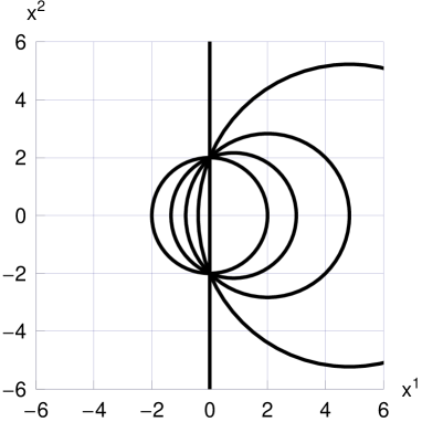
Figure 3: Selected particle trajectories in the static Einstein universe (11) with $\Lambda=1$. These trajectories can be obtained mathematically by projecting great circles with polar angle $\alpha$ $=$ $(0,\,1,\,2,\,3,\,4-0^{+})$ $\times$ $\pi/8$ as defined in Fig. 2 or by directly solving the equation of motion (10a) with appropriate boundary conditions. Further trajectories are obtained by reflection $x^{1}\to-x^{1}$.

Let us emphasize that the particle trajectories of Fig. 3 are the paths taken by classical test particles in the real physical flat space (here, the slice $x^{3}=0$): all previous discussions of great circles and projections are purely mathematical short-cuts. The same paths follow directly from the equation of motion (10), starting at, for example, $(x^{1},\,x^{2})=(0,\,2)$ and having initial velocities directed towards the upper right or the lower left in Fig. 3.

Several remarks are in order. First, the orbits for the 3-dimensional case lie in the plane defined by the initial position $\vec{x}_{start}$ and the initial velocity $\vec{v}_{start}$. In that plane, the discussion is the same as for the 2-dimensional case. We continue, therefore, with the 2-dimensional case.

Second, all orbits (13) have the same proper length $2\pi a$, as follows from the identification (12c) and the construction of Fig. 2. The orbits cross because of tidal effects of the gravitational field.

Third, the “center of the universe” O in the plane of Fig. 2, around which the particles circle, is a gauge artifact. A gauge transformation (7) with $\xi^{\mu}(x)=x^{\mu}+b^{\mu}$ moves it to an arbitrary position,

$$x^{\mu}=0 \rightarrow \xi^{\mu}(0)=b^{\mu}\,,$$ (14a)

and corresponds to an isometry,

$$g_{\mu\nu}(x) \rightarrow g_{\mu\nu}^{\prime}(\xi)=g_{\mu\nu}(\xi)\,.$$ (14b)

The reader is referred to, e.g., Sec. 13.1 of Ref. Weinberg1972 for a general discussion of isometries.

Fourth, any circle in the 3-space with metric (8b) and (8c) has the following ratio of proper distances:

$$\frac{d^{\text{circumference}}}{d^{\text{radius}}}=2\pi\;\frac{\sin(d^{\text{radius}}/a)}{d^{\text{radius}}/a}\,.$$ (15)

From the flat-spacetime point of view discussed in the penultimate paragraph of Sec. II, the behavior (15) is interpreted as being due to changing measuring-rods (cf. the bug on the hot plate in Figs. 42-2 and 42-12 of Ref. Feynman1964 ) rather than having a curved space with constant measuring-rods (cf. Sec. 3 of Ref. Einstein1916 ).

VI Conclusion

The 3-space of the static Einstein universe ($\rho_{m}=2\,\Lambda>0$ and $P_{m}=0$) can be considered to be flat ($M_{3}=\mathbb{R}^{3}$) and to have gravitational fields which become strong far out ($h_{ij}\rightarrow\delta_{ij}$ for $|\vec{x}|\rightarrow\infty$), shrinking the measuring-rods and making the physical distances vanish at “infinity.” This effectively turns $\mathbb{R}^{3}$ into $S^{3}$ and there is, to paraphrase Wheeler Wheeler1968 , “topology without topology.” A simple calculation thus provides an example of how flat space can mimic a closed space, by having particles return in a finite time due to strong gravitational fields.

For classical gravity there is apparently no difference between the geometric and gauge-field-theory interpretations, but, most likely, this does not hold at the quantum level. Indeed, already for quantum field theory without gravity ($G_{N}=0$), it matters if $M_{3}$ equals $\mathbb{R}^{3}$ or $S^{3}$, as exemplified by the so-called CPT anomaly (a boundary-condition effect for chiral gauge theories) which is present for the 3-torus $T^{3}\subset\mathbb{R}^{3}$ but not for the 3-sphere $S^{3}$ Klinkhamer2000 . A fortiori, it may turn out to be important for a future theory of “quantum gravity” that the empty spacetime to be quantized is flat and topologically trivial. The physical (quantum) vacuum is, of course, known to be far from empty and the cosmological constant problem still requires a solution.

In this respect, it is to be noted that the discussion of the present article is directly relevant to an emergence scenario for the origin of gravity Bjorken2001 ; Laughlin2003 ; FroggattNielsen2005 ; Volovik2008 , which suggests a compensation-type solution of the cosmological constant problem KlinkhamerVolovik2008 . More specifically, the present article corrects a previous statement (last paragraph in Ref. KlinkhamerVolovik2005 ), which claimed that the existence of a spatially closed universe would rule out the hypothesis of gravity emerging from flat spacetime. It is now clear that spacetime may “really” be flat and still “appear” to be closed (cf. Fig. 3). In turn, this implies that an emergence origin of gravity is not ruled out by a geometric argument.

References

- (1) R.H. Kraichnan, “Special-relativistic derivation of generally covariant gravitation theory,” Phys. Rev. 98, 1118 (1955).
- (2) S.N. Gupta “Einstein’s and other theories of gravitation,” Rev. Mod. Phys. 29, 334 (1957).
- (3) W.E. Thirring, “An alternative approach to the theory of gravitation,” Annals Phys. 16, 96 (1961).
- (4) R.P. Feynman, 1963 Lectures on Gravitation, published and re-edited as: R.P. Feynman, F.B. Moringo, W.G. Wagner, and B. Hatfield (eds.), Feynman lectures on gravitation (Addison-Wesley, Reading, USA, 1995), Secs. 7.5, 8.3, and 8.4.
- (5) S. Weinberg, “Photons and gravitons in perturbation theory: Derivation of Maxwell’s and Einstein’s equations,” Phys. Rev. 138, B988 (1965).
- (6) S. Deser, “Selfinteraction and gauge invariance,” Gen. Rel. Grav. 1, 9 (1970), arXiv:gr-qc/0411023.
- (7) M. Veltman, “Quantum theory of gravitation,” in: Methods in Field Theory, Les Houches 1975, edited by R. Balian and J. Zinn-Justin (North-Holland Publ., Amsterdam, the Netherlands, 1976), Course 5.
- (8) R.P. Feynman, R.B. Leighton, and M. Sands (eds.), The Feynman Lectures on Physics (Addison-Wesley, Reading, USA, 1964), Vol. II, Secs. 42–1 and 42–2.
- (9) S. Weinberg, Gravitation and Cosmology (Wiley, New York, USA, 1972), Sec. 10.8.
- (10) C.W. Misner, K.S. Thorne, and J.A. Wheeler, Gravitation (Freeman, New York, USA, 1973), Chap. 7, Boxes 17.2.5 and 18.1.
- (11) A. Einstein, “Die Grundlage der allgemeinen Relativitätstheorie,” Annalen Phys. 49, 769 (1916) [Annalen Phys. 14, 517 (2005)].
- (12) A. Einstein, “Kosmologische Betrachtungen zur allgemeinen Relativitätstheorie,” Sitzungsber. Preuss. Akad. Wiss. 8. Febr. 1917, 142 (1917).
- (13) F.R. Klinkhamer and M. Veltman “Gravity Without Curved Space: Simple Calculations,” unpublished notes, 1992.
- (14) R. Adler, M. Bazin, and M. Schiffer: Introduction to General Relativity, second edition (McGraw Hill, New York, USA, 1975).
- (15) H.P. Robertson and T.W. Noonan, Relativity and Cosmology (W.B. Saunders, Philadelphia, USA, 1968).
- (16) J.A. Wheeler, “Superspace and the nature of quantum geometrodynamics,” in: Battelle Rencontres 1967, edited by C.M. DeWitt and J.A. Wheeler (Benjamin, New York, USA, 1968), Chap. 9.
- (17) F.R. Klinkhamer, “A CPT anomaly,” Nucl. Phys. B 578, 277 (2000), arXiv:hep-th/9912169.
- (18) J.D. Bjorken, “Emergent gauge bosons,” arXiv:hep-th/0111196.
- (19) R.B. Laughlin, “Emergent relativity,” Int. J. Mod. Phys. A 18, 831 (2003), arXiv:gr-qc/0302028.
- (20) C.D. Froggatt and H.B. Nielsen, “Derivation of Poincaré invariance from general quantum field theory,” Ann. Phys. (Leipzig) 14, 115 (2005), arXiv:hep-th/0501149.
- (21) G.E. Volovik, The Universe in a Helium Droplet, paperback edition (Oxford Univ. Press, England, 2008).
- (22) F.R. Klinkhamer and G.E. Volovik, “Self-tuning vacuum variable and cosmological constant,” Phys. Rev. D 77, 085015 (2008), arXiv:0711.3170.
- (23) F.R. Klinkhamer and G.E. Volovik, “Coexisting vacua and effective gravity,” Phys. Lett. A 347, 8 (2005), arXiv:gr-qc/0503090.