Inferring Chemical Reaction Patterns Using
Rule Composition in Graph Grammars

Abstract

Modeling molecules as undirected graphs and chemical reactions as graph rewriting operations is a natural and convenient approach to modeling chemistry. Graph grammar rules are most naturally employed to model elementary reactions like merging, splitting, and isomerisation of molecules. It is often convenient, in particular in the analysis of larger systems, to summarize several subsequent reactions into a single composite chemical reaction. We use a generic approach for composing graph grammar rules to define a chemically useful rule compositions. We iteratively apply these rule compositions to elementary transformations in order to automatically infer complex transformation patterns. This is useful for instance to understand the net effect of complex catalytic cycles such as the Formose reaction. The automatically inferred graph grammar rule is a generic representative that also covers the overall reaction pattern of the Formose cycle, namely two carbonyl groups that can react with a bound glycolaldehyde to a second glycolaldehyde. Rule composition also can be used to study polymerization reactions as well as more complicated iterative reaction schemes. Terpenes and the polyketides, for instance, form two naturally occurring classes of compounds of utmost pharmaceutical interest that can be understood as “generalized polymers” consisting of five-carbon (isoprene) and two-carbon units, respectively.

1 Introduction

Directed hypergraphs [8] are a suitable topological representation of (bio)chemical reaction networks where (catalytic) reactions are hyperedges connecting substrate nodes to product nodes. Such networks require an underlying Artificial Chemistry [3] that describes how molecules and reactions are modeled. If molecules are treated as edge and vertex labeled graphs, where the vertex labels correspond to atom types and the edge labels denote bond types, then structural change of molecules during chemical reactions can be modeled as graph rewrite [2]. In contrast to many other Artificial Chemistries this approach allows for respecting fundamental rules of chemical transformations like mass conservation, atomic types, and cyclic shifts of electron pairs in reactions. In general, a graph rewrite (rule) transforms a set of substrate graphs into a set of product graphs. Hence the graph rewrite formalism allows not only to delimit an entire chemical universe in an abstract but compact form but also provides a methodology for its explicit construction.

Most methods for the analysis of this network structure are directed towards this graph (or hypergraph) structure [1, 8], which is described by the stoichiometric matrix $\mathbf{S}$ of the chemical system. Since $\mathbf{S}$ is essentially the incidence matrix of the directed hypergraph, algebraic approaches such as Metabolic Flux Analysis and Flux Balance Analysis [10] have a natural interpretation in terms of the hypergraph. Indeed typical results are sets of possibly weighted reactions (i.e., hyperedges) such as elementary flux modes [12], extreme pathways [11], minimal metabolic behaviors [9] or a collection of reactions that maximize the production of a desired product in metabolic engineering. The net reaction of a given pathway is simply the linear combination of the participating hyperedges.

In the setting of generative models of chemistry, each concrete reaction is not only associated with its stoichiometry but also with the transformation rule operating on the molecules that are involved in a particular reaction. Importantly, these rules are formulated in terms of reaction mechanisms that readily generalize to large sets of structurally related molecules. It is thus of interest to derive not only the stoichiometric net reaction of a pathway but also the corresponding “effective transformation rule”. Instead of attempting to address this issue a posteriori, we focus here on the possibility of composing the elementary rules of chemical transformations to new effective rules that encapsulate entire pathways.

The motivation comes from the observation that string grammars are meaningfully characterized and understood by investigating the transformation rules. Consider, as a trivial example, the context-free grammar $\mathscr{G}$ with the starting symbol $S$ and the rules $S\rightarrow aS^{\prime}a$, $S^{\prime}\rightarrow aS^{\prime}a\>|\>B$ and $B\rightarrow\epsilon\>|\>bB$. Inspecting this grammar we see that we can summarize the effect of the productions as $B\rightarrow b^{k}$, $k\geq 0$, and $S\rightarrow a^{n}Ba^{n}$, $n\geq 1$. The language generated from $\mathscr{G}$ is thus $\{a^{n}b^{*}a^{n}|n\geq 1\}$. Here we explore whether a similar reasoning, namely the systematic combination of transformation rules, can help to characterize the language of molecules that is generated by a particular graph rewriting chemistry. Similar to the example from term rewriting above, we should at the very least be able to recognize the regularities in polymerization reactions. We shall see below, however, that the rule based approach holds much higher promises.

In this contribution we address two issues: First we establish the formal conditions under which chemical transformation rules can be meaningfully composed. To this end, we introduce in section 2 rule composition within the framework of concurrency theory. We then discuss the specific restrictions that apply to chemical systems, leading to the constructive approach to inferring composed rules in section 3.

The basic computational task we envision starts from an unordered set $\mathscr{R}$ of reactions such as those forming a particular metabolic reaction pathway. To derive the effective transformation rule describing the pathway we need to find the correct ordering $\pi$ in which the transformation rules $p_{i}$, underlying the individual chemical reactions $\rho_{i}$, have to be composed. We illustrate this approach in some detail using the Formose reaction as an example in Section 4.

2 Graph Grammars and Rule Composition

Graph grammars, or graph rewriting systems, are proper generalizations of term rewrite systems. A wide variety of formal frameworks have been explored, including several different algebraic ones rooted in category theory. As a model of chemical transformations the so-called double pushout (DPO) formulation appears to be best suited. We refer to [5] for the comprehensive treatise. In the following sections we first outline the basic setup and then introduce full and partial rule composition.

2.1 Double Pushout and Concurrency

The DPO formulation of graph transformations considers transformation rules of form $p=(L\xleftarrow{l}K\xrightarrow{r}R)$ where $L$, $R$, and $K$ are called the left graph, right graph, and context graph, respectively. The maps $l$ and $r$ are graph morphisms. The rule $p$ transforms $G$ to $H$, in symbols $G\xRightarrow{p,m}H$ if there is a pushout graph $D$ and a “matching morphism” $m:L\to G$ such that following diagram is valid:

(1)

The existence of $D$ is equivalent to the so-called gluing condition, which determines whether the rule $p$ is applicable to a match in $G$. In the following we will also write $G\xRightarrow{p}H$ and $G\Rightarrow H$ for derivations, if the specific match or transformation rule is unimportant or clear from the context.

Concurrency theory provides a canonical framework for the composition of two graph transformations. Given two rules $p_{i}=(L_{i}\xleftarrow{l_{i}}K_{i}\xrightarrow{r_{i}}R_{i})$, $i=1,2$, a composition $(L\xleftarrow{q_{l}}K\xrightarrow{q_{r}}R)=p_{1}\ast_{E}p_{2}$ can be defined whenever a dependency graph $E$ exists so that in the following diagram:

(2)

the cycles (1) and (2) are pushouts, and (3) is a pullback, see e.g., [7]. We then have $q_{l}=s_{1}\circ w_{1}$ and $q_{r}=t_{2}\circ w_{2}$. The concurrency theorem [4] ensures that for any sequence of consecutive direct transformations $G\xRightarrow{p_{1},m_{1}}H\xRightarrow{p_{2},m_{2}}G^{\prime}$ a graph $E$, a corresponding $E$-concurrent rule $p_{1}\ast_{E}p_{2}$, and a morphism $m$ can be found such that $G\xRightarrow{p_{1}\ast_{E}p_{2},m}G^{\prime}$.

In order to use graph transformation as a model for chemical reactions additional conditions must be enforced. Most importantly, atoms are neither created, nor destroyed, nor transformed to other types. Thus only graph morphisms whose restriction to the vertex sets are bijective are valid in our context. In particular, the matching morphism $m$ always corresponds to a subgraph isomorphism in our context. The context graph $K$ thus is (isomorphic to) a subgraph of both $L$ and $R$, describing the part of $L$ that remains unchanged in $R$. Conservation of atoms means that the vertex sets of $L$, $K$, and $R$ are linked by bijections known as the atom-mapping. When the atom mapping is clear, thus, we do not need to represent the context explicitly.

It is important to note that the existence of the matching morphism $m:L\to G$ alone is not sufficient to guarantee the applicability of the transformation. In our context, we require in addition that the transformation rule does not attempt to introduce an edge in $R$ that has been present already before the transformation is applied. Formally, the gluing condition requires that $(l(x),l(y))\notin L$ and $(r(x),r(y))\in R$ implies $(m(l(x)),m(r(y)))\notin G$.

2.2 Full Rule Composition

In the following we will be concerned only with special, chemically motivated, types of rule compositions. In the simplest case the dependency graph $E$ is isomorphic to $R_{1}$, later we will also consider a more general setting in which $E$ is isomorphic to the disjoint union of $R_{1}$ and some connected components of $L_{2}$. For the ease of notation from now on we only refer to a rule composition, and not to a composition of morphisms as in Section 2, i.e., $p_{1}\ast_{E}p_{2}$ will be denoted as $p_{2}\circ p_{1}$ (note the order of the arguments changes). If $E\cong R_{1}$, then $L_{2}\cong e_{2}(L_{2})$ is a subgraph of $R_{1}$. Omitting the explicit references to the subgraph matching morphism $e_{2}$ we can simply view $L_{2}$ as subgraph of $R_{1}$ as illustrated in Figure 1.

$\Longrightarrow$

Figure 1: Full composition of two rules requires that $L_{2}$ is (isomorphic to) a subgraph of $R_{1}$.

The rule composition thus amounts to a rewriting $R_{1}\xRightarrow{p_{2},e_{2}}R$, while the left side $L_{1}$ is preserved. We will use the notation $p_{2}\circ p_{1}$ and $G^{\prime}\xRightarrow{p_{2}\circ p_{1}}G^{\prime}$ for this restricted type of rule composition, and call it full composition as the complete left side of $p_{2}$ is a subgraph of $R_{1}$. Note that $L_{2}$ may fit into $R_{1}$ in more than one way so that there may be more than one composite rule. Formally, the alternative compositions are distinguished by different matching morphisms $e_{2}$ in the diagram (2); we will return to this point below.

2.3 Partial Rule Composition

$\Longrightarrow$

Figure 2: Partial rule composition requires that at least one connected component (here $L_{2}^{1}$) is isomorphic to $R_{1}$. Additional components of of the second rule may remain unmatched.

 

(a) $\mathsf{p_{3}}$

 

(b) $\mathsf{p_{1}}$

 

(c) $\mathsf{p_{1}}\circ\mathsf{p_{3}}$

subfigure

Figure 3: Composition of two rules from the Formose reaction ($\mathsf{p_{1}}$ and $\mathsf{p_{3}}$); the following rule names will be used: $\mathsf{p_{0}}$: forward keto-enol tautomerism (which corresponds to the reverse of $\mathsf{p_{1}}$), $\mathsf{p_{1}}$: backward keto-enol tautomerism, $\mathsf{p_{2}}$: forward aldol addition (which corresponds to the reverse of $\mathsf{p_{3}}$), and $\mathsf{p_{3}}$: backward aldol addition. The atom mapping and matching morphism are implicitly given in these drawings by corresponding positions of the atoms. The context $K$ thus consists of all the atoms as well as the chemical bonds (edges) shown in black in both the left and the right graph of each rule.

An important issue for the application to chemical reactions is that the graphs involved in the rules are in general not connected. Typical chemical reactions combine molecules, split molecules or transfer groups of atoms from one molecule to another. The transformation rules for all these reactions therefore require multiple connected components. For the purpose of dealing with these rules, we introduce the following notation for graphs and derivations.

Let $Q$ be a graph with $\#Q$ connected components $Q_{i}$, $i=1,\dots,\#Q$. It will be convenient to treat $Q$ as the multiset of its components. A typical chemical graph derivation, corresponding to a bi-molecular reaction can be written in the form $\{G^{1},G^{2}\}\xRightarrow{p,m}\{H^{1},H^{2},H^{3}\}$, where we take the notation to imply that all graphs $G^{i}$ and $H^{j}$ are connected. We will furthermore insist that representations of chemical reactions are minimal in the following sense: If the left graph of the rule $p=(L\leftarrow K\rightarrow R)$ matches entirely within $G^{1}$, i.e., $m(L)\cap G^{2}=\emptyset$, then $G^{2}$ can be omitted. (In a chemical rewriting grammar, then, one of the $H^{i}$ must be isomorphic to $G^{2}$, becoming redundant as well.) More formally, we say that a derivation $\{G^{1},G^{2},\dots,G^{\#G}\}\xRightarrow{p,m}\{H^{1},H^{2},\dots,H^{\#H}\}$ is proper if

$$\forall i,j:G_{i}\cong H_{j}\Rightarrow G_{i}\cap m(L)\neq\emptyset$$

That is, a proper derivation cannot be simplified. If the derivation $G\xRightarrow{p}H$ is proper then $\#G\leq\#L$. The inequality comes from that fact that multiple components of $L$ may easily be matched to a single component of $G$ while each component of $L$ must match within a component of $G$.

The conditions for the $\circ$ composition of rules are a bit too strict for our applications. We thus relax them respect the component structure of left and right graphs. More precisely, we require that $E$ is isomorphic to a disjoint union of a copy of $R_{1}$ and some connected components of $L_{2}$ so that for every connected component $L^{i}_{2}$ of $L_{2}$ holds that either $e_{2}(L^{i}_{2})\subseteq e_{1}(R_{1})$ or $e_{2}(L^{i}_{2})$ is a connected component of $E$ isomorphic to $L^{i}_{2}$. For a rule composition of this type to be well defined we need that $\exists i$ such that $e_{2}(L_{2}^{i})\subseteq e_{1}(R_{1})$ holds. We remark that the latter condition could be relaxed further to lead to additional compositions for which left and right sides are disjoint unions.

The composition of $p_{1}=(L_{1},K_{1},R_{1})$ and $p_{2}=(L_{2},K_{2},R_{2})$ now yields $p_{2}\circ p_{1}=(\{L_{1},L^{2}_{2}\},K_{3},R_{3})$ (cmp. Figure 2). Note that right graph $R_{3}$ cannot no longer be regarded simply as a rewritten version of $R_{1}$ because rule $p_{2}$ now adds additional vertices to both the left and the right graph. The composite context $K_{3}$ contains only subsets of $K_{1}$ and $K_{2}$, but it is expanded by the vertices of $L^{2}_{2}$ and the edges of $L^{2}_{2}$ that remain unchanged under rule $p_{2}$.

An example of a full rule composition is shown in Fig. 3. The two rules in the example, which in this case are also chemical reactions, are part of the Formose grammar. The Formose grammar consists of two pairs of rules. The first pair of rules, (from now on denoted as $\mathsf{p_{0}}$ and $\mathsf{p_{1}}$), implements both directions of the keto-enol tautomerism. One direction, $\mathsf{p_{1}}$, is visualized in Fig. 3. The second pair, (from now on denoted as $\mathsf{p_{2}}$, $\mathsf{p_{3}}$) is the aldol-addition and its reverse respectively. The reverse ($\mathsf{p_{3}}$) is also visualized in Fig. 3. We see that the left side of $\mathsf{p_{1}}$ is isomorphic to a subgraph of one of the components of the right side of $\mathsf{p_{3}}$. Composing the two rules by subgraph matching yields a third rule, $\mathsf{p_{1}}\circ\mathsf{p_{3}}$.

In general, we require here that the connected components of $R_{1}$ and $L_{2}$ satisfy either $e_{2}(L^{i}_{2})\subseteq e_{1}(R^{j}_{1})$ or $e_{1}(R^{j}_{1})\cap e_{2}(L^{i}_{2})=\emptyset$. We furthermore exclude the trivial case of parallel rules in which only the second alternative is realized. In other extreme, if all components $L_{2}^{i}$ satisfy $e_{1}(L^{i}_{2})\subseteq e_{2}(R_{1})$, the partial composition becomes a full composition. Formally, these alternatives are described by different dependency graphs $E$ and/or different morphisms $e_{1}$ and $e_{2}$. Pragmatically we can understand this as a matching $\mu$ of $L_{2}$ and $R_{1}$ as in Fig. 4. Specifying $\mu$ of course removes the ambiguity from the definition of the rule composition; hence we write $p_{2}\circ_{\mu}p_{1}$ to emphasize the matching $\mu$.

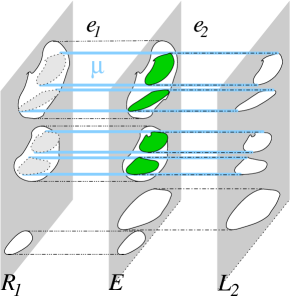
Figure 4: The (partial) composition of two rules is mediated by the dependency graph $E$ and the two matching morphisms $e_{1}$ and $e_{2}$. Since these are subgraph isomorphisms in our case, $E$ is simply the union $e_{1}(R_{1})\cup e_{2}(L_{2})$. The (partial) match $e_{1}(R_{1})\cap e_{2}(L_{2})$ can be understood as a matching $\mu$ between $R_{1}$ and $L_{2}$, i.e., as a 1-1 relation of the matching nodes and edges. Whenever an edge is matched, then so are its incident vertices.

3 Constructing Rule Compositions

Given two rules, $p_{1}$ and $p_{2}$, it is not only interesting to know if a partial composition is defined, but also to create the set of all possible compositions

$$\left\{p_{2}\circ_{\mu_{1}}p_{1},p_{2}\circ_{\mu_{2}}p_{1},\dots,p_{2}\circ_{\mu_{k}}p_{1}\right\}$$

explicitly. This set in particular contains also all full compositions. The following describes an algorithm for enumerating all partial compositions.

3.1 Enumerating the Matchings $\mu$

The key to finding all compositions is the enumeration of all matchings $\mu$ that respect out restrictions on overlaps between connected components. We thus start from the sets $\left\{R_{1}^{1},R_{1}^{2},\dots,R_{1}^{\#R_{1}}\right\}$ and $\left\{L_{2}^{1},L_{2}^{2},\dots,L_{2}^{\#L_{2}}\right\}$ of connected components of $R_{1}$ and $L_{2}$, resp. In the first set we find all subgraph matches $L_{2}^{i}\subseteq R_{1}^{j}$ (represented as the corresponding matchings $\mu_{ij}$) and arrange the result in a matrix of lists of subgraph matches, Fig. 5a.

$R_{1}^{1}$ $R_{1}^{2}$ $R_{1}^{3}$ $L_{2}^{1}$ 1 2 $L_{2}^{2}$ 1 1 (a) Match matrix

$R_{1}^{1}$ $R_{1}^{2}$ $R_{1}^{3}$ $R_{1}^{\emptyset}$ $L_{2}^{1}$ 1 2 1 $L_{2}^{2}$ 1 1 1 (b) Extended match matrix

Figure 5: Example of a match matrix and the same matrix with its virtual extension. The top row specifies 1 possibility for $L_{2}^{1}\subseteq R_{1}^{1}$ and 2 for $L_{2}^{1}\subseteq R_{1}^{3}$. The extended matrix further specifies that $L_{2}^{1}$ can be unmatched. The bottom rows can be interpreted similarly. We display the number of matchings instead of a representation of the matchings themselves.

The matching matrix is extended by a virtual column to account for the possibility that $L_{2}^{i}$ is not matched with any component of $R_{1}$. Every partial (and full) composition is now defined by a selection of one submatch from each row of the matrix, see Supplemental Material for an example. The converse is not true, however: Not every selection of matches correspond to a partial composition. In particular, we exclude the case that only entries from the virtual column are selected. In addition, the sub-matches must be disjoint to ensure that the combined match is injective. The latter conditions needs to be checked only when more than one submatch is selected from the same column.

3.2 Composing the Rules

The construction of the composition $p_{2}\circ_{\mu}p_{1}$ of two rules $p_{1}$ and $p_{2}$ does not explicitly depend on the component structure of $R_{2}$ and $L_{1}$ because it is uniquely defined by the matching $\mu$ and the bijections of the nodes of $L_{i}$, $K_{i}$, and $R_{i}$ for each of the two rules. We obtain $L$ by extending $L_{1}$ with unmatched components of $L_{2}$ and $R$ by extending $R_{2}$ by the unmatched components of $R_{1}$. The corresponding extension of $\mu$ to a bijection $\hat{\mu}$ of the vertex sets of $L$ and $R$ is uniquely defined. The context $K$ of the composite rule simply consists the common vertex set of $L$ and $R$ and all edges $(x,y)$ of $L$ for which $(\hat{\mu}(x),\hat{\mu}(y))$ is an edge in $R$. We note in passing that $\hat{\mu}$ defines the atom mapping of the composite transformation. The explicit construction of $(R,K,L)$ is summarized as Algorithm 3.1.

Input: $p_{1}=(L_{1},K_{1},R_{1})$

Input: $p_{2}=(L_{2},K_{2},R_{2})$

Input: $\mu$, a partial matching between $L_{2}$ and $R_{1}$

Output: $p=(L,K,R)$

1 $p\leftarrow$ empty rule

2 Copy vertices of $p_{1}$ to $p$

3 foreach vertex $v\in p_{2}$ do

4       if $v$ is not mapped by $\mu$ then

5             Copy $v$ to $p$

6      else

7             Change membership in $L$, $K$ and $R$ for vertex $\mu(v)$

8Copy edges of $p_{1}$ to $p$

9 foreach Edge $e\in p_{2}$ do

10       if $e$ is not mapped by $\mu$ then

11             Copy $e$ to $p$

12      else

13             Change membership in $L$, $K$ and $R$ for edge $\mu(e)$

14Delete edges and vertices created by $p_{1}$, but deleted by $p_{2}$

15 if matching condition not satisfied then abort

16

return $p$

Algorithm 3.1 Composing $p_{1}$ and $p_{2}$ to $p$, by a given partial mapping

The implementation of the algorithm naturally depends heavily on the representation of transformation rules, which in our implementation is the representation from the Graph Grammar Library (GGL) [6]. The representation is a single graph, with attached vertex and edge properties defining membership of $L$, $K$ and $R$, as well as the needed labels.

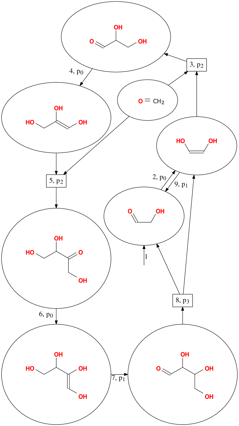
Figure 6: Above: Chemical reaction network for the Formose reaction; hyperedges are labeled with $(i,\mathsf{p_{j}})$ where $i$ is the $i$-th reaction $\rho_{i}$ in the rule composition. $\mathsf{p_{j}},0\leq j\leq 3$, refers to a specific rule from the Formose reaction; Right: Resulting composed rule after the composition of the first $i$ rules along the Formose cycle, context shown in black.

Not all matchings define valid rule composition. For instance, consider an edge $(u,v)$ that is present in $R_{1}$ and $R_{2}$ but not in $L_{2}$ and both $u$ and $v$ are in $L_{2}$. This would amount to creating the edge by means of rule $p_{2}$ which was already introduced by $p_{1}$. Since we do not allow parallel edges and thus regard such inconsistencies as undefined cases and reject the matching. Note that a parallel edge does not correspond to a “double bond” (which essentially is only an edge with a specific type).

3.3 Graph Binding

The composition of transformation rules, and thereby chemical reactions, makes it possible to create abstract meta-rules in a way that is similar to the combination of multiple functions into more abstract functions in functional programming. A related concept from (functional) programming that seems useful in the context of graph grammars is partial function application. Consider, for example, the binding of the number $2$ to the exponentiation operator, yielding either the function $f(x)=2^{x}$ or $f(x)=x^{2}$. In the framework of rule composition, we define graph binding as a special case.

Let $G$ be a graph and $p_{2}=(L_{2},K_{2},R_{2})$ be a transformation rule. The binding of $G$ to $p_{2}$ results in the transformation rule $p=(L,K,R)$ which implements the partial application of $p_{2}$ on $G$. This is accomplished simply by regarding $G$ as a rule $p_{1}=(\emptyset,\emptyset,G)$, and using partial composition; $p=p_{2}\circ p_{1}$. Note that if $p_{2}\circ p_{1}$ is a full composition, then $p$ can be regarded as a graph $H$ and $G\xRightarrow{p_{2}}H$ holds.

Graph binding allows a simplified representation of reactions. For instance, we can use this formal construction to omit uninteresting ubiquitously present molecules such as water by binding the graph of the water molecule to the transformation rule of a reaction that requires water. Similarly, graph unbinding can be defined as a transformation rule that destroys graphs. In a chemical application it can be used to avoid the explicit representation of uninteresting ubiquitous molecules such as the solvent.

3.4 Ordering Rules

A wide variety of methods, including flux balance analysis, can be used to identify pathways or other subsets of reactions that are of interest. Adjacency of reactions in the original networks as well as their directionality can be used efficiently to prune the possible orders of rule compositions. The fact that multiple reactions are instantiations of the same transformation rule, as in the example discussed in detail in the next section, further reduces the search spaces.

4 Results and Discussion

We illustrate the use of transformation rule composition by deriving of meta-rules from the graph grammar consisting of the four rules necessary to represent the complete Formose reaction, see Fig. 3. The overall reaction pattern of the Formose cycle is $2g_{0}+g_{1}\rightarrow 2g_{1}$ with $g_{0}$ being formaldehyde and $g_{1}$ being glycolaldehyde. It amounts to the linear combination $\sum_{i=1}^{9}\rho_{i}$ of the eight reactions and the influx $\rho_{1}$ of $g_{0}$ listed in Fig. 3. It is important to notice that several of these reactions are instantiations of the same, well-known chemical transformations. We have forward keto-enol tautomerism ($\mathsf{p_{0}}$: $\rho_{2}$, $\rho_{4}$, $\rho_{6}$), backward keto-enol tautomerism ($\mathsf{p_{1}}$: $\rho_{7}$, $\rho_{9}$), forward aldol addition ($\mathsf{p_{2}}$: $\rho_{3}$, $\rho_{5}$), and backward aldol addition ($\mathsf{p_{3}}$: $\rho_{8}$). The composite rule models the complete autocatalytic cycle shown in Fig. 6 as a single meta-rule.

Throughout this section we will not explicitly distinguish between partial composition and full composition, and we interpret the composition operator $\circ$ as right-associative to simplify the notation. Thus $p_{i}\circ p_{j}\circ p_{k}$ means $p_{i}\circ(p_{j}\circ p_{k})$.

The rules are used in the autocatalytic cycle in the following order (starting with an keto-enol tautomerisation $\mathsf{p_{0}}$):

$$\mathsf{p_{0},p_{2},p_{0},p_{2},p_{0},p_{1},p_{3},p_{1}}$$

As it is not possible to compose this sequence of rules directly, we start by binding glycolaldehyde $g_{1}$ to reaction $p_{0}$, as the before-mentioned keto-enol tautomerisation is applied to molecule $g_{1}$. The resulting rule is denoted as $\mathsf{g_{1}}$. The hyperedges in the chemical reaction network depicted in Fig. 6 are numbered according to the sequence that reflects in which order the Formose reaction takes place and consequently the order in which the rule composition subsequently is done. The first composition refers to the binding operation. This binding of glycolaldehyde results in a graph grammar rule, which is depicted in row 1 in the table depicted in Fig. 6, i.e., the rule ($\emptyset$, $\emptyset$, $g_{1}$) (see “Graph Binding”). The numbers at the hyperedges ($2,3,\ldots 9$) refer to the second, third, $\ldots$, ninth reaction in the sequence of reactions given above. The graph grammar rule $\mathsf{p_{i}},0\leq i\leq 3$, used for the corresponding hyper-edge is given next to the sequence number. The rules inferred by a subsequent rule composition are given in rows $2$ to $9$ of the table.

The application of the final rule results in the composed meta-rule $\mathsf{p_{1}}\circ\mathsf{p_{3}}\circ\ldots\circ\mathsf{p_{0}}\circ\mathsf{g_{1}}$. This rule precisely covers the reaction pattern of the Formose reaction, namely how two formaldehyde molecules and one (bound) glycolaldehyde are transformed to two glycolaldehyde molecules. However note, that the rule is general enough such that any pair of molecules with aldehyde groups can be used, i.e., the inferred reaction pattern refers to a class of overall reactions and the product does not necessarily need to be glycolaldehyde.

The practical computation of these compositions takes less than a second in the current implementation. Even for substantially more general composition sequences the running time remains manageable. For instance, it takes less than $1$ minute to compute all composition sequences with a length $k\leq 10$ of the form $p_{i_{1}}\circ p_{i_{2}}\circ\dots\circ p_{i_{k}}\circ g_{q}$ with $i_{j}\in\{0,1,2,3\}$, based on the binding of one of the influx molecules $g_{0}$ or $g_{1}$. This results in 1875 different inferred composite rules.

Polymerization can also be viewed as a pathway in a chemical reaction network, albeit one of potentially infinite size. The same methods applied to the automatic inference of the overall reaction pattern of the Formose cycle can be directly applied to detecting composition rules for polymerization reactions. Importantly, even if a chemical reaction network is not given, the approaches presented in this paper can be used to automatically find sequences of reactions that will lead to polymerization. This can be realized by a straight-forward post-processing step: all that needs to be done is to check whether an inferred composite rule exhibits a replicated functional unit. Such polymerization meta-rules also enable the analysis of chemical systems with highly complex carbon skeletons such as the natural compound classes of the terpenes or the polyketides.

5 Conclusions

Graph grammars provide a convenient framework for modeling chemistries on different levels of abstraction. A chemically valid approach is to see any chemical reaction as a bi-molecular reaction. This requires graph grammar rules that cover changes of molecules in an rather explicit and detailed way. Understanding chemical reaction patterns usually requires spanning the chemical reaction networks based on such rules. Obviously, this approach suffers the inherent potential of an immense combinatorial explosion. In this paper we introduced the automatic inference of such higher-level chemical reaction pattern based on a formal approach for graph grammar rule combination. We analyzed the autocatalytic cycle of the Formose reaction and inferred its overall reaction pattern as a rule composition of nine rules. Rule composition is also naturally applicable to inferring patterns of polymerization reactions. Future work will include e.g. the analysis of terpene-based and hydrogen cyanide-based polymerization chemistry.

Acknowledgments

This work was supported in part by the Volkswagen Stiftung proj. no. I/82719, and the COST-Action CM0703 “Systems Chemistry” and by the Danish Council for Independent Research, Natural Sciences.

Supplemental Material:
Example of Enumeration of Compositions

In this Appendix we show the complete result of the composition of two (artificial) rules, $p_{1}$ and $p_{2}$, including the selection of submatches from the match matrix. The two rules are depicted in Fig. 7 with the extended match matrix of the composition $p_{2}\circ p_{1}$, that corresponds to the example of an extended match matrix as given in the paper. The rules in this section are all depicted with vertices that have an additional index. The numbering of the components is in increasing order wrt. to these indices, e.g., $L_{2}^{1}$ denotes the component connecting nodes $A,0$ and $B,1$ and $L_{2}^{2}$ denotes the component connecting nodes $B,2$ and $C,3$.

(a) $p_{1}$

(b) $p_{2}$

	$R_{1}^{1}$	$R_{1}^{2}$	$R_{1}^{3}$	$R_{1}^{\emptyset}$
$L_{2}^{1}$	1		2	1
$L_{2}^{2}$		1	1	1

(c) Extended match matrix

Figure 7: The two rules $p_{1}$ and $p_{2}$, and the extended match matrix of the composition $p_{2}\circ p_{1}$. The components of both $R_{1}$ and $L_{2}$ are numbered in the same order as the vertex indices.

In the following we will enumerate all valid selections of submatches based on the extended match matrix and give the corresponding resulting rule composition. The chosen matches are depicted as • in the extended match matrix. If several matches can be found (in our example this is true for the component $L_{2}^{1}$, that can be matched twice in $R_{1}^{3}$), the • has an index.

Composition 1

	$R_{1}^{1}$	$R_{1}^{2}$	$R_{1}^{3}$	$R_{1}^{\emptyset}$
$L_{2}^{1}$	•
$L_{2}^{2}$		•

Result of composition 1

Composition 2

	$R_{1}^{1}$	$R_{1}^{2}$	$R_{1}^{3}$	$R_{1}^{\emptyset}$
$L_{2}^{1}$			•1
$L_{2}^{2}$		•

Result of composition 2

Composition 3

	$R_{1}^{1}$	$R_{1}^{2}$	$R_{1}^{3}$	$R_{1}^{\emptyset}$
$L_{2}^{1}$			•2
$L_{2}^{2}$		•

Result of composition 3

Composition 4

	$R_{1}^{1}$	$R_{1}^{2}$	$R_{1}^{3}$	$R_{1}^{\emptyset}$
$L_{2}^{1}$				•
$L_{2}^{2}$		•

Result of composition 4

Composition 5

	$R_{1}^{1}$	$R_{1}^{2}$	$R_{1}^{3}$	$R_{1}^{\emptyset}$
$L_{2}^{1}$	•
$L_{2}^{2}$			•

Result of composition 5

Composition 6

	$R_{1}^{1}$	$R_{1}^{2}$	$R_{1}^{3}$	$R_{1}^{\emptyset}$
$L_{2}^{1}$			•1
$L_{2}^{2}$			•

Result of composition 6

Invalid Selection

	$R_{1}^{1}$	$R_{1}^{2}$	$R_{1}^{3}$	$R_{1}^{\emptyset}$
$L_{2}^{1}$			•2
$L_{2}^{2}$			•

This selection of submatches is invalid, as they are not disjoint (node $B,9$ would be matched twice).

Composition 7

	$R_{1}^{1}$	$R_{1}^{2}$	$R_{1}^{3}$	$R_{1}^{\emptyset}$
$L_{2}^{1}$				•
$L_{2}^{2}$			•

Result of composition 7

Composition 8

	$R_{1}^{1}$	$R_{1}^{2}$	$R_{1}^{3}$	$R_{1}^{\emptyset}$
$L_{2}^{1}$	•
$L_{2}^{2}$				•

Result of composition 8

Composition 9

	$R_{1}^{1}$	$R_{1}^{2}$	$R_{1}^{3}$	$R_{1}^{\emptyset}$
$L_{2}^{1}$			•1
$L_{2}^{2}$				•

Result of composition 9

Composition 10

	$R_{1}^{1}$	$R_{1}^{2}$	$R_{1}^{3}$	$R_{1}^{\emptyset}$
$L_{2}^{1}$			•2
$L_{2}^{2}$				•

Result of composition 10

References

- Aittokallio and Schwikowski [2006] Tero Aittokallio and Benno Schwikowski. Graph-based methods for analysing networks in cell biology. Brief Bioinform, 7(3):243–255, 2006. doi: 10.1093/bib/bbl022.
- Benkö et al. [2003] Gil Benkö, Christoph Flamm, and Peter F Stadler. A graph-based toy model of chemistry. J Chem Inf Comput Sci, 43(4):1085–1093, 2003. doi: 10.1021/ci0200570.
- Dittrich et al. [2001] P. Dittrich, J. Ziegler, and W. Banzhaf. Artificial chemistries - a review. Artificial life, 7(3):225–275, 2001.
- Ehrig et al. [1991] H. Ehrig, A. Habel, H.-J. Kreowski, and F. Parisi-Presicce. Parallelism and concurrency in high-level replacement systems. Math. Struct. Comp. Science, 1:361–404, 1991.
- Ehrig et al. [2006] Hartmut Ehrig, Karsten Ehrig, Ulrike Prange, and Gabriele Taenthzer. Fundamentals of Algebraic Graph Transformation. Springer-Verlag, Berlin, D, 2006.
- Flamm et al. [2010] C. Flamm, A. Ullrich, H. Ekker, M. Mann, D. Hogerl, M. Rohrschneider, S. Sauer, G. Scheuermann, K. Klemm, I. Hofacker, and P. F. Stadler. Evolution of metabolic networks: A computational frame-work. Journal of Systems Chemistry, 1(4), 2010. ISSN 1759-2208. doi: 10.1186/1759-2208-1-4.
- Golas [2010] Ulrike Golas. Analysis and Correctness of Algebraic Graph and Model Transformations. Vieweg+Teubner, Wiesbaden, D, 2010.
- Klamt et al. [2009] Steffen Klamt, Utz-Uwe Haus, and Fabian Theis. Hypergraphs and cellular networks. PLoS Comput Biol, 5(5):e1000385, 2009. doi: 10.1371/journal.pcbi.1000385.
- Larhlimi and Bockmayr [2009] A. Larhlimi and A. Bockmayr. A new constraint-based description of the steady-state flux cone of metabolic networks. Discr. Appl. Math., 157:2257–2266, 2009.
- Orth et al. [2010] J. D. Orth, I. Thiele, and B. Ø. Palsson. What is flux balance analysis? Nature Biotech., 28:245–248, 2010.
- Price et al. [2003] N. D. Price, J. L. Reed, J. A. Papin, S. J. Wiback, and B. Ø. Palsson. Network-based analysis of metabolic regulation in the human red blood cell. J. Theor. Biol., 225:185–194, 2003.
- Schuster et al. [2000] S. Schuster, D. A. Fell, and T. Dandekar. A general definition of metabolic pathways useful for systematic organization and analysis of complex metabolic networks. Nature Biotech., 18:326–332, 2000.