The consequences of $SU(3)$ colorsingletness, Polyakov Loop and $Z(3)$ symmetry on a quark-gluon gas

Abstract

Based on quantum statistical mechanics we show that the $SU(3)$ color singlet ensemble of a quark-gluon gas exhibits a $Z(3)$ symmetry through the normaized character in fundamental representation and also becomes equivalent, within a stationary point approximation, to the ensemble given by Polyakov Loop. Also Polyakov Loop gauge potential is obtained by considering spatial gluons along with the invariant Haar measure at each space point. The probability of the normalized character in $SU(3)$ vis-a-vis Polyakov Loop is found to be maximum at a particular value exhibiting a strong color correlation. This clearly indicates a transition from a color correlated to uncorrelated phase or vise-versa. When quarks are included to the gauge fields, a metastable state appears in the temperature range $145\leq T({\rm{MeV}})\leq 170$ due to the explicit $Z(3)$ symmetry breaking in the quark-gluon system. Beyond $T\geq 170$ MeV the metastable state disappears and stable domains appear. At low temperature a dynamical recombination of ionized $Z(3)$ color charges to a color singlet $Z(3)$ confined phase is evident along with a confining background that originates due to circulation of two virtual spatial gluons but with conjugate $Z(3)$ phases in a closed loop. We also discuss other possible consequences of the center domains in the color deconfined phase at high temperature.

1 Introduction:

A statistical thermodynamical description of a quantum gas, is often useful for various physical systems, e.g., electrons in metal, blackbody photons in a heated cavity, phonons at low temperature, neutron matter in neutron stars, etc. In most cases the mutual interactions among the constituents is neglected, although they interact in order to come to a thermal equilibrium. One can imagine a situation by first allowing them to come to a thermal equilibrium and then slowly turning off the interactions [1]. In a same perspective, we consider a quantum gas of non-interacting quarks ($q$), antiquarks ($\bar{q}$) and gluons ($g$) with the underlying symmetry of $SU(3)$ color gauge theory at a given temperature. Such a simple quantum statistical description exhibits very interesting features of a quark-gluon system.

2 Quantum statistical mechanics and color singlet ensemble:

In thermal equilibrium the statistical behaviour of a quantum gas is studied through a density matrix in an appropriate ensemble as

$${\rho(\beta)}={\rm{exp}}(-\beta{\hat{H}})\ \ ,$$ (1)

where $\beta=1/T$ is the inverse of temperature and ${\hat{H}}$ is the Hamiltonian of a physical system. The corresponding partition function for a quantum gas having a finite volume can be written as

$${\cal Z}={\rm{Tr}}\left(e^{-\beta{\hat{H}}}\right)=\sum_{n}\left\langle n\left|e^{-\beta{\hat{H}}}\right|n\right\rangle\ \ ,$$ (2)

where $|n\rangle$ is a many-particle state in the full Hilbert space ${\cal H}$. Now, the full Hilbert space contains states which should not contribute to a desired configuration of the system. One can restrict those states from contributing to the partition function by defining a reduced ensemble for a desired configuration as

$${\cal Z}={\rm{Tr}}\left({\hat{\cal P}}e^{-\beta{\hat{H}}}\right)=\sum_{n}\left\langle n\left|{\hat{\cal P}}e^{-\beta{\hat{H}}}\right|n\right\rangle\ \ .$$ (3)

Now, let ${\cal G}$ be a symmetry group with unitary representation ${\hat{U}}(g)$ in a Hilbert space ${\cal H}$. The projection operator [2, 3, 4, 5, 6] ${\hat{\cal P}}$ for a desired configuration is defined as ${\hat{\cal P}}_{j}=d_{j}\int_{\cal G}{\rm d}\mu(g)\chi^{\star}_{j}(g){\hat{U}}(g)$ , where $d_{j}$ and $\chi_{j}$ are, respectively, the dimension and the character of the irreducible representation $j$ of ${\cal G}$ and ${\rm d}\mu(g)$ is the invariant Haar measure. The symmetry group associated with the color singlet configuration is $SU(N_{c})$ and $d_{j}=1$ and $\chi_{j}=1$. Now the color singlet partition function for the system becomes,

$${\cal Z}_{S}=\int_{SU(N_{c})}{\rm d}\mu(g){\rm{Tr}}\left({\hat{U}}(g){\rm{exp}}(-\beta{\hat{H}})\right)\ \ .$$ (4)

The invariant Haar measure [2, 3] is expressed in terms of the distribution of eigenvalues of $SU(N_{c})$ as

$$\int{\rm d}\mu(g)\!\!=\!\!\frac{1}{N_{c}!}\!\left(\prod^{N_{c}}_{i=1}\!\int\limits_{-\pi}^{\pi}\frac{{\rm d}\theta_{l}}{2\pi}\right)\delta(\sum_{i}\theta_{i})\!\!\prod_{i>j}\left|e^{i\theta_{i}}-e^{i\theta_{j}}\right|^{2},$$ (5)

where the square of the product of the differences of the eigenvalues is known as the Vandermonde (VdM) determinant. The class parameter $\theta_{l}$ obeys $\sum^{N_{c}}_{l=1}\theta_{l}=0\ ({\rm{mod}}2\pi)$ ensuring the requirement of unit determinant in $SU(N_{c})$. This also restricts that the $SU(3)$ has only two parameter abelian subgroups associated with two diagonal generators, which would completely characterize the ${\hat{U}}(g)$.

Now, the Hilbert space ${\cal H}$ of a composite system has a structure of a tensor product of the individual Fock spaces as ${\cal H}={\cal H}_{q}\otimes{\cal H}_{\bar{q}}\otimes{\cal H}_{g}$. The partition function in (4) decomposes [3, 4, 5, 6] in respective Fock spaces as

$${\cal Z}_{S} = \int_{SU(N_{c})}{\rm d}\mu(g)\,{\rm{Tr}}\left({\hat{U}}_{q}e^{-\beta{\hat{H}}_{q}}\right){\rm{Tr}}\left({\hat{U}}_{\bar{q}}e^{-\beta{\hat{H}}_{\bar{q}}}\right)\,{\rm{Tr}}\left({\hat{U}}_{g}e^{-\beta{\hat{H}}_{g}}\right),$$ (6)

where the various $U_{i}(g)$ act as link variables that link, respectively, the quarks, antiquarks and spatial gluons in a given state of the physical system. In each Fock space there exists a basis that diagonalizes both operators as long as ${\hat{H}}_{i}$ and ${\hat{U}}_{i}$ commute. Performing the traces in (6) using the standard procedure [1, 3, 5], the partition function in Hilbert space becomes

$${\cal Z}_{S}\!\! = \!\!\!\int_{SU(N_{c})}\!\!\!\!\!\!\!\!\!{\rm d}\mu(g)\ \ e^{\Theta_{q}+\Theta_{\bar{q}}+\Theta_{g}}=\int_{SU(N_{c})}{}\!\!\!{\rm d}\mu(g)\ \ e^{\Theta_{p}}\ \ ;$$ (7)

$$\Theta_{p} = \Theta_{q}+\Theta_{\bar{q}}+\Theta_{g}$$ (8)

$$= 2N_{f}\sum_{\alpha}{\rm{tr}_{c}}\ln\left(1+R_{q}e^{-\beta(\epsilon_{q}^{\alpha}-\mu_{q})}\right)+2N_{f}\sum_{\alpha}{\rm{tr}_{c}}\ln\left(1+R_{\bar{q}}e^{-\beta(\epsilon_{q}^{\alpha}+\mu_{q})}\right)$$

$$-2\sum_{\alpha}{\rm{tr}_{c}}\ln\left(1-R_{g}e^{-\beta\epsilon_{g}^{\alpha}}\right),$$

where $\epsilon_{i}^{\alpha}=\sqrt{(p^{\alpha}_{i})^{2}+m^{2}_{i}}$. Also the quark flavor ($N_{f}$), their spin and the chemical potential $\mu$, and the polarization of gluons are introduced. The finite dimensional diagonal matrix $R_{q({\bar{q}})}$ in the basis of the color space represents the image [2, 3] of the group element in the irreducible representation of $SU(N_{c})$ as

$${R}_{q} = \mbox{diag}\left(e^{i\theta_{1}}\,,e^{i\theta_{2}}\,,e^{i\theta_{3}}\right)\,;\hskip 21.68121pt{R}_{\bar{q}}=R^{\dagger}_{q},$$ (9)

with their respective characters

$$\chi_{f}=\mbox{tr}_{c}R_{q}=\sum_{i=1}^{N_{c}}e^{i\theta_{i}};\hskip 21.68121pt\chi_{f}^{\dagger}=\mbox{tr}_{c}R_{q}^{\dagger}=\sum_{i=1}^{N_{c}}e^{-i\theta_{i}}.\$$ (10)

Similarly, the character in adjoint representation is obtained as

$$\chi_{\mbox{adj}} = \chi_{f}\chi_{f}^{\dagger}-1=\mbox{tr}_{c}R_{g}=\mbox{tr}_{c}\Big{[}\mbox{diag}\big{(}1,1,e^{i(\theta_{1}-\theta_{2})},e^{-i(\theta_{1}-\theta_{2})},$$ (11)

$$e^{i(2\theta_{1}+\theta_{2})},e^{-i(2\theta_{1}+\theta_{2})},e^{i(\theta_{1}+2\theta_{2})},e^{-i(\theta_{1}+2\theta_{2})}\Big{)}\Big{]}$$

We also define normalized characters by the respective dimension of the fundamental and adjoint representations as

$$\Phi=\frac{1}{N_{c}}{\rm{tr}_{c}}R_{q}\,\,,\quad\quad\bar{\Phi}=\frac{1}{N_{c}}{\rm{tr}_{c}}R_{q}^{\dagger}\,\,,\quad\quad(N_{c}^{2}-1)\Phi_{A} = N_{c}^{2}\Phi{\bar{\Phi}}-1\,.$$ (12)

As we will see in the next sec. that the magnitude of the normalized character, $|\Phi|$, in fundamental representation is related to the thermal expectation value of the Polyakov Loop (PL).

The VdM term in (5) can now be written in terms of $\Phi$ and ${\bar{\Phi}}$ as

$$\prod_{i>j}^{3}\left|e^{i\theta_{i}}-e^{i\theta_{j}}\right|^{2} = 27[1-6\Phi{\bar{\Phi}}+4(\Phi^{3}+{\bar{\Phi}}^{3})-3(\Phi{\bar{\Phi}})^{2}]=27\ H(\Phi,{\bar{\Phi}})\,,$$ (13)

for $SU(3)$. Further, this is in general not possible for $N_{c}>3$ as there are more than two independent parameters. Now the Jacobian for variable transformation from $\{\theta_{1},\theta_{2}\}$ to $\{\Phi,{\bar{\Phi}}\}$ can be obtained as

$$J(\Phi,{\bar{\Phi}})={(1/9)}\sqrt{27H(\Phi,{\bar{\Phi}})}.$$ (14)

In the infinite volume $V$, one also needs to replace the discrete single particle sum by an integral as $\sum_{\alpha}\rightarrow(V/(2\pi)^{3}\int d^{3}p\ .$

After performing the color trace of the matter and gauge parts, and expressing in terms of the characters of the fundamental and its conjugate, Eq.(7) becomes

$${\cal Z}_{S} = \int_{SU(3)}\ d\Phi\ d{\bar{\Phi}}\ e^{\Theta_{q}+\Theta_{\bar{q}}+\Theta_{g}+\Theta_{H}};$$

$$\Theta = \Theta_{q}+\Theta_{\bar{q}}+\Theta_{g}+\Theta_{H}$$ (15)

$$= 2VN_{f}\int\frac{d^{3}p}{(2\pi)^{3}}\ln\Big{[}1+e^{-3\beta\epsilon_{q}^{+}}+N_{c}\left(\Phi+\bar{\Phi}e^{-\beta\epsilon_{q}^{+}}\right)e^{-\beta\epsilon_{q}^{+}}\Big{]}$$

$$+2VN_{f}\int\frac{d^{3}p}{(2\pi)^{3}}\ln\left[1+e^{-3\beta\epsilon_{q}^{-}}+N_{c}\left({\bar{\Phi}}+{\Phi}e^{-\beta\epsilon_{q}^{-}}\right)e^{-\beta\epsilon_{q}^{-}}\right]$$

$$-2V\int\frac{d^{3}p}{(2\pi)^{3}}\ln\Big{(}1+\sum_{m=1}^{8}a_{m}\,e^{-m\beta\epsilon_{g}}\Big{)}+\frac{n}{2}\ln H.$$

with $\epsilon^{\pm}_{q}={\epsilon_{q}\mp\mu}$ and the coefficients $a_{m}$ are given by

$$a_{1} = a_{7}=1-N_{c}^{2}\bar{\Phi}\Phi\,,\quad a_{8}=1\,,$$

$$a_{2} = a_{6}=1-3N_{c}^{2}\bar{\Phi}\Phi{}+N_{c}^{3}\left(\bar{\Phi}^{3}+\Phi^{3}\right)\,,$$

$$a_{4} = 2\left[-1+N_{c}^{2}\bar{\Phi}\Phi-N_{c}^{3}\left(\bar{\Phi}^{3}+\Phi^{3}\right){}+N_{c}^{4}\left(\bar{\Phi}\Phi\right)^{2}\right]\,,$$

$$a_{3} = a_{5}=-2+3N_{c}^{2}\bar{\Phi}\Phi{}-N_{c}^{4}\left(\bar{\Phi}\Phi\right)^{2}\,.$$ (16)

We note here that the square of the VdM determinant in (5) enters at each point in space in the action. So, in the partition function the logarithm of the product of the VdM term should be proportional to $n$ as $\Theta_{H}=n\ln\sqrt{H}$, assuming $n$ is the number of points in the space. Also a constant normalization factor is dropped as it is subleading.

Now performing the integrations using the method of stationary points, one can write

$${\cal Z}_{S}^{0}\!\! = \!\!\left.e^{\Theta_{q}+\Theta_{\bar{q}}+\Theta_{g}+\Theta_{H}}\right|_{\Phi\rightarrow\Phi_{0}\atop{\bar{\Phi}}\rightarrow{\bar{\Phi}_{0}}},$$ (17)

where the stationary values of $\Phi_{0}$ and ${\bar{\Phi}_{0}}$ can be obtained from the extremum conditions as

$$\frac{\partial\Theta}{\partial\Phi} = 0\,;\,\,\,\,\,\,\frac{\partial\Theta}{\partial{\bar{\Phi}}}=0\,.$$ (18)

The color singlet thermodynamic potential density at the stationary points in infinite volume limit becomes

$${\Omega}_{S}^{0} = -\frac{T}{V}\ln{\cal Z}_{S}^{0}=-\frac{T}{V}\left[\Theta_{q}+\Theta_{\bar{q}}+\Theta_{g}+\Theta_{\mbox{H}}\right]_{\Phi\rightarrow\Phi_{0}\atop{\bar{\Phi}}\rightarrow{\bar{\Phi}_{0}}}$$ (19)

$$= \Big{[}\Omega_{q}+\Omega_{\bar{q}}+\Omega_{g}-\kappa T\ln H\Big{]}_{\Phi\rightarrow\Phi_{0}\atop{\bar{\Phi}}\rightarrow{\bar{\Phi}_{0}}}={\Omega}^{\mbox{PL}}(\Phi_{0},{\bar{\Phi}_{0}}).$$

where $`$PL’ stands for Polyakov Loop [7, 8, 9]. This exhibits that the $SU(3)$ color singlet ensemble of a quark-gluon gas is equivalent to that of the Polyakov Loop. We derived the ensemble of the Polyakov Loop model phenomenologically by imposing $SU(N_{c})$ color singlet restriction on a quark-gluon gas. Also the Polyakov Loop gauge potential is obtained here as $\Omega_{g}-\kappa T\ln H$, by considering the spatial gluons in the ensemble. In some other context the gluons as quasiparticles in Polyakov Loop model was also studied [10, 11] but in most phenomenological studies the form of the gauge potential has usually been used [9, 12] by fitting pure gauge lattice data.

We note here that the calculation begun with a discussion of color neutrality effects in the free quark-gluon gas [3, 4, 5, 6]. These works were concerned with global color neutrality and the effect of which becomes irrelevant for a free gas in the limit where volume goes to infinity. Here, the extension to local neutrality is considered using Haar measure at every spatial point to address the effect of confinement. Nevertheless, the well-known calculations of the effective potential for PL to one loop in perturbation theory [8] show that the local VdM contribution due to the Haar measure is canceled out when spatially longitudinal gluon fields ($A_{0}(t,{\mathbf{x}})$) are integrated over. This becomes a problem to use local Haar measure as the basis for a fundamental theory of confinement and presently it is not known yet how to use it. On the other hand, allowing PL field where $A_{0}(t,{\mathbf{x}})$ is constant (see in the next sec.) as ${\mathbf{x}}\rightarrow\infty$, the VdM term contributes to the partition function in (15) and thus in the potential in (19). We further note that the contribution from the VdM term survives infinite volume limit since the constant, $\kappa=n/2V$, is the ratio of two large numbers leading to a finite value which has to be determined from the lattice equation of state of pure $SU(3)$ gauge theory. This value is found as $\kappa\sim 0.0075$ GeV³ in the literature [12, 9]. Now, the potential in (19) has been considered [9] as a starting point for phenomenological models of quark-gluon thermodynamics and is also coupled to chiral model [13, 14] to study extensively the deconfinement and chiral dynamics together [9].

Now, in the next part we do not intend to study thermodynamics, instead we discuss below some of the phenomenological consequences of $SU(3)$ colorsingletness vis-a-vis Polyakov Loop that may lead to the formation of center domains [7, 15] in quark-gluon plasma produced in relativistic heavy-ion collisions.

3 Polyakov Loop and normalised character in $SU(3)$:

The Wilson line in $SU(N_{c})$ in the direction of Euclidean time $\tau$ is defined [7] as a path-ordering by

$$W(x)={\cal T}\exp[ig\int\limits_{0}^{\beta}A_{0}(x,\tau)\ d\tau]\,,$$ (20)

where $A_{0}=A_{0}^{a}\lambda_{a}$ is a temporal gauge field with Gell-Mann matrices $\lambda_{a}$ ($a=1,\cdots N_{c}^{2}-1$), $g$ is the strong coupling and $\cal T$ is the path-ordering in Euclidean time. The normalized trace of the Wilson line with respect to fundamental representation is known as Polyakov Loop,

$$L(x)=\frac{1}{N_{c}}{\mbox{tr}_{c}}W(x),$$ (21)

where the Polyakov Loop is a complex and transforms under the global $Z(N_{c})$ symmetry as a field with charge one as $L\rightarrow e^{{2\pi i}/{N_{c}}}L$. It also acts as an order parameter for pure gauge theory since the free energy of the heavy static quark, $F_{Q}$ is related to the thermal average of the Polyakov Loop as $|\langle L\rangle|=\exp[-\beta F_{Q}(T)]$.

Given the role of an order parameter for pure gauge [7], if $|\langle L\rangle|=0$ the $Z(N_{c}$) is unbroken and there is no ionization of $Z(N_{c})$ charge, which is the confined phase below a certain temperature. At high temperature the symmetry is spontaneously broken, $|\langle L\rangle|\neq 0$ corresponds to a deconfined phase of gluonic plasma and there are $N_{c}$ different equilibrium states distinguished by the phase $2\pi j/N_{c}$ with $j=0,\cdots(N_{c}-1)$.

In most of the phenomenological studies [9] $A_{0}$ is assumed to be a static temporal gauge field within Polyakov Loop gauge. $A_{0}$ would completely be characterized by two diagonal generators [11] as $A_{0}=A_{0}^{3}\lambda_{3}+A_{0}^{8}\lambda_{8}$. The thermal expectation of the gauge invariant Polyakov Loop in terms of the characters normalized by the dimension of the fundamental representation for $SU(3)$is given in (12) as

$$|\Phi|=\langle L\rangle\!=\!\left\langle\frac{1}{3}{\mbox{tr}_{c}}\left({\cal T}\exp\left[ig\!\!\int\limits_{0}^{\beta}\!A_{0}\ d\tau\right]\right)\right\rangle.$$ (22)

Now, assuming a gaussian approximation one can write [7, 12]

$$|\Phi| = \left|\frac{1}{3}{\rm{tr}_{c}}R_{q}\right|=\sqrt{\Phi{\bar{\Phi}}}=|\langle L\rangle|\approx\exp\left[-\frac{g^{2}}{2T^{2}}{\mbox{tr}}_{c}\langle A_{0}^{2}\rangle\right].$$ (23)

The dynamics of the magnitude of the normalized character, $|\Phi|$, in fundamental representation is governed by the thermal average of the square of the static temporal gauge field $A_{0}$. In the color confined phase $|\Phi|=0$ and the background temporal gauge field fluctuates with high amplitudes whereas in the color deconfined phase $|\Phi|=1$ and the fluctuations of the gauge field almost disappears. This background gauge field in the form of Polyakov Loop also interacts nonpertubatively with the quarks and gluons in the thermal medium as given in (19).

4 Normalised character, center symmetry and consequences

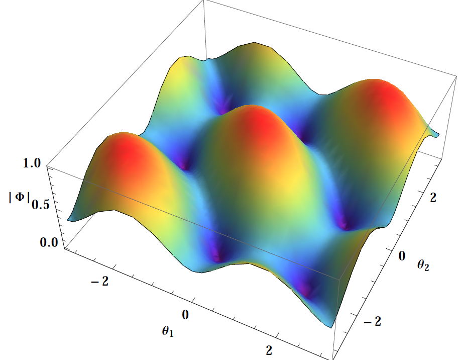
Figure 1: (color online) A $3$D-plot of $|\Phi(\theta_{1},\theta_{2})|$, i.e., the normalized character in the fundamental representation of $SU(3)$ as given in (12) within $-\pi\leq\theta_{1},\,\theta_{2}\leq\pi$.

In Fig. 1 a three dimensional view of the magnitude of the normalized character in fundamental representation of $SU(3)$, $|\Phi(\theta_{1},\theta_{2})|$, is shown within the domain $-\pi\leq\theta_{1},\theta_{2}\leq\pi$. It has three maxima for $(\theta_{1},\theta_{2})=(0,0),\,(2\pi/3,2\pi/3)\,(-2\pi/3,-2\pi/3)$. There are also three minima (and three mirror images exist if one interchanges $\theta_{1}\leftrightarrow\theta_{2}$) for $(\theta_{1},\theta_{2})=(0,2\pi/3),\,(0,-2\pi/3)\,{\mbox{and}}\,(2\pi/3,-2\pi/3)$. $|\Phi|$ has a three fold degeneracy connected by a rotation of $2\pi/3$ in both $\theta_{1}$ and $\theta_{2}$. A Monte Carlo simulation of complex $\Phi$ is also displayed in Fig. 2 in a Argand plane with $-\pi\leq(\theta_{1},\,\theta_{2})\leq\pi$. This shows a three pointed star in a circle of unit radius, in which each point can be rotated by a phase $2\pi/3$ except the origin. This clearly indicates that $\Phi$ in fundamental representation of $SU(3)$ has a center symmetry, $Z(3)$ with three rotational angles (viz., $0,\,2\pi/3,\,4\pi/3$ or $-2\pi/3$ ). This can also be understood from the invariant Haar measure expressed in terms of $\Phi$ in (13). Now, the three minima in Fig. 1 uniquely correspond to the center of the circle at $\Phi=0$ in Fig. 2, which is $Z(3)$ symmetric phase or confined phase at low $T$. On the other hand, the three maxima in Fig. 1 correspond to the three pointed tips in Fig. 2 representing the spontaneously broken phase or deconfined phase of $Z(3)$ at very high $T$. $\Phi$ can act as an order parameter for deconfinement phase transition. In Fig. 3 a three dimensional plot of $\Phi_{A}$ is also displayed that exhibits same features as Fig. 1 except minima appear in negative values, which could be understood from (12). This clearly suggests that the magnitude of the normalized character in the fundamental representation of $SU(3)$ exhibits the center symmetry, $Z(3)$.

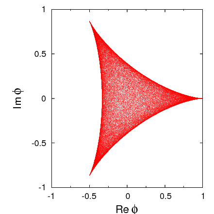
Figure 2: (color online) A Monte Carlo simulation of complex $\Phi(\theta_{1},\theta_{2})$ in Argand plane for which $\theta_{1}$ and $\theta_{2}$ are chosen randomly in the domain $-\pi\leq\theta\leq\pi$.

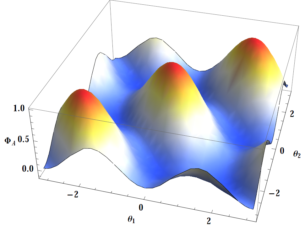
Figure 3: (color online) Same as Fig. 1 but for $\Phi_{A}(\theta_{1},\theta_{2})$.

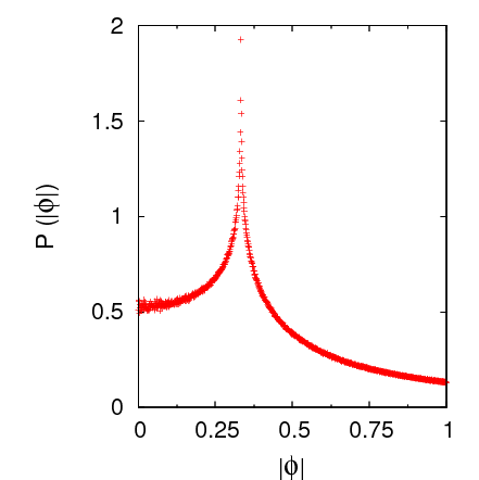
Figure 4: (color online) A Monte Carlo simulation, $P(\Phi)$, corresponds to the occurrence probability of $|\Phi(\theta_{1},\theta_{2})|$ in $SU(3)$ parameter space $(\theta_{1},\,\theta_{2})$. The values of $\theta_{1}$ and $\theta_{2}$ are chosen randomly within the domain $-\pi\leq\theta_{1},\,\theta_{2}\leq\pi$ and then the obtained value of $|\Phi|$ is mapped in a given $\Phi$ bin, which is then normalized by the area of the bin.

We also noticed some more interesting features of $\Phi$ in ($\theta_{1},\,\theta_{2}$)-plane. In Fig. 4 a Monte Carlo simulation of the occurrence probability, $P(|\Phi|)$, of $|\Phi(\theta_{1},\theta_{2})|$ is displayed in $SU(3)$ parameter space. This plot indicates that the maximum probability for $|\Phi|$ to occur when $|\Phi|=1/3$ indicating a phase transition from a color confining phase to a color deconfining phase, which has also been observed in Lattice QCD calculation [16]. This could be better viewed from Fig. 5 which is a contour plot corresponding to Fig. 1. As $T$ increases, $\Phi$ increases [9] from zero in the confined phase and reaches unity for ideal gas. In the domain $0<|\Phi|<1/3$, the color neutral states start decomposing but prefer to reside in $Z(3)$ minima and its mirror images minima. Color charges (partons) with thermal momentum in this domain cannot overcome the barriers provided by the large amplitude of the thermal fluctuations of the background gauge field in (23). This domain of $|\Phi|$ is shown by red dots ($|\Phi|\sim 0$) to purple triangles ($|\Phi|\sim 0.3$) in Fig. 5. As long as such states are inside the domain of $Z(3)$ minima, a strong color correlation exists among the color charges like a liquid [12], because the mean free path of the color charges is of the order of size of the domain in $Z(3)$ minima. In this $|\Phi|$ domain, the normalized character in adjoint representation varies as $-1/8\leq\Phi_{A}<0$ which is represented in Fig. 6.

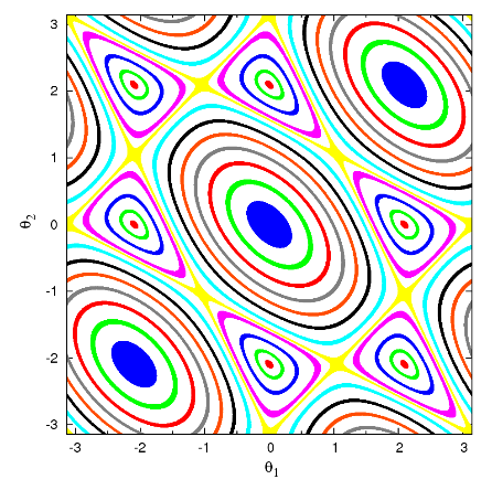
Figure 5: (color online) A 2D projection of $|\Phi|$ in $\theta_{1}$ and $\theta_{2}$ plane in which each color corresponds to a equivalued $|\Phi|$. The red dots to purple triangles correspond to $|\Phi|\sim 0,\,0.1,\,0.2,\,0.3$ whereas sea-blue lines to blue dots correspond to $|\Phi|\sim 0.4,\,0.5,\,0.6,\,0.7,\,0.8,\,0.9,1$. The equivalued mess connected by yellow triangles corresponds to $|\Phi|\sim 1/3$.

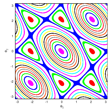
Figure 6: (color online) Same as Fig. 5 but for $\Phi_{A}$. The equivalued mess connected by blue triangles is for $\Phi_{A}=0$. From the blue mess to purple blobs, $\Phi_{A}$ increases by a step of $0.1$. The red dots are for $\Phi_{A}\sim-1/8$ whereas the green triangles $\Phi_{A}\sim-0.05$.

Now for $|\Phi|=1/3$, the $Z(3)$ minima disappear and get connected to each other in $Z(3)$ space, which is represented by the yellow mess in Fig. 5. This causes $P(|\Phi|)$ to be maximum in Fig. 4 exhibiting a long range color correlation and the thermal fluctuations of the background gauge field attain a critical value as the separating barriers of minima become flat and wider. Here $\Phi_{A}=0$ as is also represented by the blue mess in Fig. 6.

When $1/3<|\Phi|\leq 1$, the correlated $Z(3)$ domains start to get uncorrelated and the ionization of $Z(3)$ color charges begin which is evident from equivalued $|\Phi|$ lines in Fig. 5 starting from sea-blue ($|\Phi|\sim 0.4$) to green lines ($|\Phi|\sim 0.9$) at a step of $0.1$. When $|\Phi|\sim 1$ a complete ionization of $Z(3)$ charges take place and they reside at those maxima in Fig. 1 which are also represented by blue blobs in Fig. 5. This ionization can also be seen in Fig. 6 through purple equivalued $\Phi_{A}$ lines to purple blobs in the range $0.1\leq\Phi_{A}\leq 1$. So, in the color deconfined phase ($1/3<|\Phi|\leq 1$), there are formation of domains which are also separated by the nonperturbative interaction of the background gauge fields. These domains of ionized color charges can act as scattering centers in the deconfined phase lead to jet quenching. A hard jet after losing energy through gluon emission by the scattering with those ionized domain of color charges [12] in deconfined phase ($1/3<|\Phi|\leq 1$) can enter the confining phase ($0<|\Phi|\leq 1/3$) and hadronize by recombination [6, 17].

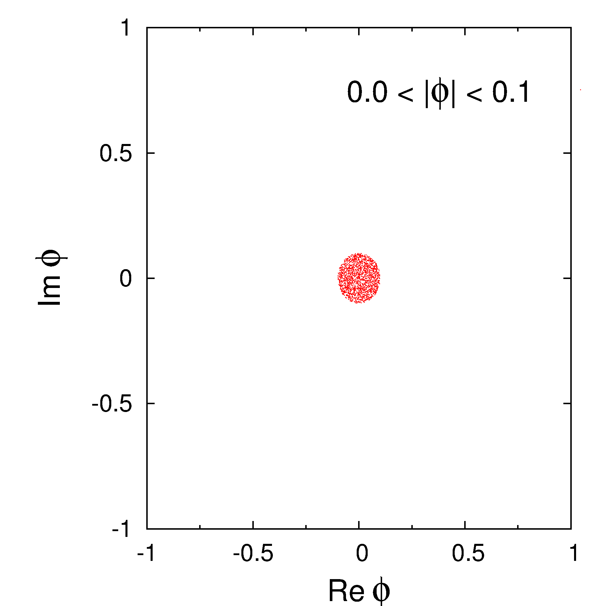
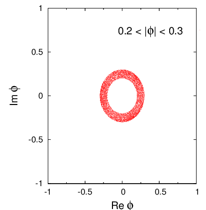
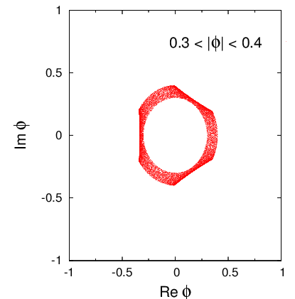
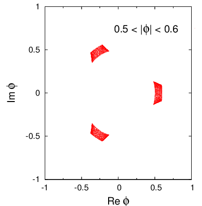
Figure 7: (color online) The projection of $\Phi$ in Argand plane for a fixed value, which are noted in the respective plots. This shows a strong color correlation in the range $0\leq\Phi\leq 1/3$ and ionization of color states in the range $1/3<\Phi\leq 1$.

All those features of center symmetry discussed above are also reflected in complex $\Phi$ plane in Fig. 7 indicating a snap shot of color localized and ionized domains of $Z(3)$. This clearly shows that there are center domains formation in the two distinct regions of $|\Phi|$, which are $0<|\Phi|\leq 1/3$ (confining domain) due to the center symmetry $Z(3)$, and $1/3<|\Phi|\leq 1$ (deconfining or ionization domain) due to spontaneously breaking of the center symmetry $Z(3)$. The broken center domains formed in deconfining phases ($\langle L\rangle\neq 0$ or $1/3<|\Phi|\leq 1$ ) will be separated by domain walls as they are distinguished by the phases $2\pi j/3$ with $j=0,1,2$. Nevertheless, the formation of the center domains, the path of ionization and the distribution of the color charges from confining phase to deconfining phase or vice-versa will also depend on the nature of the color singlet potential for pure gauge (where $Z(3)$ is spontaneously broken) and also that with matter field (where $Z(3)$ is explicitly broken), which we discuss below using (19).

4.1 Gauge Sector:

The color singlet gauge potential is obtained in (19) as

$$\Omega^{g}_{S} = \Omega_{g}-\kappa T\ln H$$ (24)

$$= 2T\int\frac{d^{3}p}{(2\pi)^{3}}\ln\left(1+\sum_{m=1}^{8}a_{m}\,e^{-m\beta\epsilon_{g}}\right)-\kappa T\ln H,$$

where the first term describes the interaction of the spatial gluons with the Polyakov Loop (background temporal gauge field $A_{0}$ in (23)) at finite $T$. The second term known as VdM term comes from invariant Haar measure. The $Z(3)$ domains are plentiful (viz., Eq.(2)) as the gluon dynamics are solely governed by the thermal fluctuation of the background gauge field $A_{0}$ in (23).

In Fig. 8 the color singlet gauge potential in a complex $\Phi$ plane is displayed for three temperatures. The left panel corresponds to 3-dimensional plots whereas right panel represents corresponding contour plots. As can be seen the gauge potential, below $T<270$ MeV, has only one global minimum whereas for $T\geq 270$ MeV, it shows three minima representing a spontaneously broken $Z(3)$ phase for pure gauge. The corresponding contour plots also display the same features. So, $T<270$ MeV is color confining phase, where $Z(3)$ is unbroken as there is no ionization of color charges. On the other hand $T\geq 270$ MeV there are ionization of color charges as the center symmetry is spontaneously broken and those charges reside at the three minima in the potential in Fig. 8 or three maxima in color space in Figs. 1 and 5 separated by distinct phases $2\pi j/3$ with $j=0,1,2$ and also by domain walls [12]. $T\sim(265-270)$ MeV, possibly indicates a phase transition for pure gauge and is in agreement with lattice result [18].

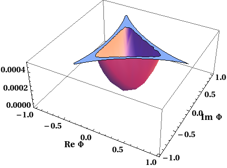
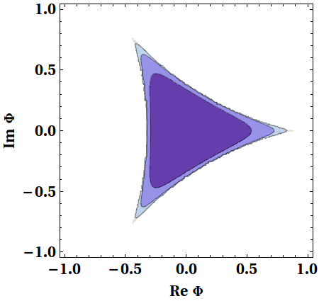
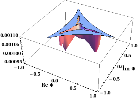
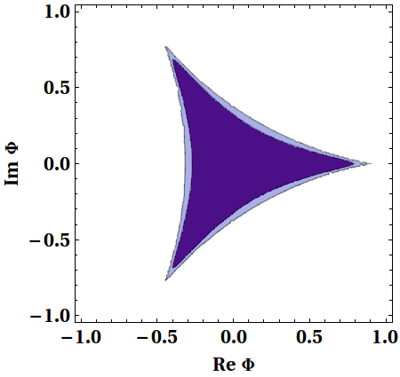
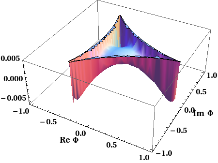
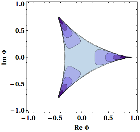
Figure 8: (color online) Left Panel: A 3D plot of $\Omega_{g}\,-\,\kappa T\ln\Theta_{H}$ in a complex $\Phi$ plane for $T=50,\,270,\,{\mbox{and}}\,350$ MeV and $\kappa=0.0075$ GeV³. Right Panel: Corresponding contour plots.

In asymptotically high temperatures ($T\gg T_{c}$), $\Phi,{\bar{\Phi}}\to 1$, $\langle{A}_{0}^{2}\rangle\to 0$, one recovers free gluon gas from $\Omega_{g}^{\rm{PL}}$ as

$$\Omega_{S}^{g;\;\Phi,{\bar{\Phi}}\rightarrow 1}\!\!\! = \!\!2(N_{c}^{2}-1)T\!\!\int\frac{d^{3}p}{(2\pi)^{3}}\ln\left(1-e^{-\beta\epsilon_{g}}\right),$$ (25)

where $N_{c}=3$. The VdM term due to the invariant Haar measure disappears and the spatial gluons are completely ionized.

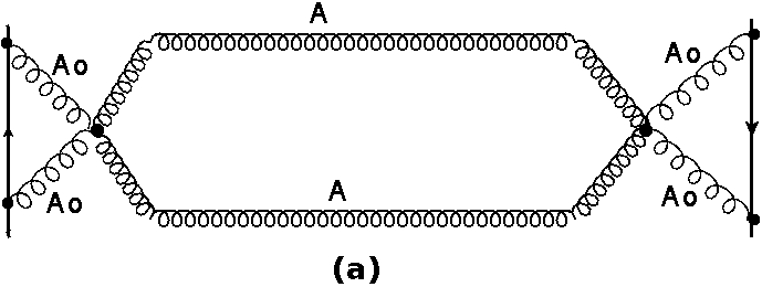
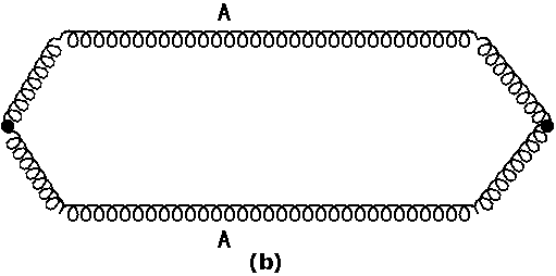
Figure 9: (a) An exchange of a pair of massive magnetic gluons between two Polyakov Loops (b) Spontaneously created gluon condensate when $\Phi=0$.

At low temperature ($T\ll T_{c}$), the amplitude of $\langle A_{0}^{2}\rangle$ is high and $\Phi\rightarrow 0$, $\Omega_{S}^{g}$ becomes

$$\Omega_{S}^{g;\;\Phi,{\bar{\Phi}}\rightarrow 0}=2T\int\frac{d^{3}p}{(2\pi)^{3}}\left[\ln\left(1-e^{-N_{c}\beta\epsilon_{g}}\right)^{2}\,\right.$$

$$\left.\!+\!\ln\left(1-e^{2\pi i/N_{c}}e^{-\beta\epsilon_{g}}\right)\!+\!\ln\left(1-e^{-2\pi i/N_{c}}e^{-\beta\epsilon_{g}}\right)\right],$$ (26)

where the color charges are frozen through color-singlet states in the confining domain. Now (26) can be viewed in the following way:

(i) The first term indicates that the Polyakov Loop confines $N_{c}$ number of spatial gluons in a same energy state representing a glueball. There are two such copies which is consistent with $SU(3)$ gauge theory as $8\otimes 8\otimes 8$ generates only two singlet glueball states. Obviously, the $Z(3)$ charge is frozen in the color singlet glueballs through the localization of $Z(3)$ charge in the global $Z(3)$ minimum in Fig. 8. The first term is negative which generates positive pressure in QCD confined object.

(ii) The remaining two spatial gluons in the second and third terms are conjugate to each other but distinguished by $Z(3)$ phase. In a confined phase ($T\ll T_{c};\ \Phi\sim 0$), Polyakov Loop disappears but this two spatial gluons cannot stay as free color charges rather they keep circulating in a closed loop of virtual color and anti-color charges as shown in the right panel of Fig. 9 in a nonperturbative vacuum. The potential combining this two spatial gluons with $Z(3)$ phases can then be written as

$$2T\int\frac{d^{3}p}{(2\pi)^{3}}\ln\left[\left(1-e^{2\pi i/N_{c}}e^{-\beta\epsilon_{g}}\right)\left(1-e^{-2\pi i/N_{c}}e^{-\beta\epsilon_{g}}\right)\right]$$

$$=2T\int\frac{d^{3}p}{(2\pi)^{3}}\ln\left(1+e^{-\beta\epsilon_{g}}+e^{-2\beta\epsilon_{g}}\right)\,,$$ (27)

which is a positive definite quantity. Such states, may be condensates, are produced spontaneously in a nonabelian gauge theory as the pressure generated by this two spatial gluons in terms of the center group $Z(3)$ is negative compared to the confined object (first term in (26)). This two gluons should not contribute directly to the thermodynamics in a confined phase. Rather they provide a nonperturbative ground state pressure which is negative and unbound from below that can be viewed as a general confining background of strong interaction. In lattice QCD calculations of equation of states this confining background is removed so that the pressure starts from zero or positive value in the confined phase (first term in (26)), i.e., in the low temperature phase ($T\ll T_{C}$).

It is also worth noting here that in Ref. [19] the two conjugate spatial gluons has been considered in the nonzero $\Phi$ domain as an exchange of a pair of massive spatial virtual gluons between two Polyakov Loops as shown in the left panel of Fig. 9. This is because Euclidean time reflection does not allow an exchange of a massless pair of spatial gluons [19]. This was shown to generate a magnetic screening mass ($\sim g^{2}T$), a solely non-perturbation correction to the electric screening mass. This in turn provides a nonperturbative mass gap to prevent those excitations of color charges having energy lower than it. In the confining phase ( $|\Phi|=0$), the Polyakov Loop disappears and this two magnetic gluons keep circulating in a closed loop that provides a confining background as discussed above.

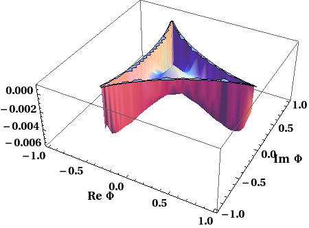
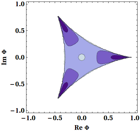
Figure 10: (color online) Left Panel: A 3D plot of full potential $\Omega=\Omega_{q}+\Omega_{\bar{q}}+\Omega_{g}\,-\,\kappa T\ln H$ in a complex $\Phi$ plane for $T=140,\,149,\,155,\,160,\,170\,\,\,{\mbox{and}}\,\,\,250$ MeV with $\mu=0$ and $\kappa=0.0075$ GeV³. Right Panel: Corresponding contour plots.

4.2 Matter sector:

The full color singlet potential in presence of matter field is given by (19) as

$$\Omega^{S}=\Omega_{q}+\Omega_{\bar{q}}+\Omega_{g}-\kappa T\ln H.$$ (28)

The $Z(3)$ symmetry with quarks and antiquarks in the full potential is explicitly broken under the rotation of $Z(3)$ since they also carry the $Z(3)$ charge. This can be viewed from Fig. 10 that displays a plot of $\Omega^{S}$ in a complex $\Phi$ plane for a set of temperatures. The left panel in Fig. 10 corresponds to 3-dimensional plots whereas right panel corresponds to contour plots in a complex $\Phi$ plane. In the range $0<T<140$ MeV, the potential has only one minimum (not shown here in Fig. 10) that apparently represents $Z(3)$ global minimum. This is because the $Z(3)$ color charges are still frozen in hadrons in the confining domain. In the temperature domain $140<T(\rm{MeV})<150$, there is still one minimum but has moved away from the $Z(3)$ center and does not remain symmetric under $Z(3)$ rotation $2\pi/3$. Here, the mean freepath of the color charges is determined by the effective size of the $Z(3)$ domains [12]. For $150\leq T(\rm{MeV})<170$, the potential shows one global minimum with larger depth and two local minima with smaller but uneven depth. This implies that all three minima are not symmetric under the $Z(3)$ rotation $2\pi/3$. This is unlike the pure gauge case in Fig. 8, an indication of explicit $Z(3)$ symmetry breaking in presence of dynamical quarks. In this region $150\leq T(\rm{MeV})<170$ the mean freepath of the color charges begin to increase as they tend to move from local minima to energetically favourable global minimum.

Interestingly, the explicit symmetry breaking due to the presence of the matter fields leads to a metastable state in the temperature range ($145\leq T(\rm{MeV})\leq 170$) and beyond which the system crosses smoothly to the deconfined phase. So, the concept of $T_{c}$ is not very well defined and lattice QCD calculations estimate it through various observable  and find in the range $(147-160)$ MeV. Our observation of $T_{c}\sim(165-170)$ MeV where the instability of the metastable minima stabilizes due to the expansion of the domains as can be seen clearly from the contour plots in the right panel of Fig. 10. Like gauge sector the depth of all three minima becomes almost symmetric for $T\geq 170$MeV as the domains expand with temperature. The color charges, irrespective of their nature, begin to reside at those minima in Fig. 10 for $T\geq 170$ MeV. These domains are separated by non-perturbative domain walls even well above $T_{c}$ because the fluctuations of the background gauge field are still nonzero. Moreover, the mean free path of the color charges becomes of the order of the effective size of these domains [12]. Since the domains expand, arround $T\geq T_{c}$ the domain size is usually smaller that corresponds to shorter wavelength appropriate for hydrodynamics to be applicable whereas the perturbative QCD may be applicable at high $T$ as the domain size increases. There will also be plenty of domains at high $T$ due to the fluctuations of the background gauge field. In the color deconfined phase these domains as well domain walls act as scattering centers that cause high energy jet to lose energy through gluon radiations and get quenched [12].

In the asymptotically high temperature ($T\gg T_{c}$), eq.(28) becomes

$$\Omega_{S}^{\Phi,{\bar{\Phi}}\rightarrow 1}\!\!\! = \!\!-2N_{f}T\int\frac{d^{3}p}{(2\pi)^{3}}\ln\left(1+e^{-\beta(\epsilon_{q}-\mu)}\right)^{N_{c}}$$ (29)

$$-2N_{f}T\int\frac{d^{3}p}{(2\pi)^{3}}\ln\left(1+e^{-\beta(\epsilon_{q}+\mu)}\right)^{N_{c}}$$

$$+\Omega_{g}^{{\rm{PL}};\Phi,{\bar{\Phi}}\rightarrow 1}\,,$$

where $N_{c}=3$. It represents the thermodynamic potential for a free colored quark, antiquark and gluon gas at high temperature, i.e, the color charges are completely ionized and reside at those minima in potential of Fig. 10 or equivalently at those maxima in color space of Figs. 1 and 5.

At low temperature ($T\ll T_{c}$), the potential with matter part can be written as

$$\Omega^{\rm{PL};\Phi,{\bar{\Phi}}\rightarrow 0} = \!\!-2N_{f}T\!\!\int\!\!\frac{d^{3}p}{(2\pi)^{3}}\ln\left(1+e^{-\beta N_{c}(\epsilon_{q}-\mu)}\right)$$ (30)

$$-2N_{f}T\!\!\int\!\!\frac{d^{3}p}{(2\pi)^{3}}\ln\left(1+e^{-\beta N_{c}(\epsilon_{q}+\mu)}\right)$$

$$+\Omega_{g}^{{\rm{PL}};\Phi,{\bar{\Phi}}\rightarrow 0}\,.$$

This represents the thermodynamic potential for a composite color singlet object containing three quarks(antiquarks) in a same color state with the same energy. So is for gluons as discussed earlier. One can also combine appropriate terms in (30) to get mesons, baryons, hybrid mesons, glueballs etc. In other words, the $SU(3)$ color singlet restriction vis-a-vis Polyakov Loop dynamically confines three colored charges in a same energy state, which finally forms a color neutral object like baryon and glueball. This is because color charges get frozen in color singlet states like hadrons in the global minimum when $T\ll T_{c}$ . This essentially boils down to the fact that the $SU(3)$ color singlet restriction vis-a-vis Polyakov Loop dynamically provides the basis for the recombination of partons for hadronisation from quark-gluon plasma when it cools down below $T_{c}$. In Refs. [6] the colorsingletness has explicitly shown to provide the natural explanation of the scaling law (of the valence partons) of the eliptic flow of the identified hadrons in heavy-ion collisions, a direct evidence of deconfined phase [22, 17].

5 Conclusion:

We show that the color singlet ensemble of a quark-gluon gas becomes equivalent to that of Polyakov Loop Model within a stationary point approximation. The calculation is based on quantum statistical mechanics with a global $SU(3)$ symmetry but considering the Haar measure at each spatial points to take into account the confinement effect. The normalized character in fundamental representation of $SU(3)$ exhibits center symmetry, $Z(3)$, of $SU(3)$ akin to Polyakov Loop. In the process, we have also obtained pure gauge potential explicitly.

The color singlet gauge potential shows center symmetry which is spontaneously broken in high temperature phase ($T\geq 270$ MeV). When matter field is added the center symmetry is found to be broken explicitly, which leads to a metastable state in the temperature domain $145\leq T(\rm{MeV})\leq 170$. The instability of the metastable state stabilizes for $T\geq 170$MeV and there are domains formed in the deconfined phase. We also discussed the phenomenological consequences of these center domains, both in pure gauge as well as with dynamical quarks, on color confining-deconfining phase transition or vice-versa in QCD, through the color singlet vis-a-vis Polyakov Loop potential. The center symmetry dictates that the confined phase appears as a color singlet object from the dynamical recombination of three partons as given in (30), plus a confining background. This would solely describe the thermodynamic properties of color singlet structures like baryon, antibaryon, meson and glueball. Most of the effects of heavy-ion collisions: non-perturbative nature of the deconfined phase, fluid nature, jet quenching, recombination of hadronization etc can be understood in terms of the center domains. More calculations in this direction are required to make quantitative predictions on the consequences of center domains in heavy-ion phenomenology.

Acknowledgment: CAI would like to acknowledge the financial support from University Grants Commission.

References

- [1] J. I. Kapusta and C. Gale, Finite-Temperature Field Theory Principles and Applications, Second Edition (Cambridge University Press, Cambridge, England, 1996)
- [2] H. Weyl, The Classical Groups (Princeton U.P., Princeton, NJ, 1946).
- [3] G. Auberson et al., J. Math. Phys. 27, 1658 (1986).
- [4] B. Müller, The Physics of Quark-Gluon Plasma, First Edition (Springer-Verlag, Berlin, Germany, 1985); K. Redlich and L. Turko, Z. Phys. C5, 201 (1980); L. Turko, Phys. Lett. B104, 153 (1981); H-T Elze and W. Greiner, Phys. Lett. B179, 385 (1986); M. I. Gorenstein et al., Phys. Lett. B123, 437 (1983); B. Skagerstam, Z. Phys. C24, 97 (1984); K. Kusaka, Phys. Lett. B269, 17 (1991); I. Zakout and C. Greiner, Phys. Rev. C78, 034916 (2008); arXiv:1107.5497 .
- [5] A. Ansari and M. G. Mustafa; Nucl. Phys. A539, 752 (1992); Phys. Rev. C55, 2005 (1997); ibid. 56, 420 (1997); M. G. Mustafa, Phys. Lett. B318, 517 (1994); Phys. Rev. D49, 4634 (1994); M.G. Mustafa, A. Sen, and L. Paria, Eur.Phys. J. C11 729 (1999).
- [6] R. Abir and M. G. Mustafa, Phys. Rev. C80, 051903 (R) (2009).
- [7] R. D. Pisarski, Phys. Rev. D62, 111501 (2000); A. Dumitru and R. D. Pisarski, Phys. Lett. B525, 95 (2002); A Dumitru and R. D. Pisarski, Phys. Rev. D66, 096003 (2002); A. Dumitru, Y. Hatta, J. Lenaghan, K. Orginos, R. D. Pisarski, Phys. Rev. D70, 034511 (2004);
- [8] D. J. Gross and R. D. Pisarski, Rev. Mod. Phys. 53 43 (1981); A. Gocksch and R. D. Pisarski, Nucl. Phys. B402, 657 (1993); N. Weiss, Phys. Rev. D24, 475 (1981); Phys. Rev. D 25, 2667 (1982).
- [9] F. Fukushima, Phys. Lett. B591, 277 (2004); Phys. Rev. D68, 045004 (2003); C. Ratti, M. A. Thaller, and W. Weise, Phys. Rev. D73, 014019; S. K. Ghosh, T. K. Mukherjee, M. G. Mustafa, and R. Ray, Phys. Rev. D 73, 114007 (2006); ibid. 77, 094024 (2008); S. Mukherjee, M. G. Mustafa, and R. Ray, ibid. 75, 094015 (2007); S. Roessner, C. Ratti, and W. Weise, Phys. Rev. D75, 034007 (2007); C. Sasaki, B. Friman, and K. Redlich, Phys. Rev. D 75 074013 (2007); A. Bhattacharyya, P. Dev, S. K. Ghosh, and R. Ray, Phys. Rev. D 82, 014021 (2010); P. Dev, A. Lahiri, and R. Ray, Phys. Rev D82, 11402 (2010); ibid 83, 014011 (2010).
- [10] P. N. Meisinger, M. C. Ogilvie, and T. R. Miller, Phys. Lett. B585, 149 (2004). P. N. Meisinger, T. R. Miller and M. C. Ogilvie, Phys. Rev. D65, 034009 (2002); P. N. Meisinger and M. C. Ogilvie, Phys. Rev. D65, 056013 (2002).
- [11] C. Sasaki and K. Redlich, Phys. Rev. D86, 014007 (2012).
- [12] M. Asakawa, S. A. Bass, and B. Müller, Phys. Rev. Lett. 110 202301 (2013).
- [13] Y. Nambu and G. Jona-Lasinio, Phys. Rev. 122, 345 (1961); ibid 124, 246 (1961).
- [14] T. Hatsuda and T. Kunihiro, Phys. Rep. 247, 221 (1994); T. Kunihiro, Phys. Lett. B 271, 395 (1991).
- [15] M. Deka, S. Digal and A. P. Mishra, Phys. Rev. D 85, 114505 (2012); S. Borsanyi, J. Danzer, Z. Fodor, C. Gattringer and A. Schmidt, J. Phys. Conf. Ser. 312, 012005 (2011);J. Danzer, C. Gattringer, S. Borsanyi and Z. Fodor, PoS LATTICE 2010, 176 (2010).
- [16] M. Cheng et al., Phys. Rev. D77, 014511 (2008).
- [17] R. Fries et al., Phys. Rev. Lett. 90, 202303 (2003); V. Greco, C. M. Ko, and P. Levai, ibid. 90, 202303 (2003).
- [18] G. Boyd et al., Nucl. Phys. B469, 419 (1996).
- [19] P. Arnold and L. G. Yaffe, Phys. Rev. D52, 7208 (1995). S. Nadkarni, Phys. Rev. D22, 3738 (1986); E. Braaten and A. Nieto, Phys. Rev. Lett. 74, 3530 (1995).
- [20] A. Bazavov et al [HotQCD Collaboration], Phys. Rev. D85, 054503 (2012); P. Petreczky, J. Phys. Conf. Ser. 402, 012036 (2012).
- [21] S. Borsanyi et al [Wuppertal-Budapest Collaboration], JHEP1009, 073 (2010).
- [22] A. Adare et al [PHENIX Collaboration], Phys. Rev. Lett. 98, 162301 (2007).