Proposal of an experimental scheme for determination of penetration depth of transverse spin current by a nonlocal spin valve

Abstract

We theoretically propose an experiment to determine the penetration depth of a transverse spin current using a nonlocal spin valve with three ferromagnetic (F) layers, where the F₁, F₂, and F₃ layers act as the spin injector, detector, and absorber, respectively. We show that the penetration depth can be evaluated by measuring the dependence of the spin signal (magnetoresistance) on the thickness of the F₃ layer.

I Introduction

There has been great deal of attention paid recently to the spin transport in nano-structured ferromagnetic materials because of their potential application to spintronics devices such as magnetic random access memory and microwave oscillators. The giant and tunnel magnetoresistance effects Baibich et al. (1988); Binasch et al. (1989); Valet and Fert (1993); Yuasa et al. (2004); Parkin et al. (2004) and spin torque effect Slonczewski (1996); Berger (1996) are key physical phenomena for the operation of these devices. The origin of these phenomena is the spin dependent electron transport, i.e., the spin current. The relaxation of the spin current in nonmagnetic (N) materials has been investigated using, for example, a nonlocal spin valve system Johnson and Silsbee (1988); Johnson (1993, 2002); Jedema et al. (2001, 2003); Kimura et al. (2006, 2007a, 2007b, 2008). In ferromagnetic (F) materials, on the other hand, we should distinguish the longitudinal and the transverse spin currents, whose spin polarizations are parallel and perpendicular to the local magnetization, and which are the origins of the magnetoresistance effect Valet and Fert (1993); Takahashi and Maekawa (2003) and the spin torque effect Slonczewski (1996); Berger (1996); Brataas et al. (2001), respectively. Compared to the extensive studies on the spin relaxation of the longitudinal spin current Valet and Fert (1993); Fert and Piraux (1999); Takahashi and Maekawa (2003); Godfrey and Johnson (2006); Bass and W. P. Pratt (2007), there have been very few studies on the spin relaxation of the transverse spin current.

The penetration depth of the transverse spin current (accumulation) is an important quantity characterizing its spatial spin relaxation Taniguchi et al. (2008a, b); Taniguchi and Imamura (2008a, b). In our previous studies Taniguchi et al. (2008a, b); Taniguchi and Imamura (2008a), we proposed that the penetration depth was evaluated by spin pumping effect Tserkovnyak et al. (2002); i.e., the creation of a pure spin current by ferromagnetic resonance (FMR), in the F/N/F trilayers. The point is that one F layer is in resonance and acts as the spin injector while the other F layer is out of resonance and acts as the spin absorber. Thus, by measuring the dependence of the FMR power spectrum of the injector on the thickness of the absorber, the penetration depth of the absorber can be evaluated. Because microfabrication is unnecessary, the FMR measurement is useful for investigating the spin relaxation. However, the choice of the F material is restricted to those that can to avoid the simultaneous resonance of the two ferromagnetic layers. Also, because the magnitude of the magnetization, as well as the FMR frequency, of the absorber increases with increasing its thickness, the FMR spectrum of the injector and absorber sometimes overlap com (a). These factors make it difficult to evaluate the penetration depth of the transverse spin current.

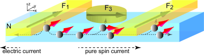
Figure 1: Schematic view of the nonlocal spin valve with three ferromagnetic (F) layers. The black arrow in each F layer represents the magnetization. The red arrow indicates the spin of the conduction electron. The electric current flows from the F₁ to the N layer while the pure spin current flows to the F₂ and F₃ layers.

In this paper, we propose an alternative method to determine the penetration depth based on the nonlocal geometry shown in Fig. 1. The three ferromagnetic layers are attached to the nonmagnetic layer, where the F₁, F₂ and F₃ layers act as the injector, detector, and absorber of the spin current. By fabricating the three F layers in different shapes, we can control the directions of the magnetization in each layer independently; thus, a noncollinear alignment of the magnetizations can be achieved. For example, in Fig. 1, the F₃ layer is assumed to be a cylinder with zero in-plane shape anisotropy; thus, the magnetization can rotate in the plane, while the magnetizations of the F₁ and F₂ layers are parallel to the stripe due to the shape anisotropy. Let us assume that the magnetization of the F₃ layer is perpendicular to those of the F₁ and F₃ layers. Then, the amount of the magnetoresistance measured in the F₂ layer depends on the absorption of the transverse spin current in the F₃ layer. Thus, by measuring the dependence of the magnetoresistance on the thickness of the F₃ layer, its penetration depth can be evaluated. There is no restriction in the choice of the materials and the change of the magnitude of the magnetization does not affect the measurement, which are advantages compared to the FMR method.

The paper is organized as follows. In Sec. II, we discuss how to calculate the spin current at each F/N interface by solving the diffusion equation of the spin accumulation. Then, the amount of the magnetoresistance in the conventional system is quantitatively estimated in Sec. III. In this section, we also show that the penetration depth of the transverse spin current can be evaluated by nonlocal geometry. Section IV provides a summary of the work. The details of the calculations are shown in the Appendix.

II Spin Current and Spin Accumulation

In this section, we show the details of the calculation of the spin current and spin accumulation in the F and N layers, which are required to evaluate the magnetoresistance effect.

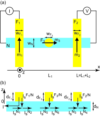
Figure 2: (a) The top and (b) side views of the system.

The details of the system we consider are schematically shown in Figs. 2 (a) and (b). The $x$ and $z$ axes are taken to be parallel and normal to the $N$ layer, whose origins are located at the F₁/N interface. The thickness and width of the F_k layer are denoted as $d_{{\rm F}_{k}}$ and $w_{{\rm F}_{k}}$ while those of the N layer are $d_{\rm N}$ and $w_{\rm N}$. The distance between the F₁ (F₂) and the F₃ layers are denoted as $L_{1}$ ($L_{2}$), respectively. The unit vector pointing in the direction of the magnetization in the F_k layer ($k=1,2,3$) is denoted as $\mathbf{m}_{k}$. The electric current, $I$, flows from the F₁ to the N layer. By passing through the F₁ layer, the conduction electrons induce spin accumulation inside and the interface of the F₁ and N layers. These spin accumulations are diffused in the N layer, creating a pure spin current into the F₂ and F₃ layers. Then, the spin accumulations are created in these F layers. It should be noted that the following formula is applicable to an arbitrary alignment of the magnetizations, $(\mathbf{m}_{1},\mathbf{m}_{2},\mathbf{m}_{3})$.

As shown in Sec. III, the magnetoresistance effect is determined by the spin current at the F/N interface. According to the spin dependent formula Brataas et al. (2001), the spin current at the F/N interface (into N, see $\mathbf{I}_{s}^{{\rm F}_{k}/{\rm N}}$ ($k=1,2,3$) in Fig. 2(b)) is given by

$$\begin{split}\mathbf{I}_{s}^{\rm F/N}\!=\!\frac{1}{4\pi}\!&\left\{\left[\frac{(1\!-\!\gamma_{\rm F/N}^{2})}{2}g_{\rm F/N}\mathbf{m}\!\cdot\!\left(\bm{\mu}_{\rm F}\!-\!\bm{\mu}_{\rm N}\right)\!+\!\frac{h}{e}\gamma_{\rm F/N}I^{\rm F/N}\right]\!\mathbf{m}\right.\\ &\!-\!g_{\rm r(F/N)}^{\uparrow\downarrow}\mathbf{m}\!\times\!\left(\bm{\mu}_{\rm N}\!\times\!\mathbf{m}\right)\!-\!g_{\rm i(F/N)}^{\uparrow\downarrow}\bm{\mu}_{\rm N}\!\times\!\mathbf{m}\\ &\!+\!\left.t_{\rm r(F/N)}^{\uparrow\downarrow}\mathbf{m}\!\times\!\left(\bm{\mu}_{\rm F}\!\times\!\mathbf{m}\right)\!+\!t_{\rm i}^{\uparrow\downarrow}\bm{\mu}_{\rm F}\!\times\!\mathbf{m}\right]\end{split}$$ (1)

where $I^{\rm F/N}$ is the electric current from the F to N layer, $g_{\rm F/N}=g^{\uparrow\uparrow}+g^{\downarrow\downarrow}$ is the sum of the spin-up and spin-down conductance, $\gamma=(g^{\uparrow\uparrow}-g^{\downarrow\downarrow})/(g^{\uparrow\uparrow}+g^{\downarrow\downarrow})$ is the spin polarization of the interface conductance Valet and Fert (1993), $g_{\rm r(i)}^{\uparrow\downarrow}$ is the real (imaginary) part of the mixing conductance Brataas et al. (2001), and $t_{\rm r(i)}^{\uparrow\downarrow}$ is the real (imaginary) part of the transmission mixing conductance Taniguchi et al. (2008a); Taniguchi and Imamura (2008a, b). The spin accumulation in the N and F layers are denoted as $\bm{\mu}_{\rm N}$ and $\bm{\mu}_{\rm F}$, respectively. The first term ($\propto\mathbf{m}$) in Eq. (1) describes the longitudinal spin transport ($\parallel\mathbf{m}$), while the other terms describe the transverse spin transport ($\perp\mathbf{m}$). The terms proportional to $g^{\uparrow\downarrow}$ describe the transverse spin injection from the N to F layer, while the terms proportional to $t^{\uparrow\downarrow}$ describe the opposite flow of the spin current. In the zero penetration depth limit, the spin accumulation in the F layer is parallel to $\mathbf{m}$, and the last two terms ($\propto t^{\uparrow\downarrow}$) in Eq. (1) can be neglected, which is assumed in Ref. Brataas et al. (2001). Although Ref. Brataas et al. (2001) assumes a spatially uniform spin accumulation, it has been shown that circuit theory is applicable to the diffusive system Bauer et al. (2003); Tserkovnyak et al. (2003).

The spin accumulation in the N layer obeys the diffusion equation Valet and Fert (1993)

$$\frac{d^{2}}{dx^{2}}\bm{\mu}_{\rm N}=\frac{1}{\lambda_{\rm N}^{2}}\bm{\mu}_{\rm N},$$ (2)

where $\lambda_{\rm N}$ is the spin diffusion length of the N layer. The solution of $\bm{\mu}_{\rm N}$ is expressed as a linear combination of $e^{\pm x/\lambda_{\rm N}}$. The spin accumulation is related to the spin current by

$$\mathbf{I}_{s}^{\rm N}=-\frac{d}{dx}\frac{\hbar S_{\rm N}\sigma_{\rm N}}{2e^{2}}\bm{\mu}_{\rm N},$$ (3)

where $S_{\rm N}=w_{\rm N}d_{\rm N}$ and $\sigma_{\rm N}$ are the cross sectional area and the conductivity of the N layer, respectively.

The longitudinal spin accumulation in the F layer, $\bm{\mu}_{\rm F}^{\rm L}=(\mathbf{m}\cdot\bm{\mu}_{\rm F})\mathbf{m}$, also obeys the diffusion equation,

$$\frac{d^{2}}{dz^{2}}\bm{\mu}_{\rm F}^{\rm L}=\frac{1}{\lambda_{\rm F}^{2}}\bm{\mu}_{\rm F}^{\rm L},$$ (4)

and its solution is expressed as a linear combination of $e^{\pm z/\lambda_{\rm F}}$, where $\lambda_{\rm F}$ is the spin diffusion length of the F layer. The longitudinal spin accumulation is related to the longitudinal spin current by

$$(\mathbf{m}\cdot\mathbf{I}_{s}^{\rm F})\mathbf{m}=-\frac{d}{dz}\frac{\hbar S_{\rm F}}{2e^{2}}\left(\sigma_{\rm F}^{\uparrow}\mu_{\rm F}^{\uparrow}-\sigma_{\rm F}^{\downarrow}\mu_{\rm F}^{\downarrow}\right)\mathbf{m},$$ (5)

where $S_{\rm F}=w_{\rm F}w_{\rm N}$ is the cross sectional area of the F layer com (b). The electrochemical potential Valet and Fert (1993) and the conductivity of the spin-$\sigma$ electron are denoted as $\mu_{\rm F}^{\sigma}$ and $\sigma_{\rm F}^{\sigma}$, respectively. The spin polarization of the conductivity is given by $\beta=(\sigma_{\rm F}^{\uparrow}-\sigma_{\rm F}^{\downarrow})/(\sigma_{\rm F}^{\uparrow}+\sigma_{\rm F}^{\downarrow})$. The resistivity is defined as $\rho_{\rm F}=1/\sigma_{\rm F}=1/(\sigma_{\rm F}^{\uparrow}+\sigma_{\rm F}^{\downarrow})$.

The transverse spin accumulation in the F layer, $\bm{\mu}_{\rm F}^{\rm T}=\mathbf{m}\times(\bm{\mu}_{\rm F}\times\mathbf{m})$ obeys the following diffusion equation Zhang et al. (2002):

$$\frac{d^{2}}{dz^{2}}\bm{\mu}_{\rm F}^{\rm T}=\frac{1}{\lambda_{J}^{2}}\bm{\mu}_{\rm F}^{\rm T}\times\mathbf{m}+\frac{1}{\lambda_{\rm F(T)}^{2}}\bm{\mu}_{\rm F}^{\rm T}.$$ (6)

The coherence length $\lambda_{J}=\sqrt{(D_{\rm F}^{\uparrow}+D_{\rm F}^{\downarrow})\hbar/(2J)}$ relates to the spin-dependent diffusion constant $D_{\rm F}^{\sigma}$ and the exchange interaction $J$ between the conduction and local electrons Zhang et al. (2002). The spin polarization of the diffusion constant is given by $\beta^{\prime}=(D_{\rm F}^{\uparrow}-D_{\rm F}^{\downarrow})/(D_{\rm F}^{\uparrow}+D_{\rm F}^{\downarrow})$. For simplicity, we assume that $\beta^{\prime}=\beta$. Then the transverse spin diffusion length $\lambda_{\rm F(T)}$ is given by $\lambda_{\rm F(T)}=\lambda_{\rm F}/\sqrt{1-\beta^{2}}$ Zhang et al. (2002). The solution of Eq. (6) is expressed as a linear combination of $e^{\pm z/\ell_{+}}$ and $e^{-\pm z/\ell_{-}}$, where

$$\frac{1}{\ell_{\pm}}=\sqrt{\frac{1}{\lambda_{\rm F(T)}^{2}}\mp\frac{i}{\lambda_{J}^{2}}}.$$ (7)

The penetration depth of the transverse spin current, $\lambda_{\rm t}$, is defined as

$$\frac{1}{\lambda_{\rm t}}={\rm Re}\left[\frac{1}{\ell_{+}}\right].$$ (8)

The transverse spin current in the F layer relates to the spin accumulation as follows:

$$\mathbf{m}\times\left(\mathbf{I}_{s}^{\rm F}\times\mathbf{m}\right)=-\frac{d}{dz}\frac{\hbar S_{\rm F}\sigma_{\rm F}^{\uparrow\downarrow}}{2e^{2}}\bm{\mu}_{\rm F}^{\rm T},$$ (9)

where $\sigma_{\rm F}^{\uparrow\downarrow}=[\sigma_{\rm F}^{\uparrow}/(1+\beta^{\prime})+\sigma_{\rm F}^{\downarrow}/(1-\beta^{\prime})]/2$.

We assume that the spin current is continuous at each F/N interface, and that the electric current is constant. Thus, the spin currents in the N layer near the interfaces, denoted as $\mathbf{I}_{s}^{{\rm N}_{i}}$ ($i=1-6$) in Fig. 2(b), should satisfy the relation $\mathbf{I}_{s}^{{\rm N}_{2k-1}}+\mathbf{I}_{s}^{{\rm F}_{k}/{\rm N}}=\mathbf{I}_{s}^{{\rm N}_{2k}}$ ($k=1,2,3$). We also assume that at the ends of the N layer, the spin current is zero. Using these boundary conditions, we can solve the diffusion equations of $\bm{\mu}_{\rm F}$ and $\bm{\mu}_{\rm N}$, where the spin current at the F/N interface can be chosen as the integral constant of the diffusion equation of the spin accumulation. Then, the spin accumulations on the right hand side of Eq. (1) can be expressed in terms of the spin currents at each F/N interface. Thus, $\mathbf{I}_{s}^{\rm F/N}$ can be obtained by solving their simultaneous equation; see Appendix A.

III Magnetoresistance

In this section, we show the details of the calculation of the magnetoresistance. Also, we show that the penetration depth of the transverse spin current of the F₃ layer can be estimated by measuring the dependence of the magnetoresistance on the thickness of the F₃ layer.

By using the spin currents at each F/N interface obtained in the previous section, the magnetoresistance measured in the F₂ layer is calculated as $R=R^{(1)}+R^{(2)}$, where $R^{(1)}$ and $R^{(2)}$ represent the contributions to the resistance from the spin dependent transports inside the F₂ layer and the interface at the F₂/N layers, respectively Valet and Fert (1993); Taniguchi et al. (2011). The explicit forms of $R^{(1)}$ and $R^{(2)}$ are given by

$$\begin{split}R^{(1)}&=-\frac{\beta_{\rm F_{2}}S_{\rm F_{2}}}{2eI}\left[\mathbf{m}_{2}\cdot\bm{\mu}_{\rm F_{2}}(z\!=\!d_{\rm F_{2}})-\mathbf{m}_{2}\cdot\bm{\mu}_{\rm F_{2}}(z\!=\!0)\right]\\ &=-\frac{\beta_{\rm F_{2}}hS_{\rm F_{2}}}{2e^{2}g_{\rm F_{2}}}\tanh\left(\frac{d_{\rm F_{2}}}{2\lambda_{\rm F_{2}}}\right)\frac{2e}{\hbar I}\mathbf{m}_{2}\cdot\mathbf{I}_{s}^{\rm F_{2}/N},\end{split}$$ (10)

$$\begin{split}R^{(2)}&=-\frac{\gamma_{\rm F_{2}/N}}{2eI}\left[S_{\rm F_{2}}\mathbf{m}_{2}\cdot\bm{\mu}_{\rm F_{2}}(z\!=\!0)-S_{\rm N}\mathbf{m}_{2}\cdot\bm{\mu}_{\rm N}(x\!=\!L)\right]\\ &=\frac{\gamma_{\rm F_{2}/N}hS_{\rm F_{2}}}{2e^{2}g_{\rm F_{2}}}\frac{1}{\tanh(d_{\rm F_{2}}/\lambda_{\rm F_{2}})}\frac{2e}{\hbar I}\mathbf{m}_{2}\cdot\mathbf{I}_{s}^{\rm F_{2}/N}\\ &\ \ \ +\frac{\gamma_{\rm F_{2}/N}hS_{\rm N}}{2e^{2}g_{\rm N}}\mathbf{m}_{2}\cdot\mathbf{I}_{s}^{\rm N{4}},\end{split}$$ (11)

where $g_{\rm F}/S_{\rm F}=h(1-\beta_{\rm F}^{2})/(2e^{2}\rho_{\rm F}\lambda_{\rm F})$ and $g_{\rm N}/S_{\rm N}=h/(2e^{2}\rho_{\rm N}\lambda_{\rm N})$, respectively. It should be noted that the above formula reproduces the results of Takahashi and Maekawa Takahashi and Maekawa (2003) by neglecting the F₃ layer and assuming that $\mathbf{m}_{1}=\pm\mathbf{m}_{2}$.

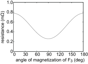
Figure 3: The dependence of the magnetoresistance on the relative angle between $\mathbf{m}_{1}$ and $\mathbf{m}_{3}$. The magnetization of the F₂ layer is parallel to $\mathbf{m}_{1}$.

Figure 3 shows an example of the calculation result using Eqs. (10) and (11). The magnetizations of the F₁ and F₂ layers are assumed to be parallel ($\mathbf{m}_{1}=\mathbf{m}_{2}$) while the magnetization of the F₃ layer changes its direction from $\mathbf{m}_{3}=\mathbf{m}_{1}$ to $\mathbf{m}_{3}=-\mathbf{m}_{1}$. The material parameters of the F₁, F₂ and F₃ layers are assumed to be identical, for simplicity, and are taken to be $\rho_{\rm F}=220$ $\Omega$nm, $\lambda_{\rm F}=5.0$ nm, $\lambda_{J}=2.8$ nm, $\beta_{\rm F}=0.35$, $\rho_{\rm N}=12$$\Omega$ nm, $\lambda_{\rm N}=1300$ nm, $R_{\rm F/N}=hS_{\rm F}/(e^{2}g_{\rm F/N})=275.4$ $\Omega$nm², $\gamma_{\rm F/N}=0.70$, $g_{\rm r(F/N)}^{\uparrow\downarrow}/S_{\rm F}=38.0$ nm^-2, $g_{\rm i(F/N)}^{\uparrow\downarrow}/S_{\rm F}=1.0$ nm^-2, $t_{\rm r(F/N)}^{\uparrow\downarrow}/S_{\rm F}=4.0$ nm^-2, $t_{\rm i(F/N)}^{\uparrow\downarrow}/S_{\rm F}=4.0$ nm^-2, $d_{\rm F}=30$ nm, $d_{\rm N}=150$ nm, $w_{\rm F_{1}}=w_{\rm F_{2}}=120$ nm, $w_{\rm F_{3}}=150$ nm, $w_{\rm N}=150$nm, $L_{1}=400$ nm, and $L_{2}=400$ nm Zhang et al. (2002); Taniguchi et al. (2008a); com (c); Fert and Piraux (1999); Bass and W. P. Pratt (2007); com (d). Then, the penetration depth is obtained as $\lambda_{\rm t}=3.5$ nm. The resistance area, Eqs. (10) and (11), is converted to resistance by using $S_{\rm F_{2}}=w_{\rm F_{2}}w_{\rm N}$, as measured in the experiment Kimura et al. (2006, 2007a, 2007b, 2008).

As shown in Fig. 3, the resistance, as well as the amounts of spin accumulation, of the parallel and antiparallel $(\mathbf{m}_{3}=\pm\mathbf{m}_{1})$ alignments are larger than those of the perpendicular alignment $(\mathbf{m}_{3}\perp\mathbf{m}_{1})$, because of the fast relaxation of the transverse spin accumulation compared to that of the longitudinal one and because of the continuity of the spin accumulation.

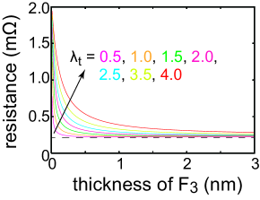
Figure 4: The dependences of the magnetoresistance on the thickness of the F₃ layer for the various penetration depth. The magnetizations of the F₂ and F₃ layers are assumed to be $\mathbf{m}_{2}\parallel\mathbf{m}_{1}$ and $\mathbf{m}_{3}\perp\mathbf{m}_{1}$, respectively. The dashed line is obtained by neglecting the transverse spin accumulation.

In Fig. 4, we show the dependences of the magnetoresistance on the thickness of the F₃ layer, $d_{\rm F_{3}}$ for various penetration depths. The values of the parameters except $d_{\rm F_{3}}$ and $\lambda_{J}$ are the same as those in Fig. 3. The penetration depth is changed by changing the value of $\lambda_{J}$, where $(\lambda_{J},\lambda_{\rm t})=$(0.7,1.0), (1.1,1.5), (1.5,2.0), (1.9,2.5), (2.3,3.0), (2.8,3.5), (3.5,4.0) nm, respectively. The magnetization alignment is assumed to be $\mathbf{m}_{2}=\mathbf{m}_{1}$ and $\mathbf{m}_{3}\perp\mathbf{m}_{1}$. The magnetoresistance decreases as the thickness of the F₃ layer increases because the amount of the spin accumulation created around the F₂ decreases due to the spin absorption in the F₃ layer. The magnetoresistance is constant for a sufficiently large thickness of $d_{\rm F_{3}}\gg\lambda_{\rm t}$. The reduction of the magnetoresistance is fast for a small $\lambda_{\rm t}$ because of the fast absorption of the spin accumulation. We also show the magnetoresistance obtained by neglecting the transverse spin accumulation. In this case, since the spin absorption in the F₃ layer occurs only at the F₃/N interface, and the amount of the spin absorption is independent of its thickness, the magnetoresistance is also independent of the thickness. In other words, the thickness dependence of the magnetoresistance reflects the relaxation of the transverse spin current in the F₃ layer. Thus, the penetration depth of the F₃ layer can be evaluated.

IV Summary

In summary, we show a theoretical formula to calculate the magnetoresistance in a nonlocal spin valve with three ferromagnetic layers. We show that the penetration depth of the transverse spin current can be evaluated by measuring the dependence of the magnetoresistance on the thickness of the spin absorber.

Appendix A: Equations to Determine Spin Currents

Here we show the details of the calculation of the spin currents at each F/N interface to evaluate Eqs. (10) and (11). First, since the magnetoresistance depends on the relative directions of the magnetizations, we introduce three sets of unit vectors, $(\mathbf{e}_{kx},\mathbf{e}_{ky},\mathbf{m}_{k})$ ($k=1,2,3$), which satisfy $\mathbf{e}_{kx}\times\mathbf{e}_{ky}=\mathbf{m}_{k}$. The rotational transformation from $(\mathbf{e}_{2x},\mathbf{e}_{2y},\mathbf{m}_{2})$ to $(\mathbf{e}_{1x},\mathbf{e}_{1y},\mathbf{m}_{1})$ is characterized by the rotation matrix $\mathsf{R}_{1}$, which depends on the two angle parameters $(\theta_{1},\varphi_{1})$ and is given by

$$\mathsf{R}_{1}=\begin{pmatrix}\cos\theta_{1}\cos\varphi_{1}&\cos\theta_{1}\sin\varphi_{1}&-\sin\theta_{1}\\ -\sin\varphi_{1}&\cos\varphi_{1}&0\\ \sin\theta_{1}\cos\varphi_{1}&\sin\theta_{1}\sin\varphi_{1}&\cos\theta_{1}\end{pmatrix}.$$ (12)

Similarly, we introduce the rotation matrix $\mathsf{R}_{3}$ which represents the relative direction of $(\mathbf{e}_{3x},\mathbf{e}_{3y},\mathbf{m}_{3})$ with respect to $(\mathbf{e}_{2x},\mathbf{e}_{2y},\mathbf{m}_{2})$ and depends on $(\theta_{3},\varphi_{3})$. Although the choice of the direction of the transverse unit vectors, $\mathbf{e}_{kx}$ and $\mathbf{e}_{ky}$, is somewhat arbitrary, the final results is independent of these choice. The relation of the longitudinal and transverse spin currents between the different F layers can be given by $(\theta_{k},\varphi_{k})$ com (e).

The general solution of the diffusion equation of the longitudinal spin accumulation is given by

$$\begin{split}\mathbf{m}\cdot\bm{\mu}_{\rm F}=\frac{4\pi}{g_{\rm F}\sinh(d_{\rm F}/\lambda_{\rm F})}&\left[\left(I_{s_{z}}^{(1)}+\frac{\hbar\beta_{\rm F}}{2e}I\right)\cosh\left(\frac{z-d_{\rm F}}{\lambda_{\rm F}}\right)\right.\\ &-\left.\left(I_{s_{z}}^{(2)}+\frac{\hbar\beta_{\rm F}}{2e}I\right)\cosh\left(\frac{z}{\lambda_{\rm F}}\right)\right],\end{split}$$ (13)

where $I_{s_{z}}^{(1)}$ and $I_{s_{z}}^{(2)}$ are the longitudinal spin current at $z=0$ and $z=d_{\rm F}$, respectively, flowing in the positive $z$ direction. In the present study, as shown in Fig. 2 (b), $I_{s_{z}}^{(1)}=-\mathbf{m}\cdot\mathbf{I}_{s}^{\rm F/N}$ and $I_{s_{z}}^{(2)}=0$. The electric current $I$ is positive for the electron flow in the positive $z$ direction, and is nonzero only in the F₁ layer. The general solution of the spin accumulation in the N layer can be obtained by replacing the quantities of the F layer in Eq. (13) with those of the N layer ($\beta$ in the N layer is zero).

Similarly, the general solution of the transverse spin accumulation is given by

$$\mathbf{e}_{x}\cdot\bm{\mu}_{\rm F}=4\pi\left[f_{1}I_{s_{x}}^{(1)}+if_{2}I_{s_{y}}^{(1)}+f_{3}I_{s_{x}}^{(2)}+if_{4}I_{s_{y}}^{(2)}\right],$$ (14)

$$\mathbf{e}_{y}\cdot\bm{\mu}_{\rm F}=4\pi\left[-if_{2}I_{s_{x}}^{(1)}+f_{1}I_{s_{y}}^{(1)}-if_{4}I_{s_{x}}^{(2)}+f_{3}I_{s_{y}}^{(2)}\right],$$ (15)

where $f_{j}(z)$ ($j=1-4$) are given by

$$f_{1}(z)={\rm Re}\left[\frac{\cosh[(z-d_{\rm F})/\ell_{+}]}{g_{\rm t}\sinh(d_{\rm F}/\ell_{+})}\right],$$ (16)

$$f_{2}(z)=i{\rm Im}\left[\frac{\cosh[(z-d_{\rm F})/\ell_{+}]}{g_{\rm t}\sinh(d_{\rm F}/\ell_{+})}\right],$$ (17)

$$f_{3}(z)=-{\rm Re}\left[\frac{\cosh(z/\ell_{+})}{g_{\rm t}\sinh(d_{\rm F}/\ell_{+})}\right],$$ (18)

$$f_{4}(z)=-i{\rm Im}\left[\frac{\cosh(z/\ell_{+})}{g_{\rm t}\sinh(d_{\rm F}/\ell_{+})}\right].$$ (19)

Here $g_{\rm t}/S_{\rm F}=[h/(4e^{2}\rho_{\rm F}\ell_{+})][(1+\beta)/(1+\beta^{\prime})+(1-\beta)/(1-\beta^{\prime})]$ Taniguchi and Imamura (2008a). $I_{s_{x}}^{(1)}$ and $I_{s_{y}}^{(1)}$ are the transverse spin current at $z=0$ while $I_{s_{x}}^{(2)}$ and $I_{s_{y}}^{(2)}$ are those at $z=d_{\rm F}$. In the present study, $I_{s_{x}}^{(1)}=-\mathbf{e}_{x}\cdot\mathbf{I}_{s}^{\rm F/N}$ and $I_{s_{y}}^{(1)}=-\mathbf{e}_{y}\cdot\mathbf{I}_{s}^{\rm F/N}$ while $I_{s_{x}}^{(2)}=I_{s_{y}}^{(2)}=0$.

By using the boundary conditions mentioned in the main text and the solutions of the spin accumulation above, we obtain the following simultaneous equations of the spin currents,

$$\mathsf{M}\mathbf{a}=\frac{\hbar I}{2e}\mathbf{s}.$$ (20)

Here, $\mathsf{M}$ is the 18^th degree coefficient matrix, whose explicit form is given in Appendix B. The 18^th degree vector $\mathbf{a}$ consists of the spin currents at each interface, and is given by $\mathbf{a}_{1}=\mathbf{m}_{1}\cdot\mathbf{I}_{s}^{\rm F_{1}/N}$, $\mathbf{a}_{2}=\mathbf{e}_{1x}\cdot\mathbf{I}_{s}^{\rm F_{1}/N}$, $\mathbf{a}_{3}=\mathbf{e}_{1y}\cdot\mathbf{I}_{s}^{\rm F_{1}/N}$, $\mathbf{a}_{4}=\mathbf{m}_{1}\cdot\mathbf{I}_{s}^{\rm N_{2}}$, $\mathbf{a}_{5}=\mathbf{e}_{1x}\cdot\mathbf{I}_{s}^{\rm N_{2}}$, $\mathbf{a}_{6}=\mathbf{e}_{1y}\cdot\mathbf{I}_{s}^{\rm N_{2}}$, $\mathbf{a}_{7}=\mathbf{m}_{2}\cdot\mathbf{I}_{s}^{\rm F_{2}/N}$, $\mathbf{a}_{8}=\mathbf{e}_{2x}\cdot\mathbf{I}_{s}^{\rm F_{2}/N}$, $\mathbf{a}_{9}=\mathbf{e}_{2y}\cdot\mathbf{I}_{s}^{\rm F_{2}/N}$, $\mathbf{a}_{10}=\mathbf{m}_{2}\cdot\mathbf{I}_{s}^{\rm N_{4}}$, $\mathbf{a}_{11}=\mathbf{e}_{2x}\cdot\mathbf{I}_{s}^{\rm N_{4}}$, $\mathbf{a}_{12}=\mathbf{e}_{2y}\cdot\mathbf{I}_{s}^{\rm N_{4}}$, $\mathbf{a}_{13}=\mathbf{m}_{3}\cdot\mathbf{I}_{s}^{\rm F_{3}/N}$, $\mathbf{a}_{14}=\mathbf{e}_{3x}\cdot\mathbf{I}_{s}^{\rm F_{3}/N}$, $\mathbf{a}_{15}=\mathbf{e}_{3y}\cdot\mathbf{I}_{s}^{\rm F_{3}/N}$, $\mathbf{a}_{16}=\mathbf{m}_{3}\cdot\mathbf{I}_{s}^{\rm N_{6}}$, $\mathbf{a}_{17}=\mathbf{e}_{3x}\cdot\mathbf{I}_{s}^{\rm N_{6}}$, $\mathbf{a}_{18}=\mathbf{e}_{3y}\cdot\mathbf{I}_{s}^{\rm N_{6}}$. The source term of the spin current and spin accumulation is given by the 18^th degree vector $\mathbf{s}$, whose non-zero component is only $\mathbf{s}_{1}$,

$$\mathbf{s}_{1}=\gamma_{\rm F_{1}/N}+\beta_{\rm F_{1}}\frac{(1-\gamma_{\rm F_{1}/N}^{2})g_{\rm F_{1}/N}}{2g_{\rm F_{1}}}\tanh\left(\frac{d_{\rm F_{1}}}{2\lambda_{\rm F_{1}}}\right).$$ (21)

Then, by numerically calculating the inverse of $\mathsf{M}$, the spin currents at each F/N interface, $\mathbf{a}$, can be obtained.

Appendix B: Explicit Form of Coefficient Matrix $\mathsf{M}$

Here we show the explicit form of the non-zero components of the coefficient matrix $\mathsf{M}$,

$$\mathsf{M}_{1,1}\!=\!1\!+\!\frac{(1-\gamma_{\rm F_{1}/N}^{2})g_{\rm F_{1}/N}}{2g_{\rm F_{1}}\tanh(d_{\rm F_{1}}/\lambda_{\rm F_{1}})}\!+\!\frac{(1-\gamma_{\rm F_{1}/N}^{2})g_{\rm F_{1}/N}}{2g_{\rm N}},$$ (22)

$$\mathsf{M}_{1,4}\!=\!-\frac{(1-\gamma_{\rm F_{1}/N}^{2})g_{\rm F_{1}/N}}{2g_{\rm N}},$$ (23)

$$\begin{split}\mathsf{M}_{2,2}\!=\!\mathsf{M}_{3,3}\!=\!&1\!+\!\frac{g_{\rm r(F_{1}/N)}^{\uparrow\downarrow}}{g_{\rm N}}\!+\!t_{\rm r(F_{1}/N)}^{\uparrow\downarrow}{\rm Re}\left[\frac{1}{g_{\rm t(F_{1})}\tanh(d_{\rm F_{1}}/\ell_{\rm F_{1}})}\right]\\ &\!+\!t_{\rm i(F_{1}/N)}^{\uparrow\downarrow}{\rm Im}\left[\frac{1}{g_{\rm t(F_{1})}\tanh(d_{\rm F_{1}}/\ell_{\rm F_{1}})}\right],\end{split}$$ (24)

$$\begin{split}\mathsf{M}_{2,3}\!=\!-\mathsf{M}_{3,2}=&\frac{g_{\rm i(F_{1}/N)}^{\uparrow\downarrow}}{g_{\rm N}}\!-\!t_{\rm r(F_{1}/N)}^{\uparrow\downarrow}{\rm Im}\left[\frac{1}{g_{\rm t(F_{1})}\tanh(d_{\rm F_{1}}/\ell_{\rm F_{1}})}\right]\\ &\!+\!t_{\rm i(F_{1}/N)}^{\uparrow\downarrow}{\rm Re}\left[\frac{1}{g_{\rm t(F_{1})}\tanh(d_{\rm F_{1}}/\ell_{\rm F_{1}})}\right],\end{split}$$ (25)

$$\mathsf{M}_{2,5}\!=\!\mathsf{M}_{3,6}\!=\!-\frac{g_{\rm r(F_{1}/N)}^{\uparrow\downarrow}}{g_{\rm N}},$$ (26)

$$\mathsf{M}_{2,6}\!=\!-\mathsf{M}_{3,5}\!=\!-\frac{g_{\rm i(F_{1}/N)}^{\uparrow\downarrow}}{g_{\rm N}},$$ (27)

$$\mathsf{M}_{4,1}\!=\!\mathsf{M}_{5,2}\!=\!\mathsf{M}_{6,3}=1,$$ (28)

$$\mathsf{M}_{4,4}\!=\!\mathsf{M}_{5,5}\!=\!\mathsf{M}_{6,6}\!=\!-\left[1\!+\!\frac{1}{\tanh(L_{1}/\lambda_{\rm N})}\right],$$ (29)

$$\mathsf{M}_{4,13}\!=\!-\mathsf{M}_{4,16}\!=\!-\frac{1}{\sinh(L_{1}/\lambda_{\rm N})}(\mathsf{R}_{1}\mathsf{R}_{3}^{-1})_{33},$$ (30)

$$\mathsf{M}_{4,14}\!=\!-\mathsf{M}_{4,17}\!=\!-\frac{1}{\sinh(L_{1}/\lambda_{\rm N})}(\mathsf{R}_{1}\mathsf{R}_{3}^{-1})_{31},$$ (31)

$$\mathsf{M}_{4,15}\!=\!-\mathsf{M}_{4,18}\!=\!-\frac{1}{\sinh(L_{1}/\lambda_{\rm N})}(\mathsf{R}_{1}\mathsf{R}_{3}^{-1})_{32},$$ (32)

$$\mathsf{M}_{5,13}\!=\!-\mathsf{M}_{5,16}\!=\!-\frac{1}{\sinh(L_{1}/\lambda_{\rm N})}(\mathsf{R}_{1}\mathsf{R}_{3}^{-1})_{13},$$ (33)

$$\mathsf{M}_{5,14}\!=\!-\mathsf{M}_{5,17}\!=\!-\frac{1}{\sinh(L_{1}/\lambda_{\rm N})}(\mathsf{R}_{1}\mathsf{R}_{3}^{-1})_{11},$$ (34)

$$\mathsf{M}_{5,15}\!=\!-\mathsf{M}_{5,18}\!=\!-\frac{1}{\sinh(L_{1}/\lambda_{\rm N})}(\mathsf{R}_{1}\mathsf{R}_{3}^{-1})_{12},$$ (35)

$$\mathsf{M}_{6,13}\!=\!-\mathsf{M}_{6,16}\!=\!-\frac{1}{\sinh(L_{1}/\lambda_{\rm N})}(\mathsf{R}_{1}\mathsf{R}_{3}^{-1})_{23},$$ (36)

$$\mathsf{M}_{6,14}\!=\!-\mathsf{M}_{6,17}\!=\!-\frac{1}{\sinh(L_{1}/\lambda_{\rm N})}(\mathsf{R}_{1}\mathsf{R}_{3}^{-1})_{21},$$ (37)

$$\mathsf{M}_{6,15}\!=\!-\mathsf{M}_{6,18}\!=\!-\frac{1}{\sinh(L_{1}/\lambda_{\rm N})}(\mathsf{R}_{1}\mathsf{R}_{3}^{-1})_{22},$$ (38)

$$\mathsf{M}_{7,7}\!=\!1\!+\!\frac{(1-\gamma_{\rm F_{2}/N}^{2})g_{\rm F_{2}/N}}{2g_{\rm F_{2}}\tanh(d_{\rm F_{2}}/\lambda_{\rm F_{2}})},$$ (39)

$$\mathsf{M}_{7,10}\!=\!\frac{(1-\gamma_{\rm F_{2}/N}^{2})g_{\rm F_{2}/N}}{2g_{\rm N}},$$ (40)

$$\begin{split}\mathsf{M}_{8,8}\!=\!\mathsf{M}_{9,9}\!=\!&1\!+\!t_{\rm r(F_{2}/N)}^{\uparrow\downarrow}{\rm Re}\left[\frac{1}{g_{\rm t(F_{2})}\tanh(d_{\rm F_{2}}/\ell_{\rm F_{2}})}\right]\\ &\!+\!t_{\rm i(F_{2}/N)}^{\uparrow\downarrow}{\rm Im}\left[\frac{1}{g_{\rm t(F_{2})}\tanh(d_{\rm F_{2}}/\ell_{\rm F_{2}})}\right],\end{split}$$ (41)

$$\begin{split}\mathsf{M}_{8,9}\!=\!-\mathsf{M}_{9,8}\!=\!&-t_{\rm r(F_{2}/N)}^{\uparrow\downarrow}{\rm Im}\left[\frac{1}{g_{\rm t(F_{2})}\tanh(d_{\rm F_{2}}/\ell_{\rm F_{2}})}\right]\\ &\!+\!t_{\rm i(F_{2}/N)}^{\uparrow\downarrow}{\rm Re}\left[\frac{1}{g_{\rm t(F_{2})}\tanh(d_{\rm F_{2}}/\ell_{\rm F_{2}})}\right],\end{split}$$ (42)

$$\mathsf{M}_{8,11}\!=\!\mathsf{M}_{9,12}\!=\!\frac{g_{\rm r(F_{2}/N)}^{\uparrow\downarrow}}{g_{\rm N}},$$ (43)

$$\mathsf{M}_{8,12}\!=\!-\mathsf{M}_{9,11}\!=\!\frac{g_{\rm i(F_{2}/N)}^{\uparrow\downarrow}}{g_{\rm N}},$$ (44)

$$\mathsf{M}_{10,7}\!=\!\mathsf{M}_{11,8}\!=\!\mathsf{M}_{12,9}\!=\!\frac{1}{\tanh(L_{2}/\lambda_{\rm N})},$$ (45)

$$\mathsf{M}_{10,10}\!=\!\mathsf{M}_{11,11}\!=\!\mathsf{M}_{12,12}=-\left[1\!+\!\frac{1}{\tanh(L_{2}/\lambda_{\rm N})}\right],$$ (46)

$$\mathsf{M}_{10,16}\!=\!\frac{1}{\sinh(L_{2}/\lambda_{\rm N})}(\mathsf{R}_{3}^{-1})_{33},$$ (47)

$$\mathsf{M}_{10,17}\!=\!\frac{1}{\sinh(L_{2}/\lambda_{\rm N})}(\mathsf{R}_{3}^{-1})_{31},$$ (48)

$$\mathsf{M}_{10,18}\!=\!\frac{1}{\sinh(L_{2}/\lambda_{\rm N})}(\mathsf{R}_{3}^{-1})_{32},$$ (49)

$$\mathsf{M}_{11,16}\!=\!\frac{1}{\sinh(L_{2}/\lambda_{\rm N})}(\mathsf{R}_{3}^{-1})_{13},$$ (50)

$$\mathsf{M}_{11,17}\!=\!\frac{1}{\sinh(L_{2}/\lambda_{\rm N})}(\mathsf{R}_{3}^{-1})_{11},$$ (51)

$$\mathsf{M}_{11,18}\!=\!\frac{1}{\sinh(L_{2}/\lambda_{\rm N})}(\mathsf{R}_{3}^{-1})_{12},$$ (52)

$$\mathsf{M}_{12,16}\!=\!\frac{1}{\sinh(L_{2}/\lambda_{\rm N})}(\mathsf{R}_{3}^{-1})_{23},$$ (53)

$$\mathsf{M}_{12,17}\!=\!\frac{1}{\sinh(L_{2}/\lambda_{\rm N})}(\mathsf{R}_{3}^{-1})_{21},$$ (54)

$$\mathsf{M}_{12,18}\!=\!\frac{1}{\sinh(L_{2}/\lambda_{\rm N})}(\mathsf{R}_{3}^{-1})_{22},$$ (55)

$$\mathsf{M}_{13,4}\!=\!\frac{(1-\gamma_{\rm F_{3}/N}^{2})g_{\rm F_{3}/N}}{2g_{\rm N}\sinh(L_{1}/\lambda_{\rm N})}(\mathsf{R}_{3}\mathsf{R}_{1}^{-1})_{33},$$ (56)

$$\mathsf{M}_{13,5}\!=\!\frac{(1-\gamma_{\rm F_{3}/N}^{2})g_{\rm F_{3}/N}}{2g_{\rm N}\sinh(L_{1}/\lambda_{\rm N})}(\mathsf{R}_{3}\mathsf{R}_{1}^{-1})_{31},$$ (57)

$$\mathsf{M}_{13,6}\!=\!\frac{(1-\gamma_{\rm F_{3}/N}^{2})g_{\rm F_{3}/N}}{2g_{\rm N}\sinh(L_{1}/\lambda_{\rm N})}(\mathsf{R}_{3}\mathsf{R}_{1}^{-1})_{32},$$ (58)

$$\mathsf{M}_{13,13}\!=\!1\!+\!\frac{(1-\gamma_{\rm F_{3}/N}^{2})g_{\rm F_{3}/N}}{2g_{\rm F_{3}}\tanh(d_{\rm F_{3}}/\lambda_{\rm F_{3}})}+\frac{(1-\gamma_{\rm F_{3}/N}^{2})g_{\rm F_{3}/N}}{2g_{\rm N}\tanh(L_{1}/\lambda_{\rm N})},$$ (59)

$$\mathsf{M}_{13,16}\!=\!-\frac{(1-\gamma_{\rm F_{3}/N}^{2})g_{\rm F_{3}/N}}{2g_{\rm N}\tanh(L_{1}/\lambda_{\rm N})},$$ (60)

$$\mathsf{M}_{14,4}\!=\!\frac{g_{\rm r(F_{3}/N)}^{\uparrow\downarrow}}{g_{\rm N}\sinh(L_{1}/\lambda_{\rm N})}(\mathsf{R}_{3}\mathsf{R}_{1}^{-1})_{13}+\frac{g_{\rm i(F_{3}/N)}^{\uparrow\downarrow}}{g_{\rm N}\sinh(L_{1}/\lambda_{\rm N})}(\mathsf{R}_{3}\mathsf{R}_{1}^{-1})_{23},$$ (61)

$$\mathsf{M}_{14,5}\!=\!\frac{g_{\rm r(F_{3}/N)}^{\uparrow\downarrow}}{g_{\rm N}\sinh(L_{1}/\lambda_{\rm N})}(\mathsf{R}_{3}\mathsf{R}_{1}^{-1})_{11}+\frac{g_{\rm i(F_{3}/N)}^{\uparrow\downarrow}}{g_{\rm N}\sinh(L_{1}/\lambda_{\rm N})}(\mathsf{R}_{3}\mathsf{R}_{1}^{-1})_{21}$$ (62)

$$\mathsf{M}_{14,6}\!=\!\frac{g_{\rm r(F_{3}/N)}^{\uparrow\downarrow}}{g_{\rm N}\sinh(L_{1}/\lambda_{\rm N})}(\mathsf{R}_{3}\mathsf{R}_{1}^{-1})_{12}+\frac{g_{\rm i(F_{3}/N)}^{\uparrow\downarrow}}{g_{\rm N}\sinh(L_{1}/\lambda_{\rm N})}(\mathsf{R}_{3}\mathsf{R}_{1}^{-1})_{22},$$ (63)

$$\mathsf{M}_{15,4}\!=\!\frac{g_{\rm r(F_{3}/N)}^{\uparrow\downarrow}}{g_{\rm N}\sinh(L_{1}/\lambda_{\rm N})}(\mathsf{R}_{3}\mathsf{R}_{1}^{-1})_{23}-\frac{g_{\rm i(F_{3}/N)}^{\uparrow\downarrow}}{g_{\rm N}\sinh(L_{1}/\lambda_{\rm N})}(\mathsf{R}_{3}\mathsf{R}_{1}^{-1})_{13},$$ (64)

$$\mathsf{M}_{15,5}\!=\!\frac{g_{\rm r(F_{3}/N)}^{\uparrow\downarrow}}{g_{\rm N}\sinh(L_{1}/\lambda_{\rm N})}(\mathsf{R}_{3}\mathsf{R}_{1}^{-1})_{21}-\frac{g_{\rm i(F_{3}/N)}^{\uparrow\downarrow}}{g_{\rm N}\sinh(L_{1}/\lambda_{\rm N})}(\mathsf{R}_{3}\mathsf{R}_{1}^{-1})_{11},$$ (65)

$$\mathsf{M}_{15,6}\!=\!\frac{g_{\rm r(F_{3}/N)}^{\uparrow\downarrow}}{g_{\rm N}\sinh(L_{1}/\lambda_{\rm N})}(\mathsf{R}_{3}\mathsf{R}_{1}^{-1})_{22}-\frac{g_{\rm i(F_{3}/N)}^{\uparrow\downarrow}}{g_{\rm N}\sinh(L_{1}/\lambda_{\rm N})}(\mathsf{R}_{3}\mathsf{R}_{1}^{-1})_{12},$$ (66)

$$\begin{split}\mathsf{M}_{14,14}\!=\!\mathsf{M}_{15,15}\!=\!&1\!+\!\frac{g_{\rm r(F_{3}/N)}^{\uparrow\downarrow}}{g_{\rm N}\tanh(L_{1}/\lambda_{\rm N})}\\ &\!+\!t_{\rm r(F_{3}/N)}^{\uparrow\downarrow}{\rm Re}\left[\frac{1}{g_{\rm t(F_{3})}\tanh(d_{\rm F_{3}}/\ell_{\rm F_{3}})}\right]\\ &\!+\!t_{\rm i(F_{3}/N)}^{\uparrow\downarrow}{\rm Im}\left[\frac{1}{g_{\rm t(F_{3})}\tanh(d_{\rm F_{3}}/\ell_{\rm F_{3}})}\right],\end{split}$$ (67)

$$\begin{split}\mathsf{M}_{14,15}\!=\!-\mathsf{M}_{15,14}\!=\!&\frac{g_{\rm i(F_{3}/N)}^{\uparrow\downarrow}}{g_{\rm N}\tanh(L_{1}/\lambda_{\rm N})}\\ &\!-\!t_{\rm r(F_{3}/N)}^{\uparrow\downarrow}{\rm Im}\left[\frac{1}{g_{\rm t(F_{3})}\tanh(d_{\rm F_{3}}/\ell_{\rm F_{3}})}\right]\\ &\!+\!t_{\rm i(F_{3}/N)}^{\uparrow\downarrow}{\rm Re}\left[\frac{1}{g_{\rm t(F_{3})}\tanh(d_{\rm F_{3}}/\ell_{\rm F_{3}})}\right],\end{split}$$ (68)

$$\mathsf{M}_{14,17}\!=\!\mathsf{M}_{15,18}\!=\!-\frac{g_{\rm r(F_{3}/N)}^{\uparrow\downarrow}}{g_{\rm N}\tanh(L_{1}/\lambda_{\rm N})},$$ (69)

$$\mathsf{M}_{14,18}\!=\!-\mathsf{M}_{15,17}\!=\!-\frac{g_{\rm i(F_{3}/N)}^{\uparrow\downarrow}}{g_{\rm N}\tanh(L_{1}/\lambda_{\rm N})},$$ (70)

$$\mathsf{M}_{16,4}\!=\!\frac{1}{\sinh(L_{1}/\lambda_{\rm N})}(\mathsf{R}_{3}\mathsf{R}_{1}^{-1})_{33},$$ (71)

$$\mathsf{M}_{16,5}\!=\!\frac{1}{\sinh(L_{1}/\lambda_{\rm N})}(\mathsf{R}_{3}\mathsf{R}_{1}^{-1})_{31},$$ (72)

$$\mathsf{M}_{16,6}\!=\!\frac{1}{\sinh(L_{1}/\lambda_{\rm N})}(\mathsf{R}_{3}\mathsf{R}_{1}^{-1})_{32},$$ (73)

$$\mathsf{M}_{17,4}\!=\!\frac{1}{\sinh(L_{1}/\lambda_{\rm N})}(\mathsf{R}_{3}\mathsf{R}_{1}^{-1})_{13},$$ (74)

$$\mathsf{M}_{17,5}\!=\!\frac{1}{\sinh(L_{1}/\lambda_{\rm N})}(\mathsf{R}_{3}\mathsf{R}_{1}^{-1})_{11},$$ (75)

$$\mathsf{M}_{17,6}\!=\!\frac{1}{\sinh(L_{1}/\lambda_{\rm N})}(\mathsf{R}_{3}\mathsf{R}_{1}^{-1})_{12},$$ (76)

$$\mathsf{M}_{18,4}\!=\!\frac{1}{\sinh(L_{1}/\lambda_{\rm N})}(\mathsf{R}_{3}\mathsf{R}_{1}^{-1})_{23},$$ (77)

$$\mathsf{M}_{18,5}\!=\!\frac{1}{\sinh(L_{1}/\lambda_{\rm N})}(\mathsf{R}_{3}\mathsf{R}_{1}^{-1})_{21},$$ (78)

$$\mathsf{M}_{18,6}\!=\!\frac{1}{\sinh(L_{1}/\lambda_{\rm N})}(\mathsf{R}_{3}\mathsf{R}_{1}^{-1})_{22},$$ (79)

$$\mathsf{M}_{16,7}\!=\!-\mathsf{M}_{16,10}\!=\!-\frac{1}{\sinh(L_{1}/\lambda_{\rm N})}(\mathsf{R}_{3})_{33},$$ (80)

$$\mathsf{M}_{16,8}\!=\!-\mathsf{M}_{16,11}\!=\!-\frac{1}{\sinh(L_{1}/\lambda_{\rm N})}(\mathsf{R}_{3})_{31},$$ (81)

$$\mathsf{M}_{16,9}\!=\!-\mathsf{M}_{16,12}\!=\!-\frac{1}{\sinh(L_{1}/\lambda_{\rm N})}(\mathsf{R}_{3})_{32},$$ (82)

$$\mathsf{M}_{17,7}\!=\!-\mathsf{M}_{17,10}\!=\!-\frac{1}{\sinh(L_{1}/\lambda_{\rm N})}(\mathsf{R}_{3})_{13},$$ (83)

$$\mathsf{M}_{17,8}\!=\!-\mathsf{M}_{17,11}\!=\!-\frac{1}{\sinh(L_{1}/\lambda_{\rm N})}(\mathsf{R}_{3})_{11},$$ (84)

$$\mathsf{M}_{17,9}\!=\!-\mathsf{M}_{17,12}\!=\!-\frac{1}{\sinh(L_{1}/\lambda_{\rm N})}(\mathsf{R}_{3})_{12},$$ (85)

$$\mathsf{M}_{18,7}\!=\!-\mathsf{M}_{18,10}\!=\!-\frac{1}{\sinh(L_{1}/\lambda_{\rm N})}(\mathsf{R}_{3})_{23},$$ (86)

$$\mathsf{M}_{18,8}\!=\!-\mathsf{M}_{18,11}\!=\!-\frac{1}{\sinh(L_{1}/\lambda_{\rm N})}(\mathsf{R}_{3})_{21},$$ (87)

$$\mathsf{M}_{18,9}\!=\!-\mathsf{M}_{18,12}\!=\!-\frac{1}{\sinh(L_{1}/\lambda_{\rm N})}(\mathsf{R}_{3})_{22},$$ (88)

$$\mathsf{M}_{16,13}\!=\!\mathsf{M}_{17,14}\!=\!\mathsf{M}_{18,15}\!=\!\frac{1}{\tanh(L_{1}/\lambda_{\rm N})},$$ (89)

$$\mathsf{M}_{16,16}\!=\!\mathsf{M}_{17,17}\!=\!\mathsf{M}_{18,18}\!=\!-\left[\frac{1}{\tanh(L_{1}/\lambda_{\rm N})}\!+\!\frac{1}{\tanh(L_{2}/\lambda_{\rm N})}\right].$$ (90)