Inflation from Strongly Coupled Gauge Dynamics

Abstract

We argue, using a phenomenological holographic approach, that walking, strongly coupled gauge theories generate a suitable potential for a small field inflation model. We show that the effective description is a model of a single inflaton. We determine the tunings necessary in the gauge sector to generate inflation and overcome the $\eta$ problem.

Inflation (see for example Lyth:1998xn ) is a key ingredient in cosmology. The usual description has a scalar field slow rolling in some suitably designed potential. Scalar fields are though technically unnatural (in the absence of supersymmetry, and putting aside the possible recent discovery of a fundamental higgs field!) but it is possible that they are an effective description of some strongly coupled symmetry breaking sector. Historically it has not been possible to directly compute in such a strongly coupled theory but the AdS/CFT Correspondence Malda ; Witten:1998qj ; Witten:1998b ; Gubser:1998bc does now allow such study.

In this paper we wish to return to the study of a model Evans:2010tf in which the inflaton is a quark anti-quark ($\bar{q}q$) bound state in a strongly coupled system. The field theory is in the spirit of QCD, breaking the quark’s chiral symmetry by the dynamical generation of a $\langle\bar{q}q\rangle$ vev, although we imagine this dynamics occurs at a much higher scale than in QCD. We consider some asymptotically free gauge theory that runs from a perturbative UV to a strongly coupled IR regime. An effective description of the strongly coupled IR will be provided by a holographic construction in the spirit of AdS/QCD Erlich:2005qh ; Da Rold:2005zs based on the D3/D7 system Polchinski ; Bertolini:2001qa ; Karch ; Mateos ; Erdmenger:2007cm . The asymptotically free UV is replaced in holographic descriptions by a conformal but still strongly coupled regime. Crucially the model includes the dynamics of chiral symmetry breaking Babington ; Ghoroku:2004sp ; Kutasov:2012uq ; Alvares:2009hv . We parameterize the running of the gauge coupling in the theory to allow us to study theories that range from near to far from conformal. For some choices of parameters we can engineer a very flat effective potential for the quark condensate. Inflation can then be obtained by placing the condensate near zero and allowing it to slow roll to the true vacuum. In the holographic dual the D7 brane rolls from a flat to a curved configuration in an AdS geometry with a particular choice of dilaton.

Naively the motion of the D7 brane, which is extended in the holographic radial direction of AdS, appears to correspond to the dynamics of a large number of coupled inflaton fields. In our previous analysis Evans:2010tf of the model we therefore resorted to a numerical computation within the DBI action for the D7 brane of the time dependent dynamics of the roll. We then numerically searched for configurations that led to longer roll times. In this paper we can present a much more clear cut understanding of the model. In particular we understand that the tuning of parameters that we used was tuning us onto the chiral restoration transition analagous to that that occurs at the edge of the conformal window in QCD Appelquist:1996dq ; Appelquist:1998rb ; Dietrich:2006cm leading to walking gauge dynamics Holdom:1981rm . This type of transition has been explored in detail using holography in Jarvinen:2009fe ; Antipin:2009dz ; Jarvinen:2011qe ; Kutasov:2012uq ; Alvares:2012kr . Further here we will show that in fact just a single eigenmode of the D7 brane, ie a single mesonic state, is playing the role of the inflaton. The model is formally equivalent to a single inflaton model. The cosmological phenomenology is then already well known Chen:2010xka . We will also address the $\eta$ problem Copeland:1994vg in the model.

It is important to stress that we will not solve any of the usual fine tunings needed in traditional inflaton models. Our aim here is simply to recast the problem for strongly coupled gauge theories and understand what those tunings imply for the running of such theories.

I The holographic description

The holographic description is based on the simplest brane construction of a 3+1d gauge theory with quarks which is the D3/D7 system ($N_{f}$ number of probe D7 branes in the background of $N_{c}$ number of D3 branes)Polchinski ; Bertolini:2001qa ; Karch ; Mateos ; Erdmenger:2007cm . See Figure 1 for the branes set-up. The basic gauge theory is large $N_{c}$, ${\cal N}=4$ super Yang-Mills with $N_{f}$ quark fields. We will work in the quenched approximation ($N_{c}\gg N_{f}$) which in the gravity dual corresponds to the probe approximation Karch . The theory has a $U(1)$ R-symmetry under which a fermionic quark anti-quark condensate has charge 2 and plays the role of $U(1)$ axial Babington .

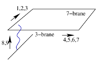
Figure 1: A sketch of the D3/D7 construction that our model is based on.

Top down models of this type exist with chiral symmetry breaking. Supergravity solutions are known that correspond to the AdS space being deformed by a running coupling introduced by a non-trivial dilaton Babington ; Ghoroku:2004sp . In cases where the coupling grows in the IR chiral symmetry breaking is induced. These models have very specific forms for the running coupling and are typically singular somewhere in the interior. A simpler and completely computable case with chiral symmetry breaking is provided by introducing a background magnetic field associated with $U(1)$ baryon number Magnetic ; Evans:2010iy . At the level of the DBI action the magnetic field term can be considered as a non-back reacted dilaton profile.

Here we will work more phenomenologically introducing a dilaton profile to induce symmetry breaking but without back reacting it on the AdS geometry Alvares:2009hv . The idea is to work in the spirit of AdS/QCD Erlich:2005qh ; Da Rold:2005zs and use different dilaton profiles to study gauge theories with different IR running. i.e. we will allow a dilaton to represent the running of the gauge theory coupling

$$e^{\Phi}=g^{2}_{\mathrm{YM}}(r)={g^{2}_{\mathrm{UV}}}~{}\beta(r)\ ,$$ (1)

where the function $\beta(r)$ will be specified in the next section with $\beta(r)\rightarrow 1$ as $r\rightarrow\infty$ ($r$ is defined in (2)).

We will take a background holographic geometry AdS₅$\times S_{5}$

$$G={1\over{g_{\mathrm{UV}}}}\left[{r^{2}\over R^{2}}(g_{tt}dt^{2}+g_{ij}dx^{i}dx^{j})\right.$$

$$\quad\left.+{R^{2}\over r^{2}}\left(d\rho^{2}+\rho^{2}d\Omega_{3}^{2}+dw_{5}^{2}+dw_{6}^{2}\right)\right]\ ,$$ (2)

where $R^{4}=4\pi{g^{2}_{\mathrm{UV}}}N_{c}\alpha^{\prime 2}$ and the second line parameterizes $\mathbb{R}^{6}$, where $\{\rho,\Omega_{3}\}$ correspond to $x^{4}$-$x^{7}$ and $w_{5(6)}$ corresponds to $x^{8(9)}$ in Figure 1. The metric $g_{tt}=-1$ and $g_{ij}=a(t)^{2}\delta_{ij}$, where $a(t)$ is the expansion factor reflecting inflation. Formally we should ask how the AdS aspects of the geometry respond to the presence of the inflation but we will leave discussion of such back reaction until the final section. As usual the radial direction $r=\sqrt{\rho^{2}+w_{5}^{2}+w_{6}^{2}}$ is the energy scale of the gauge theory.

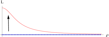
Figure 2: Evolution of the D7 brane embedding from the false vacuum ($L=0$, dotted blue line) to true vacuum ($L\neq 0$, solid red curve).

Quarks are introduced through a probe D7 brane (Fig 1). The DBI action of the D7 brane in Einstein frame is given by

$$S_{DBI}=-T_{7}\int d^{8}\xi e^{\Phi}\sqrt{-{\rm det}P[G]_{ab}}$$ (3)

where $T_{7}=1/(2\pi)^{7}\alpha^{\prime 4}$ and $P[G]_{ab}$ is the pull back of the background metric (2) onto the D7. By assuming $L=\omega_{5}(t,\vec{x},\rho)$ with $\omega_{6}=0$, we have

$$S_{DBI}=\int d^{4}x\sqrt{-g}\,\mbox{${\cal L}$}\,,$$ (4)

where

$$\frac{\mathcal{L}}{\widetilde{T}_{7}R^{4}}\equiv-\int d\rho\,\beta\,\frac{\rho^{3}}{\rho^{2}+L^{2}}\times$$

$$\qquad\sqrt{{g^{\mu\nu}\partial_{\mu}{L}\partial_{\nu}{L}+(\rho^{2}+L^{2})^{2}(1+L^{\prime 2})}}\,.$$ (5)

$\widetilde{T}_{7}=2\pi^{2}T_{7}/{g^{2}_{\mathrm{UV}}}$ and $L^{\prime}=\partial_{\rho}L$. All variables ($\rho,L$, and below $\lambda$) in the integral (5) are rescaled by $R$ and dimensionless. For the moment we leave the dilaton as an unspecified function that asymptotes to unity at large $r=\sqrt{\rho^{2}+L^{2}}$. We will consider several cases below.

Typical $t,x$ independent, vacuum configurations are easily found numerically by solving the appropriate Euler-Lagrange equation for the D7 profile $L(\rho)$. Solutions corresponding to massless quarks fall off asymptotically as

$$L\sim\frac{c}{\rho^{2}}\,,$$ (6)

with $c$ a measure of the quark condensate $\langle\bar{q}q\rangle$ and satisfy $L^{\prime}(0)=0$ Babington . There is always the symmetric $L=0$ solution but usually symmetry breaking configurations exist that curve off the $L=0$ axis as well. See Fig 2. By computing the on shell actions for both cases, we may identify which solution corresponds to the true vacuum. In this paper, we only consider the case the embedding of $L\neq 0$ corresponds to the true vacuum.

Therefore, as shown by the arrow in Figure 2, any initial embedding has to “roll down” towards the red solid curve as time goes on. This embedding dynamics is the holographic image of our field theory composite inflation dynamics. The time dependent composite inflaton may be identified with the quark condensate $c(t)=\langle\bar{q}q\rangle(t)$ in (6).

II A Flat Inflaton Potential

Our first task is to use the holographic model to find dilaton/running coupling profiles that generate a flat potential that can be used for a small field inflaton model.

In Evans:2010tf we used the step-function form for the dilaton

$$\beta=A+1-A\tanh\left[(r-\lambda)\right]\ ,$$ (7)

Here $\lambda$ is the intrinsic scale at which the conformal symmetry is broken and corresponds loosely to $\Lambda_{QCD}$ in QCD. $A$ controls the step height.

Previously Alvares:2012kr we analyzed the phase structure of such theories as a function of A. We studied the linearized action about the flat chiral symmetry preserving configuration $L=0$, $L^{\prime}=0$. If we consider $x,t$ independent configurations in (5) then we can make the change of variables

$$\tilde{\rho}=\sqrt{{1\over 2}{1\over\int_{\rho}^{\infty}{d\rho\over\beta\rho^{3}}}}\,,$$ (8)

If we write $L=\tilde{\rho}\phi$ then the action for the scalar $\phi$ is that of a canonical scalar in AdS with mass given by

$$m^{2}=-3-\delta m^{2}\,,\qquad\delta m^{2}\equiv-\beta{\rho^{5}\over\tilde{\rho}^{4}}{d\beta\over d\rho}\,.$$ (9)

Clearly our step function form for $\beta$ gives a negative contribution to the mass squared of the scalar during the range of the step. If the mass falls below the Breitenlohner-Freedman (BF) bound Breitenlohner:1982jf in AdS₅ of $m^{2}=-4$ then an instability exists. Clearly there is a critical $A$ needed to violate the BF bound. When, as is the case for this ansatz for $\beta$, the instability exists at an intermediate range of $\rho$ the transition occurs when the BF bound is violated over a sufficiently large range in $\rho$ and the transition is second order in nature.

Indeed for this ansatz if one performs the full numerical analysis one finds a second order transition from the flat embedding to a curved chiral symmetry breaking embedding at $A=0.8$. Of course as one approaches this transition the difference in energy between the flat and curved embeddings, $\Delta V$, falls to zero. Similarly the quark condensate, $\langle\bar{q}q\rangle$, also falls towards zero at the transition point. The numerical analysis of Evans:2010tf though found that as one approached the transition, rescaling $\lambda$ to keep $\Delta V$ constant, inflationary behaviour resulted. Note that keeping $\Delta V$ fixed is the appropriate way to compare inflating theories - we want the vacuum energy of the theories, which controls the expansion rate, to be the same in each case. Now we understand we are tuning to the phase transition we can make this more concrete. To achieve a very flat potential we need that the dimensionless quantity $\langle\bar{q}q\rangle/\Delta V^{3/4}$ grow as we tune to the transition point. If this is the case then the fixed drop in the potential $\Delta V$ occurs over a much larger range in the condensate and the potential becomes very flat for condensate values below the minimum.

In Fig 3a we plot $\langle\bar{q}q\rangle$ against $A$, after tuning $\lambda$ so that $\Delta V$ is the same in each case, showing that it indeed diverges as we approach the critical value of $A$. This explains why the model makes a good inflaton model.

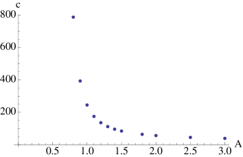
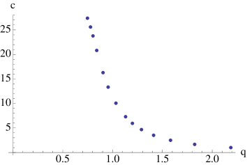
Figure 3: The quark condensate $\langle\bar{q}q\rangle$ against $A$ in the model of (7) and $q$ in (11) in each case for fixed vacuum energy $\Delta V$.

In Evans:2010tf we argued that since minimizing the step size $A$ led to inflation this suggested walking dynamics in a gauge theory might also. The holographic understanding of walking has greatly improved recently - see Jarvinen:2009fe ; Antipin:2009dz ; Jarvinen:2011qe ; Kutasov:2012uq ; Alvares:2012kr . The usual picture for a walking gauge theory is a theory lying close to the edge of the “conformal window” Appelquist:1996dq ; Appelquist:1998rb ; Dietrich:2006cm . The conformal window in QCD is a range in the number of quark flavours over which the theory is expected to be asymptotically free but approach an IR conformal fixed point. At the lower edge in the number of flavours it is presumed that the coupling value at the fixed point is sufficiently large to trigger chiral symmetry breaking. In perturbative QCD the anomalous dimension of the quark condensate is proportional to the coupling value. Schwinger Dyson analysis suggests that chiral symmetry breaking sets in when the dimension of the condensate falls to about 2 Appelquist:1988yc ; Cohen:1988sq ; Miransky:1988gk . In the holographic analysis the scalar $\phi$ we introduced below (8) is dual to the quark condensate. The naive AdS dictionary relates its mass to the dimension of the quark condensate, $\Delta$, according to $m^{2}=\Delta(\Delta-4)$. The BF bound for instability therefore again corresponds to the condensate dimension falling to 2.

The model above therefore confirms some of the the normal intuition for the onset of the chiral transition. However, the ansatz for $\beta$ in (7) does not lead to an IR fixed point for the scalar mass squared or equivalently the condensate’s anomalous dimension. Instead the extra contribution to the scalar mass (9) is only present across the step in $\beta$ where the derivative is non-zero. In Alvares:2012kr we presented a simple fix for this aspect of the quark physics which hopefully makes the dynamics closer to that of walking theories. If we set $\beta\sim 1/\rho^{q}$ in the IR then we find

$$\delta m^{2}={4q\over(2-q)^{2}}\,.$$ (10)

This form for $\beta$ ensures a fixed IR shift in the mass squared. Varying $q$ so that $m^{2}$ moves through -4 leads to a chiral phase transition which shows Miransky scaling Miransky:1996pd or BKT-like behaviour Kaplan:2009kr ; bkt ; Evans:2010hi (the condensate grows exponentially from the transition point). This behaviour is that expected at the walking edge of the conformal window.

To make a consistent model we must find a form for $\beta$ that has the required IR form but asymptotes to unity at large AdS radius. The simplest example is

$$\beta=1+{B\over r^{q}}=1+{B\over(\rho^{2}+L^{2})^{q/2}}\,.$$ (11)

It is important to stress that the chiral transition is triggered by the far IR behaviour of the ansatz and the UV extension is largely unimportant.

The choice of $\beta$ in (11) therefore provides a decent stab at describing the physics of the BKT transition at the edge of the conformal window. Does our previous supposition that these theories will generate a very flat potential suitable for inflation still hold? It is straight forward to check - we can solve the full embedding equation numerically and plot $\langle\bar{q}q\rangle$ against $q$, after tuning $B$ so that $\Delta V$ is the same in each case. We show this plot in Fig 3. We indeed again see that the condensate diverges and hence the potential becomes flat as we tune to the critical $q=0.536$. Walking dynamics and inflation again seemed to be linked in this framework.

III The Roll Dynamics

In Evans:2010tf we studied the time dependent roll of the symmetric flat D7 embedding to the symmetry breaking solution in the background of the dilaton profile in (7). We showed numerically that as the parameters approached the critical coupling described above, at fixed $\Delta V$, the roll time grew, supporting the idea that such theories will generate inflation. To set the roll moving we used an initial velocity distribution

$$\dot{L}(\rho,t=0)=ve^{-\rho^{2}}\,.$$ (12)

We found the time to reach the vacuum state was largely independent of this form although of course it does depend on the total energy injected.

Naively this model looked to us to be a multi-inflaton problem in 3+1d because of the $\rho$ dependence in the D7 profile $L(\rho,t)$ in the holographic description. Here though we will show that the model is equivalent to a single inflaton model.

III.1 Linearized Regime Analysis

At early times the brane lies close to $L(\rho)=0$ and has small $L^{\prime}(\rho)$ so it is natural to consider a linearized regime. The quadratic Lagrangian $\mbox{${\cal L}$}_{(0)}$ reads:

$$\mbox{${\cal L}$}_{(0)}=\int d\rho\ a(t)^{3}\left(\frac{\beta_{0}}{2\rho}\dot{X}^{2}-\frac{\beta_{0}\rho^{3}}{2}X^{\prime 2}-\frac{\beta_{0}^{\prime}\rho^{2}}{2}X^{2}\right)\,,$$

(13)

where

$$\beta_{0}:=A+1-A\tanh\left(\rho-\lambda\right)\,,$$

$$\beta_{0}^{\prime}=-A\,\mathrm{sech}^{2}\left(\rho-\lambda\right)\,.$$ (14)

$X=\delta L$ denotes the linear fluctuation around $L=0$. This expansion is not completely legitimate (and this is why we had not pursued it in the previous paper). The expansion may break down as $\rho\rightarrow 0$ in Eq.(13) since $X$ may not be smaller than $\rho$. Thus we are assuming either 1) $X(0)\rightarrow 0$ faster than $\rho\rightarrow 0$ at least for the slow rolling regime or 2) there is a IR cut-off $\rho_{c}$ so that $\rho_{IR}\gg X(\rho_{c})$. We will adopt the second and introduce an IR cut-off, $\rho_{c}\equiv\epsilon$ - the justification for this will be retrospective based on its success as we discuss in detail below.

The linearized equation of motion is

$$-\frac{\beta_{0}}{\rho}\frac{\partial_{t}(a^{3}\dot{X})}{a^{3}}=-(\beta_{0}\rho^{3}X^{\prime})^{\prime}+\rho^{2}\beta_{0}^{\prime}X\,.$$ (15)

We can separate variables with the ansatz $X(t,\rho)\equiv T(t)R(\rho)$ and the equation of motion reads

$$\ddot{T}+3H\dot{T}+m^{2}T=0\ ,$$ (16)

$$R^{\prime\prime}+\left(\frac{3}{\rho}+\frac{\beta_{0}^{\prime}}{\beta_{0}}\right)R^{\prime}+\left(-\frac{\beta_{0}^{\prime}}{\rho\beta_{0}}+\frac{m^{2}}{\rho^{4}}\right)R=0\,,$$ (17)

where $m^{2}$ is an arbitrary separation constant for now, but in principle will be determined by the embedding dynamics along the $\rho$-direction in the background of $\beta$. So $m^{2}$ is implicitly a function of $A,\lambda$ and can be written as

$$m^{2} = \frac{\rho}{\beta_{0}}\left(-\frac{(\beta_{0}\rho^{3}R^{\prime})^{\prime}}{R}+\rho^{2}\beta_{0}^{\prime}\right)$$ (18)

$$= \frac{\int d\rho\left(\beta_{0}\rho^{3}R^{\prime 2}+\beta_{0}^{\prime}\rho^{2}R^{2}\right)}{\int d\rho\frac{\beta_{0}}{\rho}R^{2}}\,,$$ (19)

where the first condition comes from separation of variables and the second is derived from the first and also can be understood as a completeness relations for the self-adjoint operator. Indeed the Sturm-Liouville theorem applies to (17).

$$\hat{O}R(\rho)=m^{2}w(\rho)R(\rho)\,,$$ (20)

where

$$\hat{O}R=(-\rho^{3}\beta_{0}R^{\prime})^{\prime}+\rho^{2}\beta_{0}^{\prime}R,\hskip 14.22636ptw(\rho)=\frac{\beta_{0}}{\rho}\,.$$ (21)

The natural way to proceed to the solutions is as follows: firstly one could solve (17) with $R\rightarrow 0$ at large $\rho$ and subject to $R^{\prime}(0)=0$. One would expect a tower of solutions corresponding to discrete eigenvalues $m^{2}$. One could then solve for $T(t)$ using (16). The solution of that equation is simply

$$T(t)=e^{\alpha t},\hskip 28.45274pt\alpha^{2}+3H\alpha+m^{2}=0\,.$$ (22)

$\alpha$ is positive only if $m^{2}<0$. Thus after some evolution only the unstable mode (or potentially modes) would remain in the solution.

We can not complete the program above in the linearized regime because the linearized approximation is not valid at small $\rho$. To circumvent this one has to return to the full solutions to show that the linearized approximation correctly captures the main physics of the D7’s roll and to compute $m^{2}$.

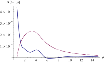
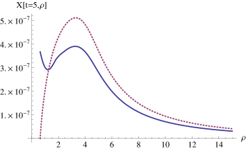
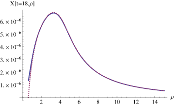
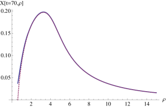
Figure 4: Evolution of full numerical embedding at different times (blue), compared with linearised solution (purple).

Let us show this procedure in a specific example. Consider the parameter set used in Evans:2010tf $A=3,\lambda=3.24$. The evolution of the embedding at times $t=1$, 5, 18 and 70 is shown in Fig. 4. From $t=5$ onwards the $\rho$ profile of the solution stabilizes (initially at $\rho>1$) which fits with a separation of variables in the solution.

Assuming that separation of variables, the function $T(t)$ may be obtained from examining the time dependence of any one point on the embedding (eg $X(t,\lambda)$). The solution to (16) is $T(t)\sim\exp(\alpha t)$. If the linearised approximation is valid, the time-derivative of the lograrithm of $T(t)$ should be a constant, $\alpha$, and that is indeed what we find. We can now determine $m^{2}$ for the most unstable mode by simply reading off the value of $\alpha$ from the exponential decay for this point. In this specific case, $\alpha=0.198$ and $m^{2}=-2.907$.

We can now perform a further consistency check. We can take this value of $m^{2}$ and plug it into (17). We then solve (17) for $R(\rho)$ numerically by shooting in from large $\rho$. By hand we cut off the solution in the IR at the point where $R(\rho)=0$ and assume that below this $\rho_{c}$ the linearized solution is not valid but also that the physics below this small $\rho$ value is not crucial to the dynamics. For example in our specific case we find

$$X=4.47\times 10^{-7}e^{0.198t}R(\rho)\ ,$$ (23)

where $R(\rho)$ is normalized as $\int^{\infty}_{\rho_{c}}wR^{2}=1$. The pre-factor is fixed by matching to the full numerics at $t=18$. We now plot these solutions (23) as the dotted curves in Figure 4. Beyond $t=17$ we have captured the full evolution very well within the linearized approximation. In particular this confirms that there is a single unstable mode that is dominating the evolution.

The embedding matches the linearized evolution until around $t=80$ which is essentially the full roll period. We also note that the peak in $R(\rho)$ is centred at $\rho=3.24$ which, as expected, is near the point $\rho=\lambda=3$ where the step change in the dilaton is found.

As a final numerical consistency check, we can evaluate $m^{2}$ from (18) and (19) numerically using our $R(\rho)$ solution. For example

$$m^{2}=\frac{\int_{\rho_{c}}^{\infty}d\rho\left(\beta_{0}\rho^{3}R^{\prime 2}+\beta_{0}^{\prime}\rho^{2}R^{2}\right)}{\int_{\rho_{c}}^{\infty}d\rho\frac{\beta_{0}}{\rho}R^{2}}=-2.907$$ (24)

from (19). The consistency is very satisfying!

In the Figure 5, we show $m^{2}$ of this inflaton mode against the parameter $A$ in (7). We change $\lambda$ in the dilaton each time to keep the vacuum energy constant. The plot again emphasizes that the best inflationary models are when we tune $A$ to its critical value.

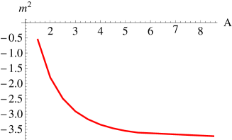
Figure 5: The mass squared of the inflaton mode in the model with a step dilaton function (7) against the step height $A$.

In principle, there are an infinite number of higher $m^{2}$ eigenvalue modes defined by (17), apart from this lowest $m^{2}$ we have found above (Strum Louiville theory enforces that the lightest state is that with no nodes which we have found). If these all have positive $m^{2}$, and hence negative $\alpha$, then their contribution to the evolution will die away exponentially fast with time (22). Could there be other sub-leading negative $m^{2}$ states though? To attempt to answer this we numerically solve (17) starting with $R(\rho_{c})=0$ and seek modes that fall to zero at large $\rho$. The resulting eigenvalues are $m^{2}=-2.907,11.18,34.49$. The unstable mode we have already discussed is the only negative mass squared state. Of course our IR boundary condition is somewhat ad hoc but the conclusion that there is just a single unstable mode seems robust to its variation.

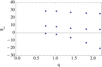
Figure 6: The lightest three mesons’ $m^{2}$ against the parameter $q$ in (11) determined from (17) with $r_{c}=0.0127$.

So far our analysis of this subsection has been for our first ansatz for $\beta$ (7). The same phenomena apply for the more sophisticated ansatz in (11). To show there is just a single inflaton state we solve (17) starting with $R(\rho_{c})=0$ and seeking modes that fall to zero at large $\rho$, but now with $\beta$ from (11). The results are $m^{2}=-10,2.495,20.08$, when $B=10,q=1,r_{c}=0.0127$. We plot the lightest three mesons’ $m^{2}$ versus the parameter $q$ of (11) in Figure 6. There is a single negative mass squared state for values of $q$ above the transition point as advertised. Again this result is robust to changes in the IR cut off.

III.2 A single effective Inflaton

Let us stress the conclusion of the analysis of the previous subsection. For the majority of the roll time in this strongly coupled gauge theory the dynamics is dominated by a single negative mass squared, linearized mode. Higher modes have positive mass and their contributions to the evolution are exponentially suppressed with time.

With a given solution $R(\rho)$ the Lagrangian (13) boils down to a standard scalar inflaton field:

$$\mbox{${\cal L}$}_{(0)}=\sqrt{-g}\left(\frac{1}{2}\dot{\phi}^{2}-\frac{1}{2}m^{2}\phi^{2}\right)\,,$$ (25)

where $\sqrt{-g}=a(t)^{3}$ and

$$\phi(t)\equiv T(t)\sqrt{\int d\rho\frac{\beta_{0}}{\rho}R(\rho)^{2}}\ .$$ (26)

Here we used (19), and discarded the boundary term.

Since the model is simply a single inflaton model the phenomenology for the bi- and tri-spectra are already well explored. For a model that provides sufficient e-folds of inflation any signal will be well below that one could hope to observe in envisaged experiments Chen:2010xka .

IV The $\eta$ problem

Inflation models are frequently beset by the so called $\eta$ problem Copeland:1994vg . One sets up a scalar potential that is tuned sufficiently flat to generate slow roll inflation. The resulting expansion term in the metric though can feedback into the inflaton potential generating a mass of order the vacuum energy H and lead to a loss of slow roll. The only solution is to further fine tune the potential so it remains flat in the presence of the back reaction. A similar problem exists in DBI inflation too as pointed out in Chen:2008hz and that mechanism is similar to how the $\eta$ problem manifests in our set up.

So far we have treated the D7 brane as a probe and neglected the effect of its back-reaction on the AdS metric, or equivalently the effect of the quarks on the ${\cal N}=4$ gauge fields. At next order the D7’s contribution to the vacuum energy should deform the AdS₅ geometry. This back-reaction in principle will induce the breaking of the SO(6) symmetry in the background geometry since the D7 does not fill the whole S⁵. That breaking has been studied in Polchinski ; Kirsch:2005uy ; Erdmenger:2011bw ; Bigazzi:2011db and induces a weak running of the gauge coupling and a Landau pole. These changes are most important in the UV and reflect the true nature of the ${\cal N}=2$ gauge theory underlying the construction. Our philosophy here is to use the IR of this model, with a phenomenological dilaton profile, to represent a wider class of gauge theories. For this reason we will neglect this particular aspect of the back-reaction. Instead we will concentrate here on the presence of the non-zero vacuum energy $\Delta V$.

The non-zero vacuum energy generates an inflating background geometry for the ${\cal N}=4$ gauge fields to live in. That breaking of conformality should change the glue dynamics and hence change the background AdS geometry. A geometry describing the ${\cal N}=4$ fields in an expanding background has been found in DeWolfe:1999cp ; Chen:2008hz and is given by

$$ds^{2}=h(r)^{2}(-dt^{2}+a(t)^{2}dx_{3}^{2})+{dr^{2}\over h(r)^{2}}+R^{2}d\Omega_{5}^{2}\,,$$ (27)

where

$$h=\sqrt{{r^{2}\over R^{2}}-H^{2}R^{2}}\,.$$ (28)

Note that at large $r$ the geometry simply returns to AdS₅. It is helpful in our context to make the change of variables

$$r={HR^{2}\over 2}\tilde{r}\left(1+{1\over\tilde{r}^{2}}\right),\quad\tilde{r}=\frac{r+\sqrt{r^{2}-H^{2}R^{4}}}{HR^{2}}\,.$$ (29)

The geometry is now of the form

$$ds^{2}=h(\tilde{r})^{2}(-dt^{2}+a(t)^{2}dx_{3}^{2})+{R^{2}\over\tilde{r}^{2}}(d\tilde{\rho}^{2}+\tilde{\rho}^{2}d\Omega_{3}^{2}+d\tilde{w}_{5}^{2}+\tilde{w}_{6}^{2})\,.$$ (30)

If we consider static embeddings of the probe D7 the DBI action is given by (4)

$$\frac{{\cal L}}{\tilde{T}_{7}R^{4}}=-\int d\tilde{\rho}\beta\frac{h^{4}}{\tilde{r}^{4}}\tilde{\rho}^{3}\sqrt{1+\tilde{L}^{{}^{\prime}2}+\frac{\dot{L}^{2}}{h^{2}}}\,.$$ (31)

Clearly the factor of $h^{4}$ changes the embeddings but we can see how to change the running dilaton/coupling to return to the critical walking scenario solutions we used above for inflation. We now require

$$\tilde{\beta} \equiv\left(\frac{2}{H}\right)^{4}\beta(\tilde{r})\frac{h^{4}}{\tilde{r}^{4}}$$ (32)

$$=\Big{(}A+1-A\tanh[(\tilde{r}-\lambda)]\Big{)}\left(1-\frac{1}{\tilde{r}^{2}}\right)^{4}\,,$$ (33)

where we normalized $\beta$ so that $\tilde{\beta}\rightarrow 1$ as $\tilde{r}\rightarrow\infty$. If we start with the initial curved embedding lying outside $\tilde{r}\gg 1$ then $\tilde{\beta}\sim\beta$ and $h\sim\tilde{r}$.

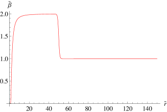
Figure 7: $\tilde{\beta}$

We will then have the same critical values of $A$ and $\lambda$ in (7) or $q$ and $B$ in (11) . At those critical points the energy difference between the symmetric flat embedding and the symmetry breaking curved embedding again falls to zero leaving a flat potential between.

We show an example plot of $\tilde{\beta}$ in the $\tilde{r}$ coordinates in Figure 7 for the case of the step function $\beta$ (7) - here we pick some representative parameters with $\Delta V<\lambda$. As shown the running has only very small variation from the previous case around the scale $\lambda$ but then large deviation at the scale $H<<\lambda$. The required form around the scale $H$ looks very peculiar and it is hard to imagine how it could be achieved in a gauge theory. In fact this is not necessary though. The potential is rather flat for all smooth configurations between the flat embedding and the true vacuum embedding. To achieve inflation we do not need to begin with a completely flat embedding that penetrates down to $r=0$. Instead we can have some initial condition that lies in the range $H<L<\lambda$ so that the brane only ever sees $\tilde{\beta}$ where it lies close to the ansatz for $\beta$ in previous sections. Such small changes from our original ansatz seem no more or less arbitrary than the original ansatz. The conclusion that walking dynamics could be responsible for inflation remains even including the back-reaction of the $\eta$ problem.

Of course we must stress here that we have not in any sense solved the fine tuning problems associated with generating inflation or solving the $\eta$ problem. These tunings are necessarily still present in our choice of dilaton profile $\beta$ (and indeed we have not tried to backreact $\beta$ on the geometry either). We hope though that we have recast those problems in an interesting fashion that teaches us about the properties of a strongly coupled gauge theory that might cause inflation.

- (1) D. H. Lyth and A. Riotto, Phys. Rept. 314 (1999) 1 [arXiv:hep-ph/9807278].
- (2) J. M. Maldacena, Adv. Theor. Math. Phys. 2, 231 (1998) Int. J. Theor. Phys. 38, 1113 (1999) [arXiv:hep-th/9711200].
- (3) E. Witten, Adv. Theor. Math. Phys. 2 (1998) 253 [arXiv:hep-th/9802150].
- (4) E. Witten, Adv. Theor. Math. Phys. 2 (1998) 505 [arXiv:hep-th/9803131].
- (5) S. S. Gubser, I. R. Klebanov and A. M. Polyakov, Phys. Lett. B 428 (1998) 105 [arXiv:hep-th/9802109].
- (6) N. Evans, J. French and K. -Y. Kim, JHEP 1011 (2010) 145 [arXiv:1009.5678 [hep-th]].
- (7) X. Chen, JCAP 1106 (2011) 012 [arXiv:1010.2851 [hep-th]].
- (8) P. Channuie, J. J. Joergensen and F. Sannino, JCAP 1105 (2011) 007 [arXiv:1102.2898 [hep-ph]].
- (9) F. Bezrukov, P. Channuie, J. J. Joergensen and F. Sannino, arXiv:1112.4054 [hep-ph].
- (10) J. Erlich, E. Katz, D. T. Son and M. A. Stephanov, Phys. Rev. Lett. 95 (2005) 261602 [arXiv:hep-ph/0501128].
- (11) L. Da Rold and A. Pomarol, Nucl. Phys. B 721 (2005) 79 [arXiv:hep-ph/0501218].
- (12) M. Grana and J. Polchinski, Phys. Rev. D65 (2002) 126005, [arXiv: hep-th/0106014].
- (13) M. Bertolini, P. Di Vecchia, M. Frau, A. Lerda and R. Marotta, Nucl. Phys. B 621, 157 (2002) [arXiv:hep-th/0107057].
- (14) A. Karch and E. Katz, JHEP 0206, 043 (2002) [arXiv:hep-th/0205236].
- (15) M. Kruczenski, D. Mateos, R. C. Myers and D. J. Winters, JHEP 0307 049, 2003 [arXiv:hep-th/0304032].
- (16) J. Erdmenger, N. Evans, I. Kirsch and E. Threlfall, arXiv:0711.4467 [hep-th].
- (17) J. Babington, J. Erdmenger, N. J. Evans, Z. Guralnik and I. Kirsch, Phys. Rev. D 69 (2004) 066007 [arXiv:hep-th/0306018].
- (18) K. Ghoroku and M. Yahiro, Phys. Lett. B 604 (2004) 235 [arXiv:hep-th/0408040].
- (19) R. Alvares, N. Evans, A. Gebauer and G. J. Weatherill, Phys. Rev. D 81 (2010) 025013 [arXiv:0910.3073 [hep-ph]].
- (20) D. Kutasov, J. Lin and A. Parnachev, Nucl. Phys. B 863 (2012) 361 [arXiv:1201.4123 [hep-th]].
- (21) T. Appelquist, J. Terning and L. C. R. Wijewardhana, Phys. Rev. Lett. 77 (1996) 1214 [hep-ph/9602385].
- (22) T. Appelquist, A. Ratnaweera, J. Terning and L. C. R. Wijewardhana, Phys. Rev. D 58 (1998) 105017 [hep-ph/9806472].
- (23) D. D. Dietrich and F. Sannino, Phys. Rev. D 75 (2007) 085018 [hep-ph/0611341].
- (24) B. Holdom, Phys. Rev. D 24 (1981) 1441.
- (25) R. Alvares, N. Evans and K. -Y. Kim, arXiv:1204.2474 [hep-ph].
- (26) M. Jarvinen and F. Sannino, JHEP 1005 (2010) 041 [arXiv:0911.2462 [hep-ph]].
- (27) O. Antipin and K. Tuominen, Mod. Phys. Lett. A 26 (2011) 2227 [arXiv:0912.0674 [hep-ph]].
- (28) M. Jarvinen and E. Kiritsis, JHEP 1203 (2012) 002 [arXiv:1112.1261 [hep-ph]].
- (29) X. Chen, Adv. Astron. 2010 (2010) 638979 [arXiv:1002.1416 [astro-ph.CO]].
- (30) E. J. Copeland, A. R. Liddle, D. H. Lyth, E. D. Stewart and D. Wands, Phys. Rev. D 49 (1994) 6410 [astro-ph/9401011].
- (31) N. Evans, K. -Y. Kim, M. Magou, Y. Seo and S. -J. Sin, arXiv:1204.5640 [hep-th].
- (32) N. Evans, A. Gebauer, M. Magou and K. -Y. Kim, J. Phys. G G 39 (2012) 054005 [arXiv:1109.2633 [hep-th]].
- (33) N. Evans, K. -Y. Kim, J. P. Shock and J. P. Shock, JHEP 1109, 021 (2011) [arXiv:1107.5053 [hep-th]].
- (34) V. G. Filev, C. V. Johnson, R. C. Rashkov and K. S. Viswanathan, JHEP 0710, 019 (2007) [arXiv:hep-th/0701001];
- (35) N. Evans, A. Gebauer, K. -Y. Kim and M. Magou, JHEP 1003, 132 (2010) [arXiv:1002.1885 [hep-th]].
- (36) N. Evans, T. Kalaydzhyan, K. -y. Kim and I. Kirsch, JHEP 1101, 050 (2011) [arXiv:1011.2519 [hep-th]].
- (37) P. Breitenlohner and D. Z. Freedman, Annals Phys. 144 (1982) 249.
- (38) T. Appelquist, K. D. Lane and U. Mahanta, Phys. Rev. Lett. 61 (1988) 1553.
- (39) A. G. Cohen and H. Georgi, Nucl. Phys. B 314 (1989) 7.
- (40) V. A. Miransky and K. Yamawaki, Mod. Phys. Lett. A 4, 129 (1989).
- (41) V. A. Miransky and K. Yamawaki, Phys. Rev. D 55 (1997) 5051 [Erratum-ibid. D 56 (1997) 3768] [hep-th/9611142].
- (42) D. B. Kaplan, J. -W. Lee, D. T. Son and M. A. Stephanov, Phys. Rev. D 80 (2009) 125005 [arXiv:0905.4752 [hep-th]].
- (43) K. Jensen, A. Karch, D. T. Son and E. G. Thompson, Phys. Rev. Lett. 105, 041601 (2010) [arXiv:1002.3159 [hep-th]];
- (44) N. Evans, A. Gebauer, K. Y. Kim and M. Magou, arXiv:1003.2694 [hep-th];
- (45) X. Chen, JCAP 0812 (2008) 009 [arXiv:0807.3191 [hep-th]].
- (46) I. Kirsch and D. Vaman, Phys. Rev. D 72 (2005) 026007 [hep-th/0505164].
- (47) J. Erdmenger, V. G. Filev and D. Zoakos, arXiv:1112.4807 [hep-th].
- (48) F. Bigazzi, A. L. Cotrone, J. Mas, D. Mayerson and J. Tarrio, Commun. Theor. Phys. 57 (2012) 364 [arXiv:1110.1744 [hep-th]].
- (49) O. DeWolfe, D. Z. Freedman, S. S. Gubser and A. Karch, Phys. Rev. D 62 (2000) 046008 [hep-th/9909134].