Missing derivative discontinuity of the exchange-correlation energy for attractive interactions: the charge Kondo effect

Abstract

We show that the energy functional of ensemble Density Functional Theory (DFT) [Perdew et al., Phys. Rev. Lett. 49, 1691 (1982)] in systems with attractive interactions is a convex function of the fractional particle number $N$ and is given by a series of straight lines joining a subset of ground-state energies. As a consequence the exchange-correlation (XC) potential is not discontinuous for all $N$. We highlight the importance of this exact result in the ensemble-DFT description of the negative-$U$ Anderson model. In the atomic limit the discontinuity of the XC potential is missing for odd $N$ while for finite hybridizations the discontinuity at even $N$ is broadened. We demonstrate that the inclusion of these properties in any approximate XC potential is crucial to reproduce the characteristic signatures of the charge-Kondo effect in the conductance and charge susceptibility.

Density functional theoryhk.1964 ; ks.1965 (DFT) provides a rigorous and computationally viable tool to calculate the electronic properties of many-particle interacting systems. In spite of the great success in a wide range of applications, its practical use is still problematic in systems with fluctuating number of particles. Popular approximations like LDA or GGA are inadequate to predict, e.g., the band gap of solids,levy ; sham the correct dissociation of heteroatomic moleculesperdew1 ; perdewchp ; hrg.2012 or the electrical conductivity of nanoscale junctions.se.2008 ; mera A conceptual advance to deal with these cases is the ensemble-DFT put forward by Perdew et al..perdew1 These authors extended the original DFT formulationhk.1964 ; ks.1965 to a fractional number $N$ of electrons, and pointed out the non-differentiability of the energy functional $E[n]$ of the density $n$ at integers $N=\int n$. Typically the discontinuity in $\partial E/\partial N$ is the difference between the ionization energy and the electron affinity since for any $N$ between two consecutive integers $M$ and $M+1$ one has

$$E(N)=(M+1-N){\cal E}_{M}+(N-M){\cal E}_{M+1},$$ (1)

i.e., $E(N)$ is a series of straight lines joining consecutive ground-state energies ${\cal E}_{M}$ of the isolated system with $M$ particles. Fig. 1 (top panel) illustrates the typical outcome of a ground state calculation of $E(N)$. It is worth recalling that the crucial hypothesis for the validity of Eq. (1) is the convexity inequality

$$\Delta_{M}\equiv{\cal E}_{M+1}+{\cal E}_{M-1}-2{\cal E}_{M}\geq 0.$$ (2)

Indeed, in this case one can show that the density matrix which minimizes the total energy is a linear combination of projection operators over the ground states with $M$ and $M+1$ particles. As discussed in Ref. perdew1, the hypothesis $\Delta_{M}\geq 0$ is certainly reasonable in systems with repulsive interactions. In contrast the convexity inequality can be violated in the attractive case. For instance in the attractive Hubbard model $\Delta_{M}$ is positive for even $M$ and negative otherwise.hu ; kulik What consequences does the break-down of Eq. (2) have in ensemble-DFT? What are the physical implications?

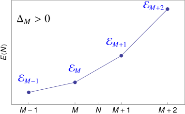
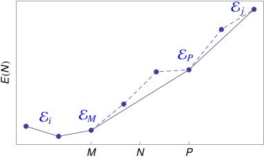
Figure 1: Illustrative examples of the total energy $E(N)$ (solid line) as a function of the fractional number $N$ when the convexity inequality (2) is (top panel) and is not (bottom panel) fulfilled. In the bottom panel the dashed line joins consecutive ground-state energies and differs from $E(N)$.

In this paper we generalize Eq. (1) to arbitrary $\Delta_{M}$. In particular we prove that $E(N)$ is a convex function given by a series of straight lines joining a subset of ground-state energies, as schematically illustrated in Fig. 1 (bottom panel). We further study the implications of the missing derivative discontinuity in the negative-$U$ Anderson model. In this prototype system the attractive interaction is at the origin of the so called charge-Kondo effect:haldane ; coleman at very low temperature the fluctuations between the empty state and the doubly-occupied state of the impurity level produce a strong enhancement of the charge susceptibility, accompanied by a drastic shrinkage of the conductance peak. We show that the key features of the charge-Kondo effect can be captured within ensemble-DFT. We extend a recently proposed functionalstef devised for the spin-Kondo effect to attractive interactions and account for the broadening of the discontinuityevers due to the finite hybridization of the impurity level. The transition from the spin-Kondo effect to the charge-Kondo effect is caused by the shift of the discontinuity of the exchange-correlation (XC) potential from $N=1$ at $U>0$lsoc.2003 ; kurth to $N=0$ and $N=2$ at $U<0$.

Theorem: Given the ground-state energies $\{{\cal E}_{I}\}$ of the isolated system with $I$ particles, if

$$\frac{{\cal E}_{I}-{\cal E}_{M}}{I-M}<\frac{{\cal E}_{P}-{\cal E}_{M}}{P-M}<\frac{{\cal E}_{J}-{\cal E}_{M}}{J-M}$$ (3)

for every $I<M$ and every $J>M$, then in the range $M<N<P$ it holds

$$E(N)=\frac{P-N}{P-M}{\cal E}_{M}+\frac{N-M}{P-M}{\cal E}_{P}.$$ (4)

Graphically this means that for $N\in[M,P]$ the energy $E(N)$ lies on the straight line connecting ${\cal E}_{M}$ to ${\cal E}_{P}$ if and only if the slope $\frac{{\cal E}_{P}-{\cal E}_{M}}{P-M}$ is larger than all the slopes of the lines connecting ${\cal E}_{M}$ to ${\cal E}_{I<M}$ and smaller than all the slopes of the lines connecting ${\cal E}_{M}$ to ${\cal E}_{J>M}$, see Fig. 1 bottom panel.

Proof: We have to show that in the range $M<N<P$ the variational energy $E_{var}(N)=\sum_{L}\omega_{L}{\cal E}_{L}$ cannot be smaller than the energy $E(N)$ in Eq. (4) for any $\{\omega_{L}\}$ constrained to satisfy

$$\sum_{L}\omega_{L}L=N,\quad\quad\sum_{L}\omega_{L}=1,$$ (5)

and $\omega_{L}\geq 0$ for all $L$. Using Eq. (3) one has

$$E_{var}(N) > \omega_{M}{\cal E}_{M}$$ (6)

$$+ \sum_{I<M}\omega_{I}\left[{\cal E}_{M}+({\cal E}_{P}-{\cal E}_{M})\frac{I-M}{P-M}\right]$$

$$+ \sum_{J>M}\omega_{J}\left[{\cal E}_{M}+({\cal E}_{P}-{\cal E}_{M})\frac{J-M}{P-M}\right]$$

$$= {\cal E}_{M}+\frac{{\cal E}_{P}-{\cal E}_{M}}{P-M}\sum_{L}\omega_{L}(L-M)=E(N),\quad\;\;$$

which proves the theorem.

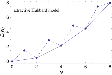
Figure 2: $E(N)$ of Eq. (4) (solid line) for the 4-sites attractive Hubbard ring with $U=-5$ and on-site energy $\varepsilon_{d}=3.5$. Energies are in units of the hopping integral. The dashed line joins consecutive ground-state energies.

Thus $E(N)$ in Eq. (4) is a convex function of $N$ and reduces to Eq. (1) provided that the convexity inequality $\Delta_{M}\geq 0$ is satisfied for all $M$ since in this case $P=M+1$. The physical content of the theorem is clear. If the system is open to a charge reservoir the density matrix at zero temperature is a mixture of ground states with $M$ and $P$ particles. For example in Fig. 2 we show that in the attractive Hubbard ring $P=M+2$, see also Refs. hu, ; kulik, . The value $P=M+2$ is peculiar of attractive systems where the electron pairing causes $\Delta_{M}\lessgtr 0$ for even/odd $M$. This property is consistent with the experimental observation of the Coulomb blockade of Cooper pairsdevoret ; gunn (Cooper staircase) in superconducting single-electron transistors, where a superconductive island is connected to metallic leads. In this situation the application of a gate voltage $v_{g}$ to the attractive region causes a jump of 2 in the number of particles at the special values $v_{g}=\frac{{\cal E}_{2M}-{\cal E}_{2M+2}}{2}$.perfetto

In ensemble-DFT the discontinuity $\partial E/\partial N$ is the sum the Kohn-Sham (KS) discontinuity, which is zero for odd $N$, and the XC discontinuity $\Delta_{\rm xc}(N)$. Since $\partial E/\partial N=0$ for odd $N$ we conclude that

$$\Delta_{\rm xc}(N)=0\quad\quad\textrm{for odd $N$}.$$ (7)

In the following, we consider a negative-$U$ Anderson model as an example in which XC discontinuity is missing. The Hamiltonian describes a set of noninteracting electrons coupled to a site at which Hubbard type interaction occurs.haldane ; coleman This is an effective model for conduction electrons coupled to an interacting impurity with vibrational modes. For strong electron-phonon coupling the polaronic shift can overcome the Coulomb charging energy and the effective electron-electron interaction turns out to be attractive. The Hamiltonian reads, in standard notation,

$$H = t\sum_{\alpha,\sigma}\sum_{i=1}^{\infty}[c^{\dagger}_{i\alpha\sigma}c_{i+1\alpha\sigma}+h.c.]+v_{g}\sum_{\sigma}n_{d\sigma}$$ (8)

$$+ Un_{d\uparrow}n_{d\downarrow}+t^{\prime}\sum_{\alpha,\sigma}[c^{\dagger}_{1\alpha\sigma}d_{\sigma}+h.c.],$$

where $t$ is the nearest-neighbour hopping in the leads, $t^{\prime}$ is the lead-impurity hopping, $U<0$ is the attractive interaction, and $v_{g}$ is the gate voltage coupled to the impurity density $n_{d\sigma}=d_{\sigma}^{{\dagger}}d_{\sigma}$. Below we focus on the half-filled system and hence take the chemical potential $\mu=0$. At very low temperature and gate voltage around $\bar{v}_{g}=-U/2=|U|/2$ this model exhibits the so called charge-Kondo effect.haldane ; coleman This effect consists in the formation of a “local pair” at the impurity and is due to strong charge fluctuations between the nearly degenerate states $|0\rangle$ and $|\uparrow\downarrow\rangle$ of the empty and doubly occupied $d$-level. As predicted by Taraphder and Colemancoleman the local pair is “screened” by the surrounding conduction electrons and forms an “isospin singlet”. With increasing $|U|$ the main features of the charge-Kondo effect are i) the shrinkage of the conductance resonance at $v_{g}=\bar{v}_{g}$ and ii) the large growth of the charge susceptibility $\chi_{d}=-\partial n_{d}/\partial v_{g}$.coleman ; mravlje These results can be qualitatively understood by mapping the Hamiltonian of Eq. (8) into the positive-$U$ Anderson model. Under a particle-hole transformation in the spin down sector, $d_{\downarrow}\rightarrow d^{{\dagger}}_{\downarrow}$ and $c_{i\alpha\downarrow}\rightarrow(-1)^{i}c^{{\dagger}}_{i\alpha\downarrow}$, the original Hamiltonian is transformed into the positive-$U$ Anderson Hamiltonian with fixed gate voltage $-|U|/2$ and effective magnetic field $B_{\mathrm{eff}}=-|U|/2+v_{g}$ coupled to $(n_{d\uparrow}-n_{d\downarrow})$.vonoppen1 ; vonoppen2 ; lopez Since the magnetic field suppresses very efficiently the Kondo correlationswiegmann ; vonoppen1 ; vonoppen2 ; mravlje ; arrachea ; cornaglia1 ; cornaglia2 the spin-Kondo effect in the transformed Hamiltonian occurs only in the proximity of $v_{g}=\bar{v}_{g}$. Consequently the conductance drops rapidly to zero as $v_{g}$ deviates from $\bar{v}_{g}$. At resonance the spin fluctuations in the transformed Hamiltonian correspond to “isospin”, i.e., charge, fluctuations in the original Hamiltonian, thus leading to the formation of an isospin singlet (local pair). This phenomenology explains the large growth of the charge susceptibility $\chi_{d}$ as $|U|$ increases (this growth is not observed for positive $U$).

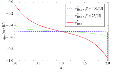
Figure 3: Potential $v^{\theta}_{\rm Hxc}$ at very low temperature, $\beta=400/|U|$, and comparison between $v^{\theta}_{\rm Hxc}$ at $\beta=1/W\gamma\approx 25/|U|$ and $v^{l}_{\rm Hxc}$ at zero temperature with $\gamma=0.125|U|$. The Lorentzian broadening is much larger than the thermal broadening for $\gamma\ll|U|$.

Let us show how these features can be captured in ensemble-DFT. In a recent Letterstef an approximate Hartree-XC potential for the positive-$U$ Anderson model was proposed. The exact energy functional of the isolated impurity reads

$$v^{\theta}_{\rm Hxc}(n_{d})=\frac{U}{2}+g(n_{d}-1),$$ (9)

where

$$g(x)=\frac{U}{2}+\frac{1}{\beta}\log\frac{x+\sqrt{x^{2}+e^{-\beta U}(1-x^{2})}}{1+x},$$ (10)

$\beta$ being the inverse temperature. For $U>0$ and in the limit $\beta\to\infty$ the potential $v^{\theta}_{\rm Hxc}(n_{d})\rightarrow U\theta(n_{d}-1)$ which has a discontinuity $U$ at $n_{d}=1$. In the Wide Band Limit Approximation (WBLA) $t,t^{\prime}\to\infty$ with constant $2t^{\prime 2}/t=\gamma\ll U$ (weak tunneling rate) one can approximate the Hartree-XC potential on the impurity $v_{\rm Hxc}\approx v_{\rm Hxc}^{\theta}$ and set it to zero in the leads.stef The discontinuity forces the occupation to be unity for gate voltages $0<v_{g}<U$.kurth ; tfsb.2005 Thus the KS potential is pinned at the Fermi energy and the KS conductance exhibits a Kondo plateau as a function of $v_{g}$.stef ; burke ; evers2

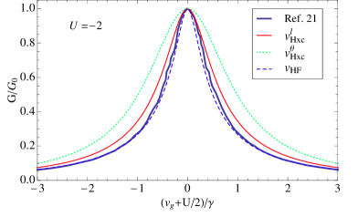
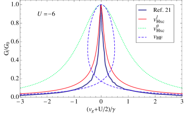
Figure 4: Conductance $G$ as a function of $v_{g}$ for two values of $U=-2,-6$ (in units of $\gamma$) and different approximation schemes. The data is compared to the variational results of Ref. mravlje, , which agree closely with the NRG data of Ref. cornaglia1, , and can be, therefore, considered as exact.

The physical argument leading to Eq. (9) is independent of the sign of $U$ and we may argue that the functional $v_{\rm Hxc}^{\theta}$ should predict, at least qualitatively, the correct conductance also for negative $U$. In the analysis below we consider the zero-temperature case. For $U<0$ the potential $v_{\rm Hxc}^{\theta}$ is not discontinuous at $n_{d}=1$ but instead develops two discontinuities (of size $|U|/2$) at $n_{d}=0$ and $n_{d}=2$, see Fig. 3.capelle Within the WBLA we determine the occupancy on the impurity by solving the self-consistent equation $n_{d}=1-\frac{2}{\pi}\tan^{-1}\!\left[\frac{v_{g}+v_{\rm Hxc}(n_{d})}{\gamma}\right]$ with $v_{\rm Hxc}=v^{\theta}_{\rm Hxc}$. Once $n_{d}$ is known we calculate the KS conductance from

$$\frac{G}{G_{0}}=\frac{\gamma^{2}}{\left[v_{g}+v_{\rm Hxc}(n_{d})\right]^{2}+\gamma^{2}},$$ (11)

where $G_{0}=1/\pi$ is the quantum of conductance. The exact KS conductance equals the exact conductance due to the Friedel sum rule and the WBLA.mera It can easily be seen that for $v_{\rm Hxc}=v^{\theta}_{\rm Hxc}$ the conductance is correctly peaked at $v_{g}=\bar{v}_{g}$ but its width is weakly dependent on $U$. Indeed $v_{\rm Hxc}^{\theta}(n_{d})=U/2$ everywhere except that at the occupations $n_{d}=0,2$, see Fig. 3. Therefore the conductance as a function of $v_{g}$ has a constant width $\gamma$ since $n_{d}$ is never exactly 0 or 2. This is illustrated in Fig. 4 where the conductance calculated using $v_{\rm Hxc}^{\theta}$ is compared with the variational results of Ref. mravlje, .

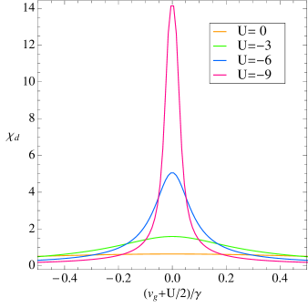
Figure 5: Charge susceptibility at the impurity $\chi_{d}=-\partial n_{d}/\partial v_{g}$ as a function of $v_{g}$ with potential $v^{l}_{\rm Hxc}$ for different values of $U$ (in units of $\gamma$).

The potential $v_{\rm Hxc}^{\theta}$ can be substantially improved by following the observation of Ref. evers, . At temperatures $T=1/\beta$ below the Kondo temperature the broadening of the discontinuity in $v_{\rm Hxc}^{\theta}$ is proportional to $\beta Ue^{-\beta U/2}$ and approaches zero in the limit $T\rightarrow 0$. However, the exact Hartree-XC potential should have an intrinsic broadening $W\sim 8\gamma/\pi|U|$ due to the finite hybridization of the impurity. Therefore we here propose a Hartree-XC potential which is the convolution of $v^{\theta}_{\rm Hxc}$ with a Lorenzian of width $W$. The resulting potential for negative $U$ and zero temperature reads

$$v_{\rm Hxc}^{l}(n_{d})=\frac{U}{2}+\frac{U}{\pi}(\arctan\frac{n_{d}-2}{W}+\arctan\frac{n_{d}}{W}).$$ (12)

In Fig. 3 we show the comparison between $v^{\theta}_{\rm Hxc}$ at finite temperature and $v^{l}_{\rm Hxc}$ at zero temperature. Choosing $\beta=1/W\gamma=\pi|U|/(8\gamma^{2})$ we see that the thermal broadening is much smaller than the Lorentzian broadening for $\gamma\ll|U|$. Figure 4 clearly illustrates the crucial role of the broadening of the discontinuity in the shrinkage of the conductance resonance as $|U|$ increases. The figure displays also the conductance in the Hartree-Fock (HF) approximation, i.e., with potential $v_{\rm HF}(n_{d})=Un_{d}/2$. Even though this potential reproduces the shrinkage up to $U\sim-2$, it becomes unreliable already for $U\sim-3$. At this critical value the self-consistent equation for the density develops multiple solutions, three in our case, as shown in the bottom panel of Fig. 4. This multistability scenario should be contrasted with the positive-$U$ Anderson model where multiple solutions within the Hartree-Fock approximation are found only out-of-equilibrium.bistab

Finally we used the Hartree-XC potential $v^{l}_{\rm Hxc}$ to calculate the charge susceptibility $\chi_{d}=-\partial n_{d}/\partial v_{g}$. In Fig. 5 we show $\chi_{d}$ as a function of $v_{g}$ for several values of $U$. Also in this case our approximation correctly captures the growth of $\chi_{d}$ at $v_{g}=\bar{v}_{g}$, another typical signature of the charge-Kondo effect. We further observe that the hight of the peak in $\chi_{d}$ saturates to values around 2 if we use the Hartree-XC potential $v^{\theta}_{\rm Hxc}$ (not shown). Thus the broadening of the discontinutity is crucial in this case as well.

In conclusion we generalized the variational energy functional of ensemble-DFT to cases where the convexity inequality is not fulfilled. The energy $E(N)$ is a convex function of the fractional particle number $N$, and it is given by the lowest series of straight lines joining a subset of ground-state energies. We discussed the relevance of this property in the description of correlated systems with attractive interactions. As for odd $N$ the energy $E(N)$ has no cusp and the KS discontinuity is zero, the XC discontinuity is zero in these cases. We showed that the missing XC discontinuity and the broadening induced by the finite hybridization with the leads are essential features of any approximate functional to describe the charge-Kondo effect in the negative-$U$ Anderson model within ensemble-DFT. The functional proposed in this work yields results in fairly good agreement with the available numerical data. In particular the shrinkage of the conductance peak as well as the growth of the charge susceptibility with increasing $|U|$ are correctly captured.

References

- (1) P. Hohenberg and W. Kohn, Phys. Rev. 136, B864 (1964).
- (2) W. Kohn and L. J. Sham, Phys. Rev. 140, A1133 (1965).
- (3) J.P. Perdew, and M. Levy, Phys. Rev. Lett. 51, 1884 (1983).
- (4) L. J. Sham and M. Schlüter, Phys. Rev. Lett. 51, 1888 (1983).
- (5) J.P. Perdew, R. G. Parr, M. Levy, and J. L. Balduz, Phys. Rev. Lett. 49, 1691 (1982).
- (6) J. P. Perdew, in Density Functional Methods in Physics, edited by R. M. Dreizler and J. da Providencia (Plenum, New York, 1985).
- (7) M. Hellgren, D. R. Rohr and E. K. U. Gross, J. Chem. Phys. 136, 034106 (2012).
- (8) P. Schmitteckert and F. Evers, Phys. Rev. Lett. 100, 086401 (2008).
- (9) H. Mera, K. Kaasbjerg, Y. M. Niquet, and G. Stefanucci, Phys. Rev. B 81, 035110 (2010).
- (10) J.-H. Hu, J.-J. Wang, G. Xianlong, M. Okumura, R. Igarashi, S. Yamada and M. Machida, Phys. Rev. B 82, 014202 (2010).
- (11) H. Boyaci, Z. Gedik and I. O. Kulik, J. Supercond. 14, 133 (2001).
- (12) F.D.M. Haldane, Phys. Rev. B 15, 281 (1977).
- (13) A. Taraphder, and P. Coleman, Phys. Rev. Lett. 66, 2814 (1991).
- (14) G. Stefanucci and S. Kurth, Phys. Rev. Lett. 107, 216401 (2011).
- (15) F. Evers and P. Schmitteckert, Phys. Chem. Chem. Phys. 13, 14417 (2011).
- (16) N. A. Lima, L. N. Oliveira and K. Capelle, Europhys. Lett. 60, 601 (2002); N. A. Lima, M. F. Silva, L. N. Oliveira and K. Capelle, Phys. Rev. Lett. 90, 146402 (2003).
- (17) S. Kurth, G. Stefanucci, E. Khosravi, C. Verdozzi, and E. K. U. Gross, Phys. Rev. Lett. 104, 236801 (2010).
- (18) T. M. Eiles, J. M. Martinis, and M. H. Devoret, Phys. Rev. Lett. 70, 1862 (1993).
- (19) K. Bladh, T. Duty, D. Gunnarsson and P. Delsing, New J. Phys. 7 180 (2005).
- (20) E. Perfetto and M. Cini, Phys. Rev. B 71, 014504 (2005).
- (21) J. Mravlje, A. Ramsǎk, and T. Rejec Phys. Rev. B 72, 121403(R) (2005).
- (22) J. Koch, M. E. Raikh, and F. von Oppen Phys. Rev. Lett. 96, 056803 (2006).
- (23) J. Koch, E. Sela, Y. Oreg, and F. von Oppen Phys. Rev. B 75, 195402 (2007).
- (24) M.-J. Hwang, M.-S. Choi, and R. López Phys. Rev. B 76, 165312 (2007).
- (25) L. Arrachea, and M.J. Rozenberg, Phys. Rev. B 72, 041301(R) (2005).
- (26) P. S. Cornaglia, D. R. Grempel, and H. Ness, Phys. Rev. Lett. 93, 147201 (2004).
- (27) P. S. Cornaglia, D. R. Grempel, and H. Ness, Phys. Rev. B 71, 075320 (2005).
- (28) P. B. Wiegmann and A. M. Tsvelick, J. Phys. C: Solid State Phys. 16 2281 (1983).
- (29) C. Toher, A. Filippetti, S. Sanvito and K. Burke, Phys. Rev. Lett. 95, 146402 (2005).
- (30) J. P. Bergfield, Z.-F Liu, K. Burke and C. A. Stafford, Phys. Rev. Lett. 108, 066801 (2012)
- (31) P. Tröster, P. Schmitteckert and F. Evers, Phys. Rev. B 85, 115409 (2012).
- (32) V. L. Campo, Jr. and K. Capelle , Phys. Rev. A 72, 061602(R) (2005).
- (33) E. Khosravi, A.-M. Uimonen, A. Stan, G. Stefanucci, S. Kurth, R. van Leeuwen and E. K. U. Gross, Phys. Rev. B 85, 075103 (2012).