Visualizing Spacetime Curvature via Frame-Drag Vortexes and Tidal Tendexes
III. Quasinormal Pulsations of Schwarzschild and Kerr Black Holes

Abstract

In recent papers, we and colleagues have introduced a way to visualize the full vacuum Riemann curvature tensor using frame-drag vortex lines and their vorticities, and tidal tendex lines and their tendicities. We have also introduced the concepts of horizon vortexes and tendexes and 3-D vortexes and tendexes (regions on or outside the horizon where vorticities or tendicities are large). In this paper, using these concepts, we discover a number of previously unknown features of quasinormal modes of Schwarzschild and Kerr black holes. These modes can be classified by a radial quantum number $n$, spheroidal harmonic orders $(l,m)$, and parity, which can be electric [$(-1)^{l}$] or magnetic [$(-1)^{l+1}$]. Among our discoveries are these: (i) There is a near duality between modes of the same $(n,l,m)$: a duality in which the tendex and vortex structures of electric-parity modes are interchanged with the vortex and tendex structures (respectively) of magnetic-parity modes. (ii) This near duality is perfect for the modes’ complex eigenfrequencies (which are well known to be identical) and perfect on the horizon; it is slightly broken in the equatorial plane of a non-spinning hole, and the breaking becomes greater out of the equatorial plane, and greater as the hole is spun up; but even out of the plane for fast-spinning holes, the duality is surprisingly good. (iii) Electric-parity modes can be regarded as generated by 3-D tendexes that stick radially out of the horizon. As these “longitudinal,” near-zone tendexes rotate or oscillate, they generate longitudinal-transverse near-zone vortexes and tendexes, and outgoing and ingoing gravitational waves. The ingoing waves act back on the longitudinal tendexes, driving them to slide off the horizon, which results in decay of the mode’s strength. (iv) By duality, magnetic-parity modes are driven in this same manner by longitudinal, near-zone vortexes that stick out of the horizon. (v) When visualized, the 3-D vortexes and tendexes of a $(l,m)=(2,2)$ mode, and also a $(2,1)$ mode, spiral outward and backward like water from a whirling sprinkler, becoming outgoing gravitational waves. By contrast, a $(2,2)$ mode superposed on a $(2,-2)$ mode, has oscillating horizon vortexes or tendexes that eject 3-dimensional vortexes and tendexes, which propagate outward becoming gravitational waves; and so does a $(2,0)$ mode. (vi) For magnetic-parity modes of a Schwarzschild black hole, the perturbative frame-drag field, and hence also the perturbative vortexes and vortex lines, are strictly gauge invariant (unaffected by infinitesimal magnetic-parity changes of time slicing and spatial coordinates). (vii) We have computed the vortex and tendex structures of electric-parity modes of Schwarzschild in two very different gauges and find essentially no discernible differences in their pictorial visualizations. (viii) We have compared the vortex lines, from a numerical-relativity simulation of a black hole binary in its final ringdown stage, with the vortex lines of a (2,2) electric-parity mode of a Kerr black hole with the same spin ($a/M=0.945$) and find remarkably good agreement.

I Motivations, Foundations and Overview

I.1 Motivations

This is the third in a series of papers that introduce a new set of tools for visualizing the Weyl curvature tensor (which, in vacuum, is the same as the Riemann tensor), and that develop, explore, and exploit these tools.

We gave a brief overview of these new tools and their applications in an initial Physical Review Letter Owen et al. (2011). Our principal motivation for these tools was described in that Letter, and in greater detail in Sec. I of our first long, pedagogical paper Nichols et al. (2011) (Paper I). In brief: We are motivated by the quest to understand the nonlinear dynamics of curved spacetime (what John Wheeler has called geometrodynamics).

The most promising venue, today, for probing geometrodynamics is numerical simulations of the collisions and mergers of binary black holes Centrella et al. (2010). Our new tools provide powerful ways to visualize the results of those simulations. As a byproduct, our visualizations may motivate new ways to compute the gravitational waveforms emitted in black-hole mergers—waveforms that are needed as templates in LIGO’s searches for and interpretation of those waves.

We will apply our tools to black-hole binaries in Paper IV of this series. But first, in Papers I–III, we are applying our tools to analytically understood spacetimes, with two goals: (i) to gain intuition into the relationships between our tools’ visual pictures of the vacuum Riemann tensor and the analytics, and (ii) to gain substantial new insights into phenomena that were long thought to be well understood. Specifically, in Paper I Nichols et al. (2011), after introducing our tools, we applied them to weak-gravity situations (“linearized theory”); in Paper II Zhang et al. (2012), we applied them to stationary (Schwarzschild and Kerr) black holes; and here in Paper III we will apply them to weak perturbations (quasinormal modes) of stationary black holes.

I.2 Our new tools, in brief

In this section, we briefly summarize our new tools. For details, see Secs. II, III, and IV of Paper I Nichols et al. (2011), and Secs. II and III of Paper II Zhang et al. (2012).

When spacetime is foliated by a family of spacelike hypersurfaces (surfaces on which some time function $t$ is constant), the electromagnetic field tensor $F_{\mu\nu}$ splits up into an electric field $E_{\hat{i}}=F_{\hat{i}\hat{0}}$ and a magnetic field $B_{\hat{i}}=\frac{1}{2}\epsilon_{\hat{i}\hat{j}\hat{k}}F_{\hat{j}\hat{k}}$, which are 3-vector fields living in the spacelike hypersurfaces. Here the indices are components in proper reference frames (orthonormal tetrads) of observers who move orthogonally to the hypersurfaces, and $\epsilon_{\hat{i}\hat{j}\hat{k}}$ is the Levi-Civita tensor in those hypersurfaces.

Similarly, the Weyl (and vacuum Riemann) tensor $C_{\mu\nu\lambda\rho}$ splits up into: (i) a tidal field $\mathcal{E}_{\hat{i}\hat{j}}=C_{\hat{i}\hat{0}\hat{j}\hat{0}}$, which produces the tidal gravitational accelerations that appear, e.g., in the equation of geodesic deviation, $\Delta a_{\hat{j}}=-\mathcal{E}_{\hat{j}\hat{k}}\Delta x^{\hat{k}}$ [Eq. (3.3) of Paper I]; and (ii) a frame-drag field $\mathcal{B}_{\hat{i}\hat{j}}=\frac{1}{2}\epsilon_{\hat{i}\hat{p}\hat{q}}C_{\hat{j}\hat{0}\hat{p}\hat{q}}$, which produces differential frame-dragging (differential precession of gyroscopes), $\Delta\Omega_{\hat{j}}=\mathcal{B}_{\hat{j}\hat{k}}\Delta x^{\hat{k}}$ [Eq. (3.11) of Paper I].

We visualize the tidal field $\bm{\mathcal{E}}$ by the integral curves of its three eigenvector fields, which we call tendex lines, and also by the eigenvalue of each tendex line, which we call the tendicity of the line and we depict using colors. Similarly, we visualize the frame-drag field $\bm{\mathcal{B}}$ by frame-drag vortex lines (integral curves of its three eigenvector fields) and their vorticities (eigenvalues, color coded). See Figs. 2 and 3 below for examples. Tendex and vortex lines are analogs of electric and magnetic field lines. Whereas through each point in space there pass just one electric and one magnetic field line, through each point pass three orthogonal tendex lines and three orthogonal vortex lines, which identify the three principal axes of $\bm{\mathcal{E}}$ and $\bm{\mathcal{B}}$.

A person whose body is oriented along a tendex line gets stretched or squeezed with a relative head-to-foot gravitational acceleration that is equal to the person’s height times the line’s tendicity (depicted blue [dark gray] in our figures for squeezing [positive tendicity] and red [light gray] for stretching [negative tendicity]). Similarly, if the person’s body is oriented along a vortex line, a gyroscope at her feet precesses around her body axis, relative to inertial frames at her head, with an angular velocity equal to her height times the line’s vorticity (depicted blue [dark gray] for clockwise precession [positive vorticity] and red [light gray] for counterclockwise [negative vorticity]).

We color code the horizon of a black hole by the normal-normal component of the tidal field, $\mathcal{E}_{NN}$, to which we give the name horizon tendicity, and also by the normal-normal component of the frame-drag field, $\mathcal{B}_{NN}$, the horizon vorticity; see, e.g., Fig. 9 below. These quantities are boost-invariant along the normal direction $\bf N$ to the horizon in the foliation’s hypersurfaces.

A person hanging radially above the horizon or falling into it experiences head-to foot squeezing (relative acceleration) equal to the horizon tendicity times the person’s height, and a differential head-to-foot precession of gyroscopes around the person’s body axis with an angular velocity equal to the horizon vorticity times the person’s height.

For any black hole, static or dynamic, the horizon tendicity $\mathcal{E}_{NN}$ and vorticity $\mathcal{B}_{NN}$ are related to the horizon’s Newman-Penrose Weyl scalar $\Psi_{2}$, and its scalar intrinsic curvature $\mathcal{R}$ and scalar extrinsic curvature $\mathcal{X}$ by

$$\mathcal{E}_{NN}+i\mathcal{B}_{NN}=2\Psi_{2}=-\frac{1}{2}(\mathcal{R}+i\mathcal{X})+2(\mu\rho-\lambda\sigma)\;;$$ (1)

Penrose and Rindler (1992), and Sec. III of Zhang et al. (2012). Here $\rho$, $\sigma$, $\mu$, $\lambda$ are spin coefficients related to the expansion and shear of the null vectors $\vec{l}$ and $\vec{n}$ used in the Newman-Penrose formalism [with $(\vec{l}+\vec{n})/\sqrt{2}=\vec{u}$ the normal to the foliation’s hypersurfaces, $(\vec{l}-\vec{n})/\sqrt{2}=\vec{N}$ the normal to the horizon in the foliation’s hypersurfaces, and $\vec{e}_{2}=(\vec{m}+\vec{m}^{*})/\sqrt{2}$ and $\vec{e}_{3}=(\vec{m}-\vec{m}^{*})/(i\sqrt{2})$ tangent to the instantaneous horizon in the foliation’s hypersurfaces]. For stationary black holes, $\rho$ and $\sigma$ vanish, and $\mathcal{E}_{NN}=-\frac{1}{2}\mathcal{R}$ and $\mathcal{B}_{NN}=-\frac{1}{2}\mathcal{X}$.

For perturbations of Schwarzschild black holes, it is possible to adjust the slicing at first order in the perturbation, and adjust the associated null tetrad, so as to make the spin coefficient terms in Eq. (1) vanish at first order in the perturbation; whence $\mathcal{E}_{NN}=-\frac{1}{2}\mathcal{R}$ and $\mathcal{B}_{NN}=-\frac{1}{2}\mathcal{X}$. For perturbations of the Kerr spacetime, however, this is not possible. See App. E for details. Following a calculation by Hartle Hartle (1974), we show in this appendix that for Kerr one can achieve $\mathcal{R}+i\mathcal{X}=-4(\Psi_{2}+\lambda^{(0)}\sigma^{(1)})$ on the horizon, accurate through first order. Here, and throughout this paper, the superscripts ⁽ⁱ⁾ (or subscripts _(i)) indicate orders in the perturbation.

For the dynamical black holes described in Owen et al. (2011) and for the weakly perturbed holes in this paper, we found that the spin terms in Eq. (1) are numerically small compared to the other terms, so $\mathcal{E}_{NN}\simeq-\frac{1}{2}\mathcal{R}$ and $\mathcal{B}_{NN}\simeq-\frac{1}{2}\mathcal{X}$. In addition, in a recent study of the tendexes and vortexes of approximate black hole initial data, Dennison and Baumgarte Dennison and Baumgarte (2012) found that these spin terms vanish to a high order in the small velocities of their black holes, giving further evidence that these terms are typically negligible.

Because $\mathcal{X}$ is the 2-dimensional curl of a 2-dimensional vector (the Hájíček field) Damour (1982), its integral over the black hole’s 2D horizon vanishes; and by virtue of the Gauss-Bonnet theorem, the horizon integral of $\mathcal{R}$ is equal to $8\pi$. Correspondingly, for fully dynamical black holes as well as weakly perturbed black holes, the horizon integrals of $\mathcal{E}_{NN}$ and $B_{NN}$ have the approximate values Owen et al. (2011)

$$\int_{\mathcal{H}}\mathcal{B}_{NN}\simeq 0\;,\quad\int_{\mathcal{H}}\mathcal{E}_{NN}\simeq-4\pi\;.$$ (2)

I.3 Overview of this paper’s results

I.3.1 Slicing, coordinates and gauges

Throughout this paper, we use slices of constant Kerr-Schild time $\tilde{t}$ (which penetrate smoothly through the horizon) to decompose the Weyl tensor into its tidal and frame-drag fields; and we express our quasinormal perturbations, on the slices of constant $\tilde{t}$, in Kerr-Schild spatial coordinates (Secs. II.1 and II.2, and also Paper II Zhang et al. (2012)). In the zero-spin (Schwarzschild) limit, the Kerr-Schild slices become slices of constant ingoing Eddington-Finkelstein time $\tilde{t}$ and the spatial coordinates become those of Schwarzschild. Our choice of Kerr-Schild is dictated by these coordinates’ resemblance to the coordinates that are typically used in numerical-relativity simulations of binary black holes, at late times, when the merged hole is settling down into its final Kerr-black-hole state; see, e.g., Fig. 15 below.

For a perturbed black hole, the slices and coordinates get modified at perturbative order in ways that depend on the gauge used to describe the perturbations (i.e., the slicing and spatial coordinates at perturbative order); see Sec. II.3.

For spinning black holes, we perform all our computations in ingoing radiation gauge (Sec. II.1 and App. C). For non-spinning (Schwarzschild) black holes, we explore gauge dependence by working with two gauges that appear to be quite different: ingoing radiation gauge (App. C), and Regge-Wheeler gauge (App. A). Remarkably, for each mode we have explored, the field-line visualizations that we have carried out in these two gauges look nearly the same to the human eye; visually we see little gauge dependence. We discuss this and the differences in the gauges, in considerable detail, in Sec. II.3 and App. D.

For a Schwarzschild black hole, we have explored somewhat generally the influence of perturbative slicing changes and perturbative coordinate changes on the tidal and frame-drag fields, and on their tendex and vortex lines, and tendicities and vorticities (Sec. II.3). We find that the tendicities and vorticities are less affected by perturbative slicing changes, than the shapes of the tendex and vortex lines. We also find that while coordinate changes affect the shapes of the tendex and vortex lines, the tendicity and vorticity along a line is unchanged, and that in the wave zone a perturbative change in coordinates affects the tendicity and vorticity at a higher order than the effect of gravitational radiation.

For this reason, in this paper we pay considerable attention to vorticity and tendicity contours, as well as to the shapes of vortex and tendex lines.

I.3.2 Classification of quasinormal modes

As is well known, the quasinormal-mode, complex eigenfrequencies of Schwarzschild and Kerr black holes can be characterized by three integers: a poloidal quantum number $l=2,3,...$, an azimuthal quantum number $m=-l,-l+1,...+l$, and a radial quantum number $n$. For each $\{n,l,m\}$ and its eigenfrequency $\omega_{nlm}$, there are actually two different quasinormal modes (a two-fold degeneracy). Of course, any linear combination of these two modes is also a mode. We focus on those linear combinations of modes that have definite parity (App. C).

We define a tensor field to have positive parity if it is unchanged under reflections through the origin, and negative parity if it changes sign. A quasinormal mode of order $(n,l,m)$ is said to have electric parity [or magnetic parity] if the parity of its metric perturbation is $(-1)^{l}$ [or $(-1)^{l+1}$]. The parity of the tidal-field perturbation is the same as that of the metric perturbation, but that of the frame-drag field is opposite. In much of the literature the phrase “even parity” is used in place of “electric parity”, and “odd parity” in place of “magnetic parity”; we avoid those phrases because of possible confusion with positive parity and negative parity.

In this paper, we focus primarily on the most slowly damped $(n=0)$ quadrupolar ($l=2$) modes, for various azimuthal quantum numbers $m$ and for electric- and magnetic-parity. Since we discuss exclusively the $n=0$ modes, we will suppress the $n$ index and abbreviate mode numbers as $(l,m)$.

I.3.3 The duality of magnetic-parity and electric-parity modes

In vacuum, the exact Bianchi identities for the Riemann tensor become, under a slicing-induced split of spacetime into space plus time, a set of Maxwell-like equations for the exact tidal field and frame-drag field [Eqs. (2.15) of Paper I Nichols et al. (2011) in a local Lorentz frame; Eqs. (2.13) and (2.4) of Paper I in general]. These Maxwell-like equations exhibit an exact duality: If one takes any solution to them and transforms $\bm{\mathcal{E}}\rightarrow\bm{\mathcal{B}}$, $\;\bm{\mathcal{B}}\rightarrow-\bm{\mathcal{E}}$, they continue to be satisfied (Sec. II B 1 of Paper I Nichols et al. (2011)).

This duality, however, is broken by the spacetime geometry of a stationary black hole. A Schwarzschild black hole has a monopolar tidal field $\bm{\mathcal{E}}$ and vanishing frame-drag field $\bm{\mathcal{B}}$; and a Kerr black hole has a monopolar component to its tidal field (as defined by a spherical-harmonic analysis at large radii or at the horizon), but only dipolar and higher-order components to its frame-drag field.

When a Schwarzschild or Kerr black hole is perturbed, there is a near duality between its electric-parity mode and its magnetic-parity mode of the same $(l,m)$; but the duality is not exact. The unperturbed hole’s duality breaking induces (surprisingly weak) duality-breaking imprints in the quasinormal modes. We explore this duality breaking in considerable detail in this paper (Secs. II, III.1, III.2.3, and III.3.2, and Apps. C and E.2).

If one tries to see the duality between electric-parity and magnetic-parity modes, visually, in pictures of the perturbed hole’s tendex and vortex lines, the duality is hidden by the dominant background tidal field and (for a spinning hole) the background frame-drag field. To see the duality clearly, we must draw pictures of tendex and vortex lines for the perturbative parts $\delta\bm{\mathcal{E}}$ and $\delta\bm{\mathcal{B}}$ of the tidal and frame-drag fields, with the unperturbed fields subtracted off. We draw many such pictures in this paper.

We have made extensive comparisons of the least damped ($n=0$) electric-parity and magnetic-parity modes with $(l=2,\,m=2)$. These two $(2,2)$ modes (for any chosen black-hole mass $M$ and spin parameter $a$) have identically the same complex eigenfrequency, i.e., they are degenerate (as has long been known and as we discussed above). This frequency degeneracy is an unbroken duality.

Pictures of the perturbative vortex and tendex lines and their color-coded vorticities and tendicities show a strong but not perfect duality: For a non-spinning hole, the perturbative vortex lines and their vorticities for the magnetic-parity mode (e.g., Fig. 2) look almost the same as the perturbative tendex lines and their tendicities for the electric-parity mode (Fig. 12); and similarly for the other pair of lines and eigenvalues. As the hole’s spin is increased, the duality becomes weaker (the corresponding field lines and eigenvalues begin to differ noticeably); but even for very high spins, the duality is strikingly strong; see bottom row of Fig. 12 below. The duality remains perfect on the horizon in ingoing radiation gauge for any spin, no matter how fast (Sec. III.1 and App. E), and there is a sense in which it also remains perfect on the horizon of Schwarzschild in Regge-Wheeler gauge (last paragraph of App. A.5).

I.3.4 Digression: Electromagnetic perturbations of a Schwarzschild black hole

As a prelude to discussing the physical character of the gravitational modes of a black hole, we shall discuss electromagnetic (EM) modes, i.e., quasinormal modes of the EM field around a black hole. The properties of EM modes that we shall describe can be derived from Maxwell’s equations in the Schwarzschild and Kerr spacetimes, but we shall not give the derivations.

\begin{overpic}[width=86.72267pt]{SchEM11} \put(25.0,5.0){(a)} \end{overpic}

\begin{overpic}[width=108.405pt]{SchEM11-3D} \put(25.0,5.0){(b)} \end{overpic}

Figure 1: (color online). (a) Some magnetic field lines in the equatorial plane for the $(1,1)$ quasinormal mode of the electromagnetic field around a Schwarzschild black hole, with Eddington-Finklestein slicing. The horizon is color coded by the sign of the normal component of the magnetic field. The configuration rotates counterclockwise in time. (b) Some magnetic field lines for this same quasinormal mode, in 3 dimensions.

Because the unperturbed hole has no EM field and the vacuum Maxwell equations exhibit a perfect duality (they are unchanged when $\bm{E}\rightarrow\bm{B}$ and $\bm{B}\rightarrow-\bm{E}$), the EM modes exhibit perfect duality. For any magnetic-parity EM mode, the magnetic field pierces the horizon, so its normal component $B_{N}$ is nonzero, while $E_{N}$ vanishes. By duality, an electric-parity EM mode must have $E_{N}\neq 0$ and $B_{N}=0$. For a magnetic-parity mode, the near-zone magnetic fields that stick out of the horizon can be thought of as the source of the mode’s emitted EM waves. We make this claim more precise by focusing on the fundamental ($n=0$), magnetic-parity, $l=1$, $m=1$ mode:

Figure 1 shows magnetic field lines for this (1,1) mode, on the left (a) in the hole’s equatorial plane, and on the right (b) in 3 dimensions with the equatorial plane horizontal. On the left, we see a bundle of magnetic field lines that thread through the horizon and rotate counterclockwise. As they rotate, the field lines spiral outward and backward, like water streams from a whirling sprinkler, becoming the magnetic-field component of an outgoing electromagnetic wave. The electric field lines for this mode (not shown) are closed circles that represent the electric part of electromagnetic waves traveling outward at radii $r\gg 2M$ and inward at radii $r\simeq 2M$. This mode’s waves, we claim, are generated by the near-zone, rotating magnetic field lines that thread the hole (Fig. 1a). An analogy will make this clear.

Consider a rotating (angular velocity $\sigma$), perfectly conducting sphere in which is anchored a magnetic field with the same dipolar normal component $B_{N}\propto\Re[Y^{11}(\theta,\phi)e^{-i\sigma t}]$ as the horizon’s $B_{N}$ for the (1,1) quasinormal mode (the red [light gray] and blue [dark gray] coloring on the horizon in Fig. 1). At some initial moment of time, lay down outside the conducting sphere, a magnetic-field configuration that (i) has this $B_{N}$ at the sphere, (ii) satisfies the constraint equation $\bm{\nabla}\cdot\bm{B}=0$, (iii) resembles the field of Fig. 1 in the near zone, i.e., at $r\lesssim\lambdabar=c/\sigma$ and at larger radii has some arbitrary form that is unimportant; and (iv) (for simplicity) specify a vanishing initial electric field. Evolve these initial fields forward in time using the dynamical Maxwell equations. It should be obvious that the near-zone, rotating magnetic field will not change much. However, as it rotates, via Maxwell’s dynamical equations it will generate an electric field, and those two fields, interacting, will give rise to the outgoing electromagnetic waves of a $l=1$, $m=1$ magnetic dipole. Clearly, the ultimate source of the waves is the rotating, near-zone magnetic field that is anchored in the sphere. (Alternatively, one can regard the ultimate source as the electric currents in the sphere, that maintain the near-zone magnetic field.)

Now return to the magnetized black hole of Fig. 1, and pose a similar evolutionary scenario: At some initial moment of time, lay down a magnetic-field configuration that (i) has the same normal component at the horizon as the (1,1) mode, (ii) satisfies the constraint equation $\bm{\nabla}\cdot\bm{B}=0$, and (iii) resembles the field of Fig. 1 in the near zone. In this case, the field is not firmly anchored in the central body (the black hole), so we must also specify its time derivative to make sure it is rotating at the same rate as the (1,1) quasinormal mode. This means (by a dynamical Maxwell equation) that we will also be giving a nonvanishing electric field that resembles, in the near zone, that of the (1,1) mode and in particular does not thread the horizon. Now evolve this configuration forward in time. It will settle down, rather quickly, into the (1,1) mode, with outgoing waves in the wave zone, and ingoing waves at the horizon. This is because the (1,1) mode is the most slowly damped quasinormal mode that has significant overlap with the initial data.

As for the electrically conducting, magnetized sphere, so also here, the emitted waves are produced by the rotation of the near-zone magnetic field. But here, by contrast with there, the emitted waves act back on the near-zone magnetic field, causing the field lines to gradually slide off the horizon, resulting in a decay of the field strength at a rate given by the imaginary part of the mode’s complex frequency.

This backaction can be understood in greater depth by splitting the electric and magnetic fields, near the horizon, into their longitudinal (radial) and transverse pieces. The longitudinal magnetic field is $B_{N}$ and it extends radially outward for a short distance; the tangential magnetic field is a 2-vector $\bm{B}^{\rm T}$ parallel to the horizon; and similarly for the electric field, which has $E_{N}=0$ and so is purely transverse. The tangential fields actually only look like ingoing waves to observers who, like the horizon, move outward at (almost) the speed of light: the observers of a Schwarzschild time slicing. As one learns in the Membrane Paradigm for black holes (Secs. III.B.4 and III.C.2 of Thorne et al. (1986)), such observers can map all the physics of the event horizon onto a stretched horizon—a spacelike 2-surface of constant lapse function $\alpha=\sqrt{1-2M/r}\ll 1$ very close in spacetime to the event horizon. On the stretched horizon, these observers see $\bm{E}^{\rm T}=\bm{N}\times\bm{B}^{\rm T}$ (ingoing-wave condition), and the tangential magnetic field acts back on the longitudinal field via

$${\partial B_{N}\over\partial t}+^{(2)}\bm{\nabla}\cdot(\alpha\bm{B}^{\rm T})=0\;.$$ (3)

Here ${}^{(2)}\bm{\nabla}\cdot(\alpha\bm{B}^{\rm T})$ is the 2-dimensional divergence in the stretched horizon, and the lapse function in this equation compensates for the fact that the Schwarzschild observers see a tangential field that diverges as $1/\alpha$ near the horizon, due to their approach to the speed of light.

Equation (3) is a conservation law for magnetic field lines on the stretched horizon. The density (number per unit area) of field lines crossing the stretched horizon is $B_{N}$, up to a multiplicative constant; the flux of field lines (number moving through unit length of some line in the stretched horizon per unit time) is $\bm{B}^{\rm T}$, up to the same multiplicative constant; and Eq. (3) says that the time derivative of the density plus the divergence of the flux vanishes: the standard form for a conservation law.

Return to Fig.  1; the dynamics embodied in this scenario are summarized as follows: The longitudinal magnetic field $B_{N}(\theta,\phi)$ is laid down as an initial condition (satisfying the magnetic constraint condition). As it rotates, it generates the ingoing-wave near-horizon transverse fields embodied in $\bm{E}^{\rm T}$ and $\bm{B}^{\rm T}$ (and also the outgoing electromagnetic waves far from the hole); and the divergence of $\alpha\bm{B}^{\rm T}$, via Eq. (3), then acts back on the longitudinal field that produced it, pushing the field lines away from the centers of the blue (dark gray) and red (light gray) spots on the stretched horizon toward the white ring. Upon reaching the white ring, each field line in the red region attaches onto a field line from the blue region and slips out of the horizon. Presumably, the field line then travels outward away from the black hole and soon becomes part of the outgoing gravitational waves. The gradual loss of field lines in this way is responsible for the mode’s exponential decay.

I.3.5 The physical character of magnetic-parity and electric-parity modes

For a Schwarzschild black hole, the physical character of the gravitational modes is very similar to that of the electromagnetic modes:

Just as a magnetic-parity EM mode has nonzero $B_{N}$ and vanishing $E_{N}$, so similarly: for a Schwarzschild black hole, the magnetic-parity modes of any $(l,m)$ have nonzero (solely perturbative) horizon vorticity $\delta\mathcal{B}_{NN}=\mathcal{B}_{NN}$, and vanishing perturbative horizon tendicity $\delta E_{NN}=0$; and correspondingly, from the horizon there emerge nearly normal vortex lines that are fully perturbative and no nearly normal, perturbative tendex lines.

Just as in the EM case, the near-zone magnetic fields that emerge from the horizon are the source of the emitted electromagntic waves, so also in the gravitational case, for a magnetic-parity mode the emerging, near-zone, vortex lines and their vorticities can be thought of as the source of the emitted magnetic-parity gravitational waves (see the next subsection). In this sense, magnetic-parity modes can be thought of as fundamentally frame-drag in their physical origin. Figure 2 below depicts a $(2,2)$ example. We will discuss this example in Sec.  I.3.6.

For a Schwarzschild black hole, the electric-parity modes of any $(l,m)$ have nonzero perturbative horizon tendicity $\delta\mathcal{E}_{NN}\neq 0$, and vanishing horizon vorticity $\delta B_{NN}=B_{NN}=0$; and correspondingly, from the horizon there emerge nearly normal perturbative tendex lines and no nearly normal vortex lines. The emerging, near-zone, perturbative tendex lines can be thought of as the source of the mode’s emitted electric-parity gravitational waves. In this sense, electric-parity modes can be thought of as fundamentally tidal in their physical origin.

There is a close analogy, here, to the tidal and frame-drag fields of dynamical multipoles in linearized theory (Paper I Nichols et al. (2011)): Electric-parity (mass) multipoles have a tidal field that rises more rapidly, as one approaches the origin, than the frame-drag field, so these electric-parity multipoles are fundamentally tidal in physical origin. By contrast, for magnetic-parity (current) multipoles it is the frame-drag field that grows most rapidly as one approaches the origin, so they are fundamentally frame-drag in physical origin.

When a black hole is spun up, the horizon vorticities of its electric-parity modes become nonzero, and the horizon tendicities of its magnetic-parity modes acquire nonzero perturbations. However, these spin-induced effects leave the modes still predominantly tidal near the horizon for electric-parity modes, and predominantly frame-drag near the horizon for magnetic-parity modes (Sec. III).

I.3.6 The $(2,2)$ magnetic-parity mode of a Schwarzschild hole

In this and the next several subsections, we summarize much of what we have learned about specific $n=0$, $l=2$ modes (the least-damped quadrupolar modes), for various $m$. We shall focus primarily on magnetic-parity modes, since at the level of this discussion the properties of electric-parity modes are the same, after a duality transformation $\delta\bm{\mathcal{E}}\rightarrow\delta\bm{\mathcal{B}}$, $\;\delta\bm{\mathcal{B}}\rightarrow-\delta\bm{\mathcal{E}}$.

It is a remarkable fact that, for a magnetic-parity mode of a Schwarzschild black hole, all gauges share the same slicing, and the mode’s frame-drag field is unaffected by perturbative changes of spatial coordinates; therefore, the frame-drag field is fully gauge invariant. See Sec. II.3. This means that Figs. 2–8 are fully gauge invariant.

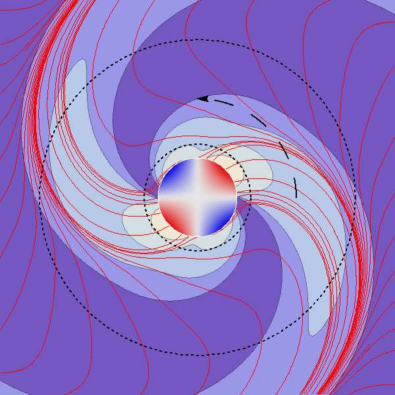
Figure 2: (color online). Some vortex lines (solid, red lines) and contours of vorticity (shaded regions) in the equatorial plane for the $(2,2)$ magnetic-parity quasinormal mode of a non-rotating, Schwarzschild black hole, with complex eigenfrequency $\omega=(0.37367-0.08896i)/M$ where $M$ is the hole’s mass. The horizon (central circle) is color coded by the horizon vorticity $\mathcal{B}_{NN}$ as seen by someone looking down on the black hole; this vorticity is entirely perturbative. The thick, solid red curves are one set of vortex lines in the equatorial plane—the set with negative vorticity. These lines include some that emerge from the horizon in the negative-vorticity (red) regions, and some that never reach the horizon. The other, positive-vorticity, equatorial vortex lines are orthogonal to the ones shown, and are identical to those shown but rotated through 90 degrees around the hole so some of them emerge from the horizon in the positive-vorticity (blue) regions. The contours represent the vorticity of the red (negative-vorticity) vortex lines, with largest magnitude of vorticity white and smallest purple (dark gray); the contours mark where the vorticity has fallen to $50\%$, $25\%$, $10\%$, and $5\%$ of the maximum value attained at the center of the horizon vortex. The two dotted circles are drawn at Schwarzschild radii $r=\lambdabar$ and $r=\pi\lambdabar=\lambda/2$. They mark the approximate outer edge of the near zone and the approximate inner edge of the wave zone. The arrow marks the direction of rotation of the perturbation.

We begin with the $(2,2)$ magnetic-parity mode of a Schwarzschild black hole. Figure 2 depicts the negative-vorticity vortex lines (red) and contours of their vorticity (white and purple [dark gray]), in the hole’s equatorial plane. Orthogonal to the red (solid) vortex lines (but not shown) are positive-vorticity, vortex lines that also lie in the equatorial plane. Vortex lines of the third family pass orthogonally through the equatorial plane. The entire configuration rotates counterclockwise, as indicated by the thick dashed arrow. The dotted lines, at radii $r=\lambdabar$ and $r=\pi\lambdabar$ (where $\lambdabar$ is the emitted waves’ reduced wavelength), mark the approximate outer edge of the near zone, and the approximate inner edge of the wave zone.

Just as the near-zone electromagnetic (1,1) perturbations are dominated by radial field lines that thread the black hole and have a dipolar distribution of field strength, so here the near-zone gravitational perturbations are dominated by (i) the radial vortex lines that thread the hole and have a quadrupolar distribution of their horizon vorticity $\mathcal{B}_{NN}=\delta\mathcal{B}_{NN}$, and also by (ii) a transverse, isotropic frame-drag field $\mathcal{B}_{\hat{\theta}\hat{\theta}}=\mathcal{B}_{\hat{\phi}\hat{\phi}}=-\frac{1}{2}\delta\mathcal{B}_{NN}$ that is tied to $\mathcal{B}_{NN}$ in such a way as to guarantee that this dominant part of $\bm{\mathcal{B}}$ is traceless.

This full structure, the normal-normal field and its accompanying isotropic transverse field, makes up the longitudinal, nonradiative frame-drag field ${\bm{\mathcal{B}}}^{\rm L}$ near the horizon. (As we shall discuss below, this longitudinal structure is responsible for generating the mode’s gravitational waves, and all of the rest of its fields.) Somewhat smaller are (i) the longitudinal-transverse components of $\bm{\mathcal{B}}$ ($\mathcal{B}_{\hat{r}\hat{\theta}}$ and $\mathcal{B}_{\hat{r}\hat{\phi}}$), which together make up the longitudinal-transverse part of the frame-drag field, a 2-vector ${\bm{\mathcal{B}}}^{\rm LT}$ parallel to the horizon, and give the horizon-piercing vortex lines small non-normal components; and (ii) transverse-traceless components $\mathcal{B}_{\hat{\theta}\hat{\theta}}=-\mathcal{B}_{\hat{\phi}\hat{\phi}}$, which make up the transverse-traceless part of the frame-drag field, a 2-tensor ${\bm{\mathcal{B}}}^{\rm TT}$ parallel to the horizon, and are ingoing gravitational waves as seen by Schwarzschild observers. (This decomposition into L, LT, and TT parts is useful only near the horizon and in the wave zone, where there are preferred longitudinal directions associated with wave propagation.)

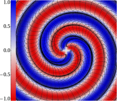
Figure 3: (color online). The vortex lines (solid black for clockwise; dashed black for counterclockwise) and color-coded vorticities in the equatorial plane for the same magnetic-parity $(2,2)$ mode as in Fig. 2. This figure differs from Fig. 2 in ways designed to give information about the emitted gravitational waves: (i) It extends rather far out into the wave zone. (ii) It shows the angular structure of the vorticity for the dominant vortex lines in each region of the equatorial plane. More specifically: the color at each point represents the vorticity of the equatorial vortex line there which has the largest magnitude of vorticity, with radial variations of vorticity normalized away (so the linear color code on the left indicates vorticity relative to the maximum at any given radius). The regions of large positive vorticity (blue [dark gray]) are clockwise vortexes; those of large negative vorticity (red [light gray]) are counterclockwise vortexes.

As the near-zone, longitudinal frame-drag field $\bm{\mathcal{B}}^{\rm L}$ rotates, it generates a near-zone longitudinal-transverse (LT) perturbative frame-drag field $\bm{\mathcal{B}}^{\rm LT}$ via $\bm{\mathcal{B}}$’s propagation equation (the wave equation for the Riemann tensor), and it generates a LT tidal field $\delta\bm{\mathcal{E}}^{\rm LT}$ via the Maxwell-like Bianchi identity which says, in a local Lorentz frame (for simplicity), $\partial\bm{\mathcal{E}}/\partial t=(\bm{\nabla}\times\bm{\mathcal{B}})^{\rm S}$, where the superscript S means “symmetrize” [Eq. (2.15) of Paper I]. These three fields, $\bm{\mathcal{B}}^{\rm L}$, $\bm{\mathcal{B}}^{\rm LT}$, and $\delta\bm{\mathcal{E}}^{\rm LT}$ together maintain each other during the rotation via this Maxwell-like Bianchi identity and its (local-Lorentz-frame) dual $\partial\bm{\mathcal{B}}/\partial t=-(\bm{\nabla}\times\bm{\mathcal{E}})^{\rm S}$. They also generate the transverse-traceless parts of both fields, $\bm{\mathcal{B}}^{\rm TT}$, and $\delta\bm{\mathcal{E}}^{\rm TT}$, which become the outgoing gravitational waves in the wave zone and ingoing gravitational waves at the horizon.

In the equatorial plane, this outgoing-wave generation process, described in terms of vortex and tendex structures, is quite pretty, and is analogous to the (1,1) magnetic-field mode of Fig. 1 and Sec. I.3.4: As one moves outward into the induction zone and then the wave zone, the equatorial vortex lines bend backward into outgoing spirals (Fig. 2) and gradually acquire accompanying tendex lines. The result, locally, in the wave zone, is the standard pattern of transverse, orthogonal red and blue vortex lines; and (turned by 45 degrees to them) transverse, orthogonal red and blue tendex lines, that together represent plane gravitational waves (Fig. 7 of Paper I).

It is instructive to focus attention on regions of space with large magnitude of vorticity. We call these regions vortexes. Figure 3 shows that the equatorial frame-drag field consists of four outspiraling vortexes, two red ([light gray] counterclockwise) and two blue ([dark gray] clockwise).

The solid black lines in the figure are clockwise vortex lines. In the clockwise vortexes of the wave zone, they have the large magnitude of vorticity that is depicted as blue (dark gray), and they are nearly transverse to the radial wave-propagation direction; so they represent crests of outgoing waves. In the counterclockwise vortexes (red [light gray] regions), these clockwise vortex lines have very small magnitude of vorticity and are traveling roughly radially, leaping through a red vortex (a wave trough) from one blue vortex (wave crest) to the next. These clockwise vortex lines accumulate at the outer edges of the clockwise (blue) vortexes.

Figure 4: (color online). Some 3-dimensional clockwise vortex lines (shown black) and regions of large vorticity (vortexes, shown blue [dark gray] and red [light gray]) and small vorticity (shown off-white), for the same magnetic-parity mode of a Schwarzschild black hole as in Figs. 2 and 3. More specifically: the inner sphere is the horizon, color coded by its vorticity. The blue region is a clockwise vortex in which one vortex line has vorticity at least 85% of the maximum value at that radius, and similarly for the counterclockwise red region. The four off-white regions are locations where no vortex line has magnitude of vorticity in excess of 25% of the maximum at that radius.

The dashed black lines are counterclockwise vortex lines, which are related to the red (light gray), counterclockwise vortexes in the same way as the solid clockwise vortex lines are related to the blue (dark gray), clockwise vortexes.

Outside the equatorial plane, this mode also represents outgoing gravitational waves, once one gets into the wave zone. We depict the strengths of the vortexes which become those waves in Fig. 4. The blue (dark gray) regions are locations where one vortex line has vorticity at least 85% of the maximum at that radius; in this sense, they are clockwise vortexes. In the near zone, two (blue) clockwise vortexes emerge radially from the horizon parallel to the plane of the picture, and two (red) counterclockwise vortexes emerge radially toward and away from us. These are 3-dimensional versions of the four vortexes emerging from the horizon in the equatorial plane of Fig. 3. In the wave zone, the “85%” vortexes are concentrated in the polar regions, because this mode emits its gravitational waves predominantly along the poles. The waves are somewhat weaker in the equatorial plane, so although there are spiraling vortexes in and near that plane (Fig. 3), they do not show up at the 85% level of Fig. 4. The off-white, spiral-arm structures in the equatorial plane represent the four regions where the wave strength is passing through a minimum.

Turn attention from the wave zone to the horizon. There the ingoing waves, embodied in ${\bm{\mathcal{B}}}^{\rm TT}$ and $\delta{\bm{\mathcal{E}}}^{\rm TT}$ (which were generated in the near and transition zones by rotation of $\bm{\mathcal{B}}^{\rm L}$), act back on $\bm{\mathcal{B}}^{\rm L}$, causing its vortex lines to gradually slide off the horizon and thereby producing the mode’s exponential decay.

Just as this process in the electromagnetic case is associated with the differential conservation law (3) for magnetic field lines threading the horizon, $\partial B_{N}/\partial t+{{}^{(2)}\bm{\nabla}\cdot(\alpha\bm{B}^{\rm T})}$, so also here it is associated with an analogous (approximate) conservation law and an accompanying driving equation, given in terms of two Newman Penrose equations (112) of Appendix E and the perturbative parts of the Weyl scalars $\Psi_{0}$, $\Psi_{1}$, and $\Psi^{(0)}_{2}$ :

$${\bf D}\Psi_{2}^{(1)}=({\bm{\delta}}^{*}+2\pi-2\alpha)\Psi_{1}\,,$$ (4a)

$$({\bf D}-2\epsilon)\Psi_{1}=({\bm{\delta}}^{*}+\pi-4\alpha)\Psi_{0}\,.$$ (4b)

(Note that only $\Psi_{2}$ is nonzero for the background spacetime with our tetrad choice.) Here the notation is that of Newman and Penrose: $\bf D$ is a time derivative on the horizon, $\Psi_{2}^{(1)}$ is the mode’s $\delta{\bm{\mathcal{E}}}^{\rm L}+i{\bm{\mathcal{B}}}^{\rm L}$ (equivalently $\delta\mathcal{E}_{NN}+i\mathcal{B}_{NN}$ in disguise), with $\delta{\bm{\mathcal{E}}}^{\rm L}$ and $\delta\mathcal{E}_{NN}$ vanishing for our mode; $\Psi_{1}$ is the LT field $\delta{\bm{\mathcal{E}}}^{\rm LT}+i\delta{\bm{\mathcal{B}}}^{\rm LT}$ (as measured by Schwarzschild observers) in disguise; $\Psi_{0}$ is the ingoing-wave $\delta{\bm{\mathcal{E}}}^{\rm TT}+i\delta{\bm{\mathcal{B}}}^{\rm TT}$ (as measured by Schwarzschild observers) in disguise; ${\bm{\delta}}^{*}$ is a divergence in disguise; and $\epsilon$, $\pi$ and $\alpha$ are NP spin coefficients. Equation (4b) says that the ingoing waves embodied in $\delta{\bm{\mathcal{E}}}^{\rm TT}+i{\bm{\mathcal{B}}}^{\rm TT}$ drive the evolution of the quantity $\Psi_{1}$, and Equation (4a) is an approximate differential conservation law in which this $\Psi_{1}$ plays the role of the flux of longitudinal vortex lines (number crossing a unit length per unit time) and $\Psi_{2}$ (i.e., $\mathcal{B}_{NN}$) is the density of longitudinal vortex lines. This differential conservation law says that the time derivative of the vortex-line density plus the divergence of the vortex-line flux is equal to some spin-coefficient terms that, we believe, are generally small. (By integrating this approximate conservation law over the horizon $\mathcal{H}$, we see that $\int_{\mathcal{H}}B_{NN}dA$ must be nearly conserved, in accord with Eq. (2) above, which tells us that the horizon integral is nearly zero. In both cases, the integral conservation law (2) and the differential conservation law (4a), it is numerically small spin coefficients that slightly spoil the conservation for vacuum perturbations of black holes. In Eq. (28), for a magnetic-parity mode of Schwarzschild and Eddington-Finkelstein slicing, we make this conservation law completely concrete and find that in this case it is precise; there are no small spin coefficients to spoil it. We plan to investigate this conservation law in numerical simulations as well, in which there may be additional subtleties related to the formation of caustics.

Returning to the evolution of the (2,2) magnetic-parity mode: The ingoing waves, via Eqs. (4), push the longitudinal vortex lines away from the centers of the horizon vortexes toward their edges (toward the white horizon regions in Figs. 2 and 3. At the edges, clockwise vortex lines from the blue (dark gray) horizon vortex and counterclockwise from the red (light gray) horizon vortex meet and annihilate each other, leading to decay of the longitudinal part of the field and thence the entire mode.

We expect to explore this evolutionary process in greater detail and with greater precision in future work.

Turn, next, to spinning black holes. In this case, the $(2,2)$ magnetic-parity mode has qualitatively the same character as for a non-spinning black hole. The principal change is due to the spin raising the mode’s eigenfrequency, and the near zone thereby essentially disappearing, so the perturbed vortex lines that emerge from the horizon have a significant back-spiral-induced tilt to them already at the horizon. See Fig. 12 below.

I.3.7 The (2,1) magnetic-parity mode of a Schwarzschild hole

For the (2,1) magnetic-parity mode of a Schwarzschild black hole, there are two horizon vortexes in the hole’s northern hemisphere (one counterlockwise, the other clockwise), and two in the southern hemisphere. From these emerge the longitudinal part of the frame-drag field, in the form of four 3D vortexes (Fig. 5).

Figure 5: (color online). Three-dimensional vortexes for the magnetic-parity, (2,1) mode of a Schwarzschild black hole. The colored surfaces enclose the region where, for each radius, the vorticity of at least one vortex line exceeds 90% of the maximum for that radius. In the blue and red (dark and light gray) regions, the clockwise and counterclockwise vortex lines, respectively, have the larger vorticity.

These four vortexes actually form two spiral arms, each of which contains vortex lines of both signs (clockwise and counterclockwise). The surface of each arm is color coded by the sign of the vorticity that is largest in magnitude in that region of the arm. This dominant vorticity flips sign when one passes through the equatorial plane—from positive (i.e., blue [dark gray]; clockwise) on one side of the equator to negative (i.e., red [light gray]; clockwise) on the other side. The reason for this switch is that for $m=1$ the $e^{im\phi}$ angular dependence means reflection antisymmetry through the polar axis, which combined with the positive parity of the $l=2$ frame-drag field implies reflection antisymmetry through the equatorial plane. The (2,2) mode of the previous section, by contrast, was reflection symmetric through both the polar axis and the equatorial plane.

By contrast with the (2,2) mode, whose region of largest vorticity switched from equatorial in the near zone to polar in the wave zone (Fig. 3), for this (2,1) mode, the region of largest vorticity remains equatorial in the wave zone. In other words, this mode’s gravitational waves are stronger in near-equator directions than in near-polar directions. (Recall that in the wave zone, the vortexes are accompanied by tendexes with tendicities equal in magnitude to the vorticities at each event, so we can discuss the gravitational-wave strengths without examining the tidal field.)

Close scrutiny of the near-horizon region of Fig. 5 reveals a surprising feature: Within the 90% vortexes (colored surfaces), the sign of the largest vorticity switches as one moves from the near zone into the transition zone—which occurs not very far from the horizon; see the inner dashed circle in Fig. 2 above). This appears to be due to the following: The near-zone vortexes are dominated by the longitudinal part of the frame-drag field $\delta{\mathcal{B}}^{\rm L}$, which generates all the other fields including $\delta{\bm{\mathcal{B}}}^{\rm LT}$ via its rotation [see discussion of the (2,2) mode above]. The longitudinal-transverse field $\delta{\bm{\mathcal{B}}}^{\rm LT}$ is strong throughout the near zone and comes to dominate over $\delta{\bm{\mathcal{B}}}^{\rm L}$ as one moves into the transition zone. Its largest vorticity has opposite sign from that of $\delta{\bm{\mathcal{B}}}^{\rm L}$, causing the flip of the dominant vorticity and thence the color switch as one moves into the transition zone. (Note that a similar switch in the sign of the strongest vorticity occurs for the magnetic-parity (2,2) mode vortexes illustrated in Fig. 4, although there the transition occurs farther out, at the edge of the wave zone.)

In Secs. V.1 and V.2, we explore in considerable detail this magnetic-parity (2,1) mode and also its near dual, the electric-parity (2,1) mode, focusing especially on the shapes of their vortexes.

I.3.8 The (2,0) magnetic-parity mode of a Schwarzschild hole

The (2,0) magnetic-parity mode has very different dynamical behavior from that of the (2,1) and (2,2) modes. Because of its axisymmetry, this mode cannot be generated by longitudinal, near-zone vortexes that rotate around the polar axis, and its waves cannot consist of outspiraling, intertwined vortex and tendex lines.

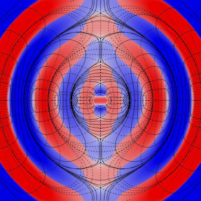
Figure 6: (color online). Vortex lines and vorticities for magnetic-parity (2,0) mode of Schwarzschild in a surface $\mathcal{S}_{\phi}$ of constant $\phi$. The line and coloring conventions are the same as in Fig. 3 (solid lines for clockwise, dashed for counterclockwise; color shows vorticity of the vortex line with largest magnitude of vorticity, with radial variations removed and intensity of color as in the key on right edge of Fig. 3). The central circle is the horizon, color coded by the horizon vorticity.

Instead, this mode is generated by longitudinal, near-zone vortexes that oscillate, and its waves are made up of intertwined vortex lines and tendex lines that wrap around deformed tori. These gravitational-wave tori resemble smoke rings and travel outward at the speed of light. More specifically:

Because of axisymmetry, the (2,0) magnetic-parity mode has one family of vortex lines that are azimuthal circles of constant $r$ and $\theta$, and two families that lie in surfaces $\mathcal{S}_{\phi}$ of constant $\phi$. Figure 6 is a plot in one of these $\mathcal{S}_{\phi}$ surfaces. (The plot for any other $\phi$ will be identical to this, by axisymmetry.) This plot shows the vortex lines that lie in $\mathcal{S}_{\phi}$, and by color coding at each point, the vorticity of the strongest of those lines.

Notice that, at this phase of oscillation, there are clockwise (solid) vortex lines sticking nearly radially out of the horizon’s polar regions and counterclockwise (dashed) vortex lines sticking nearly radially out of the horizon’s equatorial region. A half cycle later the poles will be red (light gray) and equator blue (dark gray). These near-zone vortex lines are predominantly the longitudinal part of the frame-drag field $\delta{\bm{\mathcal{B}}}^{\rm L}$, which we can regard as working hand in hand with the near-zone, longitudinal-transverse tidal field $\delta{\bm{\mathcal{E}}}^{\rm LT}$ to generate the other fields.

As we shall see in Sec. V.3 (and in more convincing detail for a different oscillatory mode in Sec. IV.3), the dynamics of the oscillations are these: Near-zone energy oscillates back and forth between the near-zone $\delta{\bm{\mathcal{B}}}^{\rm L}$, and the near-zone $\delta{\bm{\mathcal{B}}}^{\rm LT}$ and $\delta{\bm{\mathcal{E}}}^{\rm LT}$. As $\delta{\bm{\mathcal{B}}}^{\rm L}$ decays, its vortex lines slide off the hole and (we presume) form closed loops, lying in $\mathcal{S}_{\phi}$, which encircle outgoing deformed tori of perturbed tendex lines that become the transverse-traceless gravitational waves. Only part of the energy in $\delta{\bm{\mathcal{B}}}^{\rm L}$ goes into the outgoing waves. Some goes into the TT ingoing waves, and the rest (a substantial fraction of the total energy) goes into $\delta{\bm{\mathcal{B}}}^{\rm LT}$ and $\delta{\bm{\mathcal{E}}}^{\rm LT}$, which then use it to regenerate $\delta{\bm{\mathcal{B}}}^{\rm L}$, with its horizon-penetrating vortex lines switched in sign (color), leading to the next half cycle of oscillation.

The vortex lines that encircle the gravitational-wave tori are clearly visible in Fig. 6. Each solid (clockwise) line is tangential (it points nearly in the $\theta$ direction) when it is near the crest (the maximum-vorticity surface) of a blue (dark gray), lens-shaped gravitational-wave vortex. As it nears the north or south pole, it swings radially outward becoming very weak (low vorticity) and travels across the red trough of the wave, until it nears the next blue crest. There it swings into the transverse, $\theta$ direction and travels toward the other pole, near which it swings back through the red trough and joins onto itself in the original blue crest.

Each dashed (counterclockwise) closed vortex line behaves in this same manner, but with its transverse portions lying near red (light gray) troughs (surfaces of most negative vorticity). Near the red troughs, there are blue azimuthal vortex lines (not shown) that encircle the hole in the $\phi$ direction, and near the blue crests, there are red azimuthal lines.

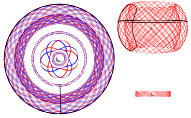
Figure 7: (color online). Positive-tendicity (blue) and negative-tendicity (red) perturbative tendex lines of a $(2,0)$ magnetic-parity perturbation of a Schwarzschild black hole. These lines spiral around deformed tori of progressively larger diameter. The viewpoint is looking down onto the equatorial plane from the positive symmetry axis. Upper right inset: The negative tendex line spiraling around the outermost torus, viewed in cross section from the equatorial plane. Lower right inset: The negative tendex line spiraling around the small torus third from the center, viewed in cross section from the equatorial plane. Also shown, in black in the main drawing and the large inset, are two of this mode’s vortex lines, one from Fig. 6 wrapping around the outermost torus in a $\mathcal{S}_{\phi}$ plane; the other an azimuthal circle wrapping around that torus in the $\phi$ direction. This figure was actually drawn depicting vortex lines of the electric-parity mode discussed in Sec. V.4; but by duality (which is excellent in the wave zone), it also represents the tendexes of the magnetic-parity mode discussed in this section.

Figure 7 sheds further light on these gravitational-wave tori. It shows in three dimensions some of the perturbative tendex lines for the (2,0) magnetic-parity mode that we are discussing. (For this mode, two families of perturbative tendex lines, one red [counterclockwise] and the other blue [clockwise], have nonzero tendicity and the third family has vanishing tendicity.) As is required by the structure of a gravitational wave (transverse tendex lines rotated by 45 degrees relative to transverse vortex lines), these perturbative tendex lines wind around tori with pitch angles of 45 degrees; one family winds clockwise and the other counterclockwise, and at each point the two lines have the same magnitude of vorticity.

A close examination of Fig. 7 reveals that the tori around which the perturbative tendex lines wrap are half as thick as the tori around which the vortex lines wrap. Each tendex-line torus in Fig. 7 is centered on a single node of the gravitational-wave field; the thick red torus in the upper right panel reaches roughly from one crest of the wave to an adjacent trough. By contrast, each vortex-line torus (Fig. 6 and black poloidal curves in Fig. 7) reach from crest to crest or trough to trough and thus encompass two gravitational-wave nodes.

Each node in the wave zone has a family of nested tendex-line tori centered on it. The four tendex-line tori shown in Fig. 7 are taken from four successive families, centered on four successive nodes. The second thin torus is from near the center of one nested family; it tightly hugs a node and therefore has near vanishing tendicity. The two thick tori are from the outer reaches of their nested families.

For further details of the (2,0) modes, see Secs. V.3 and V.4 below.

I.3.9 The superposed $(2,2)$ and $(2,-2)$ magnetic-parity mode of a Schwarzschild hole

As we have seen, the magnetic-parity, $(2,2)$ mode of a Schwarzschild black hole represents vortexes that rotate counterclockwise around the hole, spiraling outward and backward (Figs. 2, 3 and 4 above). If we change the sign of the azimuthal quantum number to $m=-2$, the vortexes rotate in the opposite direction, and spiral in the opposite direction. If we superpose these two modes (which, for Schwarzschild, have the same eigenfrequency), then, naturally, we get a non-rotating, oscillatory mode—whose dynamics are similar to those of the (2,0) mode of the last subsection. See Sec. IV for details.

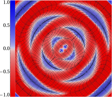
Figure 8: (color online). Equatorial vortex structure of the superposed $(2,2)$ and $(2,-2)$, magnetic-parity, fundamental modes of a Schwarzschild black hole. The colors encode the vorticity of the dashed vortex lines. The vorticity of the solid lines is not shown, but can be inferred from the fact that under a $90^{\circ}$ rotation, the dashed lines map into solid and the solid into dashed.

Figure 8 is a snapshot of the two families of vortex lines that lie in this mode’s equatorial plane. The plane is colored by the vorticity of the dashed vortex lines; they are predominantly counterclockwise (red), though in some regions they are clockwise (blue).

The red (light gray) regions form interleaved rings around the black hole, that expand outward at the speed of light, along with their dashed vortex lines. These rings are not tori in three dimensions because [by contrast with the $(2,0)$ mode] the frame drag field grows stronger as one moves up to the polar regions, rather than weakening. As the mode oscillates, the longitudinal near-zone frame-drag field $\bm{\mathcal{B}}^{\rm L}$, which drives the mode, generates new interleaved rings, one after another and sends them outward.

During the oscillations, there are phases at which the longitudinal field $\bm{\mathcal{B}}^{\rm L}$ threading the hole goes to zero, and so the hole has vanishing horizon vorticity. The near-zone oscillation energy, at these phases, is locked up in the near-zone, longitudinal-transverse fields $\bm{\mathcal{B}}^{\rm LT}$ and $\delta\bm{\mathcal{E}}^{\rm LT}$, which, via the Maxwell-like Bianchi identities (and the propagation equation that they imply), then feed energy into the longitudinal near-zone frame-drag field $\bm{\mathcal{B}}^{\rm L}$, thereby generating new horizon-threading vortex lines, which will give rise to the next ejected interleaved ring.

We explore these dynamics in greater detail in Sec. IV.3.

I.4 This paper’s organization

The remainder of this paper is organized as follows: In Sec. II, we introduce the time slicing and coordinates used throughout this paper for the background Schwarzschild and Kerr spacetimes, we introduce the two gauges that we use for Schwarzschild perturbations (Regge-Wheeler-Zerilli and ingoing radiation gauges) and the one gauge (ingoing radiation) we use for Kerr, we discuss how our various results are affected by changes of gauge, and we discuss how we perform our computations. In Secs. III, IV, and V, we present full details of our results for the fundamental (most slowly damped) quadrupolar modes of Schwarzschild and Kerr: (2,2) modes in Sec. III; superposed (2,2) and (2,-2) modes in Sec. IV, and both (2,1) and (2,0) modes in Sec. V. In Sec. III.4, we compare vortex lines computed in a numerical-relativity simulation of a binary black hole at a late time, when the merged hole is ringing down, with the vortex lines from this paper for the relevant quasinormal mode; we obtain good agreement. In Sec. VI, we make a few concluding remarks. And in six appendices, we present mathematical details that underlie a number of this paper’s computations and results.

II Slicings, Gauges and Computational Methods

When calculating the tidal and frame-drag fields of perturbed black-hole spacetimes, we must choose a slicing and also spatial coordinates on each slice, for both the background spacetime and at first order in the perturbations (“perturbative order”). The perturbative-order choices of slicing and spatial coordinates are together called the chosen gauge. We will always use the same choice of background slicing and coordinates in this study, but we will use different choices for our gauge.

This section describes the choices we make, how they influence the vortex and tendex lines and their vorticities and tendicities (which together we call the “vortex and tendex structures”), and a few details of how, having made our choices, we compute the perturbative frame-drag and tidal fields and the vortex and tendex structures. Most of the mathematical details are left to later sections and especially appendices.

In Sec. II.1, we describe our choices of slicing and spatial coordinates. In Sec. II.2, we sketch how we calculate the perturbative frame-drag and tidal fields and visualize their vortex and tendex structures. In Sec. II.3, we explore how those structures change under changes of gauge, i.e., changes of the perturbative slicing and perturbative spatial coordinates.

II.1 Slicing, spatial coordinates, and gauge

Throughout this paper, for the background (unperturbed) Kerr spacetime, we use slices of constant Kerr-Schild (KS) time $\tilde{t}$, which is related to the more familiar Boyer-Lindquist time by

$$\tilde{t}=t+r_{*}-r\;,\quad{\rm where}\quad{dr_{*}\over dr}={r^{2}+a^{2}\over\Delta}\;$$ (5)

(Eq. (6.2) of Paper II Zhang et al. (2012)). Here $t$ and $r$ are the Boyer-Lindquist time and radial coordinates, $a$ is the black hole’s spin parameter (angular momentum per unit mass), and $\Delta\equiv r^{2}-2Mr+a^{2}$, with $M$ the black-hole mass. Our slices of constant $\tilde{t}$ penetrate the horizon smoothly, by contrast with slices of constant $t$, which are singular at the horizon. In the Schwarzschild limit $a\rightarrow 0$, $t$ and $r$ become Schwarzschild’s time and radial coordinates, and $\tilde{t}$ becomes ingoing Eddington-Finkelstein time, $\tilde{t}=t+2M\ln|r/2M-1|$.

On a constant-$\tilde{t}$ slice in the background Kerr spacetime, we use Cartesian-like KS (Kerr-Schild) spatial coordinates, when visualizing vortex and tendex structures; but in many of our intermediary computations, we use Boyer-Lindquist spatial coordinates $\{r,\theta,\phi\}$ (which become Schwarzschild as $a\rightarrow 0$). The two sets of coordinates are related by

$$x+iy=(r+ia)e^{i\tilde{\phi}}\sin\theta\;,\quad z=r\cos\theta\;,$$ (6)

[Eq. (6.7) of Paper II]. Here

$$\tilde{\phi}=\phi+\int_{r}^{\infty}{a\over\Delta}dr$$ (7)

[Eq. (6.5) of Paper II] is an angular coordinate that, unlike $\phi$, is well behaved at the horizon. In the Schwarzschild limit, the KS $\{x,y,z\}$ coordinates become the quasi-Cartesian $\{x,y,z\}$ associated with Eddington-Finkelstein (EF) spherical coordinates $\{r,\theta,\phi\}$.

Our figures (e.g., 2–8 above) are drawn as though the KS $\{x,y,z\}$ were Cartesian coordinates in flat spacetime—i.e., in the Schwarzschild limit, as though the EF $\{r,\theta,\phi\}$ were spherical polar coordinates in flat spacetime.

We denote by $g^{(0)}_{\mu\nu}$ the background metric in KS spacetime coordinates [Eq. (6.8) of Paper II] (or EF spacetime coordinates in the Schwarzschild limit). When the black hole is perturbed, the metric acquires a perturbation $h_{\mu\nu}$ whose actual form depends on one’s choice of gauge—i.e., one’s choice of slicing and spatial coordinates at perturbative order.

For Schwarzschild black holes, we use two different gauges, as a way to assess the gauge dependence of our results: (i) Regge-Wheeler-Zerilli (RWZ) gauge, in which $h_{\mu\nu}$ is a function of two scalars ($Q$ for magnetic parity and $Z$ for electric parity) that obey separable wave equations in the Schwarzschild spacetime and that have spin-weight zero (see App. A for a review of this formalism), and (ii) ingoing radiation (IR) gauge, in which $h_{\mu\nu}$ is computed from the Weyl scalar $\Psi_{0}$ (or $\Psi_{4}$) that obeys the separable Bardeen-Press equation. The method used to compute the metric perturbation from $\Psi_{0}$ is often called the Chrzanowski-Cohen-Kegeles (CCK) procedure of metric reconstruction (see App. C).

In App. D, we exhibit explicitly the relationship between the RWZ and IR gauges, for electric- and magnetic-parity perturbations. The magnetic-parity perturbations have different perturbative spatial coordinates, but the same slicing. (In fact, all gauges related by a magnetic-parity gauge transform have identically the same slicing for magnetic-parity perturbations of Schwarzschild [although the same is not true for Kerr]; see Sec. II.3). For electric-parity perturbations, the two gauges have different slicings and spatial coordinates.

For all the perturbations that we visualize in this paper, the tendexes and vortexes show quite weak gauge dependence. See, e.g., Sec. III, where we present results from both gauges. The results in Secs. IV and V are all computed in RWZ gauge.

For Kerr black holes, there is no gauge analogous to RWZ; but the IR gauge and the CCK procedure that underlies it are readily extended from Schwarzschild to Kerr. In this extension, one constructs the metric perturbation from solutions to the Teukolsky equation (see App. B) for the perturbations to the Weyl scalars $\Psi_{0}$ and $\Psi_{4}$, in an identical way to that for a Schwarzschild black hole described above. Our results in this paper for Kerr black holes, therefore, come solely from the IR gauge.

II.2 Sketch of computational methods

This section describes a few important aspects of how we calculate the tidal and frame-drag fields, and their vortex and tendex structures which are visualized and discussed in Secs. III, IV, and V.

We find it convenient to solve the eigenvalue problem in an orthonormal basis (orthonormal tetrad) given by the four-velocities of the Kerr-Schild (KS) or Eddington-Finkelstein (EF) observers, and a spatial triad, $\vec{e}_{\hat{a}}$, carried by these observers.

The background EF tetrad for the Schwarzschild spacetime, expressed in terms of Schwarzschild coordinates, is

$$\vec{u}^{\,(0)} = \frac{1}{\sqrt{1+2M/r}}\left(\frac{1}{\alpha^{2}}\frac{\partial}{\partial t}-\frac{2M}{r}\frac{\partial}{\partial r}\right)\;,$$

$$\vec{e}^{\,(0)}_{\hat{r}} = \frac{1}{\sqrt{1+2M/r}}\left(\frac{\partial}{\partial r}-\frac{2M}{\alpha^{2}r}\frac{\partial}{\partial t}\right)\;,$$

$$\vec{e}^{\,(0)}_{\hat{\theta}} = \frac{1}{r}\frac{\partial}{\partial\theta}\;,\qquad\vec{e}^{\,(0)}_{\hat{\phi}}=\frac{1}{r\sin\theta}\frac{\partial}{\partial\phi}\;$$ (8)

[cf. Eqs. (4.4) of Paper II, which, however, are written in terms of the EF coordinate basis rather than Schwarzschild]. The background orthonormal tetrad for KS observers (in ingoing Kerr coordinates $\{\tilde{t},r,\theta,\tilde{\phi}\}$; see Paper II, Sec. VI C) is

$$\vec{u}^{\,(0)} =H\partial_{\tilde{t}}-\frac{2Mr}{H\Sigma}\partial_{r}\,, \vec{e}^{\,(0)}_{\hat{r}} =\frac{\sqrt{A}}{H\Sigma}\partial_{r}+\frac{aH}{\sqrt{A}}\partial_{\tilde{\phi}}\,,$$

$$\vec{e}^{\,(0)}_{\hat{\theta}} =\frac{1}{\sqrt{\Sigma}}\partial_{\theta}\,, \vec{e}^{\,(0)}_{\hat{\tilde{\phi}}} =\sqrt{\frac{\Sigma}{A}}\frac{1}{\sin\theta}\partial_{\tilde{\phi}}\,,$$ (9a)

where we have defined

$$\Sigma =r^{2}+a^{2}\cos^{2}\theta\,,$$ (9b)

$$H =1+\frac{2Mr}{\Sigma}\,,$$ (9c)

$$A =(r^{2}+a^{2})^{2}-a^{2}(r^{2}-2Mr+a^{2})\sin^{2}\theta\,$$ (9d)

[see Eq. (B2) of Paper II].

When the black hole is perturbed, the tetrad $\{\vec{u}^{(0)},\vec{e}_{\hat{r}}^{\,(0)},\vec{e}_{\hat{\theta}}^{\,(0)},\vec{e}_{\hat{\tilde{\phi}}}^{\,(0)}\}$ acquires perturbative corrections that keep it orthonormal with respect to the metric $g_{\mu\nu}=g^{(0)}_{\mu\nu}+h_{\mu\nu}$. We choose the perturbative corrections to the observers’ 4-velocity so as to keep it orthogonal to the space slices, i.e., so as to keep $\vec{u}=-\alpha\vec{\nabla}\tilde{t}$. (Here $\alpha=d\tau/d\tilde{t}$, differentiating along the observer’s world line, is the observer’s lapse function.) A straightforward calculation using the perturbed metric gives the following contravariant components of this $\vec{u}$:

$$u^{\mu} =u^{\mu}_{(0)}+u^{\mu}_{(1)}\,,$$

$$u^{\mu}_{(1)} =-\frac{1}{2}h_{\hat{0}\hat{0}}u^{\mu}_{(0)}-h^{\mu\nu}u^{(0)}_{\nu}\,.$$ (10)

where $h_{\hat{0}\hat{0}}=h_{\mu\nu}u^{\mu}_{(0)}u^{\nu}_{(0)}$, and $u^{\mu}_{(0)}$ is the four-velocity of the background observers.

We choose the perturbative corrections to the spatial triad $\{\vec{e}_{\hat{j}}\}$ so the radial vector stays orthogonal to surfaces of constant $r$ in slices of constant $\tilde{t}$, the $\hat{\theta}$ direction continues to run orthogonal to curves of constant $\theta$ in surfaces of constant $r$ and $\tilde{t}$, and the $\hat{\phi}$ vector changes only in its normalization.

When written in terms of the unperturbed tetrad and projections of the metric perturbation into the unperturbed tetrad, the perturbation to the tetrad then takes the form

$$\vec{u}_{(1)} = \frac{1}{2}h_{\hat{0}\hat{0}}\vec{u}_{(0)}-h_{\hat{0}\hat{i}}\vec{e}_{(0)}^{\,\hat{i}}\,,$$ (11a)

$$\vec{e}_{\hat{r}}^{\,(1)} = -\frac{1}{2}h_{\hat{r}\hat{r}}\vec{e}_{\hat{r}}^{\,(0)}-h_{\hat{r}\hat{A}}\vec{e}_{(0)}^{\,\hat{A}}\,,$$ (11b)

$$\vec{e}_{\hat{\theta}}^{\,(1)} = -\frac{1}{2}h_{\hat{\theta}\hat{\theta}}\vec{e}_{\hat{\theta}}^{\,(0)}-h_{\hat{\theta}\hat{\phi}}\vec{e}_{(0)}^{\,\hat{\phi}}\,,$$ (11c)

$$\vec{e}_{\hat{\phi}}^{\,(1)} = -\frac{1}{2}h_{\hat{\phi}\hat{\phi}}\vec{e}_{\hat{\phi}}^{\,(0)}\,,$$ (11d)

where $\hat{i}$ is summed over $\hat{r}$, $\hat{\theta}$, and $\hat{\phi}$, and $\hat{A}$ is summed over only $\hat{\theta}$ and $\hat{\phi}$.

In Appendices A (RWZ gauge) and C (IR gauge), we give the details of how we compute the components

$$\mathcal{E}_{\hat{i}\hat{j}}=\mathcal{E}_{\hat{i}\hat{j}}^{(0)}+\mathcal{E}_{\hat{i}\hat{j}}^{(1)}\,,\quad\mathcal{B}_{\hat{i}\hat{j}}=\mathcal{B}_{\hat{i}\hat{j}}^{(0)}+\mathcal{B}_{\hat{i}\hat{j}}^{(1)}\,.$$ (12)

of the tidal and frame-drag field in this perturbed tetrad. The background portions $\mathcal{E}_{\hat{i}\hat{j}}^{(0)}$ and $\mathcal{B}_{\hat{i}\hat{j}}^{(0)}$ are the stationary fields of the unperturbed black hole, which were computed and visualized in Paper II. The perturbative pieces, $\mathcal{E}_{\hat{i}\hat{j}}^{(1)}$ and $\mathcal{B}_{\hat{i}\hat{j}}^{(1)}$ are the time-dependent, perturbative parts, which carry the information about the quasinormal modes, their geometrodynamics, and their gravitational radiation.

As part of computing the perturbative $\mathcal{E}_{\hat{i}\hat{j}}^{(1)}\equiv\delta\mathcal{E}_{\hat{i}\hat{j}}$ and $\mathcal{B}_{\hat{i}\hat{j}}^{(1)}\equiv\delta\mathcal{B}_{\hat{i}\hat{j}}$ for a chosen quasinormal mode of a Kerr black hole, we have to solve for the mode’s Weyl-scalar eigenfunctions $\Psi_{0}^{(1)}$ and $\Psi_{4}^{(1)}$ and eigenfrequency $\omega$. To compute the frequencies, we have used, throughout this paper, Emanuele Berti’s elegant computer code Ber , which is discussed in Berti et al. (2009) and is an implementation of Leaver’s method Leaver (1985). To compute the eigenfunctions, we our own independent code (which also uses the same procedure as that of Berti). In App. C, we describe how we extract the definite-parity (electric or magnetic) eigenfunctions from the non-definite-parity functions.

To best visualize each mode’s geometrodynamics and generation of gravitational waves in Secs. III, IV, and V, we usually plot the tendex and vortex structures of the perturbative fields $\mathcal{E}_{\hat{i}\hat{j}}^{(1)}$ and $\mathcal{B}_{\hat{i}\hat{j}}^{(1)}$. However, when we compare our results with numerical-relativity simulations, it is necessary to compute the tendex and vortex structures of the full tidal and frame-drag fields (background plus perturbation), because of the difficulty of unambiguously removing a stationary background field from the numerical simulations. As one can see in Figs. 15 and 26, in this case much of the detail of the geometrodynamics and wave generation is hidden behind the large background field.

In either case, the tendex and vortex structure of the perturbative fields or the full fields, we compute the field lines and their eigenvalues in the obvious way: At selected points on a slice, we numerically solve the eigenvalue problem

$$\mathcal{E}_{\hat{i}\hat{j}}V_{\hat{j}}=\lambda V_{\hat{i}}$$ (13)

for the three eigenvalues $\lambda$ and unit-normed eigenvectors $V_{\hat{i}}$ of $\mathcal{E}_{\hat{i}\hat{j}}$, and similarly for $\mathcal{B}_{\hat{i}\hat{j}}$; and we then compute the integral curve (tendex or vortex line) of each eigenvector field by evaluating its coordinate components $V^{j}$ in the desired coordinate system (KS or EF) and then numerically integrating the equation

$${dx^{j}\over ds}=V^{j}\;,$$ (14)

where $s$ is the proper distance along the integral curve.

II.3 Gauge changes: Their influence on tidal and frame-drag fields and field lines

For perturbations of black holes, a perturbative gauge change is a change of the spacetime coordinates, $x^{\alpha^{\prime}}=x^{\alpha}+\xi^{\alpha}$, that induces changes of the metric that are of order the metric perturbation; when dealing with definite parity perturbation, we split the generator of the transform $\xi^{\alpha}$ into definite electric- and magnetic-parity components. The gauge change has two parts: A change of slicing generated by $\xi^{0}$, and a change of spatial coordinates

$${\tilde{t}}^{\prime}=\tilde{t}+\xi^{0}\quad x^{j^{\prime}}=x^{j}+\xi^{j}\;.$$ (15)

Here all quantities are to be evaluated at the same event, $\mathcal{P}$, in spacetime.

Because $\xi^{0}$ is a scalar under rotations in the Schwarzschild spacetime—and all scalar fields in Schwarzschild have electric parity—for a magnetic-parity $\xi^{\alpha}$, $\xi^{0}$ vanishes, and the slicings for magnetic-parity quasinormal modes of Schwarzschild are unique. For these modes, all gauges share the same slicing (see Appendix D).

II.3.1 Influence of a perturbative slicing change

For (electric-parity) changes of slicing, the new observers, whose world lines are orthogonal to the new slices, $\tilde{t}^{\prime}=$const, move at velocity

$$\Delta\bm{v}=-\alpha\bm{\nabla}\xi^{0}$$ (16)

with respect to the old observers, whose world lines are orthogonal to the old slices $\tilde{t}=$const). Here $\bm{\nabla}$ is the gradient in the slice of constant $\tilde{t}$, and $\alpha=(d\tau/d\tilde{t})$ is the lapse function, evaluated along the observer’s worldline. In other words, $\Delta\bm{v}$ is the velocity of the boost that leads from an old observer’s local reference frame to a new observer’s local reference frame. Just as in electromagnetic theory, this boost produces a change in the observed electric and magnetic fields for small $\Delta\bm{v}$ given by $\Delta\bm{B}=\Delta\bm{v}\times\bm{E}$ and $\Delta\bm{E}=-\Delta\bm{v}\times\bm{B}$, so also it produces a change in the observed tidal and frame-drag fields given by

$$\Delta\bm{\mathcal{B}}=(\Delta\bm{v}\times\bm{\mathcal{E}})^{\rm S}\;,\quad\Delta\bm{\mathcal{E}}=-(\Delta\bm{v}\times\bm{\mathcal{B}})^{\rm S}\;$$ (17)

(e.g., Eqs. (A12) and (A13) of Maartens et al. (1999), expanded to linear order in the boost velocity). Here the superscript S means symmetrize.

II.3.2 Example: Perturbative slicing change for Schwarzschild black hole

For a Schwarzschild black hole, because the unperturbed frame-drag field vanishes, $\Delta\bm{\mathcal{E}}$ is second order in the perturbation and thus negligible, so the tidal field is invariant under a slicing change. By contrast, the (fully perturbative) frame-drag field can be altered by a slicing change; $\Delta\bm{\mathcal{B}}=(\Delta\bm{v}\times\bm{\mathcal{E}})^{\rm S}$ is nonzero at first order.

Since the unperturbed tidal field is isotropic in the transverse ($\theta,\phi$) plane, the radial part of $\Delta\bm{v}$ produces a vanishing $\Delta\bm{\mathcal{B}}$. The transverse part of $\Delta\bm{v}$, by contrast, produces a radial-transverse $\Delta\bm{\mathcal{B}}$ (at first-order in the perturbation). In other words, a perturbative slicing change in Schwarzschild gives rise to a vanishing $\Delta\bm{\mathcal{E}}$ and an electric-parity $\Delta\bm{\mathcal{B}}$ whose only nonzero components are

$$\Delta\mathcal{B}_{\hat{r}\hat{\theta}}=\Delta\mathcal{B}_{\hat{\theta}\hat{r}}\quad\textrm{and}\quad\Delta\mathcal{B}_{\hat{r}\hat{\phi}}=\Delta\mathcal{B}_{\hat{\phi}\hat{r}}\;.$$ (18)

For a Schwarzschild black hole that is physically unperturbed, the first-order frame-drag field is just this radial-transverse $\Delta\bm{\mathcal{B}}$, and its gauge-generated vortex lines make 45 degree angles to the radial direction.

II.3.3 Influence of perturbative change of spatial coordinates

Because $\bm{\mathcal{E}}$ and $\bm{\mathcal{B}}$ are tensors that live in a slice of constant $\tilde{t}$, the perturbative change of spatial coordinates, which is confined to that slice, produces changes in components that are given by the standard tensorial transformation law, $\mathcal{E}_{i^{\prime}j^{\prime}}(x^{k^{\prime}}[\mathcal{P}])=\mathcal{E}_{pq}(x^{k}[\mathcal{P}])(\partial x^{q}/\partial x^{i^{\prime}})(\partial x^{p}/\partial x^{j^{\prime}})$. To first order in the gauge-change generators $x^{k}$, this gives rise to the following perturbative change in the tidal field

$$\Delta\mathcal{E}_{ij} = -\mathcal{E}_{ij,k}\xi^{k}-\mathcal{E}_{ik}{\xi^{k}}_{,j}-\mathcal{E}_{jk}{\xi^{k}}_{,i}$$ (19)

$$= -\mathcal{E}_{ij|k}\xi^{k}-\mathcal{E}_{ik}{\xi^{k}}_{|j}-\mathcal{E}_{jk}{\xi^{k}}_{|i}\;,$$

and similarly for the frame-drag field $\mathcal{B}$. Here the subscript “$|$” denotes covariant derivative with respect to the background metric, in the slice of constant $\tilde{t}$. The two expressions in Eq. (19) are equal because the connection coefficients all cancel.

The brute-force way to compute the influence of a spatial coordinate change $x^{j^{\prime}}=x^{j}+\xi^{j}$ on the coordinate shape $x^{j}(s)$ of a tendex line (or vortex line) is to (i) solve the eigenequation to compute the influence of $\Delta\mathcal{E}_{ij}$ [Eq. (19)] on the line’s eigenvector, and then (ii) compute the integral curve of the altered eigenvector field.

Far simpler than this brute-force approach is to note that the tendex line, written as location $\mathcal{P}(s)$ in the slice of constant $\tilde{t}$ as a function of spatial distance $s$ along the curve, is unaffected by the coordinate change. Therefore, if the old coordinate description of the tendex line is $x^{j}(s)=x^{j}[\mathcal{P}(s)]$, then the new coordinate description is $x^{j^{\prime}}(s)=x^{j}[\mathcal{P}(s)]+\xi^{j}[\mathcal{P}(s)]$; i.e., $x^{j^{\prime}}(s)=x^{j}(s)+\xi^{j}[x^{j}(s)]$. In other words, as seen in the new (primed) coordinate system, the tendex line appears to have been moved from its old coordinate location, along the vector field $\xi^{j}$, from its tail to its tip; and similarly for any vortex line.

II.3.4 Example: Perturbative spatial coordinate change for a Schwarzschild black hole

Because the frame-drag field of a perturbed Schwarzschild black hole is entirely perturbative, it is unaffected by a spatial coordinate change. This, together with $\Delta\bm{\mathcal{B}}=0$ for magnetic-parity modes implies that the frame-drag field of any magnetic-parity mode of Schwarzschild is fully gauge invariant!

By contrast, a spatial coordinate change (of any parity) mixes some of the background tidal field into the perturbation, altering the coordinate locations of the tendex lines.

As an example, consider an electric-parity (2,2) mode of a Schwarzschild black hole. In RWZ gauge and in the wave zone, the tidal field is given by

$${\cal E}_{\hat{\phi}\hat{\phi}} = {M\over r^{3}}+{A\over r}\cos[2(\phi-\phi_{o})-\omega(t-r_{*})]\;,$$

$${\cal E}_{\hat{\theta}\hat{\theta}} = {M\over r^{3}}-{A\over r}\cos[2(\phi-\phi_{o})-\omega(t-r_{*})]$$

$${\cal E}_{\hat{r}\hat{\phi}} = {2A\over\omega r^{2}}\cos[2(\phi-\phi_{o})-\omega(t-r_{*})]\;,$$

$${\cal E}_{\hat{r}\hat{r}} = -{2M\over r^{3}}+{\rm O}\left({A\over\omega^{2}r^{3}}\right)\;,$$ (20)

where $A$ is the wave amplitude

Focus on radii large enough to be in the wave zone, but small enough that the wave’s tidal field is a small perturbation of the Schwarzschild tidal field. Then the equation for the shape of the nearly circular tendex lines that lie in the equatorial plane, at first order in the wave’s amplitude, is

$${1\over r}{dr\over d\phi}={{\cal E}_{\hat{r}\hat{\phi}}\over({\cal E}_{\hat{\phi}\hat{\phi}}-{\cal E}_{\hat{r}\hat{r}})}={2rA\over 3M\omega}\cos[2(\phi-\phi_{o})-\omega(t-r_{*})]\;$$ (21)

(an equation that can be derived using the standard perturbation theory of eigenvector equations). Solving for $r(\phi)$ using perturbation theory, we obtain for the tendex line’s coordinate location

$$r(\phi,t) = r_{o}+\rho(\phi,r_{o},t)\;,$$ (22)

$$\rho(\phi,r_{o},t) \equiv r_{o}{Ar_{o}\over 3M\omega}\sin[2(\phi-\phi_{o})-\omega(t-r_{o*})]\;.$$

Here $r_{o}$ is the radius that the chosen field line has when $\phi=\phi_{o}$. Notice that the field line undergoes a quadrupolar oscillation, in and out, as it circles around the black hole, and it is closed—i.e., it is an ellipse centered on the hole. The ellipticity is caused by the gravitational wave. As time passes, the ellipse rotates with angular velocity $d\phi/dt=\omega/2$, and the phasing of successive ellipses at larger and larger radii $r_{o}$ is delayed by an amount corresponding to speed-of-light radial propagation.

Now, consider an unperturbed Schwarzschild black hole. We can produce this same pattern of elliptical oscillations of the equatorial-plane tendex lines, in the absence of any gravitational waves, by simply changing our radial coordinate: Introduce the new coordinate

$$r^{\prime}=r+\xi^{r},\quad\textrm{where}\quad\xi^{r}=\rho(\phi,r,t)\;,$$ (23)

with $\rho$ the function defined in Eq. (22). In Schwarzschild coordinates, the equatorial tendex lines are the circles $r=r_{o}=$constant. In the new coordinate system, those tendex lines will have precisely the same shape as that induced by our gravitational wave [Eq. (22)]: $r^{\prime}=r_{o}+\rho(\phi,r_{o},t)$. Of course, a careful measurement of the radius of curvature of one of these tendex lines will show it to be constant as one follows it around the black hole (rather than oscillating), whereas the radius of curvature of the wave-influenced tendex line will oscillate. In fact, if we follow along with the tendex line and measure the tendicity along the line, we find that the tendicity of the line is unchanged by the change in coordinates. To be explicit, consider the tendicity, which we denote $\lambda_{\phi}$, along one of the lines $r=r_{o}$. Enacting the coordinate transform on the tendicity but continuing to evaluate it along the perturbed line, we have the identity

$$\lambda_{\phi}(r)|_{r=r_{o}} =\lambda_{\phi}(r^{\prime}-\xi^{r})|_{r^{\prime}=r_{o}+\rho}=\lambda_{\phi}(r_{o}+\rho-\rho)$$

$$=\lambda_{\phi}(r_{o})\,.$$ (24)

Nevertheless, if one just casually looks at the Schwarzschild tendex lines in the new, primed, coordinate system, one will see a gravitational-wave pattern.

The situation is a bit more subtle for the perturbed black hole. In this case, the tendex lines are given by Eq. (22), and we can change their ellipticity by again changing radial coordinates, say to

$$r^{\prime}=r+\alpha\rho(\phi,r,t)\;.$$ (25)

The radial oscillations $\Delta r^{\prime}$ of the elliptical tendex lines in the new $(r^{\prime},\phi,t)$ coordinate system will have amplitudes $1+\alpha$ times larger than in the original $(r,\phi,t)$ coordinates, and in the presence of the gravitational waves it may not be easy to figure out how much of this amplitude is due to the physical gravitational waves and how much due to rippling of the coordinates.

On the other hand, the tendicities of these tendex lines are unaffected by rippling of the coordinates. They remain equal to $\lambda_{\phi}=$ ${\cal E}_{\hat{\phi}\hat{\phi}}={M/r^{3}}+(A/r)\cos[2(\phi-\phi_{o})-\omega(t-r_{*})]$ $={M/(r^{\prime})^{3}}+(A/r^{\prime})\cos[2(\phi-\phi_{o})-\omega(t-r^{\prime}_{*})]$ at leading order, which oscillates along each closed line by the amount $\Delta{\cal E}_{\hat{\phi}\hat{\phi}}=(A/r)\cos[2(\phi-\phi_{o})-\omega(t-r_{*})]$ that is precisely equal to the gravitational-wave contribution to the tendicity. Note that in this example, even without evaluating the tendicity along the perturbed lines to cancel the coordinate change, the change in the tendicity due to the coordinate change enters at a higher order than the contribution from the gravitational wave.

Therefore, in this example, the tendicity and correspondingly the structures of tendexes capture the gravitational waves cleanly, whereas the tendex-line shapes do not do so; the lines get modified by spatial coordinate changes. This is why we pay significant attention to tendexes and also vortexes in this paper, rather than focusing solely or primarily on tendex and vortex lines.

III $(2,2)$ Quasinormal Modes of Schwarzschild and Kerr Black Holes

In Sec. I.3.6, we described the most important features of the fundamental, (2,2) quasinormal modes of Schwarzschild black holes. In this section, we shall explore these modes in much greater detail and shall extend our results to the (2,2) modes of rapidly spinning Kerr black holes. For binary-black-hole mergers, these are the dominant modes in the late stages of the merged hole’s final ringdown (see, e.g., Schnittman et al. (2008)).

III.1 Horizon vorticity and tendicity

We can compute the horizon tendicity $\mathcal{E}_{NN}$ and vorticity $\mathcal{B}_{NN}$ [or equivalently $\Psi_{2}=\frac{1}{2}(\mathcal{E}_{NN}+i\mathcal{B}_{NN})$] using two methods: first, we can directly evaluate them from the metric perturbations, and second, we can calculate them, via Eq. (115) in the form (117), from the ingoing-wave curvature perturbation $\Psi_{0}$, which obeys the Teukolsky equation (App. B). For perturbations of Schwarzschild black holes, both methods produce simple analytical expressions for the horizon quantities; they both show that the quantities are proportional to a time-dependent phase times a scalar spherical harmonic, $e^{-i\omega t}Y_{lm}$ [see, e.g., Eq. (122)]. For Kerr holes, the simplest formal expression for the horizon quantities is Eq. (117), and there is no very simple analytical formula. Nevertheless, from these calculations one can show that there is an exact duality between $\mathcal{E}_{NN}$ and $\mathcal{B}_{NN}$ in ingoing radiation gauge for quasinormal modes with the same order parameters $(n,l,m)$ but opposite parity, for both Schwarzschild and Kerr black holes; see App. E.2. For Schwarzschild black holes in RWZ gauge, there is also a duality for the horizon quantities, although it is complicated by a perturbation to the position of the horizon in this gauge; see Appendices. A.4 and A.5 for further discussion.

In Fig. 9, we show $\delta\mathcal{E}_{NN}$ and $\delta\mathcal{B}_{NN}$ for the $(2,2)$ modes with both parities, of a Schwarzschild black hole (upper row) and a rapidly rotating Kerr black hole (bottom row).

The duality is explicit in the labels at the top: the patterns are identically the same for $\delta\mathcal{E}_{NN}$ (tendexes) of electric-parity modes and $\delta\mathcal{B}_{NN}$ (vortexes) of magnetic-parity modes [left column]; and also identically the same when the parities are switched [right column] The color coding is similar to Fig. 3 above (left-hand scale). The red (light gray) regions are stretching tendexes or counterclockwise vortexes (negative eigenvalues); the blue (dark gray), squeezing tendexes or clockwise vortexes (positive eigenvalues).

For the Schwarzschild hole, the electric-parity tendex pattern and magnetic-parity vortex pattern (upper left) is that of the spherical harmonic $Y^{22}(\theta,\phi)$, and the perturbative electric-parity vorticity and magnetic-parity tendicity vanish (upper right).

For the rapidly spinning Kerr hole, the electric-parity tendexes and magnetic-parity vortexes (lower left) are concentrated more tightly around the plane of reflection symmetry than they are for the Schwarzschild hole, and are twisted; but their patterns are still predominantly $Y^{22}$. And also for Kerr, the (perturbative) electric-parity vorticity and magnetic-parity tendicity have become nonzero (lower right), they appear to be predominantly $Y^{32}(\theta,\phi)$ in shape, they are much less concentrated near the equator and somewhat weaker than the electric-parity tendicity and magnetic-parity vorticity (lower left).

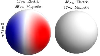
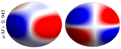
Figure 9: (color online). Perturbative horizon tendicities $\delta\mathcal{E}_{NN}$ and vorticities $\delta\mathcal{B}_{NN}$ for the $(2,2)$ quasinormal modes with electric and magnetic parities (see column labels at the top). The top row is for a Schwarzschild black hole, $a=0$; the bottom for a rapidly spinning Kerr black hole, $a/M=0.945$. The color intensity is proportional to the magnitude of the tendicity or vorticity, with blue (dark gray) for positive and red (light gray) for negative. For discussion, see Sec. III.1 of the text.

III.2 Equatorial-plane vortex and tendex lines, and vortexes and tendexes

As for the weak-field, radiative sources of Paper I, so also here, the equatorial plane is an informative and simple region in which to study the generation of gravitational waves.

For the (2,2) modes that we are studying, the $\delta\mathcal{E}_{jk}$ of an electric-parity perturbation and the $\delta\mathcal{B}_{jk}$ for magnetic parity are symmetric about the equatorial plane. This restricts two sets of field lines (tendex lines for electric-parity $\delta\mathcal{E}_{jk}$; vortex lines for magnetic-parity $\delta\mathcal{B}_{jk}$) to lie in the plane and forces the third to be normal to the plane. By contrast, the electric-parity $\delta\mathcal{B}_{jk}$ and magnetic-parity $\delta\mathcal{E}_{jk}$ are reflection antisymmetric. This requires that two sets of field lines cross the equatorial plane at $45^{\circ}$ angles, with equal and opposite eigenvalues (tendicities or vorticities), and forces the third set to lie in the plane and have zero eigenvalue; this third set of zero-vorticity vortex lines have less physical interest and so we will not illustrate them.

In this section, we shall focus on the in-plane field lines and their vorticities and tendicities.

III.2.1 Magnetic-parity perturbations of Schwarzschild black holes

In Sec. I.3.6 and Figs. 2 and 3, we discussed some equatorial-plane properties of the magnetic-parity $(2,2)$ mode. Here we shall explore these and other properties more deeply. Recall that for the magnetic-parity mode, the frame-drag field, and hence also the vortex lines and their vorticities, are fully gauge invariant.

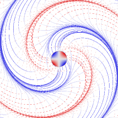
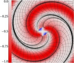
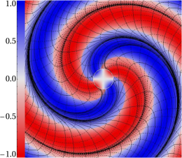
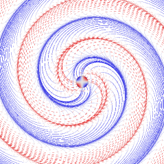
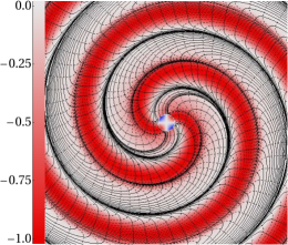
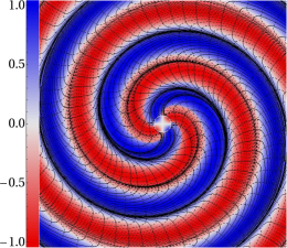
Figure 10: (color online). Three representations of the vortex lines and vortexes in the equatorial plane of a Schwarzschild black hole perturbed by a magnetic-parity $(2,2)$ quasinormal mode. The bottom panels span a region $56M$ on each side, and the top panels are a zoom-in of the lower panels, $30M$ on each side. All panels show positive-vorticity lines as solid and negative-vorticity lines as dashed. In all panels, blue (dark gray) corresponds to positive and red (light gray) to negative; the intensity of the color indicates the strength of the vorticity at that point normalized by the maximum of the vorticity at that radius (darker shading indicates a larger strength and lighter, weaker). Similarly, in all panels, the central circle surrounded by a narrow white line is the horizon colored by its vorticity as described above. Left column: Vortex lines colored and shaded by their scaled vorticity. Middle column: Negative vorticity coloring the plane with black vortex lines. Right column: Vorticity with the larger absolute value coloring the plane and black vortex lines. For discussion of this figure, see Sec. III.2.1.

In Fig. 10, we show six different depictions of the vortex lines and their vorticities in the equatorial plane, each designed to highlight particular issues. See the caption for details of what is depicted.

The radial variation of vorticity is not shown in this figure, only the angular variation. The vorticity actually passes through a large range of values as a function of radius: from the horizon to roughly $r=4M\simeq 1.5\lambdabar$ (roughly the outer edge of the near zone), the vorticity rapidly decreases; between $r\simeq 4M$ and $12M$ (roughly the extent of the transition zone), it falls off as $1/r$; and at $r\gtrsim 12M$ (the wave zone), it grows exponentially due to the damping of the quasinormal mode as time passes. (The wave field at larger radii was emitted earlier when the mode was stronger.) In the figure, we have removed these radial variations in order to highlight the angular variations.

By comparing the left panels of Fig. 10 with Fig 9 of Sec. VI D of Paper I, we see a strong resemblance between the vortex lines of our $(2,2)$, magnetic-parity perturbation of a Schwarzschild black hole, and those of a rotating current quadrupole in linearized theory. As in linearized theory, when the radial (or, synonymously, longitudinal) vortex lines in the near zone rotate, the effects of time retardation cause the lines, in the transition and wave zones, to collect around four backspiraling regions of strong vorticity (the vortexes) and to acquire perturbative tendex lines as they become transverse-traceless gravitational waves. The most important difference is that, for the black-hole perturbations, the positive vortex lines emerge from the blue, clockwise horizon vortexes and spiral outward (and the negative vortex lines emerge from the counterclockwise horizon vortexes) rather than emerging from a near-zone current quadrupole.

Although the left panels of Fig. 10 highlight most clearly the comparison with figures in Paper I, the middle and right panels more clearly show the relationship between the vortex lines (in black) and the vorticities, throughout the equatorial plane. In the middle panels (which show only the negative vorticity), the negative vortex lines that emerge longitudinally from the horizon stay in the center of their vortex in the near zone, and then collect onto the outer edge of the vortex in the transition and wave zones. Interestingly, near the horizon, there are also two weaker regions of negative vorticity between the two counterclockwise vortexes, regions associated with the tangential negative vortex lines that pass through this region without attaching to the horizon (and that presumably represent radiation traveling into the horizon).

In the right panels of Fig. 10 (which show the in-plane vorticity with the larger absolute value), a clockwise vortex that extends radially from the horizon takes the place of the weaker region of counterclockwise vorticity. From these panels, it is most evident that the vortexes and vortex lines of opposite signs are identical, though rotated by $90^{\circ}$. These panels also highlight that there are four spirals of nearly zero vorticity that separate the vortexes in the wave zone, which the spiraling vortex lines approach. All three vorticities nearly vanish at these spirals; in the limit of infinite radius, they become vanishing points for the radiation, which must exist for topological reasons Zimmerman et al. (2011).

III.2.2 Gauge dependence of electric-parity tendexes for a Schwarzschild black hole

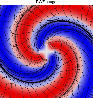
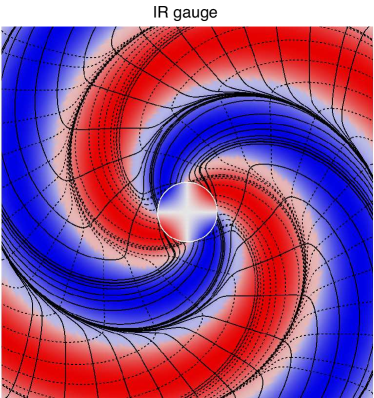
Figure 11: (color online). The equatorial-plane, electric-parity tendexes and tendex lines of a $(2,2)$ perturbation of a Schwarzschild black hole in RWZ gauge (left panel) and IR gauge (right panel). The conventions for the lines, the coloring and the shading are identical to those in the right panels of Fig. 10.

In this subsection, we explore the gauge dependence of the (2,2) modes for a Schwarzschild black hole. In Sec. II.3, we showed that for magnetic-parity modes, all gauges share the same slicing. Therefore, to maximize any gauge dependence that there might be, we focus on the electric-parity (2,2) mode.

Because the frame-drag field of the unperturbed Schwarzschild black hole vanishes, this mode’s perturbative frame-drag field will be unaffected by perturbative changes of the spatial coordinates. Therefore, we focus on the perturbative tidal field $\delta\bm{\mathcal{E}}$ of the electric-parity mode, which is sensitive to both perturbative slicing changes and perturbative spatial coordinate changes.

In Fig. 11, we plot this field’s perturbative equatorial tendexes and tendex lines for the electric-parity (2,2) mode in RWZ gauge (left panel) and IR gauge (right panel)—which differ, for this mode, in both slicing and spatial coordinates. The tendex lines for the two gauges were seeded at the same coordinate points, so all the differences between the panels can be attributed to the gauge differences.

The two panels are almost identical. Therefore, these maximally sensitive tendexes and tendex lines are remarkably unaffected by switching from one gauge to the other. The primary differences are that (i) the tendex lines of IR gauge which are near the black hole tend to be pulled closer to the horizon as compared to RWZ gauge (ii) the lines falling onto the attracting spiral are bunched even more tightly in IR gauge than in RWZ gauge; however, more lines reach the spiral in RWZ gauge in this figure, and (iii) the four tendex spirals wind more tightly in IR gauge, which is most easily seen by comparing the lower right and upper left corners of the two panels.

One subtlety that must be remarked upon is that the central circle colored by the normal-normal component of the tidal field (surface tendicity) in the RWZ gauge (left panel of Fig. 11) is simply the surface $r=2M$, and not the true event horizon. The location of the event horizon is affected by the perturbations in a gauge-dependent manner, as discussed by Vega, Poisson, and Massey Vega et al. (2011). We rely on the results of this article in the brief discussion that follows. In RWZ gauge, the horizon is at $r_{H}=2M+\delta r(\tilde{t},\theta,\phi)$, where the function $\delta r$ can be solved for by ensuring that the vector tangent to the perturbed generators (in our case, $l^{\mu}=\partial x^{\mu}/\partial\tilde{t}$) remains null Vega et al. (2011). We give an expression for $\delta r$ in Appendix A.5. There we also discuss the correction to the horizon tendicity in RWZ gauge. One key result is that the horizon tendicity has the same angular distribution in RWZ gauge as in IR gauge (given by the $Y^{22}$ spherical harmonic), so that the normal-normal tendicity on the horizon and on the surface at $r=2M$ differ only by an amplitude and phase in RWZ gauge. Meanwhile, in IR gauge the horizon remains at $r_{H}=2M$ and so the colored central circle is in fact the horizon, colored by its horizon tendicity.

However, the bulk tendexes and tendex lines are determined completely independently of these horizon considerations, and so Fig. 11 provides an accurate comparison of them in the two gauges.

III.2.3 Duality and influence of spin in the equatorial plane

In this subsection, we use Fig. 12 to explore duality and the influence of spin, for the fundamental $(2,2)$ mode.

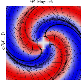
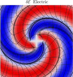
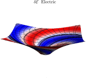
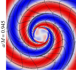
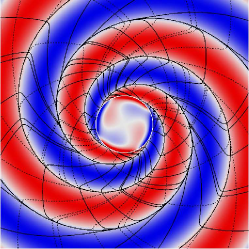
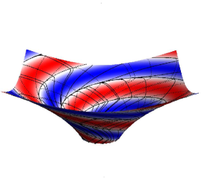
Figure 12: (color online). Vortexes and tendexes and their field lines in the equatorial plane for $(2,2)$ modes of Schwarzschild and Kerr black holes. The lines, the coloring and the shading are identical to those in the right panels of Fig. 10. The upper row is for a Schwarzschild black hole $(a=0)$; the lower row, for a rapidly spinning Kerr black hole $(a=0.945)$; see labels on the left. The left column shows the vortex lines and vorticities for magnetic parity (which are gauge invariant for the perturbations of a Schwarzschild hole); the middle and right columns show the tendex lines and tendicities for the electric-parity mode in IR gauge; see labels at the top. In the right column, the equatorial plane is isometrically embedded in three-dimensional Euclidean space. The top panels are $24M$ across; the bottom, $14M$. This figure elucidates duality and the influence of black-hole spin; see the discussion in Sec. III.2.3.

By comparing the left and center panels in the top row of Fig. 12, we see visually the near duality between the electric- and magnetic-parity modes for a Schwarzschild hole. This near duality is explored mathematically in App. C. Specifically, the vortexes and their lines for the magnetic-parity mode (left) are nearly identical to the tendexes and their lines for the electric-parity mode. The only small differences appear in the size of the nearly zero-vorticity (or tendicity) regions, and the curvatures of the lines.

For the fast-spinning Kerr black hole (the bottom left and center panels of Fig. 12), the near duality is still obvious, especially in the colored vortexes and tendexes; but it is less strong than for Schwarzschild, especially in the field lines. The vortex lines (on the left) continue to look like those of a Schwarzschild black hole, but the tendex lines (in the middle) curve in the opposite direction, which makes some lines reach out from the horizon and connect back to it instead of spiraling away from the horizon.

By comparing the top and bottom panels in the left and center columns of Fig. 12, we see the influence of the background black hole’s spin on the dynamics of the perturbative vortexes and tendexes. For fast Kerr (bottom), the vortexes and tendexes near the horizon look more transverse (less radial) than for Schwarzschild, because the size of the near zone is much smaller. (The frequency of the waves is nearly twice that for a perturbed Schwarzschild hole.) The higher frequency also explains why the spirals of the vortexes and tendexes are tighter.

In the isometric embedding diagrams in the right column of Fig. 12, we see that proper radial distance in the near zone is somewhat larger than it appears in the flat, planar drawing. Taking this into account, we conclude that, aside from a few small differences, the qualitative ways in which waves are generated for fast Kerr and for Schwarzschild are the same: two pairs of vortexes or tendexes emerge longitudinally from horizon vortexes, and twist into backward spirals that eventually form the transverse-traceless gravitational waves.

III.2.4 Vortexes of electric-parity mode, and perturbative tendexes of magnetic-parity mode for a Schwarzschild black hole

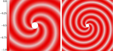
Figure 13: (color online). For an electric-parity (2,2) mode of a Schwarzschild black hole: the vorticity of the counterclockwise vortex lines that pass through the equatorial plane at a 45 degree angle. The clockwise vortex lines that pass through the plane have equal and opposite vorticity. By near duality, this figure also depicts the perturbative tendex structure for the magnetic-parity (2,2) mode. The conventions for coloring and shading are the same as in Fig. 10. Because the horizon vorticity is exactly zero for this mode, the horizon is shown as a white disk. The left panel, a region $30M$ across, is a zoom in of the right panel, which is $56M$ across.

In Fig. 13, we visualize the vortexes of the electric-parity $(2,2)$ mode of a Schwarzschild hole. (By near duality, the perturbative tendexes of the magnetic-parity mode must look nearly the same.)

As noted at the beginning of Sec. III.2, reflection antisymmetry of the frame-drag field for this electric-parity mode dictates that through each point in the plane there will pass one zero-vorticity vortex line lying in the plane, and two vortex lines with equal and opposite vorticities that pass through the plane at 45 degree angles and are orthogonal to each other and to the zero-vorticity line. The vorticity plotted in Fig. 13 is that of the counterclockwise, 45 degree line. For the clockwise line, the vorticity pattern is identically the same, but blue instead of red.

There are again four regions of strong vorticity (four vortexes), which spiral outward from the horizon, becoming gravitational waves. In this case, the four regions look identical, whereas for the tendexes of this same electric-parity mode (middle column of Fig. 12) there is an alternation between blue and red. There is actually an alternation here, too, though it does not show in the figure: The relative tilt of the lines (in the sense of the $\phi$ direction) rotates, such that in one tendex, the red tendex lines pass through the plane with a forward 45 degree tilt on average, and in the next tendex, with a backward 45 degree tilt; and conversely for the blue tendex lines.

III.3 Three-Dimensional vortexes and tendexes

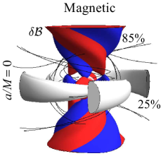
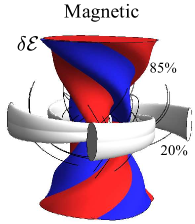
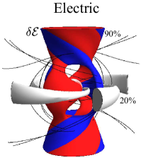
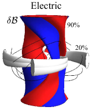
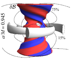
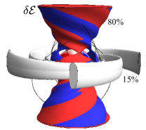
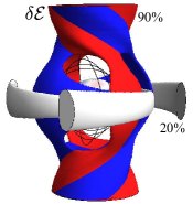
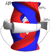
Figure 14: (color online). Three-dimensional vortexes and tendexes of the same four modes as are shown in Fig. 12. As there, so here, the top row is for a Schwarzschild black hole, and the bottom for fast-spin Kerr, $a=0.945$; the left two columns (one in Fig. 12) are for a magnetic-parity (2,2) mode (with the vortexes in IR coordinates), and the right two columns (one in Fig. 12) are for electric parity in IR gauge. For each parity, the first column shows structures of the field that generates the waves ($\delta\mathcal{B}$ for magnetic parity; $\delta\mathcal{E}$ for electric parity) and the second column shows structures of the other field (not included in the equatorial-plane drawings of Fig. 12). In each panel, the colored surfaces show the outer faces of vortexes (for $\delta\mathcal{B}$) or tendexes (for $\delta\mathcal{E}$), defined as the locations, for a given radius, where the largest-in-magnitude eigenvalue of the field being plotted ($\delta\mathcal{B}$ or $\delta\mathcal{E}$) has dropped to a certain percentage (90, 85, 80 or 75) of its maximum for that radius; that percentage is shown alongside the colored surfaces. As in previous figures, the surface is red (light gray) if that largest-in-magnitude eigenvalue is negative and blue (dark gray) if positive. The off-white regions are surfaces where the largest-in-magnitude eigenvalue has dropped to 15%, 20% or 25% of the maximum at that radius. In each panel the black lines are a few of the vortex lines (for $\delta\mathcal{B}$ panels) or tendex lines (for $\delta\mathcal{E}$ panels) that become transverse when they reach large radii, and thereby produce the tidal or frame-drag force of an emitted gravitational wave. For discussion of this figure, see Sec. III.3.

In this section, we shall explore the 3-dimensional vortexes and tendexes of the $(2,2)$ modes of Schwarzschild and Kerr black holes, which are depicted in Fig. 14. In the first subsection, we shall focus on what this figure tells us about the generation of gravitational waves, and in the second, what it tells us about duality.

III.3.1 Physical description of gravitational-wave generation

In Sec. I.3.6 of the Introduction, we summarized in great detail what we have learned about gravitational-wave generation from our vortex and tendex studies. There we focused on the $(2,2)$ magnetic-parity mode, and among other things we scrutinized the upper left panel of Fig. 14 (which we reproduced as Fig. 4). Here, instead, we shall focus on the $(2,2)$ electric-parity mode as depicted in the right half of Fig. 14.

We begin with the perturbative tendexes of the electric-parity, (2,2) mode of a Schwarzschild black hole (third panel on top row of Fig. 14). The 3-D tendexes emerge from the horizon as four deformed-cylinder structures, two red (light gray) and two blue (dark gray). These are the extensions into the third dimension of the four near-zone, equatorial-plane tendexes of the center panel in Fig. 12 above. As we enter the transition zone, the four 3D tendexes lengthen vertically (parallel to the poles), and then as we enter the wave zone, they spiral upward and downward around the poles; they have become gravitational waves. They are concentrated near the poles because the (2,2)–mode gravitational waves are significantly stronger in polar directions than in the equator.

In this panel, we also see black tendex lines that emerge from the horizon and spiral upward and downward alongside the polar-spiraling tendexes, becoming nearly transverse at large radii—part of the outgoing gravitational waves. Of course, there are similar tendex lines, not shown, inside the spiraling tendexes. In addition, we also see tendex lines in the inner part of the wave zone that are approximately polar circles; these are also part of the outgoing waves.

The top rightmost panel depicts the vortexes associated with this electric-parity mode. The horizon vorticity vanishes, so the horizon is white. The vortexes near the horizon are dominated by the longitudinal-transverse part of the frame-drag field $\bm{\mathcal{B}}^{\rm LT}$, which interacts with $\delta\bm{\mathcal{E}}^{\rm L}$ and $\delta\bm{\mathcal{E}}^{\rm LT}$ to maintain their joint near-zone structure as they rotate (cf. the description of the dual magnetic-parity mode in Sec. I.3.6). However, of course, there is also a $\bm{\mathcal{B}}^{\rm TT}$ associated with the ingoing gravitational waves. At large radii, in the outgoing-wave zone, the vortexes, like the tendexes of the third panel top row, spiral upward and downward around the polar axis; they have joined with the tendexes to form the full gravitational-wave structure.

For insight into how (we think) the near-zone tendexes of this electric-parity mode, extending radially out of the horizon, generate these outgoing gravitational waves, and how the ingoing waves, that they also generate, act back on them and drive their gradual decay, see the description of this mode’s dual in Sec. I.3.6.

For the rapid-spin Kerr black hole, the tendex and vortex structures (last two panels of second row of Fig. 14) are quite similar to those for the Schwarzschild black hole. The detailed differences are similar to those in the equatorial plane (see discussion in Sec. III.2.3 above): smaller near zone and tighter spiraling for the tendexes because of the higher eigenfrequency; nonvanishing horizon vorticity with a predominantly $Y^{32}(\theta,\phi)$ angular structure. In the near zone, the 3D vortexes seem to have acquired a longitudinal (radial) part, emerging from the $Y^{32}$ horizon vortexes (though this is largely hidden behind the off-white structures). Thus, for a Kerr black hole, one might intuitively describe the generation of gravitational waves as being produced by a superposition of near-zone tendexes that induce vortexes by their motions, and near-zone vortexes that induce tendexes by their motions. However, because the near-zone vortexes are weaker than the tendexes, the tendexes still play the dominant role for gravitational-wave generation in this electric-parity mode.

III.3.2 Approximate duality

By comparing the magnetic-parity left half of Fig. 14 with the electric-parity right half, we can visually assess the degree to which there is a duality between the modes in three dimensions. For the perturbations of Schwarzschild black holes (top row), the most notable difference between the magnetic- and electric-parity perturbations is that the transition between the longitudinal near-zone and spiraling wave-zone vortexes of the magnetic-parity perturbation is more abrupt, and happens closer to the horizon than it does in the electric-parity perturbations. The reason for this is encoded in Eqs. (90), (91), and (92), but we do not have a simple physical explanation for why this occurs. This difference is magnified for perturbations of the rapidly rotating Kerr black hole (bottom row). Thus, the small breaking of duality quantified in App. C for Schwarzschild black holes seems to be more pronounced in three-dimensions than in two, and stronger for rapidly rotating black holes than for non-rotating ones.

Nevertheless, the qualitative picture of wave generation by longitudinal near-zone tendexes and vortexes is essentially dual for perturbations of the two parities.

III.4 Comparing vortex lines of a perturbed Kerr black hole and a binary-black-hole-merger remnant

   

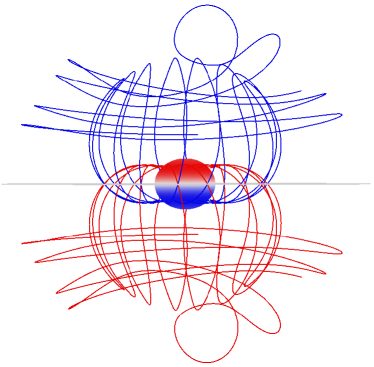
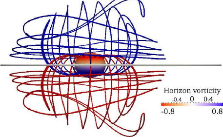
Figure 15: (color online). Left: Vortex lines of a $a/M=0.945$ Kerr black hole perturbed by an electric-parity $(2,2)$ quasinormal-mode in IR gauge. Right: Vortex lines from a $a/M=0.945$ ringing down Kerr black hole obtained from a numerical simulation Lovelace et al. (2012) of two identical merging black holes with spins of magnitude $0.97$ aligned parallel to the orbital angular momentum. In the simulation, we chose a late enough time that the common apparent horizon is essentially that of a single, perturbed black hole, and we computed the vortex lines using methods summarized in Ref. Owen et al. (2011).

As a conclusion to this section and a prelude to future work, in Fig. 15 we compare the vortex lines found using our analytic methods to those found in a numerical ringdown of a fast-spinning Kerr black hole.

More specifically, we compare an electric-parity, $(2,2)$ quasinormal-mode perturbation of a Kerr black hole with dimensionless spin $a/M=0.945$, to a ringing-down Kerr black hole of the same spin formed in a numerical simulation Lovelace et al. (2012) of the merger of two equal-mass black holes with equal spins of magnitude 0.97 aligned with the orbital angular momentum. (Note that because of the symmetry of this configuration, during the ringdown there is no magnetic-parity $(2,2)$ mode excited.)

For both the analytical and numerical calculations, the vortex lines are those of the full frame-drag tensor. To describe the magnitude of the perturbation in the analytical calculation, we write the frame-drag field as $\mathcal{B}_{\hat{i}\hat{j}}=\mathcal{B}_{\hat{i}\hat{j}}^{(0)}+\mathcal{B}_{\hat{i}\hat{j}}^{(1)}$, including the background part $\mathcal{B}_{\hat{i}\hat{j}}^{(0)}$ and the perturbation $\mathcal{B}_{\hat{i}\hat{j}}^{(1)}\equiv\delta\mathcal{B}_{\hat{i}\hat{j}}$ (as in App. F). We choose the ratio of the maximum of the perturbation of the horizon vorticity, $\mathcal{B}_{NN}^{(1)}$ to the background horizon vorticity $\mathcal{B}_{NN}^{(0)}$ to be of order $10^{-3}$. This amplitude of the perturbation produces lines that agree qualitatively with those from the numerical simulation.

The lines of the full frame-drag field look quite different from those for just $\delta\mathcal{B}_{\hat{i}\hat{j}}$ depicted in Figs. 12 and 14. Near the equator, the vortex lines in both panels look like those of an unperturbed Kerr black hole (see Paper II). Closer to the axis of rotation, the background vortex lines become degenerate, and the perturbations break the degeneracy by picking the principal axes of the perturbative field. Correspondingly, near the rotation axis and at large enough radii to be in or near the wave zone, the vortex lines resemble those of transverse-traceless gravitational waves, which are emitted symmetrically above and below the hole.

Although the vortex lines from these similar physical situations were computed using very different methods and gauge conditions, the results are qualitatively similar (see Fig. 15). The lines in the two figures are not identical, but they were selected to intersect the horizon in approximately the same places; a careful inspection shows there are small differences, for example very near the horizon.

This comparison ultimately gives us confidence that our analytical methods can guide our understanding of the vortexes and tendexes in the late stages of numerical simulations.

IV Superposed $(2,2)$ and $(2,-2)$ Quasinormal Modes of Schwarzschild

IV.1 Magnetic-parity superposed modes

In Sec. I.3.9, we summarized the properties of the quasinormal mode of Schwarzschild that is obtained by superposing the magnetic-parity $(2,2)$ and $(2,-2)$ modes. Here we give details. The vortex lines and vorticities for this superposed mode are depicted in Fig. 16 using the three types of visualizations in Fig. 10.

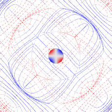
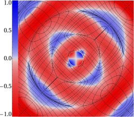
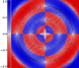
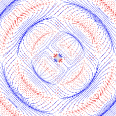
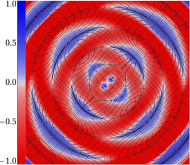
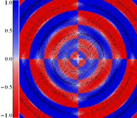
Figure 16: (color online). The vorticities and vortex lines in the equatorial plane of a Schwarzschild black hole, for the fundamental magnetic-parity $(2,2)$ mode superposed on the fundamental magnetic-parity $(2,-2)$ mode, depicted using the same three visualization techniques as in Fig. 10. Here, however, we do not scale the vorticity by any function, but the numbers on the vorticity scale on the left of the panels are equal to $\sqrt{{\rm vorticity}\times r}$ (where $r$ is radius), in units of the maximum value of this quantity, which occurs on the horizon at $\phi=3\pi/4$ and $\phi=7\pi/4$. The top panels cover a region $30M$ across, and the bottom panels are a zoom-out of the upper panels, $56M$ across. The central circle in all panels is the horizon as viewed from the polar axis, colored by its vorticity. Left column: The two families of vortex lines (one shown dashed, the other solid) with each line colored, at each point, by the sign of its vorticity (blue [dark gray] for positive, i.e., clockwise; red (light gray) for negative, i.e., counterclockwise), and each line has an intensity proportional to the magnitude of its vorticity. Center column: The same vortex lines are colored black, and the equatorial plane is colored by the vorticity of the dashed family of lines. Right column: The same as the center column, but the equatorial plane is colored by the vorticity with the larger magnitude.

The left column of Fig. 16 shows the two families of vortex lines that lie in the equatorial plane, color coded by their vorticities. The solid-line family has predominantly positive (clockwise) vorticity, but in some regions its vorticity becomes weakly negative (counterclockwise). The dashed-line family has predominantly negative vorticity, but in some regions it is weakly positive. A rotation around the hole by angle $\pi/2$ maps each family into the other.

In the center column of Fig. 16, the vortex lines are drawn black and the equatorial plane is colored by the vorticity of the dashed lines. To deduce the coloring for the solid lines, just rotate the colored plane (but not the lines) by $\pi/2$ and interchange red (light gray) and blue (dark gray). By contrast with most previous figures, the radial variation of the vorticity is not scaled out of this figure; so in the wave zone (roughly, the outer half of right panel) the coloring oscillates radially, in color and intensity, in the manner of a gravitational wave. At large radii, there is also a growth of intensity (and saturation of the color scale) due to the waves emitted earlier having larger amplitude.

In the right column of Fig. 16, the vortex lines are again drawn black, and the equatorial plane is now colored by the larger of the two vorticities in amplitude.

Together, the columns of Fig. 16 provide the following picture: For each family of lines, the equatorial-plane vortexes form interleaved rings (dashed lines and red [light gray] vortexes for center column). Most of the family’s vortex lines form closed, distorted ellipses that, when tangential, lie in a single vortex (red for dashed lines), and when more nearly radial, travel from one vortex to another. In the wave zone, these line and vortex structures grow longer tangentially as they propagate outward, and they maintain fixed radial thickness. When one looks at both families simultaneously, focusing on the strongest at each point (right column), one sees vortexes of alternating red and blue vorticity (light and dark gray). The angular oscillations are those of a quadrupolar structure; the radial oscillations are those of a propagating wave.

In the near zone, the vortex lines have rather sharp, right angled features associated with the quadrupolar nature of the near-zone perturbation; this is to be compared to the oscillating current quadrupole in linearized gravity (Paper I, Sec. VI, Fig. 15). There are multiple singular points in the lines, degenerate points where three lines cross with sharp bends, and where both families of vortex lines take on the same eigenvalue. (The third eigenvalue, that of the lines perpendicular to the plane, must then be minus twice the vorticity of these lines, in order for the sum of the eigenvalues to vanish).

We shall discuss the dynamics of these vortex lines and vortexes in Sec. IV.3 below, after first gaining insight into the electric-parity superposed mode (whose vortexes will teach us about this magnetic-parity mode’s tendexes through the near duality).

IV.2 Electric-parity superposed mode

For the mode constructed by superposing electric-parity (2,2) and (2,-2) modes of Schwarzschild, as for the electric-parity (2,2) mode itself (Sec. III.2.4), symmetry considerations dictate that: (i) one family of vortex lines lies in the equatorial plane and has vanishing vorticity, (ii) two families pass through the equatorial plane at $45^{\circ}$ angles, with equal and opposite vorticities, and (iii) the horizon vorticity vanishes.

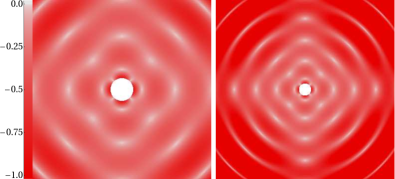
Figure 17: (color online). For the electric-parity, superposed (2,2) and (2,-2) fundamental modes of Schwarzschild: the vorticity of the counterclockwise vortex lines that pass through the equatorial plane at $45^{\circ}$ angles. By near duality, this figure also depicts the perturbative tendex structure for the magnetic-parity superposed mode. The intensity scale of the red color (left edge of figure) is the same as that in the center column of Fig. 16. The left panel, a region $30M$ across, is a zoom-in of the right panel, which is $56M$ across. This figure is the superposed-mode analog of Fig. 13.

In Fig. 17 [analog of Fig. 13 for the (2,2) electric-parity mode], we show the vorticity of the family of counterclockwise vortex lines, as they pass through the equatorial plane.

In the near zone of this figure, we see again a distinct quadrupolar structure, with four lobes of strong vorticity present near the horizon (four near-zone vortexes). Beyond these near-zone lobes, there is a ring of vanishing vorticity, followed by an annulus where the cast-off vortexes of a previous cycle have begun to deform into an annulus of stronger vorticity. In the wave zone, the vortexes have transitioned into outward traveling transverse waves, with regions of vanishing vorticity between the crests and troughs of each wave. The waves are strongest along the diagonals, though in the near zone the (LT) frame-drag field is strongest in the up, down, left and right directions.

By (near) duality, the tendexes of the magnetic-parity superposed mode will have the same form as these electric-parity-mode vortexes. Accordingly, in the next section, we will use this figure to elucidate the magnetic-parity mode’s dynamics — and by duality, also the dynamics of this electric-parity mode.

IV.3 Dynamics of the magnetic-parity superposed mode

We now turn to the dynamics of the magnetic-parity superposed mode, which we studied in Sec. IV.1

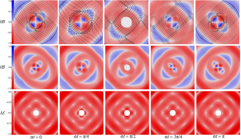
Figure 18: (color online). Time evolution of the equatorial vortexes (top and middle rows) and equatorial perturbative tendexes (bottom row) for the superposed $(2,2)$ and $(2,-2)$ magnetic-parity mode of Schwarzschild in RWZ gauge. The color scale is the same as the center column of Fig. 16, and the gravitational-wave-induced exponential decay of the vorticity and tendicity has been removed. Top row: Equatorial vortex lines and their vorticity plotted in a region near the horizon ($16M$ across) followed over time $t$. The real part of the eigenfrequency is denoted $\sigma$, so the successive panels, left to right cover half a cycle of the mode’s oscillation. Middle row: The vorticity of the equatorial vortex lines in the near, intermediate and beginning of wave zone ($30M$ across) at the same time steps as the top row. Bottom row: Tendicity of the counterclockwise tendex lines passing through the equatorial plane (which is dual to the left panel of Fig. 17), plotted at the same time steps as the top row.

In Fig. 18 for this mode we show, in the equatorial plane, the time evolution of (i) the vortex lines and their vorticities near the black hole (top row), and (ii) on a larger scale that extends into the wave zone, the mode’s vortexes (middle row) and perturbative tendexes (bottom row). The five panels in the top row are stills from a movie at Osc . To be absolutely clear, the vortexes and tendexes are those of the same magnetic-parity mode. As in the center column of Fig. 16, the top and middle rows show only one family of vortexes, that for the dashed vortex lines which have predominantly negative vorticity; and as in Fig. 17, the bottom row shows only the tendicity of the negative-tendicity perturbative tendexes that pass through the equatorial plane at $45^{\circ}$. Time $t=0$ (left panels of Fig. 18) is chosen at a moment when the horizon vorticity is maximum, whereas Figs. 16 and 17 are snapshots at the slightly earlier time $\sigma t\approx-\pi/3$ (which gives nearly the same vortex structures as the fourth column, after a rotation by $\pi/2$).

In interpreting Fig. 18, especially the top row, we emphasize that there is no unique way of following a single vortex or tendex line in time. The same is true of electric and magnetic field lines in Maxwell’s theory (cf. Belcher and Olbert (2003)). While we hope to elucidate this issue in future work, here, in constructing the panels in the top row of Fig. 18, we have simply started the integration of the vortex lines from the same points at each time step, making no attempt to identify and follow individual lines from moment to moment. Correspondingly, in order to interpret Fig. 18 and gain insight into the dynamics of the superposed mode, instead of trying to follow individual lines, we will focus on the lines’ evolving shapes, and the structures of the vortexes and tendexes and the equations governing their evolution on the horizon.

As a foundation for understanding the near-zone dynamics depicted in this figure, we write down explicit expressions for the longitudinal and longitudinal-transverse parts of the frame-drag and tidal fields on the horizon:

$$\mathcal{B}_{\hat{r}\hat{r}} = \Re\left[{3\over 2i\omega M^{3}}e^{-i\omega(\tilde{t}+2M)}\right]\mathcal{Y}(\theta,\phi)\;,$$ (26a)

$$\mathcal{B}_{\hat{r}\hat{A}} = \Re\left[{1\over 2\sqrt{2}M^{2}}(1-\beta)e^{-i\omega(\tilde{t}+2M)}\right]D_{\hat{A}}\mathcal{Y}\;,$$ (26b)

$$\mathcal{\delta}E_{\hat{r}\hat{A}} = \Re\left[{1\over 2\sqrt{2}M^{2}}(1+\beta)e^{-i\omega(\tilde{t}+2M)}\right]\left(-{\epsilon_{\hat{A}}}^{\hat{B}}D_{\hat{A}}\right)\mathcal{Y}\;,$$

where

$$\beta\equiv{3\over 2i\omega M(1-4i\omega M)}\;.$$ (26d)

Here the normalization is that of App. A, $\omega=(0.37367-0.08896i)/M$ is the mode’s eigenfrequency, ${\epsilon_{\hat{A}}}^{\hat{B}}$ is the Levi-Civita tensor on the horizon,

$$\mathcal{Y}\equiv Y^{22}+Y^{2\,-2}=\sqrt{15/8\pi}\sin^{2}\theta\cos 2\phi$$ (26e)

is this mode’s scalar spherical harmonic, and $D_{\hat{A}}$ is the covariant derivative on the unit 2-sphere (related to the covariant derivative on the horizon by $D_{\hat{A}}=2M\bm{\nabla}_{\hat{A}}$). [Equations (26e) follow from Eqs. (A.2), (LABEL:Qanalytic), (54) of App. A, the vector-spherical-harmonic definitions (83a) and (87a), and definition (5) of the EF time coordinate.]

Equations (26e) are the fields measured by Eddington-Finkelstein observers. The conservation law (4a) for longitudinal field lines threading the horizon (which we shall need below) involves, by contrast, the LT frame-drag field measured by Schwarzschild observers on the “stretched horizon” (very close to the event horizon). Since the Schwarzschild observers move outward with velocity $\bm{v}=(2M/r)\bm{N}\simeq\bm{N}$ with respect to the EF observers, and with $\gamma\equiv 1/\sqrt{1-v^{2}}\simeq 1/(\sqrt{2}\alpha)$, the field they measure is $\bm{\mathcal{B}}^{\rm LT}_{\rm Sch}=\gamma(\bm{\mathcal{B}}^{\rm LT}-\bm{N}\times\delta\bm{\mathcal{E}}^{\rm LT})$. This field diverges as $1/\alpha$ as the stretched horizon is pushed toward the event horizon; to remove that divergence, in the Membrane Paradigm Thorne et al. (1986)) we renormalize by multiplying with $\alpha$:

$${\mathcal{B}}^{\rm H}_{\hat{r}\hat{A}} \equiv \alpha\bm{\mathcal{B}}^{\rm LT}_{\rm Sch}=\alpha\gamma(\bm{\mathcal{B}}^{\rm LT}-\bm{N}\times\delta\bm{\mathcal{E}}^{\rm LT})$$ (27)

$$= \Re\left[{1\over 4M^{2}}e^{-i\omega(\tilde{t}+2M)}\right]D_{\hat{A}}\mathcal{Y}\;.$$

The second line is obtained by inserting the EF fields (26a) and (26b), and $\gamma=1/\sqrt{2}\alpha$, into the first line. The conservation law for longitudinal vortex lines threading the horizon (actually, one of the Maxwell-like Bianchi identities in disguise) says that

$$\partial\mathcal{B}_{NN}/\partial\tilde{t}+\nabla_{\hat{A}}(-\mathcal{B}^{\rm H}_{\hat{r}\hat{A}})=0\;;$$ (28)

cf. Eq. (4a) and subsequent discussion. (In this Schwarzschild-perturbation-theory case, there are no small spin-coefficient terms to spoil the perfection of the conservation law.) The vortex-line density and flux expressions (26a) and (27) do, indeed, satisfy this conservation law, by virtue of the fact that the 2-dimensional Laplacian acting on the quadrupolar spherical harmonic $\mathcal{Y}$ gives $D_{\hat{A}}D^{\hat{A}}\mathcal{Y}=-6\mathcal{Y}$.

Equations (26e) and (28) tell us the following: (i) On and near the horizon, the LT fields $\bm{\mathcal{B}}^{\rm LT}$ [Eq. (26b)] and $\delta\bm{\mathcal{E}}^{\rm LT}$ [Eq. (LABEL:eq:ErAHsuperposed)], and also $\mathcal{B}^{\rm H}_{\hat{r}\hat{A}}$ [Eq. (27)], all oscillate approximately out of phase with the longitudinal field $\bm{\mathcal{B}}^{\rm L}$ [Eq. (26a)]. Therefore, near-zone energy is fed back and forth between the L and LT fields as the black hole pulsates.

(ii) The conservation law (28) says that, if we regard $\mathcal{B}_{NN}$ as the density of vortex lines of $\bm{\mathcal{B}}^{\rm L}$ threading the horizon, and $-\mathcal{B}^{\rm H}_{\hat{r}\hat{A}}$ as the flux of vortex lines (number crossing a unit length in the horizon per unit time), then these horizon-threading vortex lines of $\bm{\mathcal{B}}^{\rm L}$ are conserved during the pulsation. More specifically:

(iii) As the mode evolves in Fig. 18 from $\sigma t=0$ to $\sigma t=\pi$, the conserved vortex lines are pushed away from the center of each horizon vortex toward its white edges, and there the conserved lines from the red region (counterclockwise) annihilate with the conserved lines from the blue region (clockwise). The pushing is embodied in the vortex-line flux $-\mathcal{B}^{\rm H}_{\hat{r}\hat{A}}$, which grows stronger during this evolution.

(iv) As the mode evolves further from $\sigma t=\pi/2$ to $\sigma t=\pi$, conserved vortex lines of $\bm{\mathcal{B}}^{\rm L}$ are created in pairs (one clockwise, the other counterclockwise) at the white edges of the horizon vortexes, and move inward toward the center of each vortex.

Turn, now, from the conserved vortex lines of $\bm{\mathcal{B}}^{\rm L}$ piercing the horizon to the 3D vortex lines outside the horizon, depicted in the top row of Fig. 18. Because these are lines of the full 3D frame-drag field $\bm{\mathcal{B}}$ and not its longitudinal part $\bm{\mathcal{B}}^{\rm L}$, they do not obey a conservation law and there is no unique way of following individual lines from one panel to the next. However, their evolving shapes teach us much about the geometrodynamics of this superposed mode:

At time $\sigma t=0$ (upper left panel), the horizon-piercing vortex lines of the full frame-drag field $\bm{\mathcal{B}}$ are almost perfectly radial, with clockwise (solid) tendex lines emerging from the two blue horizon tendexes, and counterclockwise (dashed) tendex lines emerging from the two red horizon tendexes. As time passes, the horizon piercing lines become less radial and the horizon vorticity decreases ($\sigma t=\pi/4$) until the lines’ angles to the horizon are almost all near $45^{\circ}$ and the horizon vorticity vanishes ($\sigma t=\pi/2$). Note that the lines that lie precisely on the diagonals, and which contact the horizon radially in the middle panel ($\sigma t=\pi/2$), have zero vorticity where they strike the horizon. This latter fact allows them to have a more radial angle of intersection than almost all other lines. The near-horizon frame-drag field has evolved at this time from being predominantly longitudinal, $\bm{\mathcal{B}}^{\rm L}$, to being predominantly longitudinal-transverse, $\bm{\mathcal{B}}^{\rm LT}$, but with some small admixture of transverse-traceless ingoing waves, $\bm{\mathcal{B}}^{\rm TT}$. As time moves onward from $\sigma t=\pi/2$ to $\sigma t=\pi$, the vortex lines in the outer part of each panel reach around on the horizon and attach to a quadrant on the side rather than directly below themselves—a quadrant that has newly acquired the color corresponding to the lines’ own vorticity (blue for solid lines, red for dashed lines).

At $\sigma t=0$ (upper left panel), the near-horizon, nearly circular vortex lines in each quadrant represent, predominantly, the transverse-isotropic part of $\bm{\mathcal{B}}^{\rm L}$ and keep it trace free. As time passes and $\bm{\mathcal{B}}^{\rm L}$ decreases,we can regard these lines as traveling outward, forming the distorted ellipses which become gravitational waves in the far zone. The manner in which these circular vortex lines are restored each cycle appears to be as follows: As discussed above, as the horizon vorticity oscillates through zero, formerly longitudinal lines are pushed away from their respective vortexes and become first more longitudinal-transverse, and then attach to a different quadrant of the horizon; meanwhile the $\bm{\mathcal{B}}^{\rm L}$ is being regenerated with opposite sign in each quadrant, which requires new transverse-isotropic lines of opposite vorticity. These lines run tangent to the horizon, hugging it while they cross through a vortex of strong opposite vorticity. At each edge of the vortex these isotropic-transverse lines link up with predominantly radial lines which have the same sign of vorticity (it appears that it is the degenerate points at these edges that allow for such a reconnection). This deforms the highly distorted, nearly circular arcs, which then lift off the horizon and propagate away as the cycle progresses.

This entire evolution is being driven by the oscillatory turn-off and turn-on of the longitudinal part of the frame-drag field $\bm{\mathcal{B}}^{\rm L}$.

Turn attention to the evolution of the mode’s equatorial vortexes (middle row) and tendexes (bottom row). In accord with our discussion above of the evolution of the horizon fields, Eqs. (26e), these panels reveal (see below) that the vortexes and tendexes oscillate out of phase with each other. Near-zone energy (see footnote 1 in Sec. I.3.8) gets fed back and forth between vortexes and tendexes in an oscillatory manner (though during this feeding, some of it leaks out into the transition zone and thence into gravitational waves). This oscillatory feeding enables the near-zone perturbative tendexes to store half of the oscillation energy (while the LT vortexes store the other half) when the longitudinal frame-drag field $\bm{\mathcal{B}}^{\rm L}$ is temporarily zero; and then use that energy to regenerate $\bm{\mathcal{B}}^{\rm L}$.

The evidence for this near-zone feeding, in Fig. 18, is the following: (i) The near-horizon vortexes are strongest along the diagonals, while the regions of strong near-zone tendicity always occur along the vertical and horizontal directions. Thus, the vortexes and tendexes tend to occupy different regions, with a $\pi/4$ rotation between the patterns [as one should expect from the angular dependences in Eqs. (26a) and (LABEL:eq:ErAHsuperposed)]. (ii) There is a $\simeq\pi/2$ phase difference in the time evolution of the vortexes and tendexes. At those times when the horizon vorticity and near-horizon vortexes are strongest, the near-horizon tendexes are weak. As the horizon oscillates through zero vorticity, the tendexes are reaching their maximum strength.

A careful study of the phases of these time behaviors reveals that the dynamics are not precisely $\pi/2$ out of phase, as can be seen clearly in the first panel in the bottom row of Fig. 18: though the horizon vorticity is at it’s maximum, the tendicities have just oscillated through zero in this region and are beginning to regenerate. As mentioned in footnote 3 above, this additional phase lag is due to the mode’s damping, and in radians its magnitude is $\arctan[\Im(\omega)/\Re(\omega)]\simeq 0.234$.

The $\pi/4$ differences in spatial phase and $\simeq\pi/2$ differences in temporal phase are lost as the frame-drag and tidal fields travel outward through the intermediate zone and into the wave zone; an inspection of the outer edges of the time series plots shows bands of strong tendicity and vorticity in phase in time and space, propagating outward in synch. This must be the case, since for plane waves in linearized gravity, the vortex and tendex lines are in phase temporally and spatially (though the lines are rotated by $\pi/4$ with respect to each other at each event; see Paper I, Sec VI A).

By scrutinizing the middle and bottom rows of Fig. 18, (which extend from the near zone through the intermediate zone and into the inner parts of the wave zone), one can see visually how the oscillatory feeding of energy between near-zone vortexes and tendexes gives rise to outgoing vortexes and tendexes that represent gravitational waves.

V $(2,1)$ and $(2,0)$ Quasinormal Modes of Schwarzschild

In this section we will complete our study of the quadrupolar perturbations of Schwarzschild black holes. Specifically, we will explore the vortex and tendex structures and the dynamics of the $(2,1)$ and $(2,0)$ magnetic- and electric-parity perturbations of a Schwarzschild hole, in RWZ gauge.

V.1 Vortexes of $(2,1)$ magnetic-parity mode and perturbative tendexes of $(2,1)$ electric-parity mode

In Sec. I.3.7, we summarized the most important properties of the (2,1) magnetic-parity mode of a Schwarzschild black hole. In this subsection and the next, we shall give additional details about this mode and its electric-parity dual. We begin with the vortex structure for magnetic parity.

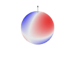
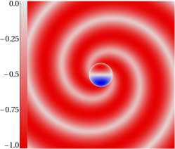
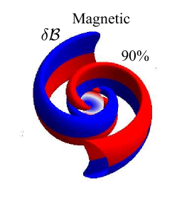
Figure 19: (color online). The $(2,1)$ magnetic-parity horizon vorticity and vortexes. Left panel: The horizon vorticity for the $(2,1)$ magnetic-parity perturbation of Schwarzschild, colored as in Fig. 9. There are four horizon vortexes, two clockwise (blue [dark gray]) and two counterclockwise (red [light gray]). The horizon vorticity vanishes at the equator and the poles. Middle panel: Vorticity of the counterclockwise vortex lines passing through the equatorial plane, colored and normalized as in the middle and right hand columns of Fig. 10 and plotted in a region $24M$ across. The (blue [dark gray]) vorticity of the clockwise vortex lines has precisely this same pattern, because the two families of lines pass through the equatorial plane with the same magnitude of vorticity at each point. Right panel: Three dimensional vortexes colored and labeled as in Fig. 14. By near duality, this figure also represents (to good accuracy) the tendicity and tendex structure of the (2,1) electric-parity mode.

The horizon vorticity of the magnetic-parity (2,1) mode has an angular dependence given by the spherical harmonic $Y^{21}(\theta,\phi)$ (of course). We display this horizon vorticity in the left panel of Fig. 19. There are four horizon vortexes, two of each sign, and vanishing horizon vorticity all along the equator.

As we noted in Sec. I.3.7, this mode’s symmetry dictates that the frame-drag field be reflection antisymmetric through the equatorial plane. As for the electric-parity (2,2) frame drag field, which also has this property (second paragraph of Sec. III.2; also Sec.  III.2.4 and Fig. 13), this implies that one family of vortex lines lies in the equatorial plane with vanishing vorticity, and two cross through that plane at $45^{\circ}$ with equal and opposite vorticities. The negative vorticities of the crossing lines are plotted in the middle panel of Fig. 19, along with the projected horizon vorticity, as if the horizon were viewed from above. The positive-vorticity pattern of the other family of crossing lines is identical to this negative-vorticity pattern, since at each point the two lines have the same vorticity magnitude.

The fact that there are just two spiraling vortexes in this figure, by contrast with four for the (2,2) modes, is guaranteed by the modes’ azimuthal orders, $m=1$ here and $m=2$ for (2,2).

The vortex structure outside the equatorial plane, depicted in the right panel of Fig. 19, was discussed in Sec. I.3.7. The two red (light gray), 3D vortexes are the same ones depicted in the middle panel. They actually extend across the equatorial plane (via the $45^{\circ}$ vortex lines) into the region occupied by the blue (dark gray) vortexes; but we do not see them there in the 3D drawing because the blue vortexes have larger vorticity and we have chosen to show at each point only the largest-vorticity vortex.

V.2 Vortexes of $(2,1)$ electric-parity mode and perturbative tendexes of $(2,1)$ magnetic-parity mode

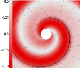
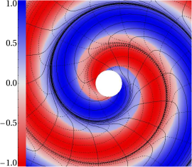
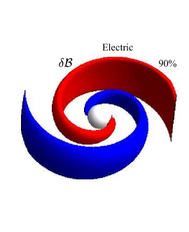
Figure 20: (color online). The $(2,1)$ electric-parity vortex lines, vorticities and vortexes in the equatorial plane. For this mode the horizon’s vorticity vanishes, so the horizon is plotted as a white disk or sphere. Left panel: Counterclockwise vortex lines (dashed) and their vorticity (red [light gray] color) normalized as in Fig. 10, and plotted in a region $24M$ across. Middle panel: Both clockwise (solid) and counterclockwise (dashed) vortex lines, and the vorticity (color) of the line with the larger magnitude of vorticity, in a region $24M$ across. Right Panel: Three-dimensional vortexes colored and labeled as in Fig. 14. By near duality, this figure also represents to good accuracy the perturbative tendex lines, tendicities and tendexes for the magnetic-parity (2,1) mode.

Turn, next, to the vortex lines and vortex structure of the (2,1) electric-parity mode. [By near duality, the perturbative tendex lines and tendex structure of the (2,1) magnetic-parity mode will be the same.]

For this mode, with the parity reversed from the previous section, the frame-drag field is symmetric under reflection through the equatorial plane rather than antisymmetric. Therefore, there are two sets of vortex lines that remain in the equatorial plane, with the third set normal to it. In this sense the vortexes structures are analogous to those of the magnetic-parity, $(2,2)$ mode; and in fact they are strikingly similar, aside from having two arms rather than four.

We show the vortexes and vortex lines in Fig. 20. The left and middle panels of Fig. 20 show the lines that remain in the equatorial plane, along with color-intensity plots depicting the lines’ vorticities.

The left panel of Fig. 20 shows the counterclockwise lines and their vorticities. As in the case of the $(2,2)$ mode, we see a spiraling region of strong vorticity which contacts the horizon, and an accompanying spiral of low vorticity. At the horizon, the frame-drag field is primarily longitudinal-transverse, and correspondingly its vortex lines enter the horizon at a (nearly) $45^{\circ}$ angle. As for the (2,2) mode, there is a limiting spiral that all the outspiraling vortex lines approach, near the edge of the vortex.

There is also a small region of strong vorticity near the horizon which forms a second spiral, opposite the primary spiral, although it quickly becomes weak; this second vortex coincides with the region of strong positive vorticity, as we see in the middle panel of Fig. 20, and we think its existence is due to the frame-drag field at the horizon being primarily longitudinal-transverse. It also should be compared to the similar regions of strong negative vorticity near the positive horizon vortexes of the magnetic-parity $(2,2)$ mode in Fig. 10.

In the middle panel, we plot both the counterclockwise (dashed) and clockwise (solid) vortex lines, and we color each point by the vorticity that is strongest. We see two strong vortexes spiraling out to form gravitational waves, and we see that under a rotation through $180^{\circ}$ the clockwise and counterclockwise vortex lines map into each other.

Finally, in the right panel of Fig. 20, we show the vortexes in three dimensions using the same conventions as in Fig. 14: the red (light gray) and blue (dark gray) surfaces are the locations where the vorticity of largest magnitude has fallen to $90\%$ of its maximum at each radius. By contrast with the (2,1) magnetic-parity mode, where the 3D vortexes are antisymmetric through the equator (and so they flip colors; see Fig. 19), here they are symmetric and so have the same color above and below the equatorial plane.

By duality, for the (2,1) magnetic-parity mode, with its antisymmetric 3D vortexes (Fig. 19), the 3D perturbative tendexes are symmetric through the equatorial plane and have the form shown in this right panel of Fig.  20.

V.3 Vortexes of $(2,0)$ magnetic-parity mode and perturbative tendexes of (2,0) electric-parity mode

In Sec. I.3.8, we described in detail the dynamics of the axisymmetric (2,0) magnetic-parity mode of Schwarzschild and the gravitational waves it emits—waves in which the vortex and tendex lines wrap around deformed tori. In this section and the next, we shall discuss some other details of this mode and its dual, the (2,0) electric-parity mode.

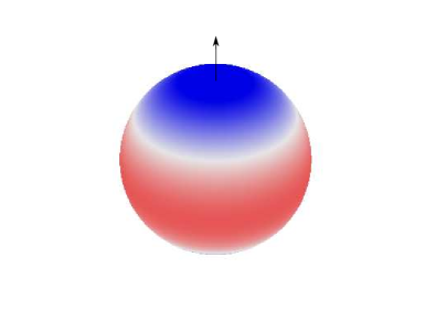
Figure 21: (color online). The horizon vorticities $(\delta\mathcal{B}_{NN})$ of the quadrupolar, $(2,0)$, magnetic-parity mode. As in Fig. 9, the color intensity is proportional to the magnitude of the vorticity with blue (dark gray) for positive and red (light gray) for negative. The arrow points along the polar axis. The vorticity oscillates sinusoidally in time, causing $\delta\mathcal{B}_{NN}$ first to vanish and then to change sign.

In Fig. 21, we show the horizon vorticity for this magnetic-parity mode. Of course, it is proportional to the scalar spherical harmonic $Y^{20}(\theta,\phi)$. At this moment of time, there are clockwise vortexes (blue [dark gray]) in the northern and southern hemispheres, and a band-shaped counterclockwise vortex (red [light gray]) in the equatorial region. As time passes, the horizon vorticity oscillates, with red vortexes becoming blue and blue becoming red in each half cycle, while also decaying exponentially. The cause of these oscillations, as we discussed in Sec. I.3.8, is exchange of energy between $\delta{\bm{\mathcal{B}}}^{\rm L}$ (whose normal-normal component is the horizon vorticity) and $\delta{\bm{\mathcal{E}}}^{\rm LT}$ (which we will visualize in the next section).

As we discussed in Sec. I.3.8, symmetries dictate that this mode have two families of vortex lines lying in planes $\mathcal{S}_{\phi}$ of constant $\phi$ and a third family consisting of azimuthal circles of constant $r$ and $\theta$. In Fig. 6, we explored in detail the wave-zone wrap-around-torus shapes of the $\mathcal{S}_{\phi}$ vortex lines, and their vorticity patterns. In the near zone, the line shapes and vorticities are somewhat more complex. We elucidate them in Fig. 22, where, to make the figure more understandable and preserve some features lost in Fig. 6, we show the two families of vortex lines in separate panels, left and center.

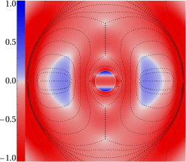
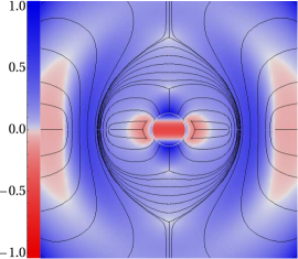
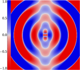
Figure 22: (color online). Left and middle panels: Near- and transition-zone vortex lines and their vorticities in an $\mathcal{S}_{\phi}$ plane of constant $\phi$, for the axisymmetric (2,0) magnetic-parity mode of Schwarzschild in the near and transition zones ($30M$ across). Left panel: The predominantly counterclockwise family of vortex lines. Middle panel: The predominantly clockwise family of vortex lines. Right panel: Vorticity of the axial lines normal to an $\mathcal{S}_{\phi}$ plane, in near and wave zones ($56M$ across). The color intensity in each panel gives the vorticity of the lines, scaled as in Fig. 16.

As for the superposed $(2,2)$ and $(2,-2)$ perturbations of Sec. IV, each family takes on both positive and negative vorticities, but is predominantly one or the other. And unlike the (2,2) mode and the superposed mode, the (2,0) line families do not map into each other after a $90^{\circ}$ rotation; rather, they have distinct patterns (as one might expect, since their plane is $\mathcal{S}_{\phi}$ rather than the equatorial plane). On the other hand, because of this mode’s oscillating nature, the predominantly positive lines are the same as the predominantly negative lines a half-cycle previous (with signs reversed). For this reason, we illustrate the two families at the same moment in time, the moment when the horizon vorticity reaches a maximum with blue (dark gray) near the poles and red (light gray) near the equator.

One striking feature of Fig. 22 is a set of isolated points where six lines meet, three from each family (three in each panel). These are nodes (zeros) of the frame-drag field, as one can see from the fact that the coloring there is white. These are also points where, dynamically, the field lines can reconnect, changing their topologies.

Let us focus on the near-horizon, predominantly negative vortex lines (dashed lines) in the left panel of Fig. 22. The lines that emerge from the counterclockwise horizon vortex in the equatorial region loop over the north or south pole of the black hole, and reconnect to the opposite side of that horizon vortex. We think that, as the mode oscillates, these lines will merge at the equator then slide off the horizon and form closed loops surrounding the hole, of the sort that we see in the outer parts of the lenticular blue (dark gray) region of the center panel, and these will then expand and deform and reconnect to form the set of wrap-around-deformed-torus lines of the left panel, which lie in the outer part of the transition zone and are becoming outgoing gravitational waves.

Next focus on the near-horizon, predominantly positive vortex lines (solid lines) in the middle panel of Fig. 22. The lines, that emerge from the clockwise horizon vortex in the north polar region, swing around the equator and descend into the south polar horizon vortex. We think that, as the oscillation proceeds, these lines will slide off the horizon and immediately form closed loops that wrap around deformed tori, which expand to become like those near the left and right edges of the left panel (outer part of transition zone), and then continue their expansion, becoming the gravitational-wave wrap-around-torus lines whose inner parts are at the left and right edges of the right panel.

Notice, in the middle panel near the equator, two regions of weakly negative (pink [light gray]) vorticity, and their near-zone lines that appear to have just disconnected from the horizon but are mostly radially directed. And notice similarly the pink regions near the left and right edges of this panel, again with vortex lines that are traveling roughly radially. These pink regions are actually toroidal, because of the rotation symmetry around the vertical axis. In the outer transition zone and the wave zone, they are the regions in which this family’s wrap-around-torus, gravitational-wave vortex lines are crossing over from one clockwise vortex (wave crest) to another. This feature of crossover lines with weakly reversed vorticity appears to be a robust feature of oscillatory modes. For other examples, see the weakly blue regions in the left panel, and see the superposed (2,2) and (2,-2) mode in Fig. 16, where the dashed vortex lines, with predominantly counterclockwise (red [light gray]) vorticity, become weakly blue (darker gray) in the crossover regions.

The right panel of Fig 22 shows the vorticity of the axial lines (constant $r,\theta$ circles) in both near zone and wave zone. Near the horizon, these lines are largely part of the transverse, isotropic piece of the longitudinal field $\delta{\bm{\mathcal{B}}}^{\rm L}$; they have opposite color to the horizon vortexes at the horizon, as they must, in order to keep $\delta{\bm{\mathcal{B}}}^{\rm L}$ trace-free. Near the horizon, these lines also contain a smaller component of the ingoing-wave transverse-traceless field $\delta{\bm{\mathcal{B}}}^{\rm TT}$. In the wave zone, they are fully outgoing-wave $\delta{\bm{\mathcal{B}}}^{\rm TT}$.

V.4 Vortex lines of $(2,0)$ electric-parity mode and perturbative tendex lines of (2,0) magnetic-parity mode

For the (2,0) electric-parity mode of Schwarzschild in RWZ gauge, the only nonzero components of the frame-drag field are $\delta\mathcal{B}_{\hat{r}\hat{\phi}}$ and $\delta\mathcal{B}_{\hat{\theta}\hat{\phi}}$. Near the horizon, where decomposition into longitudinal, longitudinal-transverse, and transverse-traceless parts is meaningful, $\delta\bm{\mathcal{B}}^{\rm L}$ vanishes (and hence the horizon vorticity vanishes), $\delta\mathcal{B}_{\hat{r}\hat{\phi}}$ is the sole component of $\delta\bm{\mathcal{B}}^{\rm LT}$, and $\delta\mathcal{B}_{\hat{\theta}\hat{\phi}}$ is the sole component of $\delta\bm{\mathcal{B}}^{\rm TT}$.

By (near) duality, the same is true for the (2,0) magnetic-parity mode of the last subsection, with $\delta\bm{\mathcal{B}}$ replaced by $\delta\bm{\mathcal{E}}$.

Because the only nonzero components are $\delta\mathcal{B}_{\hat{r}\hat{\phi}}$ and $\delta\mathcal{B}_{\hat{\theta}\hat{\phi}}$ and because of the axisymmetry, there is a family of zero-vorticity vortex lines which lie in a plane $\mathcal{S}_{\phi}$ of constant $\phi$, and the other two sets of vortex lines have equal and opposite vorticity and pass through $\mathcal{S}_{\phi}$ at 45 degree angles. In Fig. 23, we show in $\mathcal{S}_{\phi}$ the vorticity of the counterclockwise lines that pass through it. A plot for the clockwise lines would be identical, but with blue changed into red.

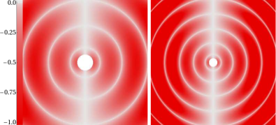
Figure 23: (color online). For the (2,0) electric-parity mode of Schwarzschild in RWZ gauge: the vorticity of the counterclockwise vortex lines that pass through the plane $\mathcal{S}_{\phi}$ of constant $\phi$. The color intensity (scale on left) is scaled as in Fig. 16. Left panel: $30M$ across, showing the near and intermediate zones and beginning of the wave zone. Right panel: $56M$ across.

Notice the remarkable absence of structure in the near zone. All we see is toroidal vortexes separated by circular null surfaces and a polar null line. (Recall the axisymmetry around the vertical polar axis). The absence of structure is presumably due to the fact that this mode is sourced by the longitudinal perturbative tendex field, and not by this frame-drag field (though its longitudinal-transverse part plays a key role of periodically storing near-zone energy during the oscillations; cf. the discussion of the dual mode below). The vorticity vanishes along the polar axis because of axisymmetry and the fact that the radial-radial part of the frame-drag field vanishes.

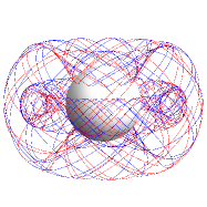
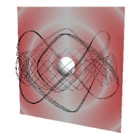
Figure 24: (color online). Vortex lines for the $(2,0)$ electric-parity mode of Schwarzschild in RWZ gauge. Left panel: Two vortex lines of each sign in the near zone and innermost part of transition zone. The positive (blue lines) and negative (red) lines are identical but wind their tori in opposite directions. Right panel: Two counterclockwise vortex lines in the transition zone, with the vorticity shown in a semitransparent slice $\mathcal{S}_{\phi}$ of constant $\phi$ as a density plot. The vortex lines are plotted in black rather than red in this panel to aid the eye.

For greater insight into this frame-drag field, we show in the left panel of Fig. 24 several of its three-dimensional vortex lines in the near zone and innermost part of the transition zone. These vortex lines wind densely around axisymmetric deformed tori.

Note that the large torus is attached to the horizon. Its vortex lines intersect the horizon at the approximately $45^{\circ}$ angles characteristic of the longitudinal-transverse part of the field, which is these lines’ dominant component.

For the dual, magnetic-parity (2,0) mode, this torus depicts the perturbative tendex lines of the near zone, and those lines predominantly belong to the longitudinal-transverse part of the tidal field, $\delta\bm{\mathcal{E}}^{\rm LT}$. This is the part that stores the mode’s near-zone oscillation energy when $\delta\bm{\mathcal{B}}^{\rm L}$ is passing through zero and its perturbative vortex lines are detached from the horizon (see the discussion of this mode’s dynamics in Sec. I.3.8). Immediately after this snapshot, these tendex lines’ $\delta\bm{\mathcal{E}}^{\rm LT}$ begin to regenerate the near-horizon longitudinal frame-drag field $\delta\bm{\mathcal{B}}^{\rm L}$ and its horizon vorticity. As it does so, these tendex lines and their torus (presumably) detach from the horizon and expand outward into the transition then wave zone, becoming the tendex-line component of a gravitational-wave torus like those displayed in Fig. 7 above.

The small torus in the left panel of Fig. 24 encircles the equatorial point on the innermost node of the field (innermost white circle in Fig. 23). It is also the innermost torus shown in Fig. 7 above.

In the right-hand panel of Fig. 24, for the (2,0) electric-parity mode we show two counterclockwise vortex lines in the transition zone. By chance, the larger of the selected lines nearly forms closed orbits, and so even after wrapping its torus four times it appears as a thin ribbon. While it is difficult to tell with this nearly closed line, extended integration reveals that it does wrap a (deformed) torus.

Notice that both lines (both tori) in the right panel straddle the second null of the frame-drag field (second-from-center white circle in Fig. 23).

VI Conclusions

Although the theory of black-hole quasinormal modes is roughly half a century old, most past studies of them have focused on their mathematical properties, their eigenfrequencies and emitted gravitational waves, and their excitation by various physical processes. Aside from a geometric-optics interpretation of high-frequency modes (see, e.g., Ferrari and Mashhoon (1984); Dolan (2010); Yang et al. (2012)), little was known, before this paper, about their geometrodynamic properties—e.g., the structure and dynamics of their spacetime curvature in the near zone and transition zone, and how the near-zone curvature generates gravitational waves.

In this paper we have used our new vortex and tendex tools to explore, in depth, the geometrodynamics of the quadrupolar modes for Schwarzschild and Kerr black holes. Most importantly, we have discovered that:

(i) There is a near duality between electric-parity modes and magnetic-parity modes, in which tendexes get mapped into vortexes and vortexes into tendexes.

(ii) The electric-parity $(l,m)=(2,2)$ and (2,1) modes are generated by near-zone, longitudinal vortexes that extend out of the horizon and rotate (four tendexes for $m=2$; two for $m=1$). The vortexes’ rotation generates outgoing and ingoing gravitational waves; the ingoing waves act back on the longitudinal vortexes, gradually pushing them off the horizon, which results in the mode’s exponential attenuation.

(iv) By (near) duality, the electric-parity (2,2) and (2,1) modes are generated and attenuated in the same way, but with near-zone, longitudinal tendexes rather than vortexes playing the central role.

(v) The magnetic-parity (2,0) mode and superposed (2,2) & (2,-2) mode are generated by near-zone, longitudinal vortexes that extend out of the horizon and oscillate between clockwise and counterclockwise vorticity. In these oscillations, energy is fed back and forth between the longitudinal vortexes and longitudinal-transverse, near-zone tendexes that do not penetrate the horizon. In each oscillation, as the horizon vorticity passes through zero, the longitudinal vortex lines slide off the horizon and reconnect to form toroidal vortexes that travel outward, becoming gravitational waves; and the near-zone tendexes then regenerate the longitudinal vortexes (with reversed vorticity), thereby triggering the next half cycle of oscillation.

(vi) The electric-parity (2,0) mode and superposed (2,2) & (2,-2) mode exhibit these same geometrodynamics, but with the roles of the vortexes and tendexes reversed.

In future papers, these quasinormal-mode insights will be a foundation as we explore the geometrodynamics of merging binary black holes using numerical simulations.

While all analytic approximations fail near the time of merger, black-hole perturbation theory does approximate a binary-black-hole spacetime well in some epochs: the merged hole during its ringdown, each tidally deformed hole during inspiral, and each perturbed hole during the initial relaxation that causes spurious “junk” gravitational radiation. Before exploring the fully nonlinear vortex and tendex structures in simulations, we are likely first to compare numerical vortex and tendex structures during these epochs with the corresponding perturbative results (as in Fig. 15). Such comparisons will allow us to determine to what degree the insights we have gained from our perturbative studies can also be applied to numerical simulations—particularly the relative insensitivity of vortexes and tendexes to changes in gauge and slicing.

Building on these comparisons, our future work will then include initial explorations of the fully nonlinear geometrodynamics of the warped spacetimes present in binary-black-hole simulations. For example, Kamaretsos, Hannam, and Sathyaprakash Kamaretsos et al. (2012) have recently observed relationships between the properties (masses and spins) of the initial holes in a binary-black-hole merger and the particular quasinormal modes that are excited in the remnant (modes which generate the ringdown portion of the gravitational waves). By examining the vortex and tendex structures of a variety of binary-black-hole mergers, we hope to gain insight into the origin of such relationships. Also, following Dennison and Baumgarte’s recent exploration Dennison and Baumgarte (2012) of the vortex and tendex structures in approximate, perturbative initial data, we intend to explore the vortex and tendex structures of constraint-satisfying binary-black-hole initial data, which could give insight into the initial perturbations (and the corresponding spurious “junk” gravitational radiation) that appear in all currently used, binary-black-hole initial-data schemes.

Ultimately, we plan to use vortexes and tendexes to explore the geometrodynamics of binary-black-hole spacetimes throughout the entire simulated inspiral, merger, and ringdown. We expect that these tools will provide insights into the behavior of these spacetimes and perhaps also motivate new ways of constructing phenomenological waveform templates for use in gravitational-wave data analysis.

Appendix A Quasinormal Modes of a Schwarzschild Black Hole in Regge-Wheeler Gauge

In this appendix, we review the Regge-Wheeler-Zerilli (RWZ) formalism for black-hole perturbations, and we discuss the calculations that underlie the results reported in Secs. III, IV, and V for quadrupolar perturbations of non-spinning black holes in the RWZ gauge.

A.1 Regge-Wheeler-Zerilli formalism

Here we review the equations governing quasinormal modes for a non-rotating black hole in the Regge-Wheeler-Zerilli gauge Regge and Wheeler (1957); Zerilli (1970). We write the metric in Schwarzschild coordinates with a small perturbation $h_{\mu\nu}$,

$$ds^{2} = -\alpha^{2}dt^{2}+\frac{dr^{2}}{\alpha^{2}}+r^{2}(d\theta^{2}+\sin^{2}\theta d\phi^{2})+h_{\mu\nu}dx^{\mu}dx^{\nu}\>,$$

$$\alpha^{2} = 1-2M/r\>.$$ (29)

The components of $h_{\mu\nu}$ obey separable differential equations, and importantly $h_{\mu\nu}$ can be split into definite-parity perturbations (electric and magnetic) which do not couple to each other.

For magnetic-parity perturbations, the only nonzero components of $h_{\mu\nu}$ in Regge-Wheeler gauge are

$$h_{tA}=h_{0}(r)e^{-i\omega t}X^{lm}_{A}(\theta,\phi)\;,\quad h_{rA}=h_{1}(r)e^{-i\omega t}X^{lm}_{A}(\theta,\phi)\;.$$ (30)

Here $\omega$ is the mode’s complex QNM eigenfrequency, and $X^{lm}_{A}$ is the magnetic-parity vector spherical harmonic on the unit two-sphere,

$$X^{lm}_{\theta}=-\csc\theta\,{Y^{lm}}_{,\phi}\;,\qquad X^{lm}_{\phi}=\sin\theta\,{Y^{lm}}_{,\theta}\;,$$ (31)

with $Y^{lm}(\theta,\phi)$ denoting the scalar spherical harmonics. Regge and Wheeler Regge and Wheeler (1957); Edelstein and Vishveshwara (1970) showed that the radial parts of the metric perturbation, $h_{0}(r)$ and $h_{1}(r)$, can be expressed in terms of a single scalar radial eigenfunction $Q(r)$ as

$$h_{0}=-\frac{\alpha^{2}}{i\omega}(rQ)_{,r}\;,\quad h_{1}=\frac{rQ}{\alpha^{2}}\;,$$ (32)

which satisfies the eigenequation

$$Q_{,r_{*}r_{*}}+\omega^{2}Q=\mathcal{V}_{Q}(r)Q\;,\;\;\mathcal{V}_{Q}(r)=\alpha^{2}\left(\frac{l(l+1)}{r^{2}}-\frac{6M}{r^{3}}\right)\;.$$ (33)

Here $r_{*}$ is the tortoise coordinate

$$dr_{*}=\frac{dr}{\alpha^{2}}\;,\quad r_{*}=r+2M\ln(\alpha^{2}r/2M)\;,$$ (34)

which goes to $+\infty$ far from the hole and $-\infty$ at the hole’s horizon. This eigenequation must be solved subject to the boundary conditions of outgoing waves at infinity, $Q\sim e^{i\omega r_{*}}$ as $r_{*}\rightarrow+\infty$, and ingoing waves at the horizon, $Q\sim e^{-i\omega r_{*}}$ as $r_{*}\rightarrow-\infty$.

For electric-parity modes, the nonzero components of $h_{\mu\nu}$ in RWZ gauge are Zerilli (1970)

$$h_{tt}=\alpha^{2}H_{0}(r)e^{-i\omega t}Y^{lm}\;, h_{rr}=\frac{H_{0}(r)}{\alpha^{2}}e^{-i\omega t}Y^{lm}\;,$$

$$h_{tr}=H_{1}(r)e^{-i\omega t}Y^{lm}\;, h_{AB}=r^{2}\Omega_{AB}K(r)e^{-i\omega t}Y^{lm}\;.$$

Here $\Omega_{AB}$ denotes the metric on the unit 2-sphere. We can write the metric perturbation functions in terms of the Zerilli function $Z(r)$ as

$$K = \left[\frac{\lambda(\lambda+1)r^{2}+3\lambda Mr+6M^{2}}{r^{2}(\lambda r+3M)}\right]Z+\alpha Z_{,r}\;,$$

$$H_{1} = -i\omega\left[\frac{\lambda r^{2}-3\lambda Mr-3M^{2}}{(r-2M)(\lambda r+3M)}\right]Z-i\omega rZ_{,r}\;,$$

$$H_{0} = \left[\frac{\lambda r(r-2M)-\omega^{2}r^{4}+M(r-3M)}{(r-2M)(\lambda r+3M)}\right]K$$ (36)

$$+\left[\frac{(\lambda+1)M-\omega^{2}r^{3}}{i\omega r(\lambda r+3M)}\right]H_{1}\;.$$

Here we have used Zerilli’s notation

$$\lambda=\frac{1}{2}(l-1)(l+2)\;.$$ (37)

The Zerilli function satisfies the eigenequation

$$Z_{,r_{*}r_{*}}+\omega^{2}Z=\mathcal{V}_{z}(r)Z\;,$$ (38)

where

$$\mathcal{V}_{z}(r)=\alpha^{2}\left[\frac{2\lambda^{2}(\lambda+1)r^{3}+6\lambda^{2}Mr^{2}+18\lambda M^{2}r+18M^{3}}{r^{3}(\lambda r+3M)^{2}}\right].$$ (39)

The slices of constant Schwarzschild time $t$ do not intersect the black hole’s horizon, so in performing our 3+1 split, we use slices of constant Eddington-Finklestein time $\tilde{t}=t+2M\ln(r/2M-1)$. Written in Schwarzschild coordinates, the perturbed tetrad for the EF observers is given by Eqs. (8) and  (11). For any chosen mode, we compute the frame-drag and tidal fields by (i) computing, from the metric-perturbation components $h_{\mu\nu}$, the perturbation $\delta R_{\alpha\beta\gamma\delta}$ to the Riemann tensor (same as Weyl) in Schwarzschild coordinates; (ii) projecting the total Riemann tensor $R_{\alpha\beta\gamma\delta}=R^{(0)}_{\alpha\beta\gamma\delta}+\delta R_{\alpha\beta\gamma\delta}$ (where $R^{(0)}_{\alpha\beta\gamma\delta}$ is the unperturbed Riemann tensor) onto the perturbed EF tetrad; (iii) reading off $\mathcal{E}_{\hat{a}\hat{b}}=R_{\hat{a}\hat{0}\hat{b}\hat{0}}$ and $\mathcal{B}_{\hat{a}\hat{b}}=\tfrac{1}{2}\epsilon_{\hat{a}\hat{p}\hat{q}}R_{\hat{p}\hat{q}\hat{0}\hat{b}}$ and splitting them into their unperturbed and perturbed parts.

A.2 Magnetic-parity $(2,m)$ mode: Frame-drag field

We first focus on the $(2,m)$ quadrupolar modes for magnetic-parity perturbations. Carrying out the above computation, expressing the answer for the frame-drag field in terms of the Regge-Wheeler function $Q(r)$ and the electric-parity scalar, vector, and tensor harmonics (see discussion in App. C.3), and simplifying using Eq. (33), we obtain:

$$\mathcal{B}^{(1)}_{\hat{r}\hat{r}} =\Re\left[B_{1(\rm{m})}e^{-i\omega t}Y^{2m}\right]\;,$$ (40a)

$$\mathcal{B}^{(1)}_{\hat{r}\hat{A}} =\Re\left[B_{2(\rm{m})}e^{-i\omega t}Y^{2m}_{\hat{A}}\right]\;,$$ (40b)

$$\mathcal{B}^{(1)}_{\hat{A}\hat{B}} =\Re\left[\left(-\frac{1}{2}B_{1(\rm{m})}\delta_{\hat{A}\hat{B}}Y^{2m}+B_{3(\rm{m})}Y^{2m}_{\hat{A}\hat{B}}\right)e^{-i\omega t}\right],$$ (40c)

$$B_{1(\rm{m})}(r) =-\frac{12Q}{i\omega r^{3}}\>,$$ (40d)

$$B_{2(\rm{m})}(r) =-\frac{4iM\omega Q+2\alpha^{2}rQ^{\prime}}{i\omega r^{3}\alpha^{2}\sqrt{1+2M/r}}\,,$$ (40e)

$$B_{3(\rm{m})}(r)=-\frac{1}{i\omega r^{5}\alpha^{4}(r+2M)}\Big{(} \left[3\alpha^{2}(r-M)(r^{2}+4M^{2})+4iM\omega r^{2}(r-3M)-r^{3}\omega^{2}(r^{2}+4M^{2})\right]Q$$

$$+r\alpha^{2}\left[(r-3M)(r^{2}+4M^{2})+4iM\omega r^{3}\right]Q^{\prime}\Big{)}\;,$$ (40f)

where a prime denotes a derivative with respect to $r$, $Y^{lm}_{A}$ and $Y^{lm}_{AB}$ are given by Eqs. (84), and $\delta_{\hat{A}\hat{B}}$ is the Kronecker delta.

We have solved the Regge-Wheeler equation (33) numerically for the most slowly damped, quadrupolar normal mode. When the numerical solution is inserted into the above expressions for $\mathcal{B}^{(1)}_{\hat{a}\hat{b}}$, numerical errors cause problems with delicate cancellations in the transverse-traceless and radial-transverse components near the horizon. To deal with this, we have derived the following asymptotic formula for $Q(r)$ near the horizon, $r_{*}/M\ll-1$:

$$Q = Y^{-2iM\omega}\left[1+\frac{3Y}{(1-4iM\omega)e}\right.$$

$$+\frac{9iM\omega Y^{2}}{(1-4iM\omega)(1-2iM\omega)e^{2}}$$

$$\left.-\frac{3(1+12iM\omega+40M^{2}\omega^{2})Y^{3}}{2(1-4iM\omega)(1-2Mi\omega)(3-4iM\omega)e^{3}}+O(Y^{4})\right]\;$$

where $Y=e^{r_{*}/2M}$. Inserting this into Eqs. (40), we find, of course, that all components of $\mathcal{B}_{\hat{a}\hat{b}}$ are finite at the horizon.

Using Eqs. (40) for the frame-drag field, our analytic formula (LABEL:Qanalytic) for $Q(r)$ near the horizon, and our numerical solution for $Q(r)$ at larger radii, and the $(2,2)$ harmonics, we compute the vortex lines and their vorticities for the fundamental $(2,2)$ quasinormal mode. We illustrate them in Figs. 2, 3, 4 and 10.

For our superposition of the $(2,2)$ and $(2,-2)$ modes we can simply sum the $(2,2)$ and $(2,-2)$ harmonics in the above expressions. We plot the vortex lines for the resulting frame-drag field in Figs. 8, 16, and the top row of Fig. 18. We use the $(2,1)$ harmonics for generating the vortexes of the magnetic-parity, $(2,1)$ perturbations that are illustrated in Fig. 19. Finally, we use the $(2,0)$ harmonics to produce the vortexes and vortex lines of the $(2,0)$ magnetic-parity perturbation. We note that $Y^{20}_{\hat{\phi}}=Y^{20}_{\hat{\theta}\hat{\phi}}=0$ for this mode. This means that $\mathcal{B}^{(1)}_{\hat{a}\hat{b}}$ is block-diagonal, and the vortex lines split into a pair of lines which remains in a slice of constant $\phi$ and a single, axial line that runs in circles of constant $(r,\theta)$. In a slice of constant $\phi$, we illustrate the two sets of vortex lines in the slice and their voticity together in Fig. 6 and separately in the left and middle panels of Fig. 22. We also plot the vorticity of the axial lines in a slice in the right panel of Fig. 22.

A.3 Electric-parity $(2,m)$ modes: Frame-drag field

Carrying out the calculation described at the end of Sec. A.1 using the electric-parity metric perturbation (LABEL:EPmetric), expressing the result in terms of the Zerilli function $Z$ with the aid of Eqs. (36), and simplifying using Zerilli’s differential equation (38), we obtain for the frame-drag field of a $(2,m)$ electric-parity perturbation

$$\mathcal{B}^{(1)}_{\hat{r}\hat{r}} =0\,,$$ (42a)

$$\mathcal{B}^{(1)}_{\hat{r}\hat{A}} =\Re\left[B_{1(\rm{e})}e^{-i\omega t}X^{2m}_{\hat{A}}\right]\,,$$ (42b)

$$\mathcal{B}^{(1)}_{\hat{A}\hat{B}} =\Re\left[B_{2(\rm{e})}e^{-i\omega t}X^{2m}_{\hat{A}\hat{B}}\right]\,,$$ (42c)

where

$$B_{1(\rm{e})}= \frac{\left[6M^{2}\alpha^{2}-i\omega r^{2}(2r+3M)\right]Z-2Mr\alpha^{2}(2r+3M)Z^{\prime}}{2r^{5}\alpha^{2}\sqrt{1+2M/r}}\,,$$ (42d)

$$B_{2(\rm{e})}= \frac{1}{2r^{4}\alpha^{4}(2r+3M)(r+2M)}\Big{(}\left[-12M\alpha^{2}(M^{2}+4r\beta_{1})-i\omega(r^{2}+4M^{2})\beta_{2}+4M\omega^{2}r^{3}(2r+3M)\right]Z$$

$$\qquad\qquad\qquad\qquad\qquad\qquad-r\alpha^{2}\left[4M\beta_{2}+i\omega r(2r+3M)(r^{2}+4M^{2})\right]Z^{\prime}\Big{)}\,.$$ (42e)

Here a prime denotes a derivative with respect to $$r X^{lm}_{A} X^{lm}_{AB}$$, and and are the magnetic-parity vector and tensor spherical harmonics given by Eqs. (87) (see discussion in App. C.3). We have defined here for convenience the functions

$$\beta_{1} =\frac{r^{2}+Mr+M^{2}}{2r+3M}\,, \beta_{2} =(2r^{2}-6Mr-3M^{2})\,.$$ (42f)

We note again that the horizon vorticity, $\mathcal{B}^{(1)}_{NN}$, vanishes. With this $\mathcal{B}^{(1)}_{\hat{a}\hat{b}}$ we can again compute the eigenvector fields and eigenvalues for the perturbed spacetime, and from them compute the vortex lines. We use these expressions to calculate the vortex lines and their vorticities generated by electric-parity perturbations. In order to compute the vortex lines for these modes, once again we expand $Z$ around the horizon in terms of $Y=e^{r_{*}/2M}$ up to $O(Y^{3})$. We use this series to match to a numerical solution of the Zerilli equation subject to ingoing-wave boundary conditions. Because the Zerilli potential $\mathcal{V}_{z}$ is more complicated than the Regge-Wheeler potential $\mathcal{V}_{Q}$, the coefficients of the expansion of $Z$ in powers of $Y$ are lengthy, but easily computed using algebraic computing software such as Mathematica. For this reason, we do not give the coefficients here.

For an electric-parity $(2,2)$ perturbation, the only set of vortex lines that are confined to the equatorial plane have vanishing vorticity (and are of less physical interest). Instead, we used the above frame-drag field to compute, and then plot in Fig. 13, the vorticity of one of the sets of vortex lines that pass through the equatorial plane at a 45 degree angle: the set with negative vorticity. Just as with the magnetic-parity modes, we superpose a $(2,2)$ perturbation with a $(2,-2)$ perturbation by a simple sum of the harmonics. The vorticity of these lines passing through the equatorial plane (the analog of Fig. 13) is plotted in Fig. 17.

For the vortex lines of the $(2,1)$ mode, there is a reflection symmetry about the equatorial plane, which implies that there are two sets of vortex lines confined to the plane, with a third normal to it. We illustrate the vortex lines and 3D vortexes of this mode in Fig. 20. Finally, when we use the $(2,0)$ harmonics, we note that $X^{20}_{\hat{\theta}}=X^{20}_{\hat{\theta}\hat{\theta}}=X^{20}_{\hat{\phi}\hat{\phi}}=0$. While this means that the frame drag field is simple, it is not block-diagonal and its nonzero vortex lines pass through all three dimensions. There is a single set of axial vortex lines with zero vorticity, and two sets with equal and opposite vorticity that wind around deformed tori. We illustrate the vorticity in a slice of constant $\phi$ for the negative lines in Fig. 23. In addition, we illustrate some 3D vortex lines in Figs. 7 and 24.

A.4 Electric-parity $(2,2)$ mode: Tidal field

To help understand the slicing dependence of our results, we compare fields generated by electric-parity perturbations, because the slicings are identical for all magnetic-parity perturbations. In particular, we focused on the perturbed tidal field for the electric-parity, $(2,2)$ mode. Carrying out the calculation of this mode as above when using the electric-parity metric perturbation (LABEL:EPmetric), we obtain

$$\mathcal{E}^{(1)}_{\hat{r}\hat{r}} =\Re\left[E_{1(\rm{e})}e^{-i\omega t}Y^{22}\right]\,$$ (43a)

$$\mathcal{E}^{(1)}_{\hat{r}\hat{A}} =\Re\left[E_{2(\rm{e})}e^{-i\omega t}Y_{\hat{A}}^{22}\right]\,,$$ (43b)

$$\mathcal{E}^{(1)}_{\hat{A}\hat{B}} =\Re\left[\left(-\frac{1}{2}E_{1(\rm{e})}\delta_{\hat{A}\hat{B}}Y^{22}+E_{3(\rm{e})}Y_{\hat{A}\hat{B}}^{22}\right)e^{-i\omega t}\right],$$ (43c)

$$E_{1(\rm{e})}(r)= -\frac{3\mathcal{Z}}{2r^{3}}\,,$$ (43d)

$$E_{2(\rm{e})}(r)= \frac{\left[3M\alpha^{2}-2iM\omega(2r+3M)\right]Z-\alpha^{2}r(2r+3M)Z^{\prime}}{2r^{4}\alpha^{2}\sqrt{1+2M/r}}\,,$$ (43e)

$$E_{3(\rm{e})}(r)= \frac{1}{2r^{4}\alpha^{4}(r+2M)}\biggl{(}\biggl{[}-\frac{3\alpha^{2}(3M^{3}+6M^{2}r+4Mr^{2}+4r^{3})(4M+r\alpha^{2})}{(2r+3M)^{2}}+\frac{4iM\omega r(3M^{2}+6Mr-2r^{2})}{(2r+3M)}$$

$$\qquad+\omega^{2}r^{3}(4M+r\alpha^{4})\biggr{]}Z+\alpha^{2}r\biggl{[}\frac{(3M^{2}+6Mr-2r^{2})(4M+r\alpha^{2})}{2r+3M}-4iM\omega r^{2}\biggr{]}Z^{\prime}\biggr{)}\,,$$ (43f)

where $\mathcal{Z}$ is a function which obeys the same Regge-Wheeler equation (33) as $Q$ and can be built from the Zerilli function $Z$ as, (see, e.g., Ch. 4, Eq. (156) of Chandrasekhar (1983))

$$\mathcal{Z} =\left[\frac{\lambda^{2}(\lambda+1)}{3M}+\frac{3M\alpha^{2}}{r(\lambda r+3M)}\right]Z-\frac{Z_{,r_{*}}}{\lambda}\,,$$ (44)

for integers $l\geq 2$. This implies there is an exact duality between $\mathcal{E}_{\hat{r}\hat{r}}$ for electric-parity perturbations and $\mathcal{B}_{\hat{r}\hat{r}}$ magnetic-parity perturbations [in fact for any $(l,m)$ mode] in RWZ gauge. This follows from the facts that these radial-radial components have the same time, radial, and angular dependence (but not necessarily the same amplitude and phase). However, we can fix the relative normalization of the Regge-Wheeler function $Q$ and Zerilli function $Z$ such that $Q=-\omega\mathcal{Z}/8$, in which case we have for Eqs. (40d) and (43a)

$$B_{1(\rm{m})}(r)=iE_{1(\rm{e})}(r)\,.$$ (45)

Substituting $\mathcal{Z}$ into Eqs. (43b)—(43c) does not illustrate the near-duality of the other components of $\bm{\mathcal{E}}^{(1)}$ and $\bm{\mathcal{B}}^{(1)}$ in an obvious manner, so we leave these equations in terms of $Z$.

As we discuss in the next section, however, the exact duality of $\mathcal{E}^{(1)}_{\hat{r}\hat{r}}$ and $\mathcal{B}^{(1)}_{\hat{r}\hat{r}}$ does not immediately correspond to an exact duality of the horizon tendicity and vorticity. This happens because in RWZ gauge, the electric-parity perturbations deform the horizon, which changes the horizon tendicity.

For the electric-parity, $(2,2)$ perturbation, the tidal field is symmetric about the equatorial plane, and there are two sets of tendex lines that remain in the equatorial plane (just as the vortex lines of the $(2,2)$ magnetic-parity mode did). The tendex lines are illustrated in the left-hand panel of Fig. 11

A.5 Perturbed horizon and horizon tendicity for electric-parity modes

We discuss here the correction to the position of the horizon and its influence on the perturbed horizon tendicity for the electric-parity $(2,2)$ modes. First, we calculate the correction to the horizon position $\delta r$ using the same procedure as that of Vega, Poisson, and Massey Vega et al. (2011). The horizon generators, $\vec{l}$, for the perturbed spacetime are given by

$$l^{\mu}=\frac{\partial x^{\mu}}{\partial\tilde{t}}=(1+\delta\dot{t},\delta\dot{r},\delta\dot{\theta},\delta\dot{\phi})\,,$$ (46)

with an overdot represents a derivative with respect to $\tilde{t}$. The functions $\delta\theta$ and $\delta\phi$ change the location of individual generators, but do not alter the shape of the surface defined by the instantaneous horizon. We will not treat them here, but they are described in Vega et al. (2011). By requiring that the generators remain null to first order in the perturbation, we find

$$\delta r-4M\delta\dot{r}=2Mh_{ll}\,.$$ (47)

For IR gauge, $h_{ll}=0$ and the only physical solution of Eq. (47) is $\delta r=0$. Magnetic-parity RWZ perturbations also have $h_{ll}=0$, and, therefore, the coordinate location of the horizon does not change in this gauge either. For electric-parity perturbations in RWZ gauge, we use the fact that $h_{ll}=h_{\tilde{t}\tilde{t}}$ on the horizon to solve for the perturbation to the horizon’s shape. For a general electric-parity perturbation of indices $(l,m)$, Eqs. (LABEL:EPmetric) allow us to write

$$\delta r=\Re\left[\frac{e^{-2iM\omega}}{\kappa+i\omega}e^{-i\omega\tilde{t}}Y_{lm}\lim_{r\to 2M}\left(\frac{H_{1}-H_{0}}{r-2M}e^{i\omega r^{*}}\right)\right]\,,$$ (48)

where $\kappa=(4M)^{-1}$ is the horizon’s unperturbed surface gravity. We evaluate these quantities on the horizon using the near-horizon expansion of the Zerilli function $Z$, and they are finite.

The perturbation to the position of the horizon corrects the perturbative horizon tendicity in two ways: First, the background horizon tendicity $\mathcal{E}^{(0)}_{\hat{r}\hat{r}}$, when evaluated at $r=2M+\delta r$, becomes, through first order in $\delta r$,

$$\mathcal{E}^{(0)}_{\hat{r}\hat{r}}(r=r_{H}) =-\frac{1}{4M^{2}}+\frac{3}{8M^{3}}\delta r\,.$$ (49)

Next, we recall that $\vec{e}_{\hat{r}}=\vec{e}^{\,(0)}_{\hat{r}}+\vec{e}^{\,(1)}_{\hat{r}}$ is normal to surfaces of constant $r$ through perturbative order. Now that the horizon’s surface is deformed, however, the normal to the horizon $\vec{N}$ is no longer precisely the same as $\vec{e}_{\hat{r}}$. It receives a correction such that

$$N^{\mu}= \frac{1}{N}\gamma^{\mu\nu}\nabla_{\nu}(r+\delta r)$$

$$= e_{\hat{r}}^{(0)\mu}+e_{\hat{r}}^{(1)\mu}+\delta N^{\mu}-\left(\delta N_{\nu}e^{(0)\nu}_{\hat{r}}\right)e^{(0)^{\mu}}_{\hat{r}}\,,$$ (50)

where $N=N^{(0)}+N^{(1)}$ is a normalization factor and $\delta N^{\mu}=(\gamma_{(0)}^{\mu\nu}\nabla_{\nu}\delta r)/N^{(0)}$ deforms $\vec{N}$ away from $\vec{e}_{\hat{r}}$. Note that the leading-order normal remains $\vec{N}^{(0)}=\vec{e}^{\,(0)}_{\hat{r}}$. The deformation of the horizon normal produces additional modifications to the horizon tendicity,

$$\mathcal{E}_{NN}= \mathcal{E}_{\mu\nu}(2M+\delta r)N^{\mu}N^{\mu}$$

$$= \mathcal{E}^{(0)}_{\hat{r}\hat{r}}+\mathcal{E}^{(1)}_{\hat{r}\hat{r}}+\frac{3}{8M^{3}}\delta r+2\mathcal{E}^{(0)}_{\hat{r}\mu}\delta N^{\mu}$$

$$-2\mathcal{E}^{(0)}_{\hat{r}\hat{r}}\delta N_{\nu}e^{(0)\nu}_{\hat{r}}\,,$$ (51)

where, as usual, $\mathcal{E}^{(1)}_{\hat{r}\hat{r}}$ includes the effects of both the perturbation to the tidal field and to $\vec{e}^{\,(1)}_{\hat{r}}$ (and where all quantities are evaluated at the unperturbed horizon position $r=2M$). The new contributions [the last three terms on the right-hand side of Eq. (A.5)] come from the displacement of the position of the horizon $\delta r$ and the deformation to the normal $\delta\vec{N}$.

In RWZ gauge, the $(\tilde{t},r)$ components of $\delta\vec{N}$ vanish, although $\delta\vec{N}$ does have angular components; this means that the deformation to the normal to the horizon $\delta\vec{N}$ does not affect the horizon tendicity in RWZ gauge. [To show this, note first that when the deformation to the normal has no $(\tilde{t},r)$ components $\delta N_{\nu}e^{(0)\nu}_{\hat{r}}=0$. Then observe that the (projected) spatial tidal field $\mathcal{E}^{(0)}_{\alpha\beta}$ is diagonal and that $\delta\vec{N}$ has only angular components; therefore, the term $\mathcal{E}^{(0)}_{\hat{r}\mu}\delta N^{\mu}=0$ and all terms involving $\delta\vec{N}$ in Eq. (A.5) vanish as well.] Only the shifted coordinate location of the horizon, changes the horizon tendicity, and we find

$$\mathcal{E}^{(1)}_{NN} =\mathcal{E}^{(1)}_{\hat{r}\hat{r}}+\frac{3}{8M^{3}}\delta r\,.$$ (52)

From Eq. (48), we see that the angular distribution of $\mathcal{E}^{(1)}_{NN}$ in RWZ gauge is the same as in IR gauge [it is $Y^{22}(\theta,\phi)$].

With the angular dependence of the horizon tendicity well understood, let us focus on the amplitude and time dependence of the horizon tendicity. Using a notation analogous to that in Eq. (43a), we write the horizon tendicity in the form

$$\mathcal{E}^{(1)}_{NN} =E_{1(\rm{e})}(r=2M)e^{-i\omega\tilde{t}}Y^{22}\,,$$ (53)

for some amplitude $E_{1(\rm{e})}$ [we can do this because both terms in Eq. (52) have the same time dependence]. This amplitude has two contributions: one from the amplitude (and phase) of $\mathcal{E}^{(1)}_{\hat{r}\hat{r}}$, and the other from the correction to the radial perturbation of the generators [second term on the right hand side of Eq. (52)]. We plot these contributions to $E_{1(\rm{e})}e^{-i\omega\tilde{t}}$ of Eq. (53) in Fig. 25, as a function of $\tilde{t}$ and normalized by the maximum of the (perturbed) horizon tendicity. We also plot the amplitude of total perturbation to the horizon tendicity, $E_{1(\rm{e})}e^{-i\omega\tilde{t}}$ (the sum of the two contributions). The two contributions are of roughly the same magnitude, but are out of phase. The influence of the change in horizon position (dot-dashed line) is slightly larger than $\mathcal{E}^{(1)}_{\hat{r}\hat{r}}$ (dashed line).

That $\mathcal{E}^{(1)}_{NN}$ differs from $\mathcal{E}^{(1)}_{\hat{r}\hat{r}}$ only by an amplitude and phase means that, in some sense, the duality between the horizon tendicity and vorticity (which is exact in IR gauge) is still intact; however, they are no longer related by the simple phase shift of $i$. In fact, we could choose a different normalization between the Regge-Wheeler function $Q$ and the Zerilli function $Z$ than we did in App. A.4 to restore this duality relation, but this would only hold for the horizon tendicity and vorticity [and the duality in Eq. (45) would be more complicated, with a complex amplitude replacing the factor of $i$].

Figure 25: Plot illustrating the contributions to the amplitude $E_{1(e)}e^{-i\omega\tilde{t}}$ [Eq. (53)] of the perturbed horizon tendicity $\mathcal{E}^{(1)}_{NN}$, in RWZ gauge for the electric-parity, (2,2) perturbation. Plotted agianst $\tilde{t}$ are the amplitude contributions from $\mathcal{E}^{(1)}_{\hat{r}\hat{r}}$ (dashed line), and from the perturbative shift of the horizon generators [dot-dashed line; see Eqs. (49) and (52)]. The time-dependent amplitude of the total perturbed horizon tendicity is the solid line.

A.6 Magnetic-parity, superposed $(2,2)$ and $(2,-2)$ modes: Tidal field

In order to understand better the dynamics and interaction of the tendexes and vortexes, we compute the perturbations to the tidal field that must accompany the frame-drag field of a magnetic-parity perturbation for the superposed $(2,2)$ and $(2,-2)$ modes. These tidal perturbations are much like the frame-drag perturbations of an electric-parity metric perturbation, as expected by the near-duality. Their odd parity ensures that they must be reflection antisymmetric about the equatorial plane. If we consider the tendex lines of $\bm{\mathcal{E}}^{(1)}$ alone, there must be a zero tendicity set of tendex lines in the plane, and two sets which pass through the plane at $45^{\circ}$ with equal and opposite tendicity. We are also assured that $\mathcal{E}^{(1)}_{NN}=0$. From the calcultion described at the beginning of Sec. A.1 above, we obtain:

$$\mathcal{E}^{(1)}_{\hat{r}\hat{r}} =0\,,$$ (54a)

$$\mathcal{E}^{(1)}_{\hat{r}\hat{A}} =\Re\left[E_{1({\rm m})}e^{-i\omega t}\left(X^{22}_{\hat{A}}+X^{2-2}_{\hat{A}}\right)\right]\,,$$ (54b)

$$\mathcal{E}^{(1)}_{\hat{A}\hat{B}} =\Re\left[E_{2({\rm m})}e^{-i\omega t}\left(X^{22}_{\hat{A}\hat{B}}+X^{2-2}_{\hat{A}\hat{B}}\right)\right],$$ (54c)

$$E_{1({\rm m})} =\frac{2i\omega rQ+4M\alpha^{2}Q^{\prime}}{i\omega r^{3}\alpha^{2}\sqrt{1+2M/r}}\,,$$ (54d)

$$E_{2({\rm m})} =\frac{\left[6M\alpha^{2}(\alpha^{2}+1)+i\omega(r^{2}-3Mr-2M^{2}+6M^{2}\alpha^{2})-4M\omega^{2}r^{2}\right]Q+\alpha^{2}\left[-12M^{2}+4r(M+iM^{2}\omega)+i\omega r^{3}\right]Q^{\prime}}{i\omega r^{4}\alpha^{4}(1+2M/r)}\,.$$ (54e)

We illustrate the tendicity of the predominantly negative tendex lines in the equatorial plane in the time series of Fig. 18 (bottom row), which shows the evolution over a half period of oscillation of the metric perturbation.

Appendix B Teukolsky’s Equation and Black-Hole Perturbations in the Newman-Penrose Formalism

The results in this appendix appear in many places in the literature (see, for example, Teukolsky’s paper Teukolsky (1973)). We summarize them here because we will need them in Apps. C and E.

Teukolsky’s equation relies on the Newman-Penrose (NP) formalism using Kinnersley’s tetrad, which is the principal complex null tetrad in the Schwarzschild and Kerr spacetimes. For Kerr, in the Boyer-Lindquist coordinate basis $\{\partial_{t},\partial_{r},\partial_{\theta},\partial_{\phi}\}$ [Eq. (6.1) of Paper II], this tetrad’s contravariant components are given by

$$l^{\mu} = \frac{1}{\Delta}(r^{2}+a^{2},\Delta,0,a)\,,$$

$$n^{\mu} = \frac{1}{2\Sigma}(r^{2}+a^{2},-\Delta,0,a)\,,$$

$$m^{\mu} = \frac{1}{\sqrt{2}(r+ia\cos\theta)}(ia\sin\theta,0,1,i\csc\theta)\,,$$ (55)

with the final leg given by $\vec{m}^{*}$, the complex conjugate of $\vec{m}$. Here

$$\Delta=r^{2}+2Mr+a^{2}\;,\quad\Sigma=r^{2}+a^{2}\cos^{2}\theta\;.$$ (56)

When $a$ is taken to zero, we recover the Kinnersley tetrad for Schwarzschild spacetime in the Schwarzschild coordinate basis [Eq. (4.1) of Paper II]. The Teukolsky equation also requires the NP spin coefficients, certain contractions of covariant derivatives of the tetrad above given by Eq. (4.1a) of Newman and Penrose (1962) (though with the opposite signs because of differing metric-signature conventions). The nonzero spin coefficients in this tetrad are

$$\rho =-\frac{1}{r-ia\cos\theta}\,, \pi =\frac{ia}{\sqrt{2}}\rho^{2}\sin\theta\,,$$

$$\beta =-\frac{1}{2\sqrt{2}}\rho^{*}\cot\theta\,, \alpha =\pi-\beta^{*}\,,$$

$$\mu =\frac{\rho^{*}\Delta}{2\Sigma}\,, \gamma =\mu+\frac{r-M}{2\Sigma}\,,$$

$$\tau =-\frac{ia}{\sqrt{2}\Sigma}\sin\theta\,.$$ (57)

The Weyl scalars $\Psi_{0}$ and $\Psi_{4}$ are defined in terms of the Weyl tensor by $\Psi_{0}=C_{\mu\nu\rho\sigma}l^{\mu}m^{\nu}l^{\rho}m^{\sigma}$ and $\Psi_{4}=C_{\mu\nu\rho\sigma}n^{\mu}m^{*\nu}n^{\rho}m^{*\sigma}$ . These both vanish in the background when using the Kinnersley tetrad, and are gauge invariant at first order in the perturbation theory Teukolsky (1973), consequently. At that perturbative order, they satisfy decoupled, linear, second-order partial-differential equations. Teukolsky’s big breakthrough Teukolsky (1973) was to show that, when those equations are re-expressed in terms of

$$\psi_{2}\equiv\Psi_{0}\quad{\rm and}\quad\psi_{-2}\equiv\rho^{-4}\Psi_{4}\;,$$ (58)

they take on a unified form (the Teukolsky equation) that depends on the spin-weight $s=+2$ for $\psi_{2}$ and $s=-2$ for $\psi_{-2}$, and that is separable; i.e., it has a solution of the form $\psi_{s}^{lm\omega}={}_{s}R_{lm\omega}(r){}_{s}S_{lm\omega}(\theta)e^{i(m\phi-\omega t)}$. The Teukolsky equation implies for the radial function ${}_{s}R_{lm\omega}$ the following ordinary differential equation (in vacuum)

$$0 = \Delta^{-s}\frac{d}{dr}\left(\Delta^{s+1}\frac{d\,{}_{s}R_{lm\omega}}{dr}\right)+\bigg{(}\frac{K^{2}-2is(r-M)K}{\Delta}$$ (59)

$$+4is\omega r+2am\omega-a^{2}\omega^{2}-{}_{s}A_{lm}\bigg{)}{}_{s}R_{lm\omega}\,,$$

where ${}_{s}A_{lm}$ is a separation constant that is a function of $a\omega$ [i.e., ${}_{s}A_{lm}={}_{s}A_{lm}(a\omega)$], and $K\equiv(r^{2}+a^{2})\omega-am$. The radial function has the symmetries ${}_{s}R_{lm\omega}=(-1)^{m}{}_{s}R_{l-m-\omega^{*}}$. The angular function, ${}_{-2}S_{lm\omega}(\theta)$, (called the spin-weighted spheroidal harmonic) satisfies the ordinary differential equation (in vacuum)

$$0 = \csc\theta\frac{d}{d\theta}\left(\sin\theta\frac{d\,{}_{s}S_{lm\omega}}{d\theta}\right)+(a^{2}\omega^{2}\cos^{2}\theta-m^{2}\csc^{2}\theta$$ (60)

$$- 2a\omega s\cos\theta-2ms\cot\theta\csc\theta-s^{2}\cot^{2}\theta+s+{}_{s}A_{lm})$$

$$\times {}_{s}S_{lm\omega}\,.$$

This angular function has the symmetries ${}_{s}S_{lm\omega}(\pi-\theta)=(-1)^{(m+l)}{}_{-s}S_{lm\omega}(\theta)$ and ${}_{s}S_{lm\omega}^{*}(\theta)=(-1)^{m+s}{}_{-s}S_{l-m-\omega^{*}}(\theta)$, where we are using a phase convention such that the angular functions agree with the usual convention for spin-weighted spherical harmonics in the limit that spin parameter, $a$, goes to zero.

It is often useful, in working with the perturbation equations, to change variables from the separation constants ${}_{s}A_{lm}$ to Chandrasekhar’s Chandrasekhar (1983)

$${}_{s}\lambdabar_{lm}\equiv{}_{s}A_{lm}+s+|s|-2am\omega+a^{2}\omega^{2}\;,$$ (61)

which are the same for positive and negative spin weights, $\pm s$.

Appendix C The Chrzanowski-Cohen-Kegeles Procedure and the Ingoing-Radiation-Gauge Metric

In this appendix, we will review the formalism used for computing the ingoing-radiation-gauge (IR gauge) metric, using what is known as the Chrzanowski-Cohen-Kegeles (CCK) procedure. We will also connect the CCK procedure to Chrzanowski’s original calculation of definite-parity harmonics, which we find useful for our calculations.

Although Chrzanowski conjectured that “the conceptual benefits of having found the perturbed Kerr metric potentials surpass the usefulness of these potentials for doing future computations” Chrzanowski (1975), the procedure he helped to formulate has found several applications in the past few years. Lousto and Whiting Lousto and Whiting (2002) revisited Chrzanowski’s construction and found explicit expressions for computing the Hertz potential corresponding to specific perturbations of the Weyl curvature scalars $\Psi_{0}$ and $\Psi_{4}$ in the Schwarzschild spacetime. Ori then derived a similar result for Kerr black holes, using a frequency-domain calculation Ori (2003). Yunes and Gonzalez were the first to explicitly compute the metric of a perturbed Kerr black hole from the Hertz potential Yunes and Gonzalez (2006), and Keidl, Friedman, and Wiseman were the first to use the procedure to calculate the metric perturbation from a static point particle in the Schwarzschild spacetime Keidl et al. (2007). More recently, Keidl, Shah, and their collaborators articulated a formalism for computing the gravitational self-force of a point particle in the Schwarzschild or Kerr spacetimes using the metric constructed from a Hertz potential Keidl et al. (2010). They were then able to compute the conservative piece of the self-force from this metric perturbation in the Schwarzschild spacetime Shah et al. (2011). In the first article Keidl et al. (2010), they gave a concise summary of constructing metric perturbations from a Hertz potential, and they called this process the Chrzanowski-Cohen-Kegeles (CCK) procedure or formalism (names we will also adopt).

In the first part of this appendix, we will review the CCK formalism in a similar manner to how Keidl summarized it in Keidl et al. (2010). While the metric we ultimately compute in this paper is nearly identical to that described by Chrzanowski Chrzanowski (1975), we find it helpful to put Chrzanowski’s original calculation into the context of the more recent work on the CCK procedure. Furthermore, we review the CCK procedure here, rather than simply referring the interested reader to Keidl et al. (2010), because there are several differences between our calculation and that set forth in Keidl et al. (2010): we use a metric of the opposite signature, we calculate the metric corresponding to quasinormal modes with complex frequencies, we construct the metric in a different radiation gauge, and (like Chrzanowski’s original calculation) we are interested in metric perturbations of definite parities.

Because the CCK formalism relies heavily on the Newman-Penrose formalism and Teukolsky’s equation for perturbations of Weyl curvature scalars, we review these in Appendix B. In the second part of this appendix, we will describe how to use the CCK procedure to compute definte-parity metric perturbations corresponding to quasinormal modes. In the third part of this appendix, we compute the metric perturbations in a notation in which they can be compared more easily with those of the RWZ formalism (a calculation originally performed by Chrzanowski (1975)), and we also give explicit analytial expressions for the tidal and frame-drag fields for $(2,2)$ perturbations, which highlight a near duality between the perturbative pieces of these fields for perturbations of opposite parities. In the final part, we summarize how we numerically calculate the IR gauge metric perturbations that we use in the visualizations in Figs. 4, 12, 14, 15, and 26.

C.1 The CCK procedure

The purpose of the CCK procedure is to construct a metric perturbation, $h_{\mu\nu}$, from a given solution to Teukolsky’s equation, either $\psi_{2}=\Psi_{0}$ or $\psi_{-2}=\rho^{-4}\Psi_{4}$ (see Appendix B for a summary of the Teukolsky formalism). As part of the calculation, it is necessary to relate the solutions of the Teukolsky equation to a Hertz potential from which the metric perturbation is directly constructed [see Eq. (66) for the general relationship, Eq. (72) for the relationship for the radial functions for their harmonics, and Eq. (79) for the relationship of the radial functions of definite-parity perturbations].

The CCK procedure can construct a metric in either ingoing-radiation (IR) gauge,

$$h_{\mu\nu}l^{\nu}=0\,,\quad h_{\mu\nu}g_{(0)}^{\mu\nu}=0\,,$$ (62)

or outgoing-radiation gauge

$$h_{\mu\nu}n^{\nu}=0\,,\quad h_{\mu\nu}g_{(0)}^{\mu\nu}=0\,,$$ (63)

for Schwarzschild and Kerr black holes. Here $l^{\nu}$ and $n^{\nu}$ are two vectors of a Newman-Penrose null tetrad [for our calculations, we will use the Kinnersley tetrad, Eq. (B)], and $g_{(0)}^{\mu\nu}$ is the background Schwarzschild or Kerr metric. Because our goal is to compute vacuum perturbations of Kerr that are regular on the future event horizon, we will construct the metric perturbation in IR gauge, and we will be able to compute it by algebraically inverting a differential relationship between the harmonics of the Hertz potential and those of $\psi_{-2}$ [the result is in Eq. (72)].

The Hertz potential is tensor with the same symmetries as the Riemann tensor, whose double coordinate divergence is a harmonic coordinate metric. Stewart Stewart (1979) showed that in Type D spacetimes, there is sufficient gauge freedom that one can represent the independent degrees of freedom of the perturbative part of the Hertz potential as a single complex scalar; furthermore, if one applies a coordinate transformation from harmonic gauge into IR gauge, the Hertz potential, which we will denote by $\Psi_{H}$, is a solution of the vacuum Teukolsky equation for scalars of spin weight $s=-2$ (the same as $\psi_{-2}$). One can then construct a metric perturbation from the Hertz potential by applying several differential operators to $\Psi_{H}$,

$$h_{\mu\nu} = \left\{-l_{\mu}l_{\nu}(\bm{\delta}+\alpha^{*}+3\beta-\tau)(\bm{\delta}+4\beta+3\tau)\right.$$ (64)

$$-m_{\mu}m_{\nu}({\bf D}-\rho+3\epsilon-\epsilon^{*})({\bf D}+3\rho+4\epsilon)$$

$$+l_{(\mu}m_{\nu)}\left[({\bf D}+\rho^{*}-\rho+\epsilon^{*}+3\epsilon)(\bm{\delta}+4\beta+3\tau)\right.$$

$$\left.\left.+(\bm{\delta}+3\beta-\alpha^{*}-\pi^{*}-\tau)({\bf D}+3\rho+4\epsilon)\right]\right\}\Psi_{H}$$

$$+{\rm c.c.}$$

(see, e.g., Eqs. (93) and (94) of Keidl et al. (2007)). The differential operators are defined by ${\bf D}=l^{\mu}\nabla_{\mu}$ and $\bm{\delta}=m^{\mu}\nabla_{\mu}$. The last term in Eq. (64), denoted by “c.c.,” means to take the complex conjugate of the entire expression, so that the metric perturbation is real.

When computing perturbations of black holes, it is helpful to be able to relate a given Hertz potential $\Psi_{H}$ to a specific perturbation of the Weyl scalar $\Psi_{4}$. It is possible to do this by computing the components of the perturbative Riemann tensor from the metric perturbations (64 that correspond to the Weyl scalar

$$\Psi_{4}=C_{\alpha\beta\mu\nu}n^{\alpha}m^{*\beta}n^{\mu}m^{*\nu}\,.$$ (65)

The result can be expressed compactly as

$$\psi_{-2}=\frac{1}{8}\left(\mathcal{L}^{{\dagger}4}\Psi_{H}^{*}-12M\partial_{t}\Psi_{H}\right)$$ (66)

[see, e.g., Table I of the paper by Keidl Keidl et al. (2010), where our $\mathcal{L}^{\dagger}$ is their $\tilde{\mathcal{L}}$]. We have used the shorthand that $\mathcal{L}^{{\dagger}4}=\mathcal{L}_{-1}^{\dagger}\mathcal{L}_{0}^{\dagger}\mathcal{L}_{1}^{\dagger}\mathcal{L}_{2}^{\dagger}$ where

$$\mathcal{L}_{s}^{\dagger}=-\left(\partial_{\theta}+s\cot\theta-i\csc\theta\partial_{\phi}\right)+ia\sin\theta\partial_{t}\,.$$ (67)

In general, solving for the Hertz potential $\Psi_{H}$ that corresponds to a perturbed Weyl scalar $\Psi_{4}$ involves inverting the fourth-order partial differential equation (66); however, when $\Psi_{H}$ and $\psi_{-2}$ are expanded in harmonics in the frequency domain, it is possible to perform the inversion algebraically.

The algebraic inversion can be completed by expanding $\psi_{-2}$ in harmonics,

$$\psi_{-2}=\sum_{lm\omega}\psi_{-2}^{(lm\omega)}=\sum_{lm\omega}\,{}_{-2}R_{lm\omega}(r)\,{}_{-2}S_{lm\omega}(\theta)e^{i(m\phi-\omega t)}\,,$$ (68)

where ${}_{-2}R_{lm\omega}(r)$ and ${}_{-2}S_{lm\omega}(\theta)$ satisfy Eqs. (59) and (60). In the IR gauge, the Hertz potential is a solution to the Teukolsky equation with spin $s=-2$; consequently, it can also be expanded in the same harmonics

$$\Psi_{H}=\sum_{lm\omega}\Psi_{H}^{(lm\omega)}=\sum_{lm\omega}\,{}_{-2}X_{lm\omega}(r)\,{}_{-2}S_{lm\omega}(\theta)e^{i(m\phi-\omega t)}\,.$$ (69)

The radial function of the Hertz potential’s harmonics ${}_{-2}X_{lm\omega}(r)$ also satisfies the vacuum Teukolsky radial equation, but because it is not the same radial function as in the harmonics of $\psi_{-2}$, we denote it with a different function. The radial functions of the harmonics of $\Psi_{H}$ and $\psi_{-2}$ can be related by substituting Eqs. (68) and (69) into Eq. (66) and using the Teukolsky-Starobinsky identity

$$\mathcal{L}^{{\dagger}4}{}_{2}S_{lm\omega}=D{}_{-2}S_{lm\omega}$$ (70)

(Eq. (59) of Ch. 9 of Chandrasekhar (1983), after noting that our $\mathcal{L}^{\dagger}_{s}$ is equivalent to $-\mathcal{L}_{s}$ there), and the identity

$${}_{-2}S_{lm\omega}^{*}=(-1)^{m}{}_{2}S_{l-m-\omega^{*}}\,.$$ (71)

Then, it is necessary to equate the full radial function for a given angular and time harmonic of the Hertz potential to the radial functions ${}_{-2}R_{lm\omega}$ of $\psi_{-2}$. After this relationship is inverted, the individual radial harmonics of the Hertz potential can be written as

$${}_{-2}X_{lm\omega}=8\frac{(-1)^{m}D^{*}\,{}_{-2}R^{*}_{l-m-\omega^{*}}-12iM\omega\,{}_{-2}R_{lm\omega}}{D^{*2}+144M^{2}\omega^{2}}\,.$$ (72)

The constant $D^{*}\equiv D_{lm\omega}^{*}=D_{l-m-\omega^{*}}$ is defined by

$$D^{2} = \lambdabar^{2}(\lambdabar+2)^{2}-8\lambdabar(5\lambdabar+6)(a^{2}\omega^{2}-am\omega)+96\lambdabar a^{2}\omega^{2}$$ (73)

$$+144(a^{2}\omega^{2}-am\omega)^{2}\,,$$

where $\lambdabar$ is the separation constant (61) used by Chandrasekhar Chandrasekhar (1983) (a choice of the separation constant that is the same for both the angular and the radial equations). Although the Teukolsky-Starobinsky identities are usually derived assuming real frequencies, they have been shown to hold for complex frequencies as well (for a recent derivation, see Fiziev (2009)).

The general description of the CCK formalism is now complete: (i) For a vacuum perturbation of $\Psi_{4}$, we can find the Hertz potential $\Psi_{H}$ that corresponds to this perturbation by expanding $\Psi_{H}$ in harmonics [Eq. (69)], and expressing the radial functions of this expansion in terms of those of $\psi_{-2}=\rho^{-4}\Psi_{4}$ via Eq. (72). (ii) From the resulting $\Psi_{H}$, we can then compute the metric perturbations via Eq. (64).

Next, we will show that if we choose the radial function of the Hertz potential to correspond to a perturbation of $\psi_{-2}$ with definite parity, then the result of this calculation is equivalent to Chrzanowski’s original calculation of definite-parity metric perturbations Chrzanowski (1975).

C.2 Definite-parity harmonics and Chrzanowski’s calculation

Let us now connect this CCK procedure with Chrzanowski’s original calculation of metric perturbations of definite parities. We shall begin by showing that, if the perturbations have definite parity (electric or magnetic), then the Hertz potential must itself transform as $\Psi_{H}\rightarrow\pm(-1)^{l}\Psi_{H}^{*}$ under parity (the plus and minus correspond to electric- and magnetic-parity perturbations, respectively), and its radial harmonics must satisfy ${}_{-2}X_{l-m-\omega^{*}}^{*}=\pm(-1)^{m}{}_{-2}X_{lm\omega}$. In turn, this implies that the radial harmonics of $\psi_{-2}$ must satisfy the same relationship ${}_{-2}R_{l-m-\omega^{*}}^{*}=\pm(-1)^{m}{}_{-2}R_{lm\omega}$.

To deduce these relationships, we discuss the parity of the terms that appear in Eq. (64). The Newman-Penrose tetrad and spin coefficients of the background spacetime transform in several different ways under parity: $\vec{l}$ and $\vec{n}$ have positive parity, and $\vec{m}$ does not have a definite parity, $\vec{m}\rightarrow-\vec{m}^{*}$. Similarly, the differential operator ${\bf D}=l^{\mu}\nabla_{\mu}$ has positive parity, and $\bm{\delta}=m^{\mu}\nabla_{\mu}$ again does not have a definite parity, $\bm{\delta}\rightarrow-\bm{\delta}^{*}$. Three of the nonzero spin coefficients map to their complex conjugates under parity ($\rho\rightarrow\rho^{*}$, $\mu\rightarrow\mu^{*}$, and $\gamma\rightarrow\gamma^{*}$), and the remaining four spin coefficients become minus their complex conjugates under parity ($\alpha\rightarrow-\alpha^{*}$, $\beta\rightarrow-\beta^{*}$, $\pi\rightarrow-\pi^{*}$, and $\tau\rightarrow-\tau^{*}$). These relationships hold true for both Schwarzschild and Kerr, although in the former case, the spin coefficients are real and, therefore, have definite parity.

When applying a parity transformation to the perturbative metric tensor, $h_{\mu\nu}dx^{\mu}dx^{\nu}$, where $h_{\mu\nu}$ is given by Eq. (64), we can show that the tensor differential operator in Eq. (64) becomes its complex conjugate by using the parity transformations for the spin coefficients, NP tetrad, and differential operators above. As a result, the metric perturbation will have either electric or magnetic parity when the Hertz potential transforms as

$$\Psi_{H}\rightarrow\pm(-1)^{l}\Psi_{H}^{*}$$ (74)

under parity. The plus sign corresponds to an electric-parity perturbation, and the minus sign describes a magnetic-parity perturbation. The condition this implies on the harmonics is also quite simple, which we can determine by applying a parity transformation to the Hertz potential expanded in harmonics [Eq. (69)] and equating it to its complex conjugate. Then using the properties of the Teukolsky angular functions

$${}_{s}S_{lm\omega}(\pi-\theta) = (-1)^{m+l}{}_{-s}S_{lm\omega}(\theta)$$ (75)

$${}_{s}S_{lm\omega}^{*}(\theta) = (-1)^{m+s}{}_{-s}S_{l-m-\omega^{*}}(\theta)$$ (76)

(see Appendix B) and equating the radial function of each time and angular harmonic, we obtain the following condition on its radial functions,

$${}_{-2}X_{l-m-\omega^{*}}^{*}=\pm(-1)^{m}{}_{-2}X_{lm\omega}\,.$$ (77)

Similarly by substituting Eq. (72) into the expression above, we find an analogous relationship for the radial function of the Weyl scalar $\psi_{-2}$,

$${}_{-2}R_{l-m-\omega^{*}}^{*}=\pm(-1)^{m}{}_{-2}R_{lm\omega}\,.$$ (78)

For these definite-parity perturbations, the relationship between the radial functions of the Hertz potential and $\psi_{-2}$, Eq. (72) also simplifies,

$${}_{-2}X_{lm\omega}=\pm 8(D^{*}\pm 12iM\omega)^{-1}{}_{-2}R_{lm\omega}\,;$$ (79)

namely, for definite-parity perturbations, the radial functions of $\psi_{-2}$ and $\Psi_{H}$ differ by only a complex constant. Because Eq. (79) shows that the two radial functions ${}_{-2}X_{lm\omega}$ and ${}_{-2}R_{lm\omega}$ differ only by a constant multiple, we will express both $\Psi_{H}$ and $\psi_{-2}$ in terms of the radial function of $\psi_{-2}$, ${}_{-2}R_{lm\omega}$, for simplicity.

In the next part (and also for all other IR gauge calculations in this paper), we will compute a metric perturbation that corresponds to a perturbation of $\psi_{-2}$ of the form

$$\psi_{-2} = \pm\frac{1}{8}(D^{*}\pm 12iM\omega){}_{-2}R_{lm\omega}e^{i(m\phi-\omega t)}{}_{-2}S_{lm\omega}$$ (80)

$$+\frac{1}{8}(-1)^{m}(D\mp 12iM\omega^{*}){}_{-2}R_{lm\omega}^{*}e^{-i(m\phi-\omega^{*}t)}$$

$$\times{}_{-2}S_{l-m-\omega^{*}}\,.$$

The corresponding Hertz potential is

$$\Psi_{H} = {}_{-2}R_{lm\omega}e^{i(m\phi-\omega t)}{}_{-2}S_{lm\omega}$$

$$\pm(-1)^{m}{}_{-2}R_{lm\omega}^{*}{}_{2}e^{-i(m\phi-\omega^{*}t)}{}_{-2}S_{l-m-\omega^{*}}\,.$$

We choose the prefactors on the modes of $\psi_{-2}$ so as to make the Hertz potential (and, therefore, the metric) as simple as possible. Furthermore, this choice gives the same definite-parity metric as that of Chrzanowski (when we take the real part of his expressions).

C.3 Definite-parity CCK metric perturbations and tidal and frame-drag fields for Schwarzschild black holes

In the first two parts of this section, we will calculate electric- and magnetic-parity perturbations of Schwarzschild black holes in IR gauge. Because Chrzanowski performed this calculation in Table III of reference Chrzanowski (1975), and our results agree with his, we do not go into great detail describing the calculations; instead, we aim show the results here so as to be able to compare with the RWZ formalism in Appendix A. In the third part, we will compute the tidal and frame-drag fields corresponding to these metric perturbations and show a near duality of the tidal and frame-drag fields of opposite parity perturbations for the $(2,2)$ mode.

C.3.1 Electric-parity metric perturbations

We begin this part by comparing the metric produced by the CCK procedure to that of the RWZ formalism. We will write the RWZ metric using the covariant notation described by Martel and Poisson Martel and Poisson (2005). Martel and Poisson write the electric-parity perturbations as

$$h_{ab}^{\rm(e)} =\sum_{lm}h_{ab}^{lm}Y^{lm}\,,$$ (82a)

$$h_{aB}^{\rm(e)} =\sum_{lm}j_{a}^{lm}Y^{lm}_{B}\,,$$ (82b)

$$h_{AB}^{\rm(e)} =r^{2}\sum_{lm}\left(K^{lm}\Omega_{AB}Y^{lm}+G^{lm}Y^{lm}_{AB}\right)\,,$$ (82c)

where the lowercase indices run over the radial and time coordinates (e.g., $a,b=t,r$), and uppercase indices run over the angular coordinates as before, $A,B=\theta,\phi$. The angular functions $Y^{lm}$ are scalar spherical harmonics, $Y^{lm}_{B}$ are the electric-parity Regge-Wheeler harmonics, and $Y^{lm}_{AB}$ are transverse-traceless, electric-parity tensor harmonics; the term $\Omega_{AB}$ is the metric on a 2-sphere. The vector and tensor harmonics are defined by

$$Y^{lm}_{A} =D_{A}Y^{lm}\,,$$ (83a)

$$Y^{lm}_{AB} =\left[D_{A}D_{B}+\frac{1}{2}l(l+1)\Omega_{AB}\right]Y^{lm}\,,$$ (83b)

where $D_{A}$ is the covariant derivative on a 2-sphere.

Because the Schwarzschild spacetime is spherically symmetric, we can see, intuitively, that the CCK metric, Eq. (64), corresponding to an electric-parity quasinormal-mode perturbation [the plus sign in Eq. (C.2)] will have a relatively simple form. The angular operators acting on the Hertz potential in Eq. (64) become the spin-weight raising and lowering operators, and the angular functions become the spin-weighted spherical harmonics; furthermore, and when the spin-weighted harmonics are combined with the appropriate factors of $\vec{m}$ and $\vec{m}^{*}$ the angular functions become proportional to the scalar, vector, and tensor harmonics described above. When performing the calculation, we will need to use the following identities, which can be found, for example, by adapting Eqs. (2.22a) and  (2.38e) in the review by Thorne Thorne (1980) to the notation used here,

$$Y^{lm}_{A} =\sqrt{\frac{l(l+1)}{2}}({}_{-1}Y_{lm}m_{A}-{}_{1}Y_{lm}m^{*}_{A})\,,$$ (84a)

$$Y^{lm}_{AB} =\frac{\sqrt{D}}{2}({}_{-2}Y_{lm}m_{A}m_{B}+{}_{2}Y_{lm}m^{*}_{A}m^{*}_{B})\,.$$ (84b)

The Teukolsky-Starobinsky constant for spin-weighted spherical harmonics is $D=(l+2)!/(l-2)!$. We can then find that the metric coefficients are given by

$$h_{tt}^{\rm(e)} =-\alpha^{2}h_{tr}^{\rm(e)}=\alpha^{4}h_{rr}^{\rm(e)}=-\frac{2\sqrt{D}}{r^{2}}\Re[{}_{-2}R_{lm}e^{-i\omega t}Y^{lm}]\,,$$ (85a)

$$h_{tA}^{\rm(e)} =-\alpha^{2}h_{rA}^{\rm(e)}=\frac{\sqrt{D}}{2l(l+1)\alpha^{2}}\Re\left\{\left[\frac{d}{dr_{*}}{}_{-2}R_{lm}\right.\right.$$

$$\qquad\qquad\left.\left.-\left(i\omega+\frac{2\alpha^{2}}{r}\right){}_{-2}R_{lm}\right]Y_{A}^{lm}e^{-i\omega t}\right\}\,,$$ (85b)

$$h_{AB}^{\rm(e)} =\frac{2}{\sqrt{D}\alpha^{4}}\Re\left\{\left[(i\omega r^{2}-M)\frac{d}{dr_{*}}{}_{-2}R_{lm}-[\tfrac{1}{2}\mu^{2}\alpha^{2}\right.\right.$$

$$-i\omega(-3r+7M)-r^{2}\omega^{2}]{}_{-2}R_{lm}\bigg{]}Y_{AB}^{lm}e^{-i\omega t}\bigg{\}}\,.$$ (85c)

In the last equation we have used the radial Teukolsky equation to eliminate the second-derivative term, and we have defined $\mu^{2}=(l-1)(l+2)$ (which is also equal to $l(l+1)-s(s+1)$ for $s=-2$).

There are a few noteworthy differences between the IR gauge electric-parity perturbations, and the electric-parity RWZ-gauge metric. The CCK metric has a strictly angular part of the perturbation which is proportional to the transverse-traceless harmonics, and the trace portion of the angular block vanishes; conversely, the angular block of the RWZ metric perturbation has a trace part, but no transverse-traceless perturbation. The $h_{tr}^{\rm(e)}$ part of the metric perturbation also has a simpler relationship with the $h_{tt}^{\rm(e)}$ and $h_{rr}^{\rm(e)}$ components in IR gauge than in RWZ gauge; one reason for this is that the IR gauge metric has electric-parity vector perturbations, whereas the RWZ metric sets these to zero. Finally, the IR gauge metric is finite on the future event horizon for ingoing radiation. One can see this by noting that both ${}_{-2}R_{lm}$ and $d{}_{-2}R_{lm}/dr_{*}$ scale as $\alpha^{4}e^{-i\omega r_{*}}$ near the horizon, which will cancel any negative powers of $\alpha^{2}$ in the expressions for the metric coefficients. The same is not as manifest for the RWZ perturbations (see Appendix A for more details on the RWZ formalism).

C.3.2 Magnetic-parity metric perturbations

The magnetic-parity perturbations are given by

$$h_{ab}^{\rm(m)} =0\,,$$ (86a)

$$h_{aB}^{\rm(m)} =\sum_{lm}h_{a}^{lm}X^{lm}_{B}\,,$$ (86b)

$$h_{AB}^{\rm(m)} =\sum_{lm}h_{2}^{lm}X^{lm}_{AB}\,,$$ (86c)

where the magnetic-parity harmonics are defined by

$$X^{lm}_{A} =-\epsilon_{A}{}^{B}D_{B}Y^{lm}\,,$$ (87a)

$$X^{lm}_{AB} =-\frac{1}{2}(\epsilon_{A}{}^{C}D_{B}+\epsilon_{B}{}^{C}D_{A})D_{C}Y^{lm}\,,$$ (87b)

and $\epsilon_{AB}$ is the Levi-Civita tensor on a unit 2-sphere. As in the previous part, we can compute the CCK metric (64), which is relativitely simple for a Schwarzschild black hole. The reason for the simplification is the same, but we will need the following two identities that relate the spin-weighted spherical harmonics to magnetic-parity vector and tensor harmonics

$$X^{lm}_{A} =-i\sqrt{\frac{l(l+1)}{2}}({}_{-1}Y_{lm}m_{A}+{}_{1}Y_{lm}m^{*}_{A})\,,$$ (88a)

$$X^{lm}_{AB} =-i\frac{\sqrt{D}}{2}({}_{-2}Y_{lm}m_{A}m_{B}-{}_{2}Y_{lm}m^{*}_{A}m^{*}_{B})\,.$$ (88b)

These relationships can found in Eqs. (2.22b) and (2.38f) of Thorne (1980). The magnetic-parity metric perturbations have the same radial and time dependence as the electric-parity perturbations for the vector and tensor parts,

$$-h_{tA}^{\rm(m)} =\alpha^{2}h_{rA}^{\rm(m)}=\frac{\sqrt{D}}{2l(l+1)\alpha^{2}}\Im\left\{\left[\frac{d}{dr_{*}}{}_{-2}R_{lm}\right.\right.$$

$$\qquad\qquad\left.\left.-\left(i\omega+\frac{2\alpha^{2}}{r}\right){}_{-2}R_{lm}\right]X_{A}^{lm}e^{-i\omega t}\right\}\,.$$ (89a)

$$h_{AB}^{\rm(m)} =-\frac{2}{\sqrt{D}\alpha^{4}}\Im\left\{\left[(i\omega r^{2}-M)\frac{d}{dr_{*}}{}_{-2}R_{lm}-[\tfrac{1}{2}\mu^{2}\alpha^{2}\right.\right.$$

$$-i\omega(-3r+7M)-r^{2}\omega^{2}]{}_{-2}R_{lm}\bigg{]}X_{AB}^{lm}e^{-i\omega t}\bigg{\}}\,.$$ (89b)

Because they have the same radial dependence as the electric-parity metric, the magnetic-parity peturbations will also be well-behaved on the future event horizon.

The major difference between the RWZ formalism’s magnetic-parity metric and the IR gauge metric is that in IR gauge, the transverse-traceless metric perturbation is no longer required to be zero.

C.3.3 Tidal and frame-drag fields of the (2,2) mode

In this part, we calculate the tidal and frame-drag fields for a $(2,2)$ mode in IR gauge of both electric and magnetic parities. We find an interesting near duality between the tidal and frame-drag fields of opposite-parity peturbations that we noted in Secs. I.3.3, III.2.3 and III.3.2.

We compute the tidal and frame-drag fields from the metric by evaluating the components of the Weyl tensor and its dual in the tetrad (8) including the perturbative corrections to the tetrad (11a)–(11d). We find that for an electric-parity mode, the tidal and frame-drag fields can be written as

$$\mathcal{E}_{\hat{r}\hat{r}}^{\rm(1,e)} =2\Re[E_{{\rm I(e)}}(r)Y^{22}e^{-i\omega t}]\,,$$ (90a)

$$\mathcal{E}_{\hat{r}\hat{A}}^{\rm(1,e)} =2\Re[E_{{\rm II(e)}}(r)Y^{22}_{\hat{A}}e^{-i\omega t}]\,,$$ (90b)

$$\mathcal{E}_{\hat{A}\hat{B}}^{\rm(1,e)} =2\Re\left[\left(-\frac{1}{2}E_{{\rm I(e)}}(r)\delta_{\hat{A}\hat{B}}Y^{22}\right.\right.$$

$$+E_{{\rm III(e)}}(r)Y^{22}_{\hat{A}\hat{B}}\bigg{)}e^{-i\omega t}\bigg{]}\,,$$ (90c)

$$\mathcal{B}_{\hat{r}\hat{r}}^{\rm(1,e)} =0\,,$$ (90d)

$$\mathcal{B}_{\hat{r}\hat{A}}^{\rm(1,e)} =2\Re[B_{{\rm I(e)}}(r)X^{22}_{\hat{A}}e^{-i\omega t}]\,,$$ (90e)

$$\mathcal{B}_{\hat{A}\hat{B}}^{\rm(1,e)} =2\Re[B_{{\rm II(e)}}(r)X^{22}_{\hat{A}\hat{B}}e^{-i\omega t}]\,.$$ (90f)

The symbol $\delta_{\hat{A}\hat{B}}$ is the Kronecker delta function, and the traceless property of $\mathcal{E}$ requires that the radial function in front of the Kronecker delta must be minus one-half that of $\mathcal{E}_{\hat{r}\hat{r}}^{(1)}$ [i.e., $-(1/2)E_{I{\rm(e)}}(r)$].

For the magnetic-parity perturbation, the frame-drag and tidal fields are

$$\mathcal{B}_{\hat{r}\hat{r}}^{\rm(1,m)} =2\Re[B_{{\rm I(m)}}(r)Y^{22}e^{-i\omega t}]\,,$$ (91a)

$$\mathcal{B}_{\hat{r}\hat{A}}^{\rm(1,m)} =2\Re[B_{{\rm II(m)}}(r)Y^{22}_{\hat{A}}e^{-i\omega t}]\,,$$ (91b)

$$\mathcal{B}_{\hat{A}\hat{B}}^{\rm(1,m)} =2\Re\bigl{[}\bigl{(}-\frac{1}{2}B_{{\rm I(m)}}(r)\delta_{\hat{A}\hat{B}}Y^{22}$$

$$+B_{{\rm III(m)}}(r)Y^{22}_{\hat{A}\hat{B}}\bigr{)}e^{-i\omega t}\bigr{]}\,,$$ (91c)

$$\mathcal{E}_{\hat{r}\hat{r}}^{\rm(1,m)} =0\,,$$ (91d)

$$\mathcal{E}_{\hat{r}\hat{A}}^{\rm(1,m)} =2\Re[E_{{\rm I(m)}}(r)X^{22}_{\hat{A}}e^{-i\omega t}]\,,$$ (91e)

$$\mathcal{E}_{\hat{A}\hat{B}}^{\rm(1,m)} =2\Re[E_{{\rm II(m)}}(r)X^{22}_{\hat{A}\hat{B}}e^{-i\omega t}]\,.$$ (91f)

Interestingly, the radial functions of the tidal and frame-drag fields of the opposite-parity perturbations are nearly identical

$$B_{{\rm I(m)}}(r) =iE_{{\rm I(e)}}(r)$$ (92a)

$$B_{{\rm II(m)}}(r) =iE_{{\rm II(e)}}(r)-i\frac{M\sqrt{3(r+2M)}}{r^{5}\alpha^{4}\sqrt{2r}}$$

$$\times\left[-(2\alpha^{2}+i\omega r){}_{-2}R_{22}+r\frac{d}{dr_{*}}{}_{-2}R_{22}\right]\,,$$ (92b)

$$B_{{\rm III(m)}}(r) =iE_{{\rm III(e)}}(r)+\frac{\sqrt{3}(r+2M)}{r^{5}\alpha^{4}\sqrt{2}}M\omega{}_{-2}R_{22}\,,$$

$$E_{{\rm I(m)}}(r) =-iB_{{\rm I(e)}}(r)+i\frac{M\sqrt{3(r+2M)}}{r^{5}\alpha^{4}\sqrt{2r}}$$

$$\times\left[-(2\alpha^{2}+i\omega r){}_{-2}R_{22}+r\frac{d}{dr_{*}}{}_{-2}R_{22}\right]\,,$$ (92d)

$$E_{{\rm II(m)}}(r) =-iB_{{\rm II(e)}}(r)-\frac{\sqrt{3}(r+2M)}{r^{5}\alpha^{4}\sqrt{2}}M\omega{}_{-2}R_{22}\,.$$ (92e)

In fact, there is an exact duality of the radial-radial components, which implies that the horizon vorticity of a magnetic-parity perturbation is the same as the horizon tendicity of an electric-parity perturbation. For completeness, we list the expressions for the radial functions for the electric-parity perturbations, which are lengthy, but will be needed in the next appendix.

$$E_{{\rm I(e)}}(r) =-\frac{2\sqrt{6}}{r^{6}\alpha^{4}}\left\{r^{2}(r-3M+i\omega r^{2})\frac{d}{dr_{*}}{}_{-2}R_{22}+[-5r^{2}+16Mr-12M^{2}-i\omega r^{2}(4r-9M)+r^{4}\omega^{2}]{}_{-2}R_{22}\right\}\,,$$ (93a)

$$E_{{\rm II(e)}}(r) =\frac{1}{r^{6}\sqrt{6r(r+2M)}\alpha^{4}}\bigg{\{}r^{2}[3r^{2}+6M^{2}+i\omega r^{2}(r-3M)+r^{4}\omega^{2}]\frac{d}{dr_{*}}{}_{-2}R_{22}$$

$$+[(-9r^{3}+18Mr^{2}-12M^{2}r+24M^{3})-i\omega r^{2}(8r^{2}-16Mr+18M^{2})+2\omega^{2}r^{4}(4r-9M)+ir^{6}\omega^{3}]{}_{-2}R_{22}\bigg{\}}\,,$$ (93b)

$$E_{{\rm III(e)}}(r) =\frac{1}{r^{5}(r+2M)\alpha^{4}\sqrt{6}}\bigg{\{}ir^{2}\omega(-2r^{2}+3Mr+3M^{2}+r^{4}\omega^{2})\frac{d}{dr_{*}}{}_{-2}R_{22}+[6(r^{2}+4M^{2})$$

$$+i\omega(4r^{3}-11Mr^{2}+12M^{2}r+12M^{3})-\omega^{2}r^{2}(4r^{2}-4Mr-9M^{2})-3i\omega^{3}r^{5}\alpha^{2}+r^{6}\omega^{4}]{}_{-2}R_{22}\bigg{\}}\,,$$ (93c)

$$B_{{\rm I(e)}}(r) =\frac{\sqrt{2}}{r^{5}\sqrt{3r(r+2M)}\alpha^{4}}\bigg{\{}r^{2}[9M-i\omega r(r-3M)+r^{3}\omega^{2}]\frac{d}{dr_{*}}{}_{-2}R_{22}$$

$$+[-24Mr\alpha^{2}+i\omega r(12M^{2}-25Mr+5r^{2})-\omega^{2}r^{3}(4r-9M)-ir^{5}\omega^{3}]{}_{-2}R_{22}\bigg{\}}\,,$$ (93d)

$$B_{{\rm II(e)}}(r) =\frac{1}{r^{4}(r+2M)\alpha^{4}\sqrt{6}}\bigg{\{}i\omega r(-2r^{2}+3Mr+3M^{2}+r^{4}\omega^{2})\frac{d}{dr_{*}}{}_{-2}R_{22}$$

$$+[-24M+2i\omega r(2r-7M)+\omega^{2}r(-4r^{2}+4Mr+9M^{2})-3i\omega^{3}r^{4}\alpha^{2}+r^{5}\omega^{4}]{}_{-2}R_{22}\bigg{\}}\,.$$ (93e)

From these expressions, it is clear that the tidal and frame drag-fields are regular on the horizon, because, as noted above ${}_{-2}R_{lm}$ and $d{}_{-2}R_{lm}/dr_{*}$ scale as $\alpha^{4}e^{-i\omega r_{*}}$ near the horizon; consequently, they will cancel the corresponding powers of $\alpha$ in the denominators of these functions.

C.4 Analytical and numerical methods for computing metric perturbations and tidal and frame-drag fields in IR gauge

The procedures for calculating the metric perturbations and their tidal and frame-drag fields are identical for Schwazschild and Kerr black holes; however, because the analytical expressions for the Newman-Penrose quantities, the angular Teukolsky function, and the metric derived from these mathematical objects are significantly simpler for Schwarzschild black holes, the amount of work we can perform analytically differs for rotating and non-rotating black holes. Even for Schwarzschild black holes, however, we will not be able to compute all aspects of the metric perturbation analytically. We calculate the the least-damped $l=2$, $m=2$ quasinormal-mode frequencies for both Schwarzschild and Kerr black holes using the Mathematica notebook associated with Berti et al. (2009), an implementation of Leaver’s method Leaver (1985). Similarly, we compute the radial Teukolsky functions ${}_{-2}R_{lm\omega}$ corresponding to a quasinormal-mode solution for both Schwarzschild and Kerr black holes numerically. We compute it in two ways, which give comparable results: we solve the boundary-value problem for a quasinormal mode solution to the radial Teukolsky equation, Eq. (59), using a shooting method, and we compare the result with a series solution given by Leaver Leaver (1985) (as is also done in the notebook of Berti et al. (2009)). For Kerr black holes, the numerical solution requires the angular eigenvalue, ${}_{s}A_{lm}$ associated with the quasinormal mode frequency, which we again compute from the implementation of Leaver’s method in Berti et al. (2009).

The most significant difference between the calculations of quasinormal modes of Schwarzschild and Kerr black holes arises from differences in the Teukolsky angular function, and the angular operators used in computing the metric (64). First, the spin-weighted spheroidal harmonics in the expression for the Hertz potential, Eq. (C.2), reduce to spin-weighted spherical harmonics for Schwarzschild black holes. Second, the angular operators in Eq. (64) reduce to spin-weight lowering operators, in the non-spinning limit. As a result, the metric perturbation can be expressed, analytically, in terms of electric- or magnetic-parity scalar, vector, and tensor spherical harmonics of a single $l$, for Schwarzschild black holes. For perturbations of Kerr black holes, there are not these additional simplifications. First, we must calculate the spin-weighted spheroidal harmonics numerically, which we do using a series solution put forward by Leaver Leaver (1985) (the same method as that implemented in Berti et al. (2009)). Second, the angular operators are no longer the spin-weight lowering operators. The metric perturbation computed from these functions, therefore, is not nearly as simple as that of the Schwarzschild limit. In fact, for our calculations with spinning black holes, we find it easier to work with a numerical fit to the analytical expression for the metric.

Once we calculate the metric perturbation, we construct the perturbation to the Weyl tensor in the same way for both rotating and non-rotating black holes. We can then calculate the tetrad components of the tidal field, $\mathcal{E}_{\hat{a}\hat{b}}$, and frame-drag field, $\mathcal{B}_{\hat{a}\hat{b}}$, using the background tetrad in Eq. (8 for Schwarzschild holes or Eq. (9a) for Kerr holes and its perturbative corrections in Eqs. (11a)–(11d). From these fields, we can solve the eigenvalue problem and compute tendex and vortex lines, and their corresponding tendicities and vorticities.

Appendix D Relationship Between Regge-Wheeler-Zerilli and Ingoing-Radiation Gauges

In this appendix, we construct generators of infinitesimal coordinate transformations between RWZ and IR gauges, for both magnetic- and electric-parity perturbations of Schwarzschild black holes.

D.1 Magnetic-parity gauge transformation

In this part, we compute the gauge-change generator that transforms the magnetic-parity metric in IR gauge to the same metric in Regge-Wheeler gauge. We show, as noted in Sec. II.3, that this infinitesimal magnetic-parity coordinate transformations does not change the time function that specifies the slicing (into surfaces of constant $\tilde{t}$). In addition, perturbative changes of the spatial coordinates will not alter the coordinate (or tetrad) components of the frame-drag field; therefore, the fields in both gauges will be equal.

The calculation that shows these facts is relatively straightforward. Regge and Wheeler showed in Eq. (17) of Regge and Wheeler (1957) that, beginning in any gauge, it is possible to remove the transverse-traceless part of the magnetic-parity metric perturbation [Eq. (86c) in the notation used in Appendix C.3] by an infinitesimal coordinate transformation of the form

$$\vec{\xi}^{\,\rm(m)}=-\frac{1}{2}\sum_{lm}h_{2}^{lm}(0,0,{\bf X}^{lm})\,,$$ (94)

where ${\bf X}^{lm}$ is a magnetic-parity, vector spherical harmonic. This follows from the fact that the perturbation to the metric transforms under this change of coordinates by

$$h_{\mu\nu}\rightarrow h_{\mu\nu}+2\xi_{(\mu|\nu)}\,,$$ (95)

(where $|$ denotes a covariant derivative with respect to the background metric, and parenthesis around the indices means the expression is symmetrized) and from the definition of the magnetic-parity, transverse-traceless tensor harmonics (87b). The result can also be found from Eqs. (5.5) and (5.6) of Martel and Poisson (2005).

For a multipolar perturbation with indices $(l,m)$ in IR gauge, the function $-\tfrac{1}{2}\sum_{lm}h_{2}^{lm}/2$ is given by the radial function in Eq. (89b) multiplied by $e^{-i\omega t}$, and the full coordinate transformation vector is therefore

$$\xi_{t}^{\,\rm(m)} =\xi_{r}^{\,\rm(m)}=0\,,$$ (96a)

$$\xi_{A}^{\,\rm(m)} =\frac{1}{\sqrt{D}\alpha^{4}}\Im\left\{\left[(i\omega r^{2}-M)\frac{d}{dr_{*}}{}_{-2}R_{lm}-[\tfrac{1}{2}\mu^{2}\alpha^{2}\right.\right.$$

$$-i\omega(-3r+7M)-r^{2}\omega^{2}]{}_{-2}R_{lm}\bigg{]}X_{A}^{lm}e^{-i\omega t}\bigg{\}}\,.$$ (96b)

A short calculation can verify that $h_{tA}$ and $h_{rA}$ are the only nonzero components of the metric after this transformation (the same as in RWZ gauge) and they are given by

$$h_{tA} =\Im\bigg{\{}\frac{1}{\sqrt{l(l+1)D}r\alpha^{4}}\bigg{[}[-\tfrac{1}{2}\mu^{2}r\alpha^{2}+(iM\omega+r^{2}\omega^{2})]$$

$$\times\frac{d}{dr_{*}}{}_{-2}R_{lm}+[\alpha^{2}(\alpha^{2}+i\omega r)-\omega^{2}r(3r-7M)$$

$$-i\omega^{3}r^{3}]{}_{-2}R_{lm}\bigg{]}X^{lm}_{A}e^{-i\omega t}\bigg{\}}\,,$$ (97a)

$$h_{rA} =\Im\bigg{\{}\frac{-i\omega}{\sqrt{l(l+1)D}\alpha^{6}}\bigg{[}(r-3M+i\omega r^{2})\frac{d}{dr_{*}}{}_{-2}R_{lm}$$

$$+[-\alpha^{2}(\tfrac{1}{2}\mu^{2}+3\alpha^{2})-i\omega(4r-9M)+\omega^{2}r^{2}]{}_{-2}R_{lm}\bigg{]}$$

$$\times X^{lm}_{A}e^{-i\omega t}\bigg{\}}\,.$$ (97b)

It is not immediately apparent, however, that this gauge is RWZ gauge, because it is expressed in terms of the radial function of $\psi_{-2}$, (${}_{-2}R_{lm}$), rather than the Regge-Wheeler function $Q$.

To show that this transformation did bring the metric into Regge-Wheeler gauge, it is necessary to use the relationship between $Q$ and ${}_{-2}R_{lm}$ given in, e.g., Eq. (319) of Ch. 4 of Chandrasekhar (1983)

$$Q= \frac{-2i\omega}{r\alpha^{4}(D-12iM\omega)}\bigg{\{}(r-3M+i\omega r^{2})\frac{d}{dr_{*}}{}_{-2}R_{lm}$$

$$+[-\alpha^{2}(\tfrac{1}{2}\mu^{2}+3\alpha^{2})-i\omega(4r-9M)$$

$$+r^{2}\omega^{2}]{}_{-2}R_{lm}\bigg{\}}\,.$$ (98)

After substituting this relationship into Eqs. (32) and (30) and taking its imaginary part—so that the RWZ metric is real and is expressed in terms of ${}_{-2}R_{lm}$—it becomes apparent that the transformation brings the IR gauge metric into RWZ gauge.

Because the gauge change from IR to RWZ is generated by a strictly spatial $\vec{\xi}^{\,\rm(m)}$ and because $\bm{\mathcal{B}}$ is a strictly first-order quantity for perturbations of Schwarzschild holes, the frame-drag analog of Eq. (19) guarantees that the frame-drag field must be identically the same in the two gauges:

$$\mathcal{B}^{\rm IRG}_{\hat{i}\hat{j}}=\mathcal{B}_{\hat{i}\hat{j}}^{\rm RW}\,.$$ (99)

This can be confirmed explicitly for the $(2,2)$ mode by substituting Eq. (98) into the tetrad components of the RWZ frame-drag field in Eqs. (40a)–(A.2) and finding that they are identical to the IR gauge frame-drag field of Eqs. (91), (92), and (93).

When thought of as abstract tensors without reference to any coordinate system, it is also the case that the tidal fields are equal,

$$\bm{\mathcal{E}}^{\rm IRG}=\bm{\mathcal{E}}^{\rm RW}\,.$$ (100)

Because there is a background tidal field, perturbative differences in the coordinates enter into the components of the tidal field and the components are no longer equal; see Eq. (19). Therefore, visualizations of the tendex lines or tendicity in the two coordinate systems (when the coordinates are drawn as though they were flat) look different.

D.2 Electric-parity gauge transformation

In this part, we construct an infinitesimal generator of an electric-parity coordinate transformation that brings the electric-parity IR gauge to RWZ gauge. The transformation changes the time function (and hence how we define the slicing) in addition to the spatial coordinates. This implies that neither the frame-drag fields nor the coordinate components of the tidal field will equal in the two gauges (but the tidal field written without coordinates will be); see Eqs. (18) and (19), respectively.

The gauge-change generator that connects the two gauges is somewhat more complex for the electric-parity perturbations than it was for the magnetic-parity ones. The transformation can be found by using Eq. (19) of Regge and Wheeler (1957) or Eqs. (4.6)–(4.9) of Martel and Poisson (2005). The general approach to find the transformation is to use $\xi_{A}^{\,\rm(e)}$ to remove the transverse-traceless part of the IRG metric, and then use $\xi_{t}^{\,\rm(e)}$ and $\xi_{r}^{\,\rm(e)}$ to annul the transverse metric coefficients. After a short calculation, it is possible to express the generator as

$$\xi_{t}^{\,\rm(e)} =\frac{1}{2\mu^{2}r^{2}\alpha^{4}}\Re\bigg{\{}\bigg{[}-r^{2}[\mu^{3}\alpha^{2}-4i\omega(M-r^{2}\omega)]$$

$$\times\frac{d}{dr_{*}}{}_{-2}R_{lm}+[\mu^{3}r\alpha^{4}+i\omega r^{2}\mu^{2}\alpha^{2}(\mu-2)$$

$$-4rM\omega^{2}r^{2}(3r-7M)-4i\omega^{3}r^{4}]{}_{-2}R_{lm}\bigg{]}Y^{lm}e^{-i\omega t}\bigg{\}}\,$$ (101a)

$$\xi_{r}^{\,\rm(e)} =\frac{1}{2\mu^{2}r^{3}\alpha^{6}}\Re\bigg{\{}\bigg{[}r^{3}[\alpha^{2}\mu^{2}(\mu+2)+4i\omega(r-3M)$$

$$-4r^{2}\omega^{2}]\frac{d}{dr_{*}}{}_{-2}R_{lm}+\{-r\mu^{2}\alpha^{2}(\mu+2)(2r\alpha^{2}+ir^{2}\omega)$$

$$-2r^{2}(\mu+2)-2i\omega r[(\mu^{2}+\mu-2)r^{2}+2Mr(\mu-8)$$

$$+24M^{2}]+4\omega^{2}r^{3}(4r-9M)+4i\omega^{3}r^{5}\}{}_{-2}R_{lm}\bigg{]}$$

$$\times Y^{lm}e^{-i\omega t}\bigg{\}}$$ (101b)

$$\xi_{A}^{\,\rm(e)} =\frac{-1}{\sqrt{D}\alpha^{4}}\Re\bigg{\{}\bigg{[}(i\omega r^{2}-M)\frac{d}{dr_{*}}{}_{-2}R_{lm}-[\tfrac{1}{2}\mu^{2}\alpha^{2}$$

$$-i\omega(-3r+7M)-r^{2}\omega^{2}]{}_{-2}R_{lm}\bigg{]}Y_{A}^{lm}e^{-i\omega t}\bigg{\}}\,,$$ (101c)

where we used Eq. (59) to reduce second-order radial derivatives to first-order ones.

To confirm that this gauge-change generator does bring the IR-gauge metric to the RWZ metric, we again use the relation between the Zerilli function and the radial Teukolsky function encoded in Eq. (319) of Ch. 4 of Chandrasekhar (1983):

$$Z =\frac{1}{r^{2}\alpha^{4}(D+12iM\omega)(\mu^{2}r+6M)}\bigg{\{}2r[i\omega r^{2}(\mu^{2}r+6M)$$

$$+(\mu^{2}r^{2}-3\mu^{2}Mr-6M^{2})]\frac{d}{dr_{*}}{}_{-2}R_{lm}+\{\alpha^{2}(\mu^{2}r+6M)^{2}$$

$$+2(3\alpha^{2}+i\omega r)[\mu^{2}r^{2}-3\mu^{2}Mr-6M^{2}$$

$$+i\omega r^{2}(\mu^{2}r+6M)]\}{}_{-2}R_{lm}\bigg{\}}\,.$$ (102)

This allows us to confirm that the IR metric was brought to RWZ gauge through the transformation vector $\vec{\xi}^{\,\rm(e)}$.

With this expression, we can also compare the frame-drag fields in the two gauges for the $(2,2)$ mode. By expressing the radial functions for the frame-drag field of a $(2,2)$, electric-parity mode in RWZ gauge [$B_{1{\rm(e)}}(r)$ and $B_{2{\rm(e)}}(r)$ of Eqs. (42d) and (42)] in terms of the radial Teukolsky function ${}_{-2}R_{22}$, we find

$$B_{1{\rm(e)}}(r) =B_{\rm I(e)}(r)+\frac{\sqrt{3}}{2r^{5}\alpha^{4}\sqrt{2r(r+2M)}}\bigg{\{}[-4r\alpha^{2}$$

$$-2i\omega(2r^{2}-5Mr+6M^{2})+3r^{2}\omega^{2}(r-3M)$$

$$+ir^{4}\omega^{3}]{}_{-2}R_{22}-r^{2}\alpha^{2}(r^{2}\omega^{2}+3iM\omega-2)$$

$$\times\frac{d}{dr_{*}}{}_{-2}R_{22}\bigg{\}}\,,$$ (103a)

$$B_{2{\rm(e)}}(r) =B_{\rm II(e)}(r)\,,$$ (103b)

where $B_{\rm I(e)}(r)$ and $B_{\rm II(e)}(r)$ are the equivalent radial functions of the IR-gauge frame-drag field in Eqs. (93). Because the functions $B_{1{\rm(e)}}(r)$ and $B_{\rm I(e)}(r)$ determine the radial dependence of the transverse part of the frame-drag field (and $B_{2{\rm(e)}}(r)$ and $B_{\rm II(e)}(r)$ do the same for the transverse-traceless part), we see a particular illustration of the result of Eq. (18) of Sec. II.3.2: namely, a change in slicing from an electric-parity gauge change will induce a change in the longitudinal-transverse components of the frame-drag field (but not the longitudinal or transverse-traceless parts).

Appendix E Horizon Tendicity and Vorticity Calculated from the Weyl Scalar $\Psi_{0}$

In this appendix, we modify a calculation by Hartle Hartle (1974) to compute the horizon tendicity and vorticity by applying differential operators of the background spacetime to a perturbation of $\Psi_{0}\equiv\psi_{2}$ (where $\psi_{2}$ satisfies Teukolsky’s equation; see Appendix B). Using this result, we derive the duality between the horizon vorticity and tendicity of opposite-parity perturbation mentioned in Sec. III.1, for both Schwarzschild and Kerr black holes. We also relate the horizon quantities to the complex curvature and show that they are proportional for Schwarzschild holes and differ only by the product of spin coefficients $\lambda^{(0)}\sigma^{(1)}$ for Kerr holes. This proves these claims made in Sec. I.2.

E.1 Constructing a hypersurface-orthogonal tetrad on the horizon

As in Hartle’s calculation, we must work in a NP tetrad in which the null vector $\vec{l}$ is tangent to the horizon, $\vec{n}$ is normal to the horizon, and $\vec{m}$ and its complex conjugate lie in the instantaneous horizon (constant $v=\tilde{t}+r$ for Hartle, though we will use constant $\tilde{t}$). This NP tetrad must also satisfy additional constraints

$$\vec{u} =\frac{1}{\sqrt{2}}(\vec{l}+\vec{n})\,$$ (104a)

$$\vec{N} =\frac{1}{\sqrt{2}}(\vec{l}-\vec{n})\,$$ (104b)

$$\vec{m} =\frac{1}{\sqrt{2}}(\vec{e}_{2}+i\vec{e}_{3})\,$$ (104c)

[with the associated non-null tetrad given by Eqs. (9a) and (11)], which ensure that the slicing vector $\vec{u}$ associated with this NP tetrad is hypersurface-orthogonal on the horizon and the spatial basis vectors are tied to our coordinate system in the desired way.

To describe the unperturbed NP tetrad, it is useful to first construct Hartle’s tetrad, which can be obtained from Kinnersley’s tetrad (B), by a boost followed by a null rotation about $\vec{l}$ (also called class III and I transformations, respectively):

$$\vec{l}_{\rm H} =\frac{\Delta}{2(r^{2}+a^{2})}\vec{l}_{\rm K}\,,$$ (105a)

$$\vec{m}_{\rm H} =\vec{m}_{\rm K}-\frac{ia\sin\theta}{\sqrt{2}(r+ia\cos\theta)}\vec{l}_{\rm H}\,,$$ (105b)

$$\vec{n}_{\rm H} =\frac{2(r^{2}+a^{2})}{\Delta}\vec{n}_{\rm K}+\frac{ia\sin\theta}{\sqrt{2}(r+ia\cos\theta)}\vec{m}_{\rm K}$$

$$-\frac{ia\sin\theta}{\sqrt{2}(r+ia\cos\theta)}\vec{m}^{*}_{\rm K}+\frac{a^{2}\sin^{2}\theta}{2\Sigma}\vec{l}_{\rm H}\,.$$ (105c)

The quantites $\Delta$ and $\Sigma$ are defined in Eq. (56). Then, we can construct an unperturbed tetrad from Hartle’s tetrad using the following spin-boost transformation (also called class III):

$$\vec{l}_{(0)}=N_{l}\vec{l}_{\rm H}\,,\quad\vec{m}_{(0)}=e^{i\Theta}\vec{m}_{\rm H}\,,\quad\vec{n}_{(0)}=N_{l}^{-1}\vec{n}_{\rm H}\,,$$ (106a)

where

$$N_{l}=\sqrt{\frac{\Sigma+2Mr}{2\Sigma}}\,,\quad e^{i\Theta}=\frac{r+ia\cos\theta}{\sqrt{\Sigma}}\,.$$ (106b)

One can verify that the resulting orthonormal tetrad

$$\vec{u}^{\,(0)} =\frac{1}{\sqrt{2}}(\vec{l}_{(0)}+\vec{n}_{(0)})\,,$$ (107a)

$$\vec{N}^{\,(0)} \equiv\vec{e}_{\hat{r}}^{\,(0)}=\frac{1}{\sqrt{2}}(\vec{l}_{(0)}-\vec{n}_{(0)})\,,$$ (107b)

$$\vec{e}_{\hat{\theta}}^{\,(0)} =\frac{1}{\sqrt{2}}(\vec{m}_{(0)}+\vec{m}_{(0)}^{*})\,,$$ (107c)

$$\vec{e}_{\hat{\theta}}^{\,(0)} =\frac{1}{i\sqrt{2}}(\vec{m}_{(0)}-\vec{m}_{(0)}^{*})\,,$$ (107d)

is exactly the ingoing-Kerr tetrad (9a), when evaluated on the horizon, though away from the horizon it is not.

For the NP null tetrad to correspond, on the horizon, to the hypersurface-orthogonal $\{\vec{u},\vec{e}_{\hat{r}},\vec{e}_{\hat{\theta}},\vec{e}_{\hat{\phi}}\}$ of Eqs. (9a) and (11) via Eqs. (104), we must choose the perturbative corrections to the tetrad to satisfy

$$\vec{l}_{(1)} =\frac{1}{2\sqrt{2}}[(h_{\hat{0}\hat{0}}\vec{u}_{(0)}-h_{\hat{r}\hat{r}}\vec{e}_{\hat{r}}^{\,(0)})-2h_{\hat{0}\hat{i}}\vec{e}^{\,\hat{i}}_{(0)}-2h_{\hat{r}\hat{A}}\vec{e}^{\,\hat{A}}_{(0)}]\,,$$ (108a)

$$\vec{n}_{(1)} =\frac{1}{2\sqrt{2}}[(h_{\hat{0}\hat{0}}\vec{u}_{(0)}+h_{\hat{r}\hat{r}}\vec{e}_{\hat{r}}^{\,(0)})-2h_{\hat{0}\hat{i}}\vec{e}^{\,\hat{i}}_{(0)}+2h_{\hat{r}\hat{A}}\vec{e}^{\,\hat{A}}_{(0)}]\,,$$ (108b)

$$\vec{m}_{(1)} =-\frac{1}{2\sqrt{2}}[(h_{\hat{\theta}\hat{\theta}}\vec{e}_{\hat{\theta}}^{\,(0)}+ih_{\hat{\phi}\hat{\phi}}\vec{e}_{\hat{\phi}}^{\,(0)})+2h_{\hat{\theta}\hat{\phi}}\vec{e}_{\hat{\phi}}^{\,(0)}]\,.$$ (108c)

Because $\vec{e}_{\hat{r}}$ is normal to surfaces of constant $r$ in slices of constant $\tilde{t}$ through perturbative order, we will need to choose our gauge so that the coordinate position of the horizon does not move from the constant value $r=r_{+}$. Although Poisson Poisson (2004) has shown that there are a wide class of gauges that satisfy this property (horizon-locking gauges), for our calculation, we find it convenient to work in an ingoing radiation gauge based on the unperturbed tetrad vector $\vec{l}_{(0)}$,

$$h_{\mu\nu}l^{\nu}_{(0)}=0\,,\quad g^{\mu\nu}h_{\mu\nu}=0\,.$$ (109)

On the horizon, these gauge conditions imply that

$$h_{\hat{0}\hat{0}}=h_{\hat{r}\hat{r}}=-h_{\hat{0}\hat{r}}\,,$$ (110a)

and that the null vector $$\vec{l}$$ undergoes a perturbative boost,

$$\vec{l}_{(1)}=\frac{1}{2}h_{\hat{0}\hat{0}}\vec{l}_{(0)}\,.$$ (110b)

[To derive this, one should split $-2h_{\hat{0}\hat{i}}\vec{e}^{\,\hat{i}}_{(0)}$ into a sum of two terms $-2(h_{\hat{0}\hat{r}}\vec{e}^{\,\hat{r}}_{(0)}+h_{\hat{0}\hat{A}}\vec{e}^{\,\hat{A}}_{(0)})$ and use the relation in Eq. (104).] In addition to keeping the horizon at a constant coordinate position $r=r_{+}$ (see Poisson (2004)), using this gauge condition allows us to calculate the perturbation to $\Psi_{2}$ in a much simpler way, as we describe in the next subsection.

E.2 Computing the horizon tendicity and vorticity from $\Psi_{0}$

Although the explicit expressions for spin coefficients in this tetrad are somewhat lengthy (and, as a result, we do not give them here), through a direct calculation we can verify that on the horizon

$$\rho_{(0)}=\sigma_{(0)}=\kappa_{(0)}=0\,,\quad\epsilon_{(0)}\in\mathbb{R}\,.$$ (111a)

Moreover, because in this ingoing radiation gauge the perturbation to the vector $$\vec{l} \kappa$$ can be obtained by applying a boost (Class III) transformation to the tetrad, the perturbed value of will also vanish,

$$\kappa_{(1)}=0\,.$$ (111b)

From Eq. (310a) of Ch. 1 of Chandrasekhar (1983) (which describes the components of the Riemann tensor in the Newman-Penrose formalism), we see that the perturbation to the spin-coefficient $$\rho$$ satisfies an equation

$${\bf D}_{(0)}\rho_{(1)}=2\epsilon_{(0)}\rho_{(1)}\,,$$

where $$\epsilon_{(0)}>0 \rho_{(1)} \rho_{(1)}=f(r,\theta)e^{-i(\omega\tilde{t}-m\tilde{\phi})} 2\epsilon_{(0)}+iN_{l}(\omega-m\omega_{+})=0 \omega_{+}=a/(2Mr_{+}) \omega$$. If is not zero, then the separated solution to this equation, , implies the constraint that [here is the horizon angular velocity]. This condition is not satisfied for constant frequencies , so the perturbation to the spin coefficient must vanish:

$$\rho_{(1)}=0\,.$$ (111c)

From these conditions on the spin coefficients, and the fact that $\Psi_{0}^{(0)}=\Psi_{1}^{(0)}=0$, we can write the Bianchi identities (see, e.g., Eqs. (321a) and (321b) of Ch. 1 of Chandrasekhar (1983)) as

$$({\bf D}-2\epsilon)\Psi_{1} =({\bm{\delta}}^{*}+\pi-4\alpha)\Psi_{0}\,,$$ (112a)

$${\bf D}\Psi_{2}^{(1)} =({\bm{\delta}}^{*}+2\pi-2\alpha)\Psi_{1}\,,$$ (112b)

where we have dropped the superscripts indicating perturbative orders on all differential operators and spin coeffients (because they are all background quantities) and the Weyl scalars $\Psi_{0}$ and $\Psi_{1}$ (because they are strictly perturbative quantities). Note that we do not need the term of the form ${\bf D}_{(1)}\Psi_{2}^{(0)}$, because on the horizon the differential operator ${\bf D}_{(1)}$ contains only time and azimuthal-angle derivatives, but the background Weyl scalar $\Psi_{2}^{(0)}$ is only a function of $r$ and $\theta$.

By applying the differential operator $({\bf D}-2\epsilon)$ to the second Bianchi identity and using the identity (valid on the horizon) that ${\bm{\delta}}^{*}{\bf D}-{\bf D}{\bm{\delta}}^{*}=(\alpha+\beta^{*}-\pi){\bf D}$, we find that

$$({\bf D}-2\epsilon){\bf D}\Psi_{2}^{(1)} =[{\bm{\delta}}^{*}+3(\pi-\alpha)-\beta^{*})]({\bm{\delta}}^{*}+\pi-4\alpha)\Psi_{0}$$

$$-({\bf D}-2\epsilon)(\lambda\Psi_{0})\,,$$ (113)

Using Geroch-Held-Penrose Geroch et al. (1973) notation, and the equation for a component of the Riemann tensor (Eq. (310g) of Ch. 1 of Chandrasekhar (1983)) restricted to the horizon

$${\bf D}\lambda-{\bm{\delta}}^{*}\pi=-2\epsilon\lambda+\pi(\pi+\alpha-\beta^{*})\,,$$ (114)

we find that

$$\mbox{\thorn\thorn}\Psi_{2}^{(1)}=(\eth^{\prime}\eth^{\prime}+4\pi\eth^{\prime}+2\pi^{2}-\lambda\mbox{\thorn})\Psi_{0}\,.$$ (115)

Note that the $\Psi_{0}$ here is related to that which satisfies Teukolsky’s equation in the Kinnersley tetrad by

$$\Psi_{0}=\frac{N_{l}^{2}e^{2i\Theta}\Delta^{2}}{(r^{2}+a^{2})^{2}}\Psi_{0}^{\rm K}\equiv A\Psi_{0}^{\rm K}\,.$$ (116)

Starting from a modal solution for the Kinnersley $\Psi_{0}$ (denoted by $\Psi_{0\,lm\omega}^{\rm K}$), then we see that the corresponding perturbation to $\Psi_{2}$ is given by

$$\Psi_{2\,lm\omega}^{(1)}=\frac{\eth^{\prime}\eth^{\prime}+4\pi\eth^{\prime}+2\pi^{2}+\lambda(iN_{l}\Omega+4\epsilon)}{N_{l}\Omega(2i\epsilon-N_{l}\Omega)}(A\Psi_{0\,lm\omega}^{\rm K})\,,$$ (117)

where $\Omega=\omega-m\omega_{+}$, and where we have used the fact that ${\bf D}=N_{l}(\partial_{\tilde{t}}+\omega_{+}\partial_{\tilde{\phi}})$ on the horizon.

A Weyl scalar, $\Psi_{0}$ formed from the superposition of modes $\Psi_{0\,lm\omega}^{\rm K}\pm(-1)^{m}\Psi_{0\,l-m-\omega^{*}}^{\rm K}$, with radial functions that obey ${}_{2}R_{l-m-\omega^{*}}=\pm(-1)^{m}{}_{2}R_{lm\omega}^{*}$, transforms under parity as $\Psi_{0}\rightarrow\pm(-1)^{l}\Psi_{0}^{*}$. The perturbation of $\Psi_{2}$ formed from superimposing Eq. (117) for the individual modes of $\Psi_{0}^{\rm K}$ above also transforms under parity as $\Psi_{2}\rightarrow\pm(-1)^{l}\Psi_{2}^{*}$. Using the relation $2\Psi_{2}=\mathcal{E}_{NN}+i\mathcal{B}_{NN}$ and taking the real and imaginary parts of $\Psi_{2}$, it becomes clear that $\mathcal{E}_{NN}$ and $\mathcal{B}_{NN}$ have definite parity. Moreover, it is not difficult to see that $\mathcal{E}_{NN}$ of an electric-parity mode is equal to $i\mathcal{B}_{NN}$ of a magnetic-parity mode of $i\Psi_{0\,lm\omega}^{\rm K}$, and $\mathcal{E}_{NN}$ of a magnetic-parity mode is $-i\mathcal{B}_{NN}$ of an electric-parity mode of $i\Psi_{0\,lm\omega}^{\rm K}$.

This demonstrates a perfect duality between electric-parity modes and magnetic-parity modes, on the horizon of a Kerr black hole.

E.3 Relationship between $\Psi_{2}$ and the complex curvature

As a final part of this appendix, we discuss how the relationship between the complex curvature and $\Psi_{2}$,

$$\frac{1}{4}(\mathcal{R}+i\mathcal{X})=-\Psi_{2}+\mu\rho-\lambda\sigma\,,$$ (118)

simplifies for perturbations of Schwarzschild and Kerr black holes in the tetrad and gauge discussed in the sections of this appendix above. First, we note that the spin coefficient $\lambda$ has as its unperturbed value on the horizon

$$\lambda_{(0)}= -\frac{Mr_{+}\omega_{+}^{2}\sin^{2}\theta e^{-2i\Theta}}{N_{l}(r-ia\cos\theta)^{3}}$$

$$\times[4Mr_{+}+(r_{+}-M)(r_{+}-ia\cos\theta)]\,,$$ (119)

where we have made use of the fact that on the horizon $r_{+}^{2}+a^{2}=2Mr_{+}$. For a Schwarzschild black hole, $\omega_{+}$ vanishes, and, therefore, the background values of all four spin coefficients $\mu$, $\rho$, $\lambda$, and $\sigma$ all vanish. Through first-order in perturbation theory, therefore,

$$\mathcal{R}=-2\mathcal{E}_{NN}\,,\quad\mathcal{X}=-2\mathcal{B}_{NN}\,.$$ (120)

[We briefly digress here to note that for Schwarzschild black hole, the spin coefficient $\pi$ also vanishes, and Eq. (115) reduces to

$$\mbox{\thorn\thorn}\Psi_{2}^{(1)}=\eth^{\prime}\eth^{\prime}\Psi_{0}\,.$$ (121)

For a modal solution, Eq. (117) also simplifies to

$$\Psi_{2\,lm\omega}^{(1)}=\frac{4M\sqrt{2D}\alpha^{4}}{\omega(i-4M\omega\sqrt{2})}{}_{2}R_{lm}Y_{lm}e^{-i\omega t}\,,$$ (122)

where $\alpha^{2}=1-2M/r$, $D=(l+2)!/(l-2)!$, $\omega=\Omega$ (because $\omega_{+}=0$), and the radial function of $\psi_{2}$, ${}_{2}R_{lm}$, is evaluated at the horizon $r=2M$. We have also used the fact that $\epsilon=1/(8M)$ in this tetrad. Because the spin coefficients vanish in Eq. (118) for this perturbed Schwarzschild hole, the above expression is equivalent to minus one quarter of the complex curvature.]

For a Kerr black hole $\lambda_{(0)}\neq 0$, and we must compute the perturbation to $\sigma$. It satisfies the differential equation

$$({\bf D}-2\epsilon)\sigma_{(1)}=\Psi_{0}\,$$ (123)

[Eq. (310b) of Ch. 1 of Chandrasekhar (1983) specialized to our tetrad and gauge]. For a modal solution of $\sigma_{(1)}$, we can solve this to find

$$\sigma_{(1)}=-\frac{\Psi_{0}}{iN_{l}\Omega+2\epsilon}\,,$$ (124)

which implies that the perturbation to $\sigma$ does not vanish. Thus, for a Kerr black hole,

$$\frac{1}{4}(\mathcal{R}_{(1)}+i\mathcal{X}_{(1)})=-\Psi_{2}^{(1)}-\lambda_{(0)}\sigma_{(1)}\,,$$ (125)

so the horizon tendicity and vorticity are no longer exactly equal the horizon’s intrinsic and extrinsic scalar curvatures.

Appendix F Vortex and Tendex Lines of $(2,2)$ Perturbations of Schwarzschild and Kerr Black Holes with the Background Frame-Drag and Tidal Fields

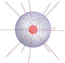
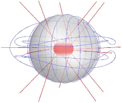
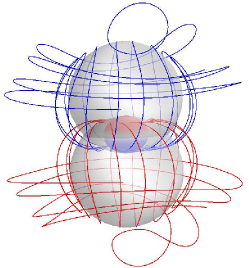
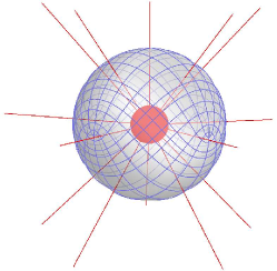
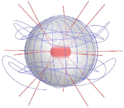
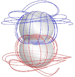
Figure 26: (color online). Tendex and vortex lines of Schwarzschild and Kerr black holes (of spin $a/M=0.945$) perturbed by a $(2,2)$ mode of either electric or magnetic parity, without removing the background tidal or frame-drag fields. The tendex lines and vortex lines are colored by the signs of their respective tendicities and vorticities (blue [dark gray] for positive and red [light gray] for negative). The horizons are colored and shaded by their vorticities or tendicities, and the transparent spheres have no physical significance, but they help to add perspective to the figures. The top panels are electric-parity perturbations and the bottom panels are magnetic-parity ones. Left column: Tendex lines of Schwarzschild black holes. Middle column: Tendex lines of Kerr black holes. Right column: Vortex lines of Kerr black holes.

In this appendix, we show the tendex and vortex lines of Schwarzschild and Kerr black holes when we plot a small $(2,2)$ perturbation of either electric or magnetic parity on top of the background tidal or frame-drag fields in Fig. 26. Specifically, we plot the vortex and tendex lines of

$$\bm{\mathcal{E}}=\bm{\mathcal{E}}^{(0)}+\epsilon\bm{\mathcal{E}}^{(1)}\,,\quad\bm{\mathcal{B}}=\bm{\mathcal{B}}^{(0)}+\epsilon\bm{\mathcal{B}}^{(1)}\,,$$ (126)

where $\bm{\mathcal{E}}^{(0)}$ and $\bm{\mathcal{B}}^{(0)}$ are the stationary, unperturbed background fields (visualized in Paper II), $\bm{\mathcal{E}}^{(1)}$ and $\bm{\mathcal{B}}^{(1)}$ are the perturbations (visualized by themselves in Fig. 14), and $\epsilon$ is a constant that sets the scale of the perturbation. To describe the strength of the perturbation, we will compare the perturbative horizon tendicity or vorticity to the background tendicity (for Schwarzschild holes) and the tendicity or vorticity (for Kerr black holes). For the Schwarzschild black holes in Fig. 26, we chose $\mathcal{E}_{NN}^{(1)}/\mathcal{E}_{NN}^{(0)}\approx 2\times 10^{-4}$ for the electric-parity perturbations and $\mathcal{B}_{NN}^{(1)}/\mathcal{E}_{NN}^{(0)}\approx 2\times 10^{-4}$ for the magnetic-parity perturbations. For electric-parity perturbations of Kerr holes, we chose $\mathcal{E}_{NN}^{(1)}/\mathcal{E}_{NN}^{(0)}\approx 3.5\times 10^{-3}$ and $\mathcal{B}_{NN}^{(1)}/\mathcal{B}_{NN}^{(0)}\approx 3\times 10^{-3}$, and for the magnetic-parity perturbations the ratios we selected were $\mathcal{E}_{NN}^{(1)}/\mathcal{E}_{NN}^{(0)}\approx 2.5\times 10^{-3}$ and $\mathcal{B}_{NN}^{(1)}/\mathcal{B}_{NN}^{(0)}\approx 5\times 10^{-3}$. We anticipate that these images may be useful for comparing with the results of numerical-relativity simulations, in which there is more ambiguity about how to separate a spacetime into a stationary background and dynamical perturbations, and for which it may be more useful to visualize the full frame-drag and tidal fields.

In the top panels of Fig. 26 are electric-parity perturbations, and the bottom panels are magnetic-parity perturbations. The left column of images are tendex lines of Schwarzschild black holes, the center column are tendex lines of Kerr black holes of spin $a/M=0.945$, and the right column are the corresponding vortex lines of the perturbed Kerr black holes. The lines are colored by the sign of their tendicity or vorticity (blue [dark gray] for positive and red [light gray] for negative) and the horizons are colored by their tendicity or vorticity. The transparent spheres are placed in the figures to help guide the eye, and do not indicate any feature of the vortexes or tendexes.

In these figures, we must choose an amplitude for the perturbation (described in the first paragraph above). For the all the black holes, we make the perturbation sufficiently small that one cannot see the effect of the perturbation in either the horizon tendicity, or the red (light gray) radial tendex lines. For the Kerr holes, we also require that the amplitude of the perturbation is less than the difference of the tendicities of the two non-radial tendex lines at the equatorial plane and around the radius at which the angular lines reach closest to the horizon. With this choice, the angular tendex lines will retain some features of the unperturbed lines before they become more distorted by the perturbation in the regions near the poles.

First, we will describe the tendex lines of the Schwarzschild black holes. An unperturbed Schwarzschild black hole is spherically symmetric, the tendicity on a sphere of constant radius is constant, and, therefore, any direction tangent to the sphere is a valid tendex line. For a weakly perturbed Schwarzschild black hole, although the perturbation may be small, the perturbation restricted to a sphere of constant $r$ completely determines the variation in the tendicity, and, furthermore, it will determine the directions of the tendex lines. This is analogous to degenerate perturbation theory in quantum mechanics, in which the eigenstates of the perturbing Hamiltonian restricted to the subspace spanned by the degenerate eigenstates are treated as the unperturbed states within the degenerate subspace. In directions that are not degenerate, however, its effects are negligible.

We can now use these facts about degeneracy to understand the tendex lines in the angular direction. The tidal field in the strictly angular directions, Eq. (90c) will determine the structure of the tendex lines on the sphere. The angular dependence is determined by the transverse-traceless, electric-parity tensor harmonic (for the top-left panel), because the trace term in Eq. (90c) is proportional to the identity and will not lift the degeneracy of the tendex lines. We would expect, therefore, that the tendex lines in the angular direction would resemble those of transverse-traceless, $l=2$, $m=2$, gravitational waves generated by a time-dependent mass quadrupole. These were shown in Zimmerman et al. (2011); Nichols et al. (2011), and the pattern of the lines is nearly identical. The tendicity along the lines is quite different from those of a gravitational wave, because for the perturbed Schwarzschild black hole, the tendicity is primarily determined by the constant unperturbed value on the sphere. Nevertheless, the tendex lines on the sphere show a striking similarity to those of gravitational waves at infinity.

For the magnetic-parity perturbation (the bottom-left panel), the tendex lines are determined by an $l=2$, $m=2$, magnetic-parity tensor harmonic; consequently, we would expect that the lines would resemble those of transverse-traceless gravitational waves at infinity, produced by a time-dependent, current-quadrupole source. Those lines were shown in Zimmerman et al. (2011), and they appear identical. Once more, though, the value of the tendicity along the lines is set by the background Schwarzschild black hole for the lines in bottom-left panel of Fig. 26 (unlike the tendicity of the lines studied in Zimmerman et al. (2011)).

The degeneracy between the angular tendex and vortex lines can also be used to explain the tendex and vortex lines in the middle and right columns of Fig. 26, respectively. For both the tendex and vortex lines, when the lines are near the equatorial plane ($\theta=\pi/2$) they resemble the unperturbed lines, but as they head toward the poles, they begin to become perturbed. This happens because the perturbation is small compared to the difference in the eigenvalues near the equatorial plane, and the perturbations have little effect on the tendex or vortex lines. Near the poles, however, the background vorticities and tendicities in the angular directions become degenerate (see the discussion at the end of Apps. A and B of Paper II), and the perturbation restricted to the degenerate subspace controls the lines’ directions. In the vicinity of the poles, the degenerate subspace is a plane parallel to the equatorial plane, and the perturbative tendex lines must form a regular grid around these points. When we combine this observation with the parity of the perturbation, we see that the lines at the opposite poles must be either parallel or orthogonal. Thus, these few simple constraints combine to explain the relatively simple pattern of the vortex and tendex lines of the perturbation plus the background frame-drag and tidal fields.

References

- Owen et al. (2011) R. Owen, J. Brink, Y. Chen, J. D. Kaplan, G. Lovelace, K. D. Matthews, D. A. Nichols, M. A. Scheel, F. Zhang, A. Zimmerman, et al., Phys. Rev. Lett. 106, 151101 (2011).
- Nichols et al. (2011) D. A. Nichols, R. Owen, F. Zhang, A. Zimmerman, J. Brink, Y. Chen, J. Kaplan, G. Lovelace, K. D. Matthews, M. A. Scheel, et al. (2011), eprint 1108.5486.
- Centrella et al. (2010) J. Centrella, J. G. Baker, B. J. Kelly, and J. R. van Meter, Rev. Mod. Phys. 82, 3069 (2010).
- Zhang et al. (2012) F. Zhang, A. Zimmerman, D. A. Nichols, Y. Chen, G. Lovelace, K. D. Matthews, R. Owen, and K. S. Thorne, Phys. Rev. D 86, 084049 (2012).