Constraining Source Redshift Distributions with Gravitational Lensing

Abstract

We introduce a new method for constraining the redshift distribution of a set of galaxies, using weak gravitational lensing shear. Instead of using observed shears and redshifts to constrain cosmological parameters, we ask how well the shears around clusters can constrain the redshifts, assuming fixed cosmological parameters. This provides a check on photometric redshifts, independent of source spectral energy distribution properties and therefore free of confounding factors such as misidentification of spectral breaks. We find that $\sim 40$ massive ($\sigma_{v}=1200$ km s^-1) cluster lenses are sufficient to determine the fraction of sources in each of six coarse redshift bins to $\sim$11%, given weak (20%) priors on the masses of the highest-redshift lenses, tight (5%) priors on the masses of the lowest-redshift lenses, and only modest (20-50%) priors on calibration and evolution effects. Additional massive lenses drive down uncertainties as $N_{\rm lens}^{-{1\over 2}}$, but the improvement slows as one is forced to use lenses further down the mass function. Future large surveys contain enough clusters to reach 1% precision in the bin fractions if the tight lens mass priors can be maintained for large samples of lenses. In practice this will be difficult to achieve, but the method may be valuable as a complement to other more precise methods because it is based on different physics and therefore has different systematic errors.

1. Introduction

Photometric redshifts are of key importance to current and future galaxy surveys. In a typical application, galaxies might be binned according to photometric redshift and then some analysis conducted on these binned source sets. Avoiding systematic error in this case requires knowledge of the true redshift distribution of each photometric redshift bin. Ideally, photometric redshift methods themselves produce reliable confidence intervals for this purpose, but external verification is important for controlling and quantifying systematic errors. For deep surveys, direct verification with a spectroscopic sample representative of the photometric sample is very difficult, and this has led to the development of other methods such as cross-correlating each photometric redshift bin with other photometric redshift bins (Schneider et al. 2006, Erben et al. 2009) or with spectroscopic redshift bins (Newman 2008, Matthews & Newman 2010). Here we present a new and independent method for reconstructing source redshift distributions, using the shear from weak gravitational lensing.

The shear induced by a given lens grows with source redshift in a well-understoood way which depends on cosmographic parameters. Other authors (Jain & Taylor 2003, Bernstein & Jain 2004) have suggested using this dependence to constrain the cosmographic parameters from the observed shear-vs-redshift relation around identified lenses. (Note that this is distinct from cosmic shear, for which the redshift dependence also involves the growth of structure.) In this paper we reverse the question and ask how well the redshift distribution of a set of galaxies can be constrained by shear measurements around lenses at a range of redshifts, if the background cosmology is already well determined (see Appendix A for a demonstration that cosmological uncertainties are negligible here). This may prove useful for applications which take the background cosmology as given, and it also provides an internal consistency check for surveys.

Although the shear around any given lens is rather weak and might be expected to provide very little constraint, a very large survey such as LSST (Iveziĉ et al. 2008) will contain billions of sources lensed by tens of thousands of galaxy clusters. Assuming the photometry is uniform over the sky, the entire dataset can be used to constrain the source redshift distribution. In this paper we use Fisher matrix formalism to estimate an upper bound on the effectiveness of this method, and we discuss challenges to implementing the method on real data. Because this method requires a very large survey, we refer to LSST throughout. We refer the reader to the LSST Science Book (LSST Science Collaborations et al. 2009) for more details on LSST survey parameters.

2. Basic idea and toy model

The tangential shear $\gamma$ at a projected distance $r$ around an axisymmetric lens is:

$$\gamma(r)={4\pi G\over c^{2}}{D_{ls}D_{l}\over D_{s}}[\bar{\Sigma}(<r)-\Sigma(r)]$$ (1)

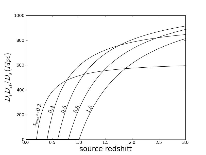
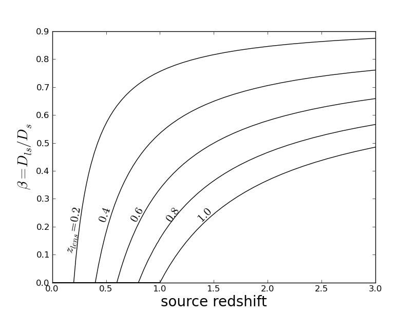
where $D_{ls}$, $D_{l}$, and $D_{s}$ are respectively the angular diameter distances from lens to source, observer to lens, and observer to source, $\Sigma(r)$ is the projected surface mass density at $r$, and $\bar{\Sigma}(<r)$ is the mean projected surface mass density within $r$ (Miralda-Escudè 1991). Figure 1 (top panel) shows the behavior of the distance factor ${D_{ls}D_{s}\over D_{s}}$ as a function of source redshift, for various fixed lens redshifts. This depends on the assumed cosmological model; we assume a WMAP7 $\Lambda$CDM cosmology of $H_{0}=70.4$ km s^-1 Mpc ^-1, $\Omega_{m}=0.272$, and $\Omega_{\Lambda}=0.728$ throughout. It is clear that very low-redshift ($z<0.2$) source galaxies will have no measurable shear around any of the lenses in the figure, moderate-redshift ($\sim 0.5$) sources will have measurable shear only around the lower-redshift lenses, and high-redshift ($z>1$) sources will have measurable shear around all lenses. This is the conceptual basis for constraining the redshift distribution of a source set: one should be able to solve for the source redshift distribution which, when passed through the appropriate response curves, best matches the observed shears. The method requires lenses at a range of redshifts and, to obtain good constraints, some prior knowledge of the lens masses. To simplify the exposition we treat the lens propertise as known in this section, and explore requirements on prior knowledge of lens properties in the next section.

Figure 1.— Top: The distance factor ${D_{ls}D_{l}\over D_{s}}$ as a function of source redshift, for various fixed lens redshifts. The lens redshift for each curve can be read off at the point where the curve departs from zero. Bottom: as for the left panel, but plotting $\beta={D_{ls}\over D_{s}}$.

Individual galaxies as well as clusters of galaxies can serve as lenses. Typically, the shear one arcminute off axis might be of order 0.5 for clusters and 0.01 for galaxies. Galaxies have near-isothermal mass profiles (Gavazzi et al. 2007), in which $\Sigma(r)$ and $\bar{\Sigma}(<r)$ scale as $r^{-1}$; specifically, $\bar{\Sigma}(<r)-\Sigma(r)={\sigma_{v}^{2}\over 2Gr}$ where $\sigma_{v}$ is the velocity dispersion. Because this scales as $r^{-1}$, it scales as $(\theta D_{l})^{-1}$ in terms of projected angular distance $\theta$, and $\gamma(\theta)$ can be written

$$\gamma(\theta)={2\pi\over c^{2}}{D_{ls}\over D_{s}}{\sigma_{v}^{2}\over\theta}$$

Isothermal lenses thus have the convenient property that $\gamma(\theta)$ can be separated into a part which depends only on the cosmology and a part which depends only on the mass or velocity dispersion of the lens. Mass profiles which are not scale-free cannot be written this way because the conversion from physical to angular scales invokes the cosmological model through $D_{l}$. This convenience is not required for our argument, but will substantially simplify the exposition here. Although cluster mass profiles depart from isothermality more than galaxy profiles do, for this section we will assume isothermality to simplify our argument.

We can now write a very simple model for the shear of the $i$th source galaxy due to the $j$th lens. We henceforth refer to $\sigma_{v}$ as $s$ to eliminate confusion with the symbol $\sigma$ which we will use later to indicate uncertainties on measurements. We also define $\beta={D_{ls}\over D_{s}}$ (taking $\beta$ to be zero where $z_{s}\leq z_{l}$); the $\beta$ curves for various lenses are shown in the bottom panel of Figure 1. We can then write

$$\gamma_{ij}={2\pi\over c^{2}}\beta_{ij}{s_{j}^{2}\over\theta_{ij}}$$ (2)

where $\theta_{ij}$ is the angular separation between lens $j$ and source $i$, $\beta_{ij}$ is the distance ratio between the two, and $s_{j}$ is the velocity dispersion of lens $j$.

The redshift distribution of the source set can be parameterized in many ways. Here we adopt the simplest approach, uniform bins in redshift. With $N_{\rm bin}$ bins, we parametrize the distribution with $f_{1},f_{2},...f_{N_{\rm bin}}$, where $f_{m}$ is the fraction of the galaxies in the set which are actually in redshift bin $m$. The highest-redshift bin should extend to arbitrarily high redshift so that none of the measured shear can come from an unmodeled part of the distribution. Consequently, we do not require that $\sum_{m}f_{m}=1$; any difference between unity and $\sum_{m}f_{m}$ can be interpreted as due to sources at such low redshift that they are never lensed. (A derived parameter $f_{0}\equiv 1-\sum_{m}f_{m}$ can be defined which encodes the fraction of sources at ultralow redshifts, but is not a parameter we solve for directly.) For sources from an unknown redshift distribution, the expected value of $\beta$ is simply $\sum_{m}f_{m}\beta_{mj}$, where $\beta_{mj}$ is now the mean distance ratio between lens $j$ and source redshift bin $m$. Thus the expected shear for a lens-source combination is

$$\langle\gamma_{ij}\rangle={2\pi\over c^{2}}{s_{j}^{2}\over\theta_{ij}}\sum_{m}f_{m}\beta_{mj}$$ (3)

In this section, we will assume that $s_{j}$ is perfectly known; we will consider uncertainty in lens masses in §3.

The observable is the total shear on each source galaxy due to all lenses which, in the weak lensing limit, is $\gamma_{i}=\sum_{j}\gamma_{ij}$. However, we must add shears componentwise because in the multiple-deflector context there is no longer a single “tangential” component. Thus shear is usually written as a complex quantity:

$$\langle\gamma_{ij}\rangle={2\pi\over c^{2}}{s_{j}^{2}\over\theta_{ij}}e^{i2\phi_{ij}}\sum_{m}f_{m}\beta_{mj}$$

where $\phi_{ij}$ is the position angle of source $i$ with respect to lens $j$, and the $i$ in the exponent represents $\sqrt{-1}$. The total expected shear on the source is then

$$\langle\gamma_{i}\rangle=\sum_{j}{2\pi\over c^{2}}{s_{j}^{2}\over\theta_{ij}}e^{i2\phi_{ij}}\sum_{m}f_{m}\beta_{mj}.$$

We could form a Fisher matrix with each two-component $\gamma_{i}$ contributing two observables; the derivatives of these observables with respect to the model parameters $f_{m}$ are very straightforward. However, this is computationally inefficient because most sources will be far from any modeled lens (assuming we use massive clusters rather than individual galaxies as the lenses) and thus will contribute negligible information to the Fisher matrix; and of the remaining sources, most are near only one lens so that their contribution can be captured by a single (tangential) component. Thus, at the expense of very little information, we can efficiently group sources according to their relevant lenses.

To do this, we group the observables in Equation 3 on one side and the model parameters on the other:

$$\langle\gamma_{ij}\theta_{ij}\rangle={2\pi\over c^{2}}{s_{j}^{2}}\sum_{m}f_{m}\beta_{mj}.$$ (4)

The $e^{i2\phi_{ij}}$ factor no longer appears because with only one lens involved the tangential component is unambiguous. We can collapse this down to a single observable for each lens by taking a mean of sources relevant to that lens:

$$\Gamma_{j}\equiv\langle\gamma_{ij}\theta_{ij}\rangle_{i\in j}={2\pi\over c^{2}}{s_{j}^{2}}\sum_{m}f_{m}\beta_{mj}$$ (5)

where ${i\in j}$ denotes averaging over all sources projected close enough to lens $j$ to add non-negligible information to the Fisher matrix. Accordingly,

$${\partial\Gamma_{j}\over\partial f_{m}}={2\pi s_{j}^{2}\over c^{2}}\beta_{mj}$$ (6)

To construct the Fisher matrix elements, we also need the variance of $\Gamma_{j}$. Because there is essentially no uncertainty on $\theta_{ij}$, the variance of $\gamma_{ij}\theta_{ij}$ is $\sigma_{i}^{2}\theta_{ij}^{2}$ where $\sigma_{i}$ is the uncertainty on the measured shear of galaxy $i$. Furthermore, $\sigma_{i}$ is uncorrelated with position or lens, so we can approximate it as a constant $\sigma_{\gamma}$ and pull it out of any sums. Weighting sources by inverse variance when computing $\Gamma_{j}$, we then find that

$$\sigma_{\Gamma_{j}}^{-2}=\sigma_{\gamma}^{-2}\sum_{i\in j}{1\over\theta_{ij}^{2}}$$ (7)

This sum primarily involves properties of the survey rather than the lens. We can rewrite it as the integral of the areal density of the source set, $n$, over the “footprint” of the lens, that is, the area over which the lens contributes non-negligible Fisher information: $n\int\theta^{-2}dA$. (Note that $n$ here is in units of galaxies per steradian, because $\theta$ is in units of radians. We will convert to the more typically quoted units of arcmin^-2 at the end of the calculation.) We shall see that the value of this integral is only weakly related to the properties of the lens. Integrating from some $\theta_{\rm min}$ to some $\theta_{\rm max}$ yields

$$n\int\theta^{-2}dA = 2\pi n\int_{\theta_{\rm min}}^{\theta_{\rm max}}\theta^{-1}d\theta$$ (8)

$$= 2\pi n\ln(\frac{\theta_{\rm max}}{\theta_{\rm min}})$$ (9)

Because the dependence is only logarithmic, we can make a rough estimate of $\frac{\theta_{\rm max}}{\theta_{\rm min}}$ for a typical lens and apply it to all lenses without much loss of precision. Sources less than $\sim 1$${}^{\prime}\,$ from the lens center are typically not used in weak lensing analyses because of the risk of contamination by cluster members and/or errors on their shear measurements due to background gradients from cluster members, so we adopt this value of $\theta_{\rm min}$. At large enough $\theta$, shear from unrelated structures will dominate the shear from the cluster. Although information about the cluster is still there, as a practical matter the effort to recover it may not be justified given the logarithmic dependence on $\theta_{\rm max}$. The shear around a massive cluster can clearly be observed out to at least $15$${}^{\prime}\,$ from the center (e.g, Kling et al. 2005), so $\theta_{\rm max}=15$${}^{\prime}\,$ should be a conservative value. Thus Equation 9 is approximately equal to $17n$, and only weakly dependent on the adopted values of $\theta_{\rm min}$ and $\theta_{\rm max}$. We expect the dependence on assumed shear profile to be weak as well, given that many ground-based weak-lensing cluster studies have difficulty discriminating between different forms of shear profiles (Wittman 2002). Inserting this result into Equation 7, we find that

$$\sigma_{\Gamma_{j}}^{2}=\frac{\sigma_{\gamma}^{2}}{17n}.$$

Assuming a Gaussian likelihood model, we now have an $N_{\rm bin}$ by $N_{\rm bin}$ Fisher matrix:

$$\mathcal{F}_{mn} = \sum_{j}^{N_{\rm lens}}{1\over\sigma_{\Gamma_{j}}^{2}}{\partial\Gamma_{j}\over\partial f_{m}}{\partial\Gamma_{j}\over\partial f_{n}}$$ (10)

$$= \left({2\pi\over c^{2}}\right)^{2}{17n\over\sigma_{\gamma}^{2}}\sum_{j}^{N_{\rm lens}}s_{j}^{4}\beta_{mj}\beta_{nj}$$ (11)

$$\approx 25(\frac{n}{\rm arcmin^{-2}})\sum_{j}^{N_{\rm lens}}(\frac{s_{j}}{\rm 1000\ km\ s^{-1}})^{4}\beta_{mj}\beta_{nj}$$ (12)

where we have adopted $\sigma_{\gamma}=0.2$, which represents the irreducible “shape noise” due to the random intrinsic orientations of sources. Smaller, fainter, sources will have larger shear uncertainties due to measurement uncertainties: $\sigma_{i}^{2}=\sigma_{\gamma}^{2}+\sigma_{{\rm meas},i}^{2}$. We account for this by defining $n$ as the effective source density, that is, the equivalent number of perfectly measured sources provided by the source set: ${n}=\sigma_{\gamma}^{2}\sum{1\over\sigma_{\gamma}^{2}+\sigma_{{\rm meas},i}^{2}}$ where the sum is taken over a unit area of sky. This is the basis on which surveys or source sets should be quoted; see the explanation of Equation 14.7 in the LSST Science Book (LSST Science Collaborations et al. 2009) for a more detailed justification.

As a rough estimate of the potential of this method, we compute a Fisher matrix forecast for an LSST-depth ($n=40$ arcmin^-2) survey covering nineteen lenses with $\sigma_{v}=1200$ km s^-1 at redshifts $z=\{0.05,0.1,0.15,...,0.95\}$, which roughly corresponds to using the most massive lens in the sky at each redshift. We model six redshift bins: five covering $0<z\leq 1$ with equal spacing, plus a sixth bin containing all galaxies at $z>1$. The forecast uncertainties on $f_{m}$ are then $\{0.06,0.07,0.11,0.17,0.20,0.10\}$. The same Fisher information can be obtained using a larger number of less-massive lenses, but going beyond a small number of well-studied lenses introduces a new problem: lens parameters such as $\sigma_{v}$ will not be known precisely for all these lenses, and we must examine the effect of marginalizing over uncertainties in the lens properties.

3. Marginalizing over lens mass

The two lens parameters in this model are redshift and mass (or equivalently, velocity dispersion). Spectroscopic redshifts are available in the literature for thousands of clusters, particularly for the most massive ones which contribute the most Fisher information. But with large imaging surveys now finding more clusters than can be followed up with spectroscopic redshift confirmation, photometric redshifts for the lenses must be considered. Photometric redshifts are much more precise for clusters than for individual galaxies, even beyond the statistical effect of averaging many member galaxies. Because cluster members are preferentially early-type galaxies with well-established spectral energy distributions, their redshifts can be established with very high confidence. Furthermore, the accuracy of cluster photometric redshifts can be easily verified by spectroscopy of a representative subsample of clusters, whereas representativeness is very difficult to achieve in spectroscopic subsamples of individual galaxies. The LSST Science Book (LSST Science Collaborations et al 2009) forecasts photometric redshift uncertainties for modest (10${}^{14}M_{\odot}$) clusters as a function of redshift; their Figure 13.12 shows that the uncertainties are 0.01 or less for all $z\leq 1.1$ after a single visit (and for all $z\leq 1.9$ after ten years of the survey). This fixes the $\beta$ factors to within 0.01, which is far more precise than the masses will be known a priori. We can therefore safely ignore uncertainties in lens redshifts. In the remainder of this section, we focus on marginalizing over lens mass uncertainties.

We now regard the $s_{j}^{2}$ as nuisance parameters. We choose $s_{j}^{2}$ rather than $s_{j}$ simply for convenience: $s_{j}^{2}$ is conceptually convenient because it is linearly proportional to the shear, and this proportionality makes it fall out of the relevant Fisher matrix elements. From Equation 5 we have

$${\partial\Gamma_{j}\over\partial(s_{k}^{2})}=\begin{cases}{2\pi\over c^{2}}\sum_{m}f_{m}\beta_{mj}&\text{if $j=k$,}\\ 0&\text{otherwise.}\end{cases}$$ (13)

We now have a Fisher matrix which is $N_{\rm bin}+N_{\rm lens}$ elements square. The lower-right $N_{\rm lens}\times N_{\rm lens}$ block is diagonal, because ${\partial\Gamma_{j}\over\partial(s_{k}^{2})}=0$ where $j\neq k$. These diagonal elements look like the square of the first case in Equation 13. The upper-left $N_{\rm bin}\times N_{\rm bin}$ block contains only elements of the form in Equation 11, and the other blocks (the $N_{\rm lens}\times N_{\rm bin}$ block in the upper right and its transpose in the lower left) contain mixed terms. Note, however, that many of the elements in these latter blocks will be zero, corresponding to lens/bin combinations for which the bin redshift is lower than the lens redshift, and thus for which $\beta_{mj}=0$. In the upper left block, no elements will vanish unless all lenses are at a higher redshift than the lowest-redshift bin. Note that the $f_{m}$ now appear in the Fisher matrix, so we must adopt fiducial values. Fisher matrix estimates should not be trusted far from the fiducial values; see Albrecht et al. (2006) for a clear exposition of Fisher matrix limitations. We therefore adopt a uniform fiducial distribution for now, and examine the dependence on the fiducial distribution at the end of this section.

Next, we need a prior on the lens masses. With no prior, the lowest-redshift lens would have no constraining power at all, as any shear (or lack thereof) in the lowest-redshift bin could be explained as a result of arbitrarily large (or small) lens mass. Successively higher-redshift lenses would have some constraining power, but not much. We therefore explore the importance of this prior by running Fisher matrix forecasts with the lens set of the previous section, but with priors of 1%, 2%, 5%, 10%, and 20% on the lens masses assuming the fiducial $s_{j}=1200$ km s^-1. We implement this by adding to the Fisher matrix the inverse variance representing a Gaussian prior before inverting the Fisher matrix to obtain the covariance matrix. To implement the 1% prior, for example, we add $(0.01(1200^{2}))^{-2}$ to $\mathcal{F}_{7,7},\mathcal{F}_{8,8},...\mathcal{F}_{25,25}$, which are the nineteen elements representing the lens $s_{j}^{2}$. Figure 2 shows the results. For the low-redshift bins, obtaining constraints close to those of the previous section requires a 1-2% prior, but for higher-redshift bins the required priors are more modest, 10-20%. Priors tighter than 1% (not shown) do not yield any visible improvement in this figure.

Figure 2.— Constraints on the bin fractions for various lens-mass priors in the simplified physical scenario of §2 with just one massive lens at each redshift. The redshift-varying prior allows for weaker lens-mass priors at higher lens redshifts where priors are both less necessary and more difficult to establish observationally; this particular form is $5\%(1+z_{\rm lens})^{2}$ which brings the prior to 20% at $z_{\rm lens}=1$. More lenses of the same mass will tighten the constraints as $N_{\rm lens}^{-{1\over 2}}$.

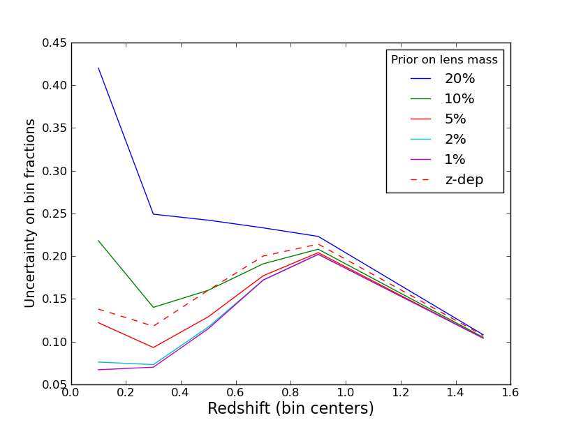
The most efficient observational approach may thus be to obtain tight priors on low-redshift lenses using velocity dispersions, X-ray analyses, external lensing analyses, etc, while obtaining only very rough priors on the higher-redshift lenses. We model this scenario by testing a mass prior which is 5% at $z_{\rm lens}=0$ but loosens as $(1+z_{\rm lens})^{2}$ (i.e., a 20% prior at $z_{\rm lens}=1$); this is is shown as the dashed curve in Figure 2. This yields source redshift constraints as good as those obtained with a 5-10% prior, but without much difficult high-redshift work. Indeed, optical richness alone can provide a 20-30% prior on the mass (Rykoff et al. 2011), thus obviating the need for followup at the high-redshift, assuming there is no redshift above which the optical richness estimator breaks down.

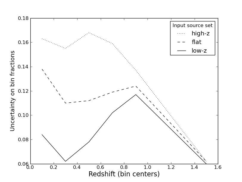
To a reasonable approximation, each additional lens tightens the constraints mostly on the 1-2 source redshift bins nearest the lens. Therefore, we can tweak the lens sample to obtain roughly equal constraints on all source redshift bins. For example, we see from Figure 2 that the maximum uncertainty for the efficient redshift-varying mass prior is for source redshifts 0.7-0.9, at a level of roughly twice the minimum uncertainty. Tripling the number of lenses at redshifts 0.5-0.95, for a total of 39 massive lenses, yields roughly equal constraints on most source redshift bins, averaging 0.11 (middle curve in Figure 3). Reaching yet lower levels of uncertainty requires more lenses overall. For example, reaching 0.01 uncertainty across the board will require $11^{2}$ times more lenses than the previous scenario, or about 5000 total. However, when so many lenses are considered, we cannot use only very massive lenses. Therefore, the required number of lenses will scale much more steeply than the inverse square of the desired constraint. The Fisher information corresponding to 5000 lenses with $\sigma_{v}=1200$ km s^-1 could be accumulated with tens of thousands of less-massive lenses, which is well within expectations for current and future large imaging surveys. Computationally, using so many lenses should be feasible because most of the tens of thousands of nuisance parameters can be marginalized over separately, reflecting the nonoverlapping nature of most lenses. However, the 1% goal will be difficult to achieve at low redshift due to the difficulty of obtaining the 5-8% lens-mass priors necessary to do so well there.

These factors provide insight into why we do not propose using individual galaxies as lenses. For every $10^{15}$ $M_{\odot}$ cluster, a survey would need one million $10^{12}$ $M_{\odot}$ galaxies to provide the same Fisher information, all other factors being equal. Although surveys such as LSST will have billions of galaxies, all other factors are not equal. The photometric redshift uncertainty on each individual galaxy is much larger than for clusters, and individual-galaxy lens photometric redshifts bring in exactly the problems this method is designed to avoid. These problems could be avoided by using only early-type galaxies with well-behaved photometric redshifts and mass priors from the fundamental plane, but then far too few lenses would be available. Furthermore, galaxy-scale lenses do not dominate their local shear in a way which allows parallelized modeling of designated patches of sky, and thus would introduce additional computational challenges.

A foreseeable application for this method is to input source sets corresponding to each of several photometric redshift bins, to determine the outlier fraction and distribution in each. Therefore, we examine the dependence on the redshift distribution of the source set, which we have assumed to be flat until now. Figure 3 shows the results using the redshift-varying mass prior and the 39 massive lenses with three different source sets: flat (as described above, middle curve), all in the $z<0.2$ bin (lower curve), and all in the $0.8<z\leq 1.0$ bin (upper curve). Characterization of outliers will be more precise for the low-$z_{\rm phot}$ source set than for the high-$z_{\rm phot}$ source set, although this is partly due to the choice of lens-mass prior which is tighter at lower redshift.

Figure 3.— Constraints on the bin fractions for low-redshift (lower curve), flat (middle curve), and high-redshift (upper curve) source sets. Each source set is used with the redshift-varying lens-mass prior and 39 lenses described in the text.

4. Profile and calibration uncertainties

To this point we have assumed that prior knowledge of a cluster’s velocity dispersion translates perfectly into prior knowledge of its integrated shear statistic, given a source redshift distribution. However, the relationship between these two observables is sure to be more complicated. Clusters with the same velocity dispersion may have different profiles, resulting in different integrated shear estimates. If this is a purely stochastic effect, then the scatter in the observable-observable relation weakens the prior. But in principle, the loss of information due to this scatter can be compensated by analyzing more clusters. Conceptually more worrisome would be a redshift-dependent trend or an overall calibration error in this relationship, which would cause systematic errors.

We therefore insert nuisance parameters describing the uncertainties in calibration and redshift evolution, and explore how the results degrade as priors on these parameters are relaxed. We allow Equation 5 to be multiplied by a factor $a+bz_{j}$, where $a$ is a nuisance parameter for the calibration, $b$ is a nuisance parameter for the redshift evolution, and $z_{j}$ is the redshift of the $j$th lens, and repeat the analysis of the previous section with the flat source distribution and the redshift-dependent lens mass prior. Figure 4 shows the reconstruction precision for a range of calibration and evolution priors, with a fiducial model of $a=1$ and $b=0$. Priors of 20% on each are sufficient to preserve performance nearly identical to that of the previous section in which calibration and evolution were not factors; the bottom curve in each panel is very similar to the middle curve in Figure 3.

Figure 4.— Constraints resulting from a range of calibration (top panel) and evolution (bottom panel) priors. For the top panel the evolution prior has been set to 20% in all cases, and for the bottom panel the calibration prior has been set to 20% in all cases. Priors tighter than 20% on either do not substantially improve the results: the bottom curve in each panel is very similar to the middle curve in Figure 3, where the priors were delta functions.

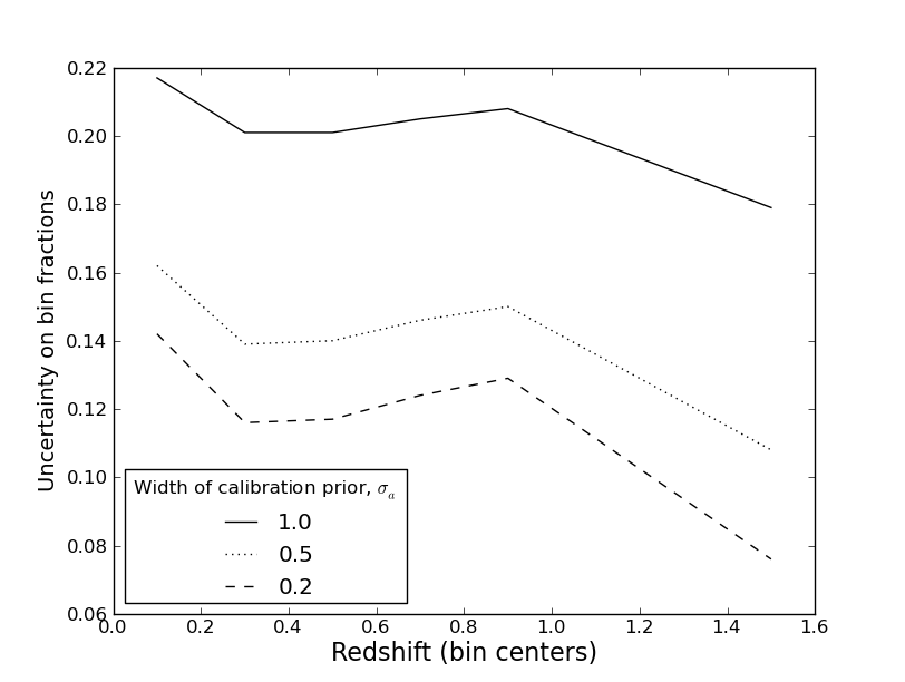
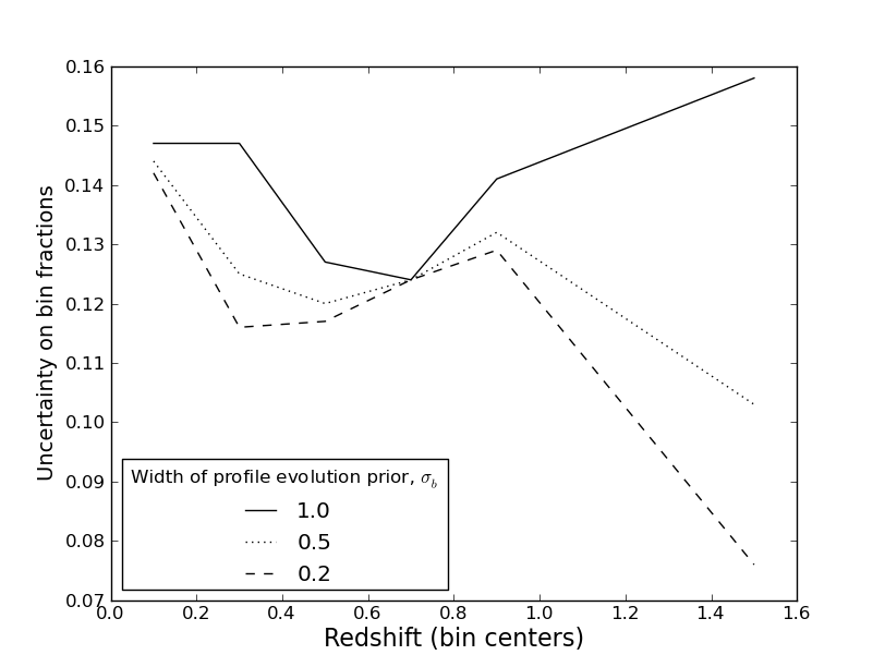
We stress that the choice of an isothermal profile as a calculation aid here is not fundamental to the method. In practice, surveys would measure the average cluster profile and construct an optimal integrated shear estimator before commencing the redshift analysis. The results of this section indicate that profile calibration and evolution uncertainties at the 20-50% level do not substantially degrade the performance of this method.

5. Discussion

We have outlined a new method which uses gravitational lensing by clusters and knowledge of the cosmology to constrain source redshift distributions. Although this is an unorthodox use of the lensing-redshift information, it has some strengths and some relevant applications. The method’s strengths are:

• it is independent of other methods. It relies on no assumptions about galaxy spectral properties or biasing.

• it is applicable to any set of galaxies. One can determine the redshift distribution of a set of galaxies chosen in any number of ways, such as photometric redshift cut, pure color selection, or even X-ray or radio selection. Multiwavelength observations are not necessary as they are for photometric redshifts.

• in the context of a large imaging survey, it requires little additional data. Where lens spectroscopic redshifts are not available, photometric lens redshifts will do, and optical richness provides a sufficient lens-mass prior for the high-redshift lenses. However, pinning down the low-redshift end of the source distribution will require strong mass priors on low-redshift lenses.

Our Fisher matrix forecast involves some approximations and caveats:

• Lens morphology: we have assumed axisymmetric isothermal lenses. Although we have argued that other profiles would not yield substantially different forecasts, a precise experiment would include some sort of marginalization over profiles. This marginalization might include allowances for non-axisymmetry.

• Foreground/background structure: we have assumed that shear from foreground/background structure is negligible in the “footprint” of each lens, and totally dominant outside. In reality, unmodeled shear will be present in the footprint as well, and contribute to slightly looser constraints. However, unmodeled shear is not an irreducible source of noise. One can choose to model previously unmodeled structure and thus add information to the Fisher matrix. This entails a cost-benefit analysis rather than a hard limit.

• Magnification: the observed source population behind lenses will be slightly different than in other locations, due to lensing magnification. If unmodeled, this may result in a nontrivial systematic error. However, because the lenses are being modeled, the model magnification at any given point provides an easily available basis for correction. Deep fields which establish the source counts fainter than the main survey flux limit will be very useful for this purpose. As with the foreground/background structure, it may be possible to add information to the Fisher matrix with improved modeling of the magnification.

• Cluster contamination: the areas around clusters differ from the general area of a survey in another respect, the presence of cluster members. Care must be taken so that the source set whose shear is being measured is not contaminated by these members.

• Cosmology dependence of $\beta$: Appendix A shows that marginalizing over uncertainty in cosmographic parameters will not degrade the results presented here. But using the cosmology as input here implies that the redshift estimates from this method should not feed in to some other method which estimates the cosmology unless the covariances are properly treated.

• Wide source redshift bins: given a lens redshift, $\beta$ varies over the width of a source redshift bin. Accurately modeling this effect will require some assumptions about the source redshift distribution inside the bins. It may be possible to find a parameterization which reduces this difficulty.

The source redshift distributions obtained with this method will be most useful in applications where the background cosmology would have been assumed anyway, such as galaxy evolution, and especially in applications which are very sensitive to photometric redshift outliers. For example, measurements of the bright end of the galaxy luminosity function at high photometric redshift are extremely sensitive to catastrophic outliers, as a small fraction of low-redshift galaxies mistakenly put at high redshift results in many more “high-luminosity” galaxies at that redshift. Surveys can use this method to independently derive the full redshift distribution of the galaxies in each photometric redshift bin, thus characterizing the number and distribution of outliers. Indeed, the use of multiwavelength photometry to infer both source redshift and source spectral/photometric properties can be problematic, and this method offers a possible workaround.

Other methods such as cross-correlation with a spectroscopic sample (Newman 2008, Matthews & Newman 2010) should be able to achieve 1% accuracy without assuming a cosmology or requiring expensive lens mass priors. This method may therefore not be competitive statistically, but as it is based on different physics it may offer value in having different systematic errors. Redshift distributions derived using this method can and should be used in consistency checks. Given the best-fit cosmology from weak lensing tomography, this method should produce source redshift distributions which are consistent with those used in the weak lensing tomography. A prime application for this method may therefore be as an internal consistency check for surveys.

Appendix A Dependence on Cosmological Parameters

This appendix justifies the assumption in the main body of the paper that uncertainties in the distance ratios contribute negligible uncertainty to the parameters of interest, the fraction of sources in each redshift bin. Uncertainty in the distance ratios comes from uncertainty in cosmographic parameters, including Hubble’s constant $H_{0}$ and the energy densities in matter ($\Omega_{m}$), curvature ($\Omega_{k}$), and in the cosmological constant ($\Omega_{\Lambda}$). Of course, more general dark energy models can introduce further parameters, but the cosmological constant has a greater effect on distances than a dark energy model with equation of state parameter $w>-1$. Therefore, if the assumption is justified for a cosmological constant model, it is justified for models with $w>-1$.

Distances depend linearly on Hubble’s constant $H_{0}$, but $\beta={D_{ls}\over D_{s}}$ is a ratio of distances. Therefore $\beta$ does not depend on $H_{0}$ and uncertainty in $H_{0}$ is irrelevant.

The remaining parameters are more difficult to treat analytically, so we make a numerical estimate. The derivatives of $\beta$ with respect to $\Omega_{m}$ and $\Omega_{\Lambda}$ (with $\Omega_{k}=1-\Omega_{m}-\Omega_{\Lambda}$) depend on the lens and source redshifts, but are typically of order 0.02. The worst case is for uncertainty in $\Omega_{m}$ when considering high-redshift sources and lenses, where ${\partial\beta\over\partial\Omega_{m}}\approx 0.15$. We take a conservative approach by setting ${\partial\beta\over\partial\Omega_{m}}=0.15$ for all sources and lenses, so that the partial derivative of Equation 5 with respect to $\Omega_{m}$ is 0.15 times ${2\pi\over c^{2}}s_{j}^{2}$. We include $\Omega_{m}$ as a parameter in the Fisher matrix using these partial derivatives.

We rerun the forecast with a Gaussian prior of $\sigma=0.016$ on $\Omega_{m}$, which corresponds to the current WMAP7+BAO+H0 uncertainty for the “OLCDM” model in which curvature is allowed to vary. If the results were plotted on Figure 2 or Figure 3, they would be nearly indistinguishable from the existing plots. The biggest difference would be the point in the lower right corner of Figure 3 increasing from 0.052 to 0.055. The effect of varying $\Omega_{\Lambda}$ is even smaller because $\beta$ is less sensitive to it.

References

- Albrecht at al. (2006) Albrecht, A., Bernstein, G., Cahn, R., et al. 2006, arXiv:astro-ph/0609591
- Bernstein & Jain (2004) Bernstein, G., & Jain, B. 2004, ApJ, 600, 17
- Erben et al. (2009) Erben, T., Hildebrandt, H., Lerchster, M., et al. 2009, A&A, 493, 1197
- Gavazzi et al. (2007) Gavazzi, R., Treu, T., Rhodes, J. D., et al. 2007, ApJ, 667, 176
- Ivezic et al. (2008) Ivezic, Z., Tyson, J. A., Acosta, E., et al. 2008, arXiv:0805.2366
- Jain & Taylor (2003) Jain, B., & Taylor, A. 2003, Physical Review Letters, 91, 141302
- Kling et al. (2005) Kling, T. P., Dell’Antonio, I., Wittman, D., & Tyson, J. A. 2005, ApJ, 625, 643
- LSST Science Collaborations et al. (2009) LSST Science Collaborations, Abell, P. A., Allison, J., et al. 2009, arXiv:0912.0201
- Matthews & Newman (2010) Matthews, D. J., & Newman, J. A. 2010, ApJ, 721, 456
- Miralda-Escude (1991) Miralda-Escude, J. 1991, ApJ, 370, 1
- Newman (2008) Newman, J. A. 2008, ApJ, 684, 88
- Rykoff et al. (2011) Rykoff, E. S., Koester, B. P., Rozo, E., et al. 2011, arXiv:1104.2089
- Schneider et al. (2006) Schneider, M., Knox, L., Zhan, H., & Connolly, A. 2006, ApJ, 651, 14
- Wittman (2002) Wittman, D. 2002, Gravitational Lensing: An Astrophysical Tool, 608, 55