Secular evolution of galaxies

Abstract

What else can be said about star formation rate indicators that has not been said already many times over? The ‘coming of age’ of large ground-based surveys and the unprecedented sensitivity, angular resolution and/or field-of-view of infrared and ultraviolet space missions have provided extensive, homogeneous data on both nearby and distant galaxies, which have been used to further our understanding of the strengths and pitfalls of many common star formation rate indicators. The synergy between these surveys has also enabled the calibration of indicators for use on scales that are comparable to those of star-forming regions, thus much smaller than an entire galaxy. These are being used to investigate star formation processes at the sub-galactic scale. I review progress in the field over the past decade or so.

[Daniela Calzetti]Daniela Calzetti
Department of Astronomy, University of Massachusetts,
710 North Pleasant Street, Amherst, MA 01003, USA,
calzetti@astro.umass.edu

Chapter Star formation rate indicators

1 Introductory remarks

My goal for this chapter, based on a series of lectures at the XXIII Canary Islands Winter School of Astrophysics, is to present current understanding and calibrations of star formation rate (SFR) indicators, both on global, galaxy-wide scales, and on local, sub-galactic scales. SFRs are, together with masses, the most important parameters that define galaxies and their evolution across cosmic times. Although SFR calibrations have existed, with various levels of accuracy, for many years and sometimes decades, the past eight to ten years have brought forth major progress, through cohesive, multi-wavelength surveys of nearby and distant galaxies. These surveys have exploited the sensitivity, angular resolution and/or large field of view of space telescopes (e.g., the Spitzer Space Telescope, the Galaxy Evolution Explorer [GALEX], the Hubble Space Telescope [HST], and the Herschel Space Telescope) and leveraged the multi-band coverage supplied by ground-based, all-sky surveys (e.g., the Sloan Digital Sky Survey), in order to push the definition of SFR indicators into new regimes, both in terms of wavelength coverage and spatial scales. I review here recent progress in this area, but also highlight where challenges, sometimes unexpected ones, have arisen. This chapter is structured to provide also a quick reference for the relevant literature on SFR calibrations. It loosely follows the structure of the lectures I presented at the Winter School.

2 Calibration of star formation rate indicators across the wavelength spectrum

Calibrations of SFR indicators have been presented in the literature for almost 30 years, derived across the full electromagnetic spectrum, from the X-ray, through the ultraviolet (UV), via the optical and infrared (IR), all the way to the radio, and using both continuum and line emission (see review by Kennicutt 1998, and, e.g., Donas & Deharveng 1984; Yun et al. 2001; Kewley et al. 2002, 2004; Ranalli et al. 2003; Bell 2003; Calzetti et al. 2005, 2007, 2010; Schmitt et al. 2006; Alonso-Herrero et al. 2006; Moustakas et al. 2006; Salim et al. 2007; Persic & Rephaeli 2007; Rosa-González et al. 2007; Kennicutt et al. 2007, 2009; Rieke et al. 2009; Lawton et al. 2010; Boquien et al. 2010; Verley et al. 2010; Li et al. 2010; Treyer et al. 2010; Murphy et al. 2011; Hao et al. 2011). The most recent review on the subject is by Kennicutt & Evans (2012).

Recent findings that most of the star formation at redshift $z\sim$1–3 was enshrouded in dust (Le Floch et al. 2005; Magnelli et al. 2009; Elbaz et al. 2011; Murphy et al. 2011b; Reddy et al. 2012) have renewed interest in IR SFR indicators, particularly in the monochromatic (single-bands) ones, which can be in principle as straightforward to use as those already available at UV and optical wavelengths. This interest has been aided by the advent of high-angular resolution, high-sensitivity IR space telescopes (Spitzer, Herschel), that have enabled the calibration of monochromatic SFR indicators in nearby galaxies. The IR investigations complement efforts at UV and optical wavelengths to chart the SFR evolution of galaxies from redshift $\sim$7–10 to the present (e.g., Giavalisco et al. 2004; Bouwens et al. 2009, 2010). The UV and optical may be the preferred SFR indicators at very high redshift, when galaxies contained little dust (e.g., Wilkins et al. 2011; Walter et al. 2012). The calibration of SFR indicators remains, however, a central issue for studies of distant galaxies (e.g., Reddy et al. 2010; Lee et al. 2010; Wuyts et al. 2012), since it can be affected by differences in star formation histories, metal abundances, content and distribution of stellar populations and dust between low and high redshift galaxies (Elbaz et al. 2011), and, possibly, by cosmic variations in the cluster mass function and stellar initial mass function (IMF, Wilkins et al. 2008; Pflamm-Altenburg et al. 2009).

Throughout this chapter, I refer to two categories of SFR calibrations: (1) ‘global’, i.e., defined for whole galaxies, thus they are luminosity-weighted averages across local variations in star formation history and physical conditions within each galaxy; and (2) ‘local’, i.e., defined for measuring SFRs in regions within galaxies, on sub-galactic/sub-kpc scale (e.g., Wu et al. 2005; Alonso-Herrero et al. 2006; Calzetti et al. 2005, 2007, 2010; Zhu et al. 2008; Rieke et al. 2009; Kennicutt et al. 2009; Lawton et al. 2010; Boquien et al. 2010, 2011; Verley et al. 2010; Li et al. 2010; Treyer et al. 2010; Liu et al. 2011; Hao et al. 2011; Murphy et al. 2011). While global SFR calibrations have received most of the attention in the past, both for objective limitations in the spatial resolution of the data and for their broader applicability to distant galaxy populations, local SFR calibrations have become increasingly prominent in the literature as important tools to investigate the physical processes of star formation.

The definition of a local SFR can, however, be problematic if referring to too small a region: for instance a single star cluster that formed almost instantaneously 15 Myr ago has a current SFR=0 (it is no longer forming stars), although stars were clearly formed in the recent past. To avoid such extreme situations, local SFRs are meant to refer to measurements performed on areas that include multiple star-forming regions, so that star formation can be considered constant over the relevant timescale for the SFR indicator used. For all practical purposes, such regions tend to be a few hundred pc across or larger.

In general, global calibrations are not necessarily applicable to local conditions and vice versa. The fundamental reason is that while the stellar and dust emission from entire galaxies can be treated, in first approximation, as if the galaxy were an isolated system, the same is not necessarily true for a sub-galactic region. Stellar populations mix within galaxies on timescales that are comparable to those of their UV light lifetime. The stellar IMF (i.e., the distribution of stellar masses at birth) may or may not be fully sampled locally. The star formation history may vary from region to region. Both young and old stars can heat the dust in a galaxy, and the dust spectral energy distribution (SED) and features provide little discrimination as to the source of the heating. Because of all these reasons, local SFR indicators are by far less settled than the global ones.

In what follows, I will discriminate between global and local SFR indicators, when appropriate. All calibrations are given for a Solar metallicity stellar population, when models are used.

2.1 General characteristics

Techniques for measuring the rate at which stars are being formed vary enormously, also depending on whether the target system is resolved into individual units (e.g., young stars) or not. In all cases, however, the basic goal is to identify emission that probes newly or recently formed stars, while avoiding as much as possible contributions from evolved stellar populations.

The timescale over which ‘recent’ is a valid word also varies between different applications and among different systems, but free-fall times $\tau_{\rm ff}$ probably provide a reasonable ballpark scale. Most researchers would agree that ‘recent’ refers to timescales $\approx$10–100 Myr when considering whole galaxies, and $\approx$1–10 Myr when considering regions or structures within galaxies (e.g., giant molecular clouds, etc.).

The most common approach for measuring SFRs in resolved regions, such as regions within the Milky Way, is to count individual objects or events (e.g., supernovae) that trace the recent star formation (Chomiuk & Povich 2011). In the molecular clouds within 0.5–1 kpc of the solar system, this is accomplished by counting young stellar objects (YSOs), i.e., protostars at different stages of evolution, which, because they are still embedded in their natal clouds, are optimally identified in the IR. The total number of YSOs is converted to a SFR via:

$${\rm SFR(YSO)}=N_{\rm YSO}\frac{\langle M\rangle}{\tau}$$ (1)

where the mean YSO mass, $\langle M\rangle$ depends weakly on the adopted stellar IMF (see Section 2.2), and the lifetime of a YSO is, with some uncertainty, $\tau\sim$2 Myr (Evans et al. 2009; Heidermann et al. 2010; Gutermuth et al. 2011). The SFR(YSO) is in units of $M_{\odot}$ yr^-1.

In unresolved systems, SFR indicators are merely measures of luminosity, either monochromatic or integrated over some wavelength range, with the goal of targeting continuum or line emission that is sensitive to the short-lived massive stars. The conversion from the luminosity of massive stars to a SFR is performed under the assumption that: (1) the star formation has been roughly constant over the timescale probed by the specific emission being used; (2) the stellar IMF is known (or is a controllable parameter) so that the number of massive stars can be extrapolated to the total number of high$+$low mass stars formed; and (3) the stellar IMF is fully sampled, meaning that at least one star is formed in the highest-mass bin, and all other mass bins are populated accordingly with one or more stars (see discussion in Section 2.2).

SFR indicators in the UV/optical/near-IR range ($\sim$0.1-5 $\mu$m) probe the direct stellar light emerging from galaxies, while SFR indicators in the mid/far-IR ($\sim$5–1000 $\mu$m) probe the stellar light reprocessed by dust. In addition to direct or indirect stellar emission, the ionising photon rate, as traced by the gas ionised by massive stars, can be used to define SFR indicators; photo-ionised gas usually dominates over shock-ionised gas in galaxies or large structures within galaxies (e.g., Calzetti et al. 2004; Hong et al. 2011). Tracers include hydrogen recombination lines, from the optical, through the near-IR, all the way to radio wavelengths, forbidden metal lines, and, in the millimetre range, the free-free (Bremsstrahlung) emission. The X-ray emission produced by high-mass X-ray binaries, massive stars, and supernovae can also, in principle, be used to trace SFRs. Finally, the synchrotron emission from galaxies can be calibrated as a SFR indicator (Condon 1992), since cosmic rays are produced and accelerated in supernova remnants, and core-collapse supernovae represent 70% or more of the total supernovae in star-forming galaxies (Bossier & Prantzos 2009).

The following five subsections describe in more detail a few of these SFR indicators for unresolved systems. The emission contribution to the galaxy luminosity from a potential active galactic nuclei (AGN) can be large, depending on the galaxy type and the wavelength of the SFR indicator. I assume that this potential contribution has been recognised and removed from the emission that is being used as a SFR indicator.

2.1.1 Indicators based on direct stellar light

The youngest stellar populations emit the bulk of their energy in the restframe UV ($<$0.3 $\mu$m); in the absence of dust attenuation, this is the wavelength range ‘par excellence’ to investigate star formation in galaxies over timescales of $\approx$100–300 Myr, since both O and B stars are brighter in the UV than at longer wavelengths. As a reference, the lifetime of an O6 star is $\sim$6 Myr, and that of a B8 star is $\sim$350 Myr. The luminosity ratio at 0.16 $\mu$m of an O6 to a B8 star is $\sim$90, but, if the stellar population follows a Kroupa (2001) IMF (see Section 2.2), for every O6 star formed, about 150 B8 stars are formed. Thus, at age zero, the UV emission from the collective contribution of B8 stars is comparable to that of O6 stars.

For a Kroupa stellar IMF, with constant star formation over 100 Myr, the non-ionising UV ($0.0912\mu{\rm m}<\lambda<0.3\mu{\rm m}$) stellar continuum can be converted to a SFR:

$${\rm SFR(UV)}=3.0\cdot 10^{-47}\lambda L(\lambda)$$ (2)

with SFR(UV) in $M_{\odot}$ yr^-1, $\lambda$ in Å, and L($\lambda$) in erg/s. The stellar SED used for this calibration is from Starburst99, with solar metallicity (Leitherer et al. 1999). The accuracy of the calibration constant is $\pm$15%, which takes into account small variations as a function of $\lambda$.

For constant star formation over timescales longer than 100 Myr, the calibration constant only decreases by a few percent. However, for shorter timescales, changes are more significant. For $\tau$=10 Myr and 2 Myr, the constant is about 42% and a factor 3.45, respectively, higher than in Equation 2 (Table 1). This shows that if star formation has been active in a region on a timescale shorter than about 100 Myr, the cumulative UV emission of massive stars is still increasing in luminosity, and the calibration of any SFR(UV) indicator has to take this fact into account.

Table 1: Model-based luminosity-to-SFR calibrations

Luminositya	$C^{b}$	Assumptionsc
L(UV)	3.0$\times 10^{-47}\lambda$	0.1–100 $M_{\odot}$, $\tau\geq$100 Myr
L(UV)	4.2$\times 10^{-47}\lambda$	0.1–30 $M_{\odot}$, $\tau\geq$100 Myr
L(UV)	4.3$\times 10^{-47}\lambda$	0.1–100 $M_{\odot}$, $\tau$=10 Myr
L(UV)	1.0$\times 10^{-46}\lambda$	0.1–100 $M_{\odot}$, $\tau$=2 Myr
L(TIR)	1.6$\times 10^{-44}$	0.1–100 $M_{\odot}$, $\tau$=10 Gyr
L(TIR)	2.8$\times 10^{-44}$	0.1–100 $M_{\odot}$, $\tau$=100 Myr
L(TIR)	4.1$\times 10^{-44}$	0.1–30 $M_{\odot}$, $\tau$=100 Myr
L(TIR)	3.7$\times 10^{-44}$	0.1–100 $M_{\odot}$, $\tau$=10 Myr
L(TIR)	8.3$\times 10^{-44}$	0.1–100 $M_{\odot}$, $\tau$=2 Myr
L(H$\alpha$)	5.5$\times 10^{-42}$	0.1–100 $M_{\odot}$, $\tau\geq$6 Myr, $T_{\rm e}$=104 k, $n_{\rm e}$=100 cm-3
L(H$\alpha$)	3.1$\times 10^{-41}$	0.1–30 $M_{\odot}$, $\tau\geq$10 Myr, $T_{\rm e}$=104 k, $n_{\rm e}$=100 cm-3
L(Br$\gamma$)	5.7$\times 10^{-40}$	0.1–100 $M_{\odot}$, $\tau\geq$6 Myr, $T_{\rm e}$=104 k, $n_{\rm e}$=100 cm-3

A more subtle, but not less important, effect is caused by the length of time over which a stellar SED remains relatively bright in the UV. This is due to the significant UV emission of mid-to-late B stars. For example, a constant star formation event of 10 Myr duration, which, at constant SFR=1 $M_{\odot}$ yr^-1, accumulates 10⁷ $M_{\odot}$ in stars, has the same UV luminosity and a similar UV SED over the range 0.13–0.25 $\mu$m of a 50 Myr old, 2.5$\times$10⁸ $M_{\odot}$ instantaneous burst of star formation. In the absence of dust attenuation and if only observed in the UV, the two populations would be attributed the same SFR(UV)=1 $M_{\odot}$ yr^-1. While this number is correct for the first population, it would be incorrect, and possibly misleading, for the second population (which has not been forming stars since 50 Myr). If dust attenuation is also present, the potential of misclassifying an ageing population for an active star-forming one increases.

As the vast majority of galaxies contain at least some dust, the use of SFR(UV) becomes complicated, since dust attenuation corrections are usually required, and are uncertain. For the most part dust corrections only work on ensembles of systems, rather than individual objects. In a show of Cosmic Conspiracy, the most active and luminous systems are also richer in dust, implying that they require more substantial corrections for the effects of dust attenuation (Wang & Heckman 1996; Calzetti 2001; Hopkins et al. 2001; Sullivan et al. 2001; Calzetti et al. 2007). As a reference number, a modest optical attenuation $A_{V}$=0.9 produces a factor ten reduction in the UV continuum at 0.13 $\mu$m, if the attenuation curve follows the recipe of Calzetti et al. (2000).

2.1.2 Indicators based on dust-processed stellar light

The IR luminosity of a system will depend not only on its dust content, but also on the heating rate provided by the stars. To first order, the shape of the thermal IR SED will depend on the starlight SED, in the sense that UV-luminous, young stars will heat the dust to higher mean temperatures than old stellar populations (e.g., Helou 1986).

Because of the properties of the Planck function, hotter dust in thermal equilibrium has higher emissivity in the IR than cooler dust. Furthermore, the cross-section of the dust grains for stellar light is higher in the UV than in the optical, as inferred from the typical trend of interstellar extinction curves. Thus, qualitatively, the dust heated by UV-luminous, young stellar populations will produce an IR SED that is more luminous and peaked at shorter wavelengths (observationally $\approx$60 $\mu$m) than the dust heated by UV-faint, old or low-mass stars (observationally with an IR SED peak at $\approx$100–150 $\mu$m). This is the foundation for using the IR emission ($\sim$5–1000 $\mu$m) as a SFR indicator.

The thermal IR emission is, however, a ‘blunt tool’ for measuring SFRs, in the sense that there is not a one-to-one mapping between UV photons and IR photons, and a monochromatic heating source will produce a modified Planck function for the thermal equilibrium dust emission. Hence the use of ‘bolometric’ IR measures for SFRs, where the IR emission is integrated over the full wavelength range; in practice, most of the emission is located in the wavelength range $\sim$5–1000 $\mu$m. The bolometric IR luminosity is often indicated with L(TIR) (where TIR is the total infrared emission), and a star formation rate calibration for a stellar population undergoing constant star formation over $\tau$=100 Myr is:

$${\rm SFR(TIR)}=2.8\cdot 10^{-44}L({\rm TIR})$$ (3)

with SFR(TIR) in $M_{\odot}$ yr^-1, and L(TIR) in erg/s. For this calculation I have assumed that the Starburst99, Solar-metallicity stellar bolometric emission is completely absorbed and re-emitted by dust, i.e., $L_{\rm star}$(bol)=L(TIR).

Not all the stellar emission in a galaxy is generally absorbed by dust. A ballpark number is given by the cosmic background radiation (e.g., Dole et al. 2006), which shows about half of the light emerging at UV-optical-near-IR wavelengths and half at IR wavelengths. Thus, a simplified approach would be to assume that in a typical galaxy only about half of its stellar light is absorbed by dust. This fraction is, however, strongly dependent on the dust content and distribution within the galaxy itself. The application of the SFR(TIR) calibration derived in this section to actual galaxies, which is based on models and the assumption that all of the stellar emission is absorbed by dust and re-emitted in the IR, will therefore result in a lower limit to the true SFR.

The main reason for giving a theoretical expression for SFR(TIR) is to show how dependent the calibration is on assumptions on the stellar population’s characteristics. If $\tau$=10 Myr and 2 Myr, the calibration constant has $\tau$-dependent variations that are not too dissimilar from those of SFR(UV) (Table 1). However, unlike SFR(UV), the calibration constant of SFR(TIR) keeps changing for star formation timescales longer than 100 Myr, and for $\tau$=10 Gyr it is about 57% of the 100 Myr calibration constant. The difference relative to the SFR(UV) case is due to the accumulation over time of long-lived, low-mass stars in the stellar SED. These contribute to the TIR emission, but not to the UV one. The heating of dust by multiple-age stellar populations has the additional effect of producing a thermal equilibrium IR SED that is significantly broader than that produced by a single-temperature modified blackbody function. This has been modelled in the past with at least two approaches: (1) two or more dust components with different temperatures, or (2) one single-temperature dust component with a small absolute value of the dust emissivity index. Physically-motivated models are now available (Draine & Li 2007), which describe the dust emission from galaxies with large accuracy (Draine et al. 2007; Aniano et al. 2012).

Progress over the past $\sim$10–20 years in dissecting the various dust components that contribute to the IR SED has helped refining the original simple picture (of which a summary can be found in, e.g., Draine 2003, 2009). Since this chapter is about SFR indicators and not dust properties, I will only summarise the salient traits that connect dust characteristics to wavelength regions in the TIR emission.

The short-wavelength mid-IR range ($\sim$3–20 $\mu$m) dust emission arises from a combination of broad emission features, generated by the bending and stretching modes of polycyclic aromatic hydrocarbons (PAHs), and continuum. The latter is due to emission from both single-photon, stochastically-heated small dust grains and thermally emitting hot (T$>$150 K) dust: which of these two components dominates depends on the nature of the heating sources, although single-photon heating is predominant in the general interstellar medium of the Milky Way.

The long-wavelength mid-IR range ($\sim$20–60 $\mu$m) is emission continuum dominated by hot/warm (T$\geq$50 K) dust in thermal equilibrium and single-photon heated small-grain dust. This is the region where, in most galaxies, the dust emission transitions from being dominated by emission from stochastically heated grains to being dominated by large grains in thermal equilibrium.

Finally, the far-IR range ($\gtrsim$60 $\mu$m) is mainly due to thermal emission from large grains. The mean temperature of the dust decreases for longer wavelengths (termed ‘cool’ or ‘cold’ dust, depending on the author), although typical temperatures are about 15–20 K or above.

Both massive, short-lived stars and low-mass, long-lived stars can heat the dust contributing to each of the spectral regions identified above. However, UV-bright stars will likely heat the surrounding dust to relatively high effective temperatures. The $\sim$20–60 $\mu$m IR wavelength region, where the emission transitions from stochastic heating to thermal heating, has thus been targeted as a promising region for defining monochromatic (single-band) SFR indicators. The advantage of such indicators is the ease of use: instead of obtaining multi-point measurements along the IR SED and/or perform uncertain extrapolations, monochromatic IR SFR indicators only require a single wavelength measurement.

Owing to the uncertainty of assigning a given waveband to a specific dust emission component, monochromatic IR SFRs have been calibrated across a wide range of IR wavelengths, including the IR Space Observatory (ISO) 7 and 15 $\mu$m bands, the Spitzer Space Telescope 8, 24, 70 $\mu$m bands, and, currently, the Herschel Space Telescope 70 $\mu$m and longer wavelength bands. The range of angular resolutions offered by each facility has been and is enabling the calibration of both global and local SFR indicators.

Monochromatic SFR indicators shortward of 15–20 $\mu$m require care of use: stochastically-heated dust can trace both young and evolved stellar populations (e.g., Boselli et al. 2004; Calzetti et al. 2007; Bendo et al. 2008; Crocker et al. 2012). The PAHs may be better tracers of B stars than current SFR (Peeters et al. 2004), and the emission features show strong dependence on the metal abundance of the system (e.g., Madden et al. 2000, 2006; Engelbracht et al. 2005, 2008; Draine et al. 2007; Smith et al. 2007; Galliano et al. 2008; Gordon et al. 2008; Muñoz-Mateos et al. 2009; Marble et al. 2010). Only about 50% of the emission at 8 $\mu$m from a galaxy is dust-heated by stellar populations 10 Myr or younger, and about 2/3 by stellar populations 100 Myr or younger (Crocker et al. 2012). Thus, a significant fraction of the 8 $\mu$m emission is unrelated to current star formation. While this is likely to affect mainly studies of sub-galactic regions or structures, some effect may be expected on the global SFR indicators. Various calibration efforts have usually recovered a roughly linear or slightly sub-linear relation between the global 8 $\mu$m luminosity, providing reference SFR indicators for metal-rich, star-forming galaxies. However, the peak-to-peak scatter tends to be large, a factor of about three (Treyer et al. 2010), with larger deviations observed for compact starbursts (Elbaz et al. 2011).

Longward of around 70 $\mu$m, the contribution to the IR SED of thermal dust at increasingly lower temperature, and therefore heated by stars that are low-mass and long-lived, becomes more and more prominent, thus compromising the ability of the IR emission to trace exclusively or almost exclusively recent star formation.

For the above two reasons, I offer here only two empirical monochromatic IR SFR calibrations: in the 24 $\mu$m and 70 $\mu$m restframe bands. I distinguish between local and global SFR indicators, since, as discussed earlier in this section, the bolometric luminosity of a stellar population undergoing constant star formation increases with time. Therefore, to the extent that the IR emission traces the bolometric emission of the stellar population, the calibration constant will be different for a global, galaxy-wide SFR indicator and a local SFR indicator, since the former includes the Hubble-time-integrated stellar population of a galaxy, while the latter is generally derived from regions that are dominated by stellar populations with short star formation timescales (Hii regions, large star-forming complexes, etc.).

At 24 $\mu$m, the local (spatial scale $\sim$500 pc) calibration offered by Calzetti et al. (2007) is:

$${\rm SFR(24)_{local}}=1.31\cdot 10^{-38}L(24)^{0.885}\hfil~{}~{}~{}~{}(1\cdot 10^{40}\lesssim L(24)\lesssim 3\cdot 10^{44})$$ (4)

with SFR(24) in $M_{\odot}$ yr^-1, and $L(24)=\nu L$($\nu$) in erg s^-1. The uncertainty is 0.02 in the exponent, and 15% in the calibration constant. The non-linear correlation between L(24) and SFR is a common characteristic of this tracer at the local scale (Alonso-Herrero et al. 2006; Pérez-González et al. 2006; Calzetti et al. 2007; Relaño et al. 2007; Murphy et al. 2011), and may be a manifestation of the increasing transparency of regions for decreasing L(24) luminosity, of the increasing mean dust temperature for increasing L(24) luminosity, or a combination of the two.

At the galaxy-wide scale, both linear and non-linear correlations between SFR and L(24) have been derived (Wu et al. 2005; Zhu et al. 2008; Kennicutt et al. 2009; Rieke et al. 2009), perhaps owing to differences in sample selections and in the reference SFR indicators used to calibrate SFR(24), and sufficient scatter in the data that both linear and non-linear fits can be accommodated (Wu et al. 2005; Zhu et al. 2008). The linear calibration of Rieke et al. (2009), reported using the same IMF as all the other indicators in this presentation, is:

$${\rm SFR(24)_{global}} = 2.04\cdot 10^{-43}L(24)~{}~{}~{}~{}~{}~{}~{}~{}~{}~{}~{}~{}(4\cdot 10^{42}\leq L(24)\leq 5\cdot 10^{43})$$ (5)

$$= 2.04\cdot 10^{-43}L(24)$$

$$\times [2.03\cdot 10^{-44}L(24)]^{0.048}~{}~{}~{}~{}~{}(L(24)>5\cdot 10^{43})$$

where a small correction for self-absorption is included at the high luminosities. The linear calibrations in the literature tend to be within 30% of each other, suggesting a general agreement.

At 70 $\mu$m, the local calibration over $\sim$1 kpc scales derived by Li et al. (2010) using over 500 star-forming regions is:

$${\rm SFR(70)_{local}}=9.4\cdot 10^{-44}L(70)~{}~{}~{}~{}~{}~{}~{}~{}~{}(5\times 10^{40}\lesssim L(70)\lesssim 5\times 10^{43})$$ (6)

with SFR(70) in $M_{\odot}$ yr^-1, and L(70)=$\nu L$($\nu$) in erg s^-1. The formal uncertainty on the calibration constant is about 2%, although the scatter in the datapoints is about 35%. The global calibration provided by Calzetti et al. (2010) is:

$${\rm SFR(70)_{global}}=5.9\cdot 10^{-44}L(70)~{}~{}~{}~{}~{}~{}~{}~{}~{}(L(70)\gtrsim 1.4\times 10^{42})$$ (7)

with a scatter of the datapoints of about 60%. The SFR(70) calibration constant thus increases when going from whole galaxies to 1 kpc regions, i.e., for decreasing region sizes. Li et al. (2012) obtain a tantalising result: the calibration constant for SFR(70) becomes even larger for regions smaller than $\sim$1 kpc. These constants can be interpreted in terms of star formation timescale within each region size (Fig. 1), for simple assumptions on the star formation history, the fraction of stellar light re-emitted by dust in the IR, and the fraction of IR emission contained in the 70 $\mu$m band (Draine & Li 2007).

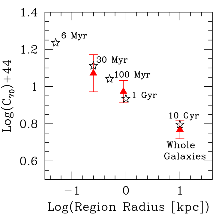
Figure 1: The calibration constant, $C_{70}$, between SFR and the 70 $\mu$m luminosity, expressed as SFR(70)=$C_{70}$ L(70), as a function of the physical size of the regions used to derive the calibration. The filled red triangles are observed values from Li et al. (2010, 2012) and Calzetti et al. (2010), using both Spitzer and Herschel data. The black stars are from stellar population synthesis models, for constant star formation and a Kroupa IMF, in the stellar mass range 0.1–100 $M_{\odot}$; the mean age of the population that best approximates the observed $C_{70}$ values is shown. The scaling between bolometric light and 70 $\mu$m emission is discussed in Calzetti et al. (2010). The association between star formation timescale and region size is based on a region crossing time with a 1–3 km s^-1 speed.

Gas-rich, but metal-poor, galaxies offer little opacity to stellar emission (the same is true for metal-rich, but gas-poor galaxies, e.g., ellipticals, but for these galaxies few or no stars form). Metal content correlates with galaxy luminosity (Tremonti et al. 2004, and references therein), and faint galaxies are faint IR emitters. In this case, SFR(IR) becomes a highly uncertain tool. SFR tracers that mix tracers of both dust-obscured and dust-unobscured star formation have recently been calibrated, and will be presented in Section 2.1.4.

2.1.3 Indicators based on ionised gas emission

Young, massive stars produce copious amounts of ionising photons that ionise the surrounding gas. Hydrogen recombination cascades produce line emission, including the well-known Balmer series lines of H$\alpha$ (0.6563 $\mu$m) and H$\beta$ (0.4861 $\mu$m), which, by virtue of being strong and located in the optical wavelength range, represent the most traditional SFR indicators (Kennicutt 1998).

Only stars more massive than $\sim$20 $M_{\odot}$ produce a measurable ionising photon flux. In a stellar population formed through an instantaneous burst with a Kroupa IMF the ionising photon flux decreases by two orders of magnitude between 5 Myr and 10 Myr after the burst.

The relation between the intensity of a hydrogen recombination line and the ionising photon rate is dictated by quantum mechanics, for a nebula that is optically thick to ionising photons (case B, Osterbrock & Ferland 2006). Case B is usually assumed for most astrophysical situations where SFRs are of interest. Although typical interstellar hydrogen densities are sufficient to ensure that most Hii regions should be radiation-bound, inhomogeneities in the interstellar medium cause some fraction of the ionising photons to leak out of the regions (but usually not out of galaxies). More discussion on this issue is given below. The relation between the luminosity of the H$\alpha$ emission line and the ionising photon rate is given by Osterbrock & Ferland (2006):

$$L({\rm H}\alpha)=\frac{\alpha_{{\rm H}\alpha}^{\rm eff}}{\alpha_{\rm B}}h\nu_{{\rm H}\alpha}Q({\rm H}^{o})=1.37\cdot 10^{-12}\ Q({\rm H}^{o})$$ (8)

where L(H$\alpha$) is in erg s^-1, $\alpha_{{\rm H}\alpha}^{\rm eff}$ is the effective recombination coefficient at H$\alpha$, $\alpha_{\rm B}$ is the case B recombination coefficient, $Q({\rm H}^{o})$ is the ionising photon rate in units of s^-1, and the constant at the right-hand side of the equation is the resulting coefficient for electron temperature $T_{\rm e}$=10000 K and density $n_{\rm e}$=100 cm^-3. For a Kroupa IMF (Section 2.2), the relation between ionising photon rate and SFR is:

$${\rm SFR}(Q({\rm H}^{o}))=7.4\cdot 10^{-54}Q({\rm H}^{o})$$ (9)

with SFR(Q$({\rm H}^{o})$) in $M_{\odot}$ yr^-1. Combining Equations 8 and 9, we obtain the well-known calibration:

$${\rm SFR}({\rm H}\alpha)=5.5\cdot 10^{-42}L({\rm H}\alpha)$$ (10)

again, with SFR(H$\alpha$) in $M_{\odot}$ yr^-1 and L(H$\alpha$) in erg s^-1. The variation of the calibration constant is $\sim$15% for variations in electron temperature in the range $T_{\rm e}$=5000–20000 K , and is $<$1% for electron density variations in the range $n_{\rm e}$=100–10⁶ cm^-3 (Osterbrock & Ferland 2006). Star formation needs to have remained constant over timescales $>$6 Myr for the calibration constant to be applicable (Table 1), but there is no dependency on long timescales, unlike SFR(UV) or SFR(TIR).

All SFR indicators that use the ionisation of hydrogen to trace the formation of massive stars are sensitive to the effects of dust. The most commonly treated effect is that of dust attenuation of the line or continuum. As we will see in Section 4, various techniques have been developed to try to remove this effect; furthermore, dust attenuation decreases for increasing wavelength. A far more difficult effect to treat is the direct absorption of Lyman continuum photons by dust. In this case, the ionising photons are removed altogether from the light beam and are no longer available to ionise hydrogen. Thus, no emission from either recombination lines or free-free continuum emission will result. The actual impact of Lyman continuum photon (Lyc) absorption by dust has been notoriously difficult to establish from an empirical point of view, owing to the absence of a ‘ground truth’ (or reference) with which to compare measurements. Models have to be involved, and these show that the level of Lyc absorption depends on the assumption for the geometry of the nebulae (Dopita et al. 2003, and references therein). The parametrisation of Dopita et al., where the ratio of H$\beta$ line luminosity with and without Lyc absorption is given as a function of the product of metal abundance and ionisation parameter, shows that most normal disk galaxies fall into the regime of low Lyc absorption, typically less than 15%–20%; however, Lyc absorption by dust can become significant at large ionisation parameters and metallicities, such as those typical of local luminous and ultra-luminous IR galaxies (LIRGs and ULIRGs, galaxies with bolometric luminosity $>$ a few 10¹¹ $L_{\odot}$), and of some high-density central regions of galaxies.

A somewhat opposite effect is represented by leakage of ionising photons, i.e., case B recombination does not fully apply. Leakage of ionising photons from galaxies is likely negligible, at the level of a few percent or less (e.g., Heckman et al. 2011), although the jury is still out in the case of low-mass, low-density galaxies (Hunter et al. 2010; Pellegrini et al. 2012). Star-forming regions within galaxies tend, on the other hand, to be leaky, and lose about 25%–40% of their ionising photons (see recent work by Pellegrini et al. 2012; Relaño et al. 2012; Crocker et al. 2012). Thus, the use of ionising photon tracers for local SFRs may be biased downwards by about 1/3 of their true value because of this effect. This correction is not included in Table 1.

Adopting for the moment that Lyc absorption by dust and leakage are not issues, emission lines still need to be corrected for the effects of dust attenuation. As an example, a modest attenuation of $A_{V}$=1 mag by foreground dust depresses the H$\alpha$ luminosity by a factor $\sim$2. At longer wavelengths, Br$\gamma$ (2.16 $\mu$m) is depressed by only 11%, for the same $A_{V}$. Recent advances in the linearity, stability, and field-of-view size of infrared detectors’ are making it possible to collect significant samples of galaxies observed in the IR Hydrogen recombination lines. Table 1 shows a calibration for Br$\gamma$, derived under the same assumptions as SFR(H$\alpha$). Calibrations for other lines can be inferred from those of H$\alpha$ and Br$\gamma$ and the emissivity ratios published in Osterbrock & Ferland (2006).

Recombination lines at wavelengths longer than the optical regime, while offering the advantage of lower sensitivity to dust attenuation, have the dual disadvantage of being progressively fainter and more sensitive to the physical conditions of the gas, especially the temperature; these are natural consequences of transition probabilities and conditions of thermal equilibrium, respectively. The luminosity of Br$\gamma$ is about 1/100th of that at H$\alpha$, and it changes by about 35% for $T_{\rm e}$ in the range 5000–20000 K, and by $\sim$4% for density in the range $n_{\rm e}$=10²–10⁶ cm^-3. For Br$\alpha$ (4.05 $\mu$m), the variations are 58% and 13% for changes in $T_{\rm e}$ and $n_{\rm e}$, respectively. The sensitivity of Br$\gamma$ and Br$\alpha$ to $T_{\rm e}$ is a factor 2.4 and 3.9 larger, respectively, than that of L(H$\alpha$).

New or greatly improved radio and millimetre facilities such as ALMA (the Atacama Large Millimetre/submillimetre Array) or EVLA (the Expanded Very Large Array) are opening the window for exploring millimetre and/or radio recombination lines as ways to measure SFRs unimpeded by effects of dust attenuation, albeit using lines that are intrinsically extremely weak. I will cumulatively refer as RRLs all (sub)millimetre and radio recombination lines from hydrogen quantum levels $n>$20. At high quantum numbers ($n>$80–200, depending on electron density), i.e., at wavelengths of a few cm or longer, stimulated emission is no longer negligible and adds extra parameters in the expression of the line luminosity (Brown et al. 1978). Even within the regime where stimulated emission is not a concern, the line luminosity is dependent on the electron temperature, producing SFR(RRL)$\propto T_{\rm e}^{0.7}$ (Gordon & Sorochenko 2009). This translates into a variation in the line intensity of a factor 2.6 for $T_{\rm e}$ in the range 5000–20000 K.

The traditional approach of measuring the electron temperature from the radio line-to-continuum ratio relies on the assumption that the underlying continuum is free-free emission. The true level of free-free emission from a galaxy, or from a large star-forming region embedded in a galaxy, needs to be carefully disentangled from both dust emission (dominant $<$ 2–3 mm) and synchrotron emission (dominant $>$ 1–3 cm, depending on the source). Often, multi-wavelength observations are used to accomplish this (e.g., Murphy et al. 2011), and add an additional layer of complication to the use of SFR(RRL). Exploratory work is still ongoing to test how efficiently RRLs can be detected in external galaxies (e.g., Kepley et al. 2011), and what advantage they can bring relative to more classical and efficient methods. If the high-density, and heavily dust-obscured, regime turns out to be the main niche for these tracers (Yun 2008), they will need to be carefully weighted against SFR(IR), in light of the potentially heavy impact of the Lyc absorption by dust.

The free-free emission from galaxies or regions itself is a SFR tracer, being the product of the Coulomb interaction between free electrons and ions in thermal equilibrium. The electron temperature dependence of this SFR tracer, SFR(ff)$\propto T_{\rm e}^{-0.45}$ (Condon 1992), is shallower than that of the SFR(RRL), implying less than a factor of two change for a factor of four variation in $T_{\rm e}$. A calibration of SFR(ff) consistent with our IMF choice is given in Murphy et al. (2011).

SFR tracers that use forbidden metal line emission will not be discussed in this review, as they suffer from the same limitations as the hydrogen recombination lines, and have additional dependencies on the metal content and ionisation conditions of a galaxy or region. A review is found in Kennicutt (1998) and a recent calibration in Kennicutt et al. (2009).

2.1.4 Indicators based on mixed processes

The necessity to capture both dust-obscured and dust-unobscured star formation has led to the formulation of SFR indicators that attempt to use the best qualities of each indicator above. This advantage compensates for the slight disadvantage of having to obtain two measures at, generally, two widely separated wavelengths: one that measures the direct stellar light and one that measures the dust-processed light. These mixed indicators have been calibrated empirically over the past $\sim$5–7 years, using combinations of data from space and the ground (e.g., Calzetti et al. 2005, 2007; Kennicutt et al. 2007, 2009; Liu et al. 2011; Hao et al. 2011), and are usually expressed as:

$${\rm SFR}(\lambda_{1},\lambda_{2})=C(\lambda_{1})[L(\lambda_{1})_{\rm obs}+a_{\lambda_{2},{\rm Type}}L(\lambda_{2})_{\rm obs}]$$ (11)

with SFR$(\lambda_{1},\lambda_{2})$ in $M_{\odot}$ yr^-1. $\lambda_{1}$ is usually a wavelength probing either direct stellar light (e.g., the GALEX FUV at 0.153 $\mu$m) or ionised gas tracers (e.g., H$\alpha$), and $\lambda_{2}$ is a wavelength or range of wavelengths where dust emission dominates (e.g., 24 $\mu$m, 25 $\mu$m, TIR, etc.). The constant $C(\lambda_{1})$ is the calibration for the direct stellar light probe, often derived from models (see Table 1). The luminosities $L(\lambda_{1})_{\rm obs}$ and $L(\lambda_{2})_{\rm obs}$ are in units of erg s^-1 and are the observed luminosities (i.e., not corrected for effects of dust attenuation or other effects). The proportionality constant a${}_{\lambda_{2},{\rm Type}}$ depends on both the dust emission tracer used and whether the calibration is for local or global use (Type=local, global). This latter characteristic is due to the sensitivity of dust emission to heating from a wide range of stellar populations (see Section 2.1.2). An example of a mixed indicator calibration is given in Fig. 2.

Table 2: Mixed processes-based SFR calibrations^a

$\lambda_{1}^{b}$	$\lambda_{2}^{b}$	$C_{\lambda_{1}}^{c}$	$a_{\lambda_{2},{\rm Type}}^{d}$	Typed
FUV (0.153 $\mu$m)	24 $\mu$m	4.6$\times$10-44	6.0	local
FUV (0.153 $\mu$m)	25 $\mu$m	4.6$\times$10-44	3.89	global
FUV (0.153 $\mu$m)	TIR	4.6$\times$10-44	0.46	global
H$\alpha$	24 $\mu$m	5.5$\times$10-42	0.031	local
H$\alpha$	25 $\mu$m	5.5$\times$10-42	0.020	global
H$\alpha$	TIR	5.5$\times$10-42	0.0024	global

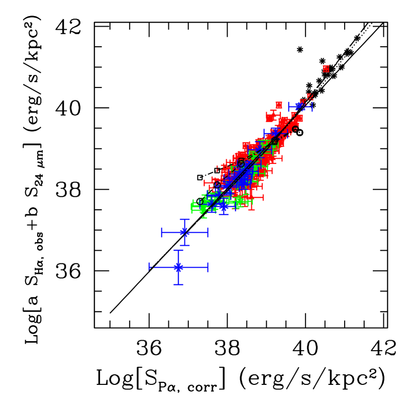
Figure 2: An example of the calibration for a mixed SFR indicator, from Calzetti et al. (2007). This specific example is for a local SFR indicator: the data points include star-forming regions in nearby galaxies (red triangles, green squares, blue crosses) and local LIRGs (black stars, from Alonso-Herrero et al. 2006). The horizontal axis is the luminosity/area of the regions/galaxies in the hydrogen recombination line P$\alpha$ (1.8756 $\mu$m), the vertical axis is a linear combination of the luminosity/area of the observed H$\alpha$ and 24 $\mu$m luminosity. The star-forming regions include low (blue), intermediate (green), and high (red) metallicity. All the points align basically along a one-to-one relation (straight continuous line) suggesting that this calibration is fairly independent of the metallicity (dust content) and luminosity of the source. Other lines mark the position of models as described in Calzetti et al. (2007).

Table 2 summarises a few of the published calibrations from the references above; a more complete set of global calibrations can be found in the recent review by Kennicutt & Evans (2012). Local calibrations show systematically higher values of $a_{\lambda_{2},{\rm Type}}$ than global ones. At 24–25 $\mu$m, $a_{24,{\rm local}}/a_{25,{\rm global}}\sim 1.55$. This difference cannot be attributed to the difference between L(24) and L(25), which is around 2% typically (Kennicutt et al. 2009; Calzetti et al. 2010). The larger fraction of 24 $\mu$m emission that needs to be added to either FUV or H$\alpha$ in local SFR measurements may simply reflect the fact that regions within galaxies are probing stellar populations over shorter timescales ($\tau\sim$100 Myr or smaller) than global SFR measurements ($\tau>$ many Gyr). The dust emission traces this difference accordingly (Kennicutt et al. 2009). From Table 1, the ratio of the calibration constants for SFR(TIR) at 100 Myr and 10 Gyr is 1.75, close to the observed value of 1.55. Differences in the mean dust temperature, that is likely to boost the L(24) in sub-galactic regions, may account for the remaining discrepancy.

2.1.5 Indicators based on other processes

SFR indicators based on non-thermal (synchrotron) radio and X-ray emission represent more indirect ways of probing star formation in galaxies.

In the case of synchrotron emission, the basic mechanism is the production and acceleration of cosmic rays in supernova explosions; since the supernova rate is directly related to the SFR, we should be able to use the synchrotron luminosity as a proxy for the SFR. There is, however, an added complication in that the non-thermal luminosity depends not only on the mean cosmic ray production per supernova, but also on the galaxy’s magnetic field (e.g., Rybicki & Lightman 2004). The case for SFR(sync) is helped by the well-known IR-radio correlation (e.g., Yun et al. 2001): if the IR is correlated with both SFR and radio emission, then SFR and radio emission are correlated among themselves. SFR(sync) calibrations can only be derived empirically (Condon 1992; Schmitt et al. 2006; Murphy et al. 2011), because of the complexity of the relation between the SFR and the underlying physical mechanism; a recent derivation consistent with our IMF can be found in Murphy (2011).

A similarly indirect relation exists between SFR and X-ray luminosity. In star-forming galaxies, the X-ray luminosity is produced by high-mass X-ray binaries, massive stars, and supernovae, but non-negligible contributions from low-mass X-ray binaries are also present. The latter are not directly related to recent star formation, and represent a source of uncertainty in the calibration of SFR(X-ray). Because of the difficulty of establishing the frequency and intrinsic luminosity of each X-ray source (related or unrelated to current star formation) from first principles, the SFR(X-ray) calibrations have been derived empirically, and examples are given in Ranalli et al. (2003), Persic & Raphaeli (2007), and Mineo et al. (2012). Care should be taken when comparing these published calibrations, obtained for a Salpeter IMF, with those reported in this summary, which are based on a Kroupa IMF.

2.2 A word about the stellar initial mass function and
stochastic sampling

All calibrations listed in this section make the implicit assumption that the stellar IMF is constant across all environments and given by the double-power law expression (Kroupa 2001):

$$\chi(M)=dN/dM = A\ M^{-1.3}~{}~{}~{}~{}~{}~{}~{}~{}~{}~{}(0.1\leq M(M_{\odot})\leq 0.5)$$ (12)

$$= 0.5\ A\ M^{-2.3}~{}~{}~{}~{}~{}(0.5\leq M(M_{\odot})\leq 100)$$

where $\chi(M)$ is the number of stars between $M$ and $M+dM$. The stellar mass distribution and total stellar mass produced by this expression are not significantly different from that produced by the log-normal expression proposed by Chabrier (2003). The Kroupa IMF expression produces a smaller number of low-mass stars than the Salpeter (1955) IMF, which has been customarily represented with a single power law with slope $-2.35$ between 0.1 and 100 $M_{\odot}$. Since the majority of SFR indicators trace massive stars, a calibration based on the Kroupa IMF can be converted to one using the Salpeter IMF simply by multiplying the calibration constant by 1.6.

The assumption that the IMF is constant and universal is justified by many observational results, although these are generally rather uncertain, especially at the high-mass end (review by Bastian et al. 2010). There is still the possibility of variation in some extreme (in terms of density, SFR, or other) environments, and arguments both in favour of and against variations have been brought forward by many different authors. To gauge the impact of a different IMF assumption on our SFR calibrations, we can adopt a modified Kroupa IMF, with the maximum stellar mass set to 30 $M_{\odot}$, instead of 100 $M_{\odot}$. The new calibration constants, for selected timescales, are listed in Table 1. The constants change by factors 1.4, 1.5, and 5.6 for SFR(UV), SFR(TIR), and SFR(H$\alpha$), respectively. The change for the H$\alpha$ calibration is the largest of all; it is larger than the UV one by a factor of four, simply because significant UV emission is produced by stars down to $\sim$5 $M_{\odot}$, but significant ionising photon flux is produced only by stars more massive than $\sim$20 $M_{\odot}$. In addition, it takes slightly longer (10 Myr for the upper mass limit of 30 $M_{\odot}$versus 6 Myr for 100 $M_{\odot}$) for the ionising photons to reach their asymptotic value. The changes for the UV and TIR calibration constants are similar to each other.

In contrast with the results just discussed, the mean stellar mass for the Kroupa IMF is $\langle M\rangle$$\sim$0.6 $M_{\odot}$, with less than 10% difference between using 100 $M_{\odot}$ or 30 $M_{\odot}$ as stellar upper mass limit. This makes tracers based on the mean stellar mass of a system (Equation 1) more robust than those based on tracing the most massive stars.

Even if the IMF is universal, individual systems may show departures from this condition, based on simple arguments of sampling.

If we consider a single-age, very young stellar cluster, we can ask what the minimum mass is that this cluster needs to have so that at least one star with mass 100 $M_{\odot}$ is formed. The mass is 2.8$\times$10⁵ $M_{\odot}$, which is a large value, only achieved by some of the most massive star clusters known. As a comparison, if the maximum stellar mass is 30 $M_{\odot}$, full sampling of the IMF, meaning that at least one 30 $M_{\odot}$ star is formed, is achieved with a cluster mass of 1.7$\times$10⁴ $M_{\odot}$.

Under these circumstances, it is not uncommon that studies that involve low SFRs, either because the region considered is small and/or inefficient at forming stars, or because the galaxy has a low overall SFR, are subject to the effects of stochastic sampling, i.e., the stellar IMF is randomly, not fully, sampled. The impact of stochastic sampling is higher for the most massive stars, since there are proportionally less massive stars than low-mass ones. From the Kroupa IMF expression above, only 11% of all stars, by number, have masses above 1 $M_{\odot}$, although these stars represent 56% of the total mass.

Stochastic sampling has a larger impact on tracers of ionising photons than on tracers of UV continuum light, for the same reason that a low upper limit in stellar mass has. Clear evidence for this is shown by the so-called extended UV (XUV) disks of galaxies, as revealed by GALEX. The original hypothesis that these XUV disks, bright in the UV but faint in H$\alpha$, could be due to peculiar IMFs (e.g., deficient in high-mass stars) has been replaced by the finding that the IMF is stochastically sampled in these low-SFR areas (Goddard et al 2010; Koda et al. 2012). The models of Cerviño et al. (2002), renormalised to the Kroupa IMF (Equation 12), show that a star cluster with mass $\sim$1$\times$10⁴ $M_{\odot}$ will be subject to sufficient stochastic sampling that a scatter as large as 20% can be expected in the measured ionising photon flux. The scatter increases dramatically for decreasing cluster mass, and becomes as large as 70% for a cluster mass $\sim$1$\times$10³ $M_{\odot}$. This poses a practical limitation of SFR$\gtrsim$0.001 $M_{\odot}$ yr^-1 for the use of SFR indicators based on the ionising photon flux if a 20% or less uncertainty is desired; a similar uncertainty value for the UV is obtained at SFR$\gtrsim$0.0003 $M_{\odot}$ yr^-1, or about 3.5 times lower than when using tracers of ionising photons (Lee et al. 2009, 2011).

3 The nature of ‘diffuse’ light in galaxies

In the previous sections, I have attempted to discriminate SFR calibrations applicable to whole galaxies from those applicable to regions within galaxies. As already mentioned at the beginning of this chapter, whole galaxies are, in first approximation, isolated systems. As long as they are calibrated and used in a self-consistent manner, most SFR indicators should yield similar values, and reflect the actual rate of recent star formation in a galaxy.

Regions within galaxies, instead, are emphatically not isolated. Most young star clusters disperse quickly (infant mortality due to gas expulsion), and they continue to disperse as they evolve, due to both stellar evolution and a variety of dynamical effects that include two-body relaxation, tidal stripping, large-scale shocks, etc. (Lamers et al. 2010). Models agree that as many as 80%–90% of clusters dissolve within the first 10–20 Myr of life, and their stars become part of the diffuse field, although the same models tend to disagree on the level of evolution at later stages (Fall et al. 2005; Lamers et al. 2005; Chandar et al. 2010). Cluster evolution and dispersal within the first few tens of Myr is what this review is mostly concerned with, since this can influence the derivation and interpretation of local SFRs.

Analysis of the HST UV spectra of star clusters and of the intracluster diffuse stellar light in the starburst regions of nearby galaxies has revealed marked differences between the two stellar populations. Star clusters show clear signatures of the presence of O star wind features, signalling the existence of stars more massive than $\sim$30 $M_{\odot}$ in the clusters. Conversely, the intracluster population systematically lacks those features (Tremonti et al. 2001; Chandar et al. 2005). Sufficient area is covered in each galaxy that stochastic sampling in the diffuse light regions is not an issue. The significant difference in the spectral features of cluster and intracluster spectra excludes the possibility that the intracluster UV light is scattered light which originates from the clusters themselves. Only two scenarios, thus, appear in agreement with the data: (1) stars form locally in the diffuse field, but either they have a different IMF than that of the clusters or they form in small clusters that systematically lack massive stars (Meurer 1995; Weidner et al. 2010); (2) most stars form in clusters, and the clusters dissolve over 7–10 Myr (Tremonti et al. 2001; Chandar et al. 2005).

Option (2) may be the most viable of the two scenarios, in light of what has been discussed earlier in this section. An important consideration is that option (1), also referred to as in-situ star formation, necessarily implies either a different IMF or a different cluster mass function between the clusters and the field.

GALEX has surveyed many local star-forming galaxies in the UV, at 0.153 $\mu$m (FUV) and 0.231 $\mu$m (NUV), across their entire disk. One of the most striking results is that the FUV$-$NUV colours of the arm regions are in general significantly bluer than those of the interarm regions (D. Thilker, private communication), despite the arms usually containing more dust than the interarms, roughly 1 mag more in the $I$-band (White et al. 2000; Holwerda et al. 2005). These red interarm colours, if not attributable to dust reddening, can result from evolving stellar populations that are diffusing from the arm regions (e.g., Pellerin et al. 2007). For example, in the galaxy NGC 300, located only 2 Mpc away, the UV colours are consistent with a dominant interarm population that is devoid of stars younger than 10–20 Myr. Another scenario for the UV light in the interarm regions of disk galaxies is dust-scattered light diffusing from the spiral arms (Popescu et al. 2005), although the significantly redder colours in the interarm regions could pose a challenge to this interpretation. Unambiguous evidence for scattered UV photons by dust has been found in the starburst-driven outflows of the two nearby galaxies M 82 and NGC 253 (Hoopes et al. 2005).

The UV light at 0.16 $\mu$m of a stellar population undergoing constant star formation for the past 100 Myr is contributed for $\sim$70% and $\sim$30% by stars younger and older than 10 Myr, respectively. We assume for simplicity that all stars younger than 10 Myr populate spiral arms, and those older than that are located in the interarm regions. Adopting extinction values of $A_{I}$=1.5 mag and 0.5 mag in the spiral and interarm regions, respectively, as determined by Holwerda et al. (2005), and a very simple dust geometry, the observed 0.16 $\mu$m UV emission becomes 40% and 60% contributed by stars younger and older than 10 Myr, respectively, almost reverting the intrinsic ratios. The observed ratio is about 50%–50% in NGC 5194 and NGC 3521 (Liu et al. 2011). Dust geometry plays a crucial role in this case, and almost about any value of the observed UV fraction from the two components can be obtained by varying the dust geometry, within a reasonable range for the geometrical distributions of dust and stars (see section 4).

Whether due to dust scattering and/or ageing stellar populations diffusing from the spiral arms and/or some in-situ star formation, or a combination of all three, the UV light in the inter-arm regions of spiral galaxies displays a more complex nature than that of the arms. This consideration suggests caution in using standard calibrations of the SFR(UV) in spatially-resolved studies of disks, especially when the targeted regions include inter-arm areas that have not been independently confirmed to be actively star-forming.

The escape of ionising photons from Hii regions has been already discussed in Section 2.1.3. It is at the level of 40%–60% for the observed H$\alpha$ emission (e.g., Ferguson al. 1996; Thilker et al. 2002; Oey et al. 2007), but gets reduced to $\sim$30% when differential extinction in the H$\alpha$ within and outside the Hii regions is accounted for (Crocker et al. 2012). The nature of the diffuse H$\alpha$ in galaxies has been the subject of extensive studies by a number of authors, with still some open questions (e.g., Witt et al. 2010). For the purpose of measuring SFRs, we need to consider two effects. Firstly, the leakage of ionising photons from star-forming regions will impact SFR($Q(H^{o}$)), reducing it roughly by 30% (trends with luminosity, gas density, etc, are only now starting to be investigated, see Pellegrini et al. 2012). Secondly, weak recombination line emission will appear in regions that are not star-forming; in sensitive surveys, this emission could be mistaken for faint in-situ star formation. This second effect should not be underestimated, as ionising photons have been shown to travel as far as about 1 kpc from their point of origin.

The non-discriminating nature of dust in regard to the sources of heating poses another challenge for local SFR measurements, if the IR is used as an indicator, either alone or in combination with a UV/optical one. The UV/optical photons produced by the stellar population of the diffuse field are generally sufficient to heat the dust in a galaxy (Draine et al. 2007). As already mentioned in Section 2.1.2, the 8 $\mu$m emission from a galaxy may be a better tracer of B stars than recent star formation (Boselli et al. 2004; Peeters et al. 2004), and about 30% of the 8 $\mu$m emission from the nearby galaxy NGC 628 is unrelated to star formation more recent than 100 Myr (Crocker et al. 2012). A similar fraction, $\sim$30%, is recovered at 24 $\mu$m, when comparing the local with the global SFR indicators (see Section 2.1.4). Direct attempts to quantify the fraction of 24 $\mu$m emission unrelated to recent star formation provide a minimum conservative value of about 20% (Leroy et al. 2012), with as much as 50% of the emission heated by populations older than $\sim$10 Myr (Liu et al. 2011). Intermediate (0.2–2 Gyr) age stars can be bright in the 20–45 $\mu$m region, significantly contributing to the emission in this wavelength region (Verley et al. 2009; Kelson & Holden 2010).

In a study of the Triangulum Galaxy (M 33), Boquien et al. (2011) identify a threshold of SFR/area=10^-2.75 $M_{\odot}$ yr^-1 kpc^-2, above which the IR emission reliably traces the current SFR; in M 33, this threshold delineates the spiral arms and the central $\sim$1.2 kpc region, and excludes most of the interarm regions, which are dominated by evolved star heating. Dust can also be heated by UV photons leaking out of the arms into the interarm regions (Popescu et al. 2005; Law et al. 2011). In this case, the heating is not produced by in-situ star formation, but by photons that have originated a large distance away. In summary, care should be taken when attempting to measure SFRs in faint galaxy regions using the IR emission, since this emission may be dominated by heating by old stars and/or UV photons leaking out of Hii regions a large distance away, instead of tracing in-situ star formation.

The general conclusion to be taken away from this section is that SFR measurements at any wavelength could be tricky in regions that are not obviously dominated by recent star formation, such as the interarm regions of galaxies.

4 Dust attenuation of the stellar light

4.1 General properties

In this section, I will briefly discuss the effect of dust attenuation on both the stellar continuum and the ionised gas line emission. Because of the complexity of the topic, this section will be incomplete, and the interested reader is referred to the included list of references, and to the review of Calzetti (2001).

I make here the explicit distinction between ‘attenuation’ (minted for such use by Gerhardt Meurer, to my best recollection) and ‘extinction’.

Extinction refers to the combined absorption and scattering (out of the line of sight) of light by dust. The light is provided by a background point source (star, quasar), and the dust is entirely foreground to the source. Because the source is a background point, the distribution of the foreground dust is irrelevant to the total extinction value (left panel of Fig. 3).

Attenuation refers to the net effect of dust in a complex geometrical distribution, where the light sources are distributed within the dust at a range of depths, including in front of and behind it, and the dust itself can be clumpy, smooth, or anything in between. Because both the light sources and the dust have extended distributions, their relative location has a major impact on the net absorbed and scattered light, the latter now including scattering into, as well as out of, the line of sight (right panel of Fig. 3). Dust scattering into the line of sight has the effect of producing a greyer overall attenuation than if only scattering out of the line of sight were present, and the emerging SED will be bluer. This is the typical situation encountered when studying galaxies or extended regions within galaxies.

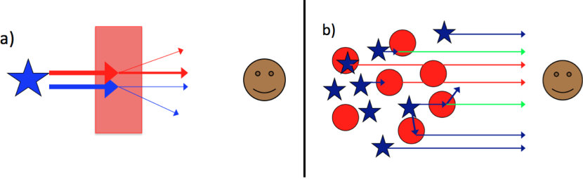
Figure 3: The left (a) and right (b) panels are cartoon representations of: a) a point source (star) behind a screen of dust; and b) an extended distribution of stars mixed with clumps of dust. The left panel shows the typical configuration that enables measures of extinction curves: a single illuminating source located in the background of the dust. The dust extinguishes the light via direct absorption and via scattering out of the line of sight. The right panel is more representative of the situation encountered whenever a complex distribution of stars and dust is present, as found in external galaxies and large regions. In this case, different stars may encounter different numbers of dust clouds (differences in optical depth), and some stars can be entirely embedded in dust (internal extinction) or be completely foreground to the dust distribution. Scattering of the light by dust both into and out of the line of sight is present. Because of the more complex geometrical relation between dust and the illuminating sources, the net effect of dust on the stellar population’s SED is termed attenuation.

The radiative transfer of light through dust is described by an integro-differential equation. At UV/optical/near-IR wavelengths, the radiative transfer equation is:

$$\frac{dI_{\nu}}{d\tau}=-I_{\nu}+\frac{a_{\nu}}{\pi}\int I_{\nu}\phi(\nu,{\rm cos}\ \Theta)d\Omega$$ (13)

where $I_{\nu}$ is the light intensity, $\tau$ is the optical depth through the dust, $a_{\nu}$ is the dust albedo (i.e., the ratio of the scattering coefficient to the sum of the scattering and absorption coefficients), $\phi(\nu,{\rm cos}\ \Theta)$ is the scattering phase function,and $\Theta$ is the angle between the scattered photon and the line of sight. Expressions for both $a_{\nu}$ and $\phi(\nu,{\rm cos}\ \Theta)$ are given in Draine (2003b). In the equation above, we have neglected the source function, i.e., the dust emission, which usually has small values for wavelengths shorter than a few $\mu$m. The first term to the right-hand side of the equation describes the decrease in intensity of the original beam due to passage inside the dust, and the second term is the light added to the beam by scattering into the line of sight.

General solutions to the problem of how to remove the effects of dust from extended systems are not available. One of the first papers to address this issue specifically for galaxies is due to Witt et al. (1992). Since then, many codes have been made available to the community to treat the radiative transfer of the light produced by a stellar population through dust, with the goal of simulating realistic SEDs of galaxies. As many such codes exist, it is impossible to do justice to them all, and I shall avoid injustice by citing none.

For the simple case in which there is a single point-like light source behind a screen of dust, Equation 13 reduces to

$$\frac{dI_{\nu}}{d\tau}=-I_{\nu}$$ (14)

with the well-known solution for the extinction of a stellar spectrum by foreground dust

$$I_{\nu}=I_{\nu}^{o}\ {\rm e}^{-\tau}$$ (15)

where $I_{\nu}^{o}$ is the incident light and

$$\tau_{\lambda}=0.921\ A(\lambda)=0.921\ E(B-V)\ \kappa(\lambda)$$ (16)

is the optical depth, which is related to the extinction curve $\kappa(\lambda)$ through the colour excess $E(B-V)$. The colour excess is a measure of the thickness of the dust layer, while the extinction curve provides a measure of the overall cross-section of dust to light as a function of wavelength. Observational measures of extinction curves have been obtained only for the Milky Way, the Magellanic Clouds, and M 31 (Cardelli et al. 1989; Bianchi et al. 1996; Fitzpatrick 1999; Gordon et al. 2003, 2009), because these are the only galaxies for which individual stars can be isolated and the extinction properties of the dust in front of them determined. For more distant systems, ‘extinction’ measures are more properly ‘attenuation’ measures.

A few other ‘almost’ exact solutions are available for Equation 13, and all of them require replacing the integral on the right-hand side of the equation with some mean or central value, so the equation changes to a pure differential one. Mathis (1972) and Natta & Panagia (1984) provide an expression for the case of internal extinction, which geometrically corresponds to a homogeneous mixture of stars and dust:

$$I_{\nu}=I_{\nu}^{o}\ \frac{1-{\rm e}^{-\tau^{\prime}}}{\tau^{\prime}}$$ (17)

where $\tau^{\prime}$ is an effective optical depth that needs to include the mean effects of scattering into the line of sight (Mathis 1983).

The two cases of foreground dust (screen; Equation 15) and internal dust (homogeneous mixture; Equation 17) are shown in Fig. 4. This cartoon representation uses the same input stellar SED and dust characteristics, including the dust thickness, as described by the colour excess $E(B-V)=0.5$, and the dust extinction curve, which I take to be the standard Milky Way curve with $R_{V}=A_{V}/E(B-V)=3.1$ (e.g., Fitzpatrick 1999). Despite all similarities, the different geometrical relation between stars and dust produces dramatic differences in the output SED, as shown by the two plots to the right hand side of Fig. 4. In general, a foreground screen produces the largest reddening and dimming of all possible dust geometrical configurations. This is a possible choice if the goal is to maximise the impact of dust on a stellar (or other source) SED.

A homogeneous mixture of dust and stars, conversely, produces an almost grey attenuation, with the output SED remaining basically blue even at UV wavelengths. Adding dust to this configuration does not change the shape of the SED in any major way, but mostly dims it. Thus, at UV/optical wavelengths, the SED of a mixed dust/star system will appear very similar to the SED of a dimmer, almost dust-free system. Only a FIR measurement will be able to discriminate among the two systems.

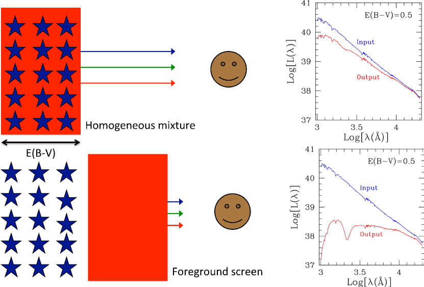
Figure 4: The top and bottom panels show cartoon representations of the same extended distribution of stars and dust, but with a different geometrical relation between each other. In the top panel the dust and stars are homogeneously mixed, while in the bottom panel the dust is completely foreground to the stars. The characteristics of the stars are the same in the two panels. I have assumed that in both cases the dust obeys the Milky Way extinction curve (which has a prominent absorption feature at 2175 Å) with a thickness of $E(B-V)=0.5$. The panels to the right show the input stellar SED, which is the same for the two cases (blue; top spectrum), and the output SED (red; bottom spectrum). All other characteristics being equal, the different geometric relation between dust and stars has considerable impact on the emerging spectrum (‘Output’).

The degeneracy described above is just one of the many degeneracies that are possible when limited information is available on a galaxy SED. A notorious one is the age/dust degeneracy, for which a young, dusty stellar population can have a UV/optical/near–IR SED not dissimilar from that of an old, dust-free population. Breaking of degeneracies usually requires collecting as much information as possible about a system, including, but not limited to, emission line luminosities, the magnitude of the 0.4 $\mu$m break ($D_{\rm n}$(4000), e.g., Kauffmann et al. 2003), and the IR dust luminosity.

A concrete example of how to constrain the dust distribution in a complex system involves the use of hydrogen recombination lines. The intrinsic line-intensity ratio between these lines is set by quantum mechanics, with relatively small variations as a function of electron temperature and density if the lines are at the wavelength of Br$\gamma$ or bluer. Measurements of at least three emission lines, widely spaced in wavelength, probe different dust optical depths, which, when combined, provide strong constrains on the dust geometry, at least up to the longest wavelength probed (e.g., Calzetti 2001). As an example, the three recombination lines H$\beta$ at 0.4861 $\mu$m, P$\beta$ at 1.282 $\mu$m, and Br$\gamma$ probe a factor of ten total difference in optical depth between the bluest and the reddest line, with a factor of four between H$\beta$ and P$\beta$. A common approach when only two lines are available, which most typically are H$\beta$ and H$\alpha$, is to adopt a foreground dust screen, and derive a colour excess by taking the ratio of the observed lines to that of the intrinsic line luminosity as:

$$R_{\alpha\beta}=\frac{[L({\rm H}\alpha)/L({\rm H}\beta)]_{\rm obs}}{[L({\rm H}\alpha)/L({\rm H}\beta)]_{\rm int}}=10^{0.4\ [\kappa({\rm H}\beta)-\kappa({\rm H}\alpha)]\ E(B-V)}$$ (18)

where $\kappa({\rm H}\beta)$ and $\kappa({\rm H}\alpha)$ are the values of the extinction curve evaluated at the wavelength of H$\beta$ and H$\alpha$ ($\kappa({\rm H}\beta)-\kappa({\rm H}\alpha)$=1.163 for the Milky Way extinction curve). Although this approach is rather simplistic, it appears to work reasonably well for local star-forming galaxies, which tend to have modest attenuation values, $A_{V}\sim$1 mag, (Kennicutt 1983; Kennicutt et al. 2009), and for ‘UV-bright starbursts’ (see definition below; Calzetti et al. 1996; Calzetti 2001).

4.2 Application to galaxies

Despite galaxies being difficult to treat in a general fashion, a class of low-redshift galaxies show relatively regular behaviour in their SEDs for increasing dust content. I term these galaxies ‘UV-bright starbursts’, where we use ‘UV-bright’ to discriminate them from LIRGs and ULIRGs: the latter are characterised by a centrally concentrated region of star formation occupying

the inner few hundred parsecs, with 90% or more of their energy output emerging in the IR. We use the term ‘starbursts’ to discriminate them from ‘normal star-forming’ galaxies, these being characterised by widespread star formation across the disk with a relatively low SFR surface density, i.e., such that SFR/area $<$ 0.3–1 $M_{\odot}$ yr^-1 kpc^-2. UV-bright starbursts in the local Universe are galaxies in which the central (inner $\approx$1-2 kpc) starburst dominates the light output at most wavelengths, but which are still sufficiently transparent that a significant fraction of their energy emerges in the UV.

The UV spectral slope, $\beta$, measured in the range $\sim$0.13–0.26 $\mu$m, of local UV-bright starbursts is correlated with the colour excess $E(B-V)$, in the sense that higher values of the colour excess produce redder UV SEDs for these galaxies (Calzetti et al. 1994). The UV spectral slope of these galaxies is also correlated with the infrared excess, measured by the ratio L(TIR)/L(UV) (Meurer et al. 1999); this correlation was termed the IRX-$\beta$ relation by the original authors, where IRX stands for ‘infrared excess’. In recent years, with the wealth of UV imaging data on local galaxies produced by GALEX, it has become customary to replace the UV spectral slope $\beta$ with the UV colour FUV$-$NUV, but the sense of the correlations has remained unchanged. The interpretation of both correlations is straightforward: larger amounts of dust, as traced by the colour excess $E(B-V)$, produce both larger reddening, traced by $\beta$, and larger total attenuations, traced by L(TIR)/L(UV), in the starbursts’ SEDs. The power of such simple correlations, especially the IRX-$\beta$ one, can be immediately appreciated: at high redshift, rest-frame UV spectral slopes are more immediately measurable than total attenuations, since they only require the acquisition of an (observer-frame) optical/near-IR spectrum or colour. The IRX-$\beta$ correlation is, indeed, obeyed by high-redshift starburst galaxies as well (Reddy et al. 2010, 2012).

Two other important characteristics of the dust attenuation trends in local UV-bright starbursts are: (1) the absence of the 0.2175 $\mu$m ‘bump’ (a common feature in the Milky Way extinction curve), which may be an effect of destruction of the carriers; and (2) the fact that the ionised gas emission suffers about twice the attenuation of the stellar continuum (Calzetti et al. 1994). This second characteristic appears to be present also in starburst galaxies at high redshift (e.g., Wuyts et al. 2011).

In terms of dust attenuation, local UV-bright starbursts behave as if the dust were located in a clumpy shell surrounding the starburst region (Calzetti et al. 1994; Gordon et al. 1997; Calzetti 2001). With this simple geometry, dust can be treated as a foreground screen, and the attenuation described as (Calzetti et al. 2000):

$$f_{\rm int}(\lambda)=f_{\rm obs}(\lambda)10^{0.4\ \kappa^{\rm e}(\lambda)\ E(B-V)_{\rm star}}$$ (19)

where $\kappa^{\rm e}(\lambda)$ is an effective attenuation curve to be applied to the observed stellar continuum SED $f_{\rm obs}(\lambda)$ of a starburst galaxy to recover the intrinsic SED $f_{\rm int}(\lambda)$, and with expression:

$$\kappa^{\rm e}(\lambda) = 2.659\ (-1.857+1.040/\lambda)+4.05~{}~{}~{}~{}(0.63\,\mu{\rm m}\leq\lambda\leq 2.20\,\mu{\rm m})$$ (20)

$$= 2.659\ (-2.156+1.509/\lambda-0.198/\lambda^{2}+0.011/\lambda^{3})+4.05$$

$$~{}~{}~{}~{}~{}~{}~{}~{}~{}~{}~{}~{}~{}~{}~{}~{}~{}~{}~{}~{}~{}~{}~{}~{}~{}~{}~{}~{}~{}~{}~{}~{}~{}~{}~{}~{}~{}~{}~{}(0.12\,\mu{\rm m}\leq\lambda<0.63\,\mu{\rm m})$$

and $E(B-V)_{\rm star}$ is the stellar continuum colour excess, which is smaller than that of the ionised gas, as follows:

$$E(B-V)_{\rm star}=0.44\ E(B-V)_{\rm gas}$$ (21)

$E(B-V)_{\rm gas}$ is the same as the $E(B-V)$ in Equation 18.

In the same spirit, the IRX-$\beta$ relation has been given as (Meurer et al. 1999; Calzetti 2001):

$${\rm log_{10}}\biggl{[}\frac{1}{1.68}\biggl{(}\frac{L({\rm TIR})}{L({\rm UV})}\biggr{)}+1\biggr{]}=0.84(\beta-\beta_{\rm o})$$ (22)

where L(UV) is centred around 0.15–0.16 $\mu$m, and $\beta_{\rm o}$ is the intrinsic (unattenuated) UV slope of the galaxies, with typical values $\beta_{\rm o}\sim-2.2$ to $-2.3$, for constant star formation. An example of Equation 22 is given in Fig. 5, together with the data originally used to derive it.

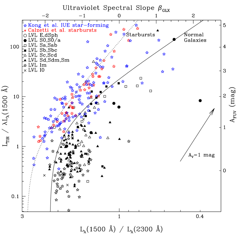
Figure 5: The IRX-$\beta$ plot for local starburst and star-forming galaxies, from Dale et al. (2009). The vertical axis is the IR excess over the UV, where the UV is the GALEX FUV (0.15 $\mu$m) band. The horizontal axis is the GALEX FUV$-$NUV colour, expressed as luminosity ratio, with the corresponding values of the UV spectral slope $\beta$ shown at the top of the plot. The red points are the UV-bright starburst galaxies used by Meurer et al. (1999) to derive the IRX-$\beta$ relation, shown by the dotted line (Equation 22). The blue and black points give the location of normal star-forming galaxies from samples of the local Universe. These galaxies have a much larger spread in the IRX-$\beta$ plane than the UV-bright starbursts, and typically lower IR excesses at constant UV slope. Their mean trend is shown by the continuous line. An A_V=1 mag attenuation vector is also shown. Reproduced with permission from Dale et al. (2009).

Deviations from the simple foreground geometry that can be used for UV-bright starbursts were noted as soon as additional classes of galaxies started to be investigated for systematic trends with dust attenuation. Local LIRGS and ULIRGs, for instance, mostly fall above the locus defined by Equation 22 in the IRX versus $\beta$ plot (e.g., Goldader et al. 2002): typically these galaxies have large IR excesses for their UV slopes. The same trend is observed in high-redshift ULIRGs (Reddy et al. 2010). Geometries that can account for this behaviour include shells of scattering dust and clumps (Calzetti 2001), which can be realised if the dust is located in close proximity to the heating sources, as would be the case in the high-density central regions of the IR-luminous galaxies.

Normal star-forming galaxies, as defined above, also deviate from the locus defined by Equation 22, as do star-forming regions within these galaxies. They generally tend to be located below the starburst curve, i.e., to have low IR excesses for their UV colours, and to have a large spread, about a factor 5–10 larger than the UV-bright starbursts (Fig. 5). This trend has been reported by a large number of authors who have analysed samples of local galaxies and regions within galaxies (Buat et al. 2002, 2005; Gordon et al. 2004; Kong et al. 2004; Calzetti et al. 2005; Seibert et al. 2005; Boissier et al. 2007; Dale et al. 2009; Boquien et al. 2009, 2012). Similar deviations have been reported also for some high-redshift galaxies (Reddy et al. 2012). The interpretation for both the shift towards lower IR excesses and the larger spread than starbursts varies from author to author, and includes: (1) a range of ages in the dominant UV populations; (2) scatter and variations in the dust geometry and composition; or (3) a combination of both. Perhaps, the third interpretation may ultimately be the correct one. Unlike starbursts, in which a more or less causally connected region dominates the energy output, normal star-forming galaxies are a collection of unconnected star-forming regions, each with its own dust geometry and mean age, amid an evolving, but not necessarily UV-faint, diffuse stellar population (Calzetti 2001). In such systems, the UV colour, which has the smallest leverage by covering the shortest wavelength range, will be very sensitive to influences from stellar populations and dust geometry variations (e.g., Kong et al. 2004; Calzetti et al. 2005; Boquien et al. 2009; Hao et al. 2011). Whether one or the other factor predominates, and under which conditions, is still subject of investigation, and it would be premature to provide here a definite answer.

5 Lessons learned

In line with the rest of this chapter, I will summarise the lessons learned on SFR indicators by separating the global, whole-galaxies case from the one describing local, sub-galactic regions.

5.1 Global SFR indicators

As the integrated light from galaxies is a weighted average of the most luminous contributors (i.e., star-forming regions), it is perhaps not surprising that global SFR indicators show a high level of consistency, as summarised in Kennicutt & Evans (2012). As long as the assumptions for the stellar IMF are factored in the calibration constant, stochastic sampling of the IMF is not an issue, and both the dust-obscured and dust-unobscured star formation are accounted for, different SFR indicators should yield similar answers.

All other conditions being equal, SFR indicators that are sensitive only to short timescales, i.e., only probe the presence of short-lived, massive stars, should be preferred to long-timescale ones. Examples of short-timescale SFR indicators are those using ionised gas tracers (e.g., H$\alpha$). Conversely, the IR probes emission from stellar populations covering a large range of ages, and its use will depend on the dominant stellar population contributing to the IR emission and on the required accuracy for the SFR measure: as shown in Table 1, the calibration constant changes by a factor of 1.75 if the timescale of the star formation changes from 100 Myr (e.g., a LIRG or more luminous galaxy) to 10 Gyr (a normal star-forming galaxy).

At high attenuation values, which generally correspond to high SFR values, about a few times 10 $M_{\odot}$ yr^-1 or above, the dust starts competing with the gas for Lyman continuum photon absorption. Combining an ionised gas tracer (e.g., H$\alpha$) with a dust emission tracer (e.g., 24 $\mu$m) is likely to not only mitigate this problem, but also provide a general answer to the question of how to correct UV/optical tracers for the effects of dust attenuation. Mixed SFR indicators (H$\alpha+$24 $\mu$m, UV$+$24 $\mu$m, etc.) have, indeed, broad applicability in all cases where stochastic IMF sampling is not a concern.

At low SFR values, below $\sim$10^-3 $M_{\odot}$ yr^-1, stochastic sampling of the IMF affects the use of ionised gas tracers as SFR indicators. The longer-lived UV emission may thus become a preferable choice, as long as it is corrected for the effects of dust attenuation. Even the UV, however, is not a ‘panacea’, since stochastic IMF sampling starts affecting the UV emission barely a factor three to four below the SFR level of the ionised gas.

Exclusive use of the UV (even after dust attenuation corrections) may complicate the discrimination between star-forming galaxies and post-star-forming galaxies (e.g., Weisz et al. 2012), i.e., galaxies whose active star formation terminated many tens of Myr ago and for which the use of any of the calibration constants in Table 1 will only yield a lower limit.

5.2 Local SFR indicators

Unlike whole galaxies, regions within galaxies are not isolated systems, and a variety of issues needs to be considered when attempting to convert any luminosity into a SFR. Evolution and mixing of stellar populations and the ability of stellar continuum light and ionising photons to leak out of star-forming regions and travel to distances of 1 kpc, and possibly more, are important effects that need to be taken into account for deriving local SFRs. Most of the problems do not reside with the regions of star formation proper, but with the faint regions that may have little or no in-situ star formation. These cumulatively termed ‘non-in-situ star formation’ regions can still emit at many wavelengths, including H$\alpha$, because of leakage from surrounding areas.

The different estimates on the importance of these effects that can be found in the literature (e.g., more than a factor of two difference between Liu et al. 2011 and Leroy et al. 2012) attest to the complexity of the issue. An example of the problems induced by inaccurate estimates of local SFRs is given in Calzetti et al. (2012). Here, it is shown that the relation between the SFR and cold gas surface densities, also known as, the Schmidt-Kennicutt law, strongly depends on the treatment of the ‘non-in-situ’ star formation.

A safe approach, at least for now, is to measure SFRs only in regions where there is ample independent evidence that star formation is actually occurring, such as in spiral arms and in the central regions of many galaxies. The study of M 33 has shown that dust heating is mainly powered by recent star formation in these locales, down to SFR/area$\sim$0.002 $M_{\odot}$ yr^-1 kpc^-2 (Boquien et al. 2011).

Even when star-forming regions or areas have been identified, care should be taken with how the different SFR indicators are applied: the one to choose for a specific case may depend on the star formation timescale of interest. In general, the shorter the timescale, the lower the dependence of the SFR indicator on the evolution of the stellar population. Ionising photon tracers may ‘fit the bill’, although leakage of ionising photons out of star-forming regions will need to be accounted for.

Acknowledgments

I am extremely grateful to the organisers of this Winter School, Johan Knapen and Jesus Falcón-Barroso, for inviting me and for the opportunity to deliver these lectures. I am also grateful to the Instituto de Astrofísica de Canarias and its Director, Prof. Francisco Sánchez, for the hospitality. Many of the results presented in this manuscript are the products of the SINGS (Spitzer Infrared Nearby Galaxies Survey), KINGFISH (Key Insights in Nearby Galaxies: a Far Infrared Survey with Herschel), and LVL (Local Volume Legacy) collaborations, to whose members I am profoundly indebted.

I also want to thank my long-time, long-distance collaborator Robert C. Kennicutt; scientific discussions with him are always enlightening. We often end up with friendly disagreements, and both of our healths have benefited from never residing closer than about 2000 km from each other. Finally, parts of this manuscript have been improved thanks to discussions with another long-time collaborator, John S. Gallagher.

The preparation of this manuscript was supported in part by the NASA-ADAP grant NNX10AD08G and in part by the NASA Herschel grant JPL-1369560 to the University of Massachusetts.

References

- [1] Alonso-Herrero, A., Rieke, G.H., Rieke, M.J. et al. (2006), ApJ, 650, 835
- [2] Aniano, G., Draine, B.T., Calzetti, D. et al. (2012), ApJ, submitted
- [3] Bastian, N., Covey, K.R., & Meyer, M.R. (2010), ARA&A, 48, 339
- [4] Bell, E.F. (2003), ApJ, 586, 794
- [5] Bendo, G.J., Draine, B.T., Engelbracht, C.W. et al. (2008), MNRAS, 389, 629
- [6] Bianchi, L., Clayton, G. C., Bohlin, R. C., Hutchings, J. B., and Massey, P. (1996), ApJ, 471, 203
- [7] Boissier, S., Gil de Paz, A., Boselli, A. et al. (2007), ApJS, 173, 524
- [8] Boissier, S., and Prantzos, N. (2009), A&A, 503, 137
- [9] Boquien, M., Buat, V., Boselli, A. et al. (2012), A&A, 539, A145
- [10] Boquien, M., Calzetti, D., Kennicutt, R.C. et al. (2009), ApJ, 606, 553
- [11] Boquien, M., Calzetti, D., Kramer, C. et al. (2010), A&A, 518, L70
- [12] Boquien, M., Calzetti, D., Combes, F. et al. (2011), AJ, 142, 111
- [13] Boselli, A., Lequeux, J., and Gavazzi, G. (2004), A&A, 428, 409
- [14] Bouwens, R.J., Illingworth, G.D., Franx, M. et al. (2009), ApJ, 705, 936
- [15] Bouwens, R.J., Illingworth, G.D., Oesch, P.A. et al. (2010), ApJ, 709, L133
- [16] Brown, R.L., Lockman, F.J., and Knapp, G.R. (1978), ARA&A, 16, 445
- [17] Buat, V., Boselli, A., Gavazzi, G., and Bonfanti, C. (2002), A&A, 383, 801
- [18] Buat, V., Iglesias-Páramo, J., Seiber, M. et al. (2005), ApJ, 619, L51
- [19] Calzetti, D. (2001), PASP, 113, 1449
- [20] Calzetti, D., Armus, L., Bohlin, R.C. et al. (2000), ApJ, 533, 682
- [21] Calzetti, D., Harris, J., Gallagher, J.S. et al. (2004), AJ, 127, 1405
- [22] Calzetti, D., Kennicutt, R.C., Bianchi, L. et al. (2005), ApJ, 633, 871
- [23] Calzetti, D., Kennicutt, R.C., Engelbracht, C.W. et al. (2007), ApJ, 666, 870
- [24] Calzetti, D., Kinney, A. L., and Storchi-Bergmann, T. (1994), ApJ, 429, 582
- [25] Calzetti, D., Kinney, A. L., and Storchi-Bergmann, T. (1996), ApJ, 458, 132
- [26] Calzetti, D., Liu, G., and Koda, J. (2012), ApJ, in press (astroph/1204.5659)
- [27] Calzetti, D., Wu, S.-Y., Hong, S. et al. (2010), ApJ, 714, 1256
- [28] Cardelli, J. A., Clayton, G. C., and Mathis, J.S. (1989), ApJ, 345, 245
- [29] Cerviño, M., Valls-Gabaud, D., Luridiana, V., and Mass-Hesse, J.M. (2002), A&A, 381, 51
- [30] Chabrier, G. 2003, PASP, 115, 763
- [31] Chandar, R., Leitherer, C., Tremonti, A.C. et al. (2005), ApJ, 628, 210
- [32] Chandar, R., Whitmore, B.C,, Kim, H. et al. (2010), ApJ, 719, 966
- [33] Chomiuk, L., and Povich, M.S. (2011), AJ, 142, 197
- [34] Condon, J.J. (1992), ARA&A, 30, 575
- [35] Crocker, A.F., Calzetti, D., Thilker, D.A. et al. (2012), ApJ, submitted
- [36] Dale, D.A., Cohen, S.A., Johnson, L.C. et al. (2009), ApJ, 703, 517
- [37] Dale, D.A., and Helou, G. (2002), ApJ, 576, 159
- [38] Dole, H., Lagache, G., Puget, J.-L. et al. (2006), A&A 451, 417
- [39] Donas, J., and Deharveng, J.-M. (1984), A&A, 140, 325
- [40] Dopita, M.A., Groves, B.A., Sutherland, R.S., and Kewley, L.J. (2003), ApJ, 583, 727
- [41] Draine, B.T. (2003), ARA&A, 41, 241
- [42] Draine, B.T. (2003b), ApJ, 598, 1017
- [43] Draine, B.T. (2009), in Cosmic Dust - Near and Far, ASP Conference Series, eds. T. Henning, E. Grün, & J. Steinacker. San Francisco, CA: ASP. Vol. 41, 241
- [44] Draine, B.T., Dale, D.A., Bendo, G. et al. (2007), ApJ, 633, 866
- [45] Draine, B.T., and Li A. (2007), ApJ, 657, 810
- [46] Elbaz, D., Dickinson, M., Hwang, H.S. et al. (2011), A&A, 533, A119
- [47] Engelbracht, C.W., Gordon, K.D., Rieke, G.H. et al. (2005), ApJ, 628, 29
- [48] Engelbracht, C.W., Rieke, G.H., Gordon, K.D. et al. (2008), ApJ, 685, 678
- [49] Evans, N.J., Dunham, M.M., Jorgensen, J.K. et al. (2009), ApJS, 181, 321
- [50] Fall, S.M., Chandar, R., and Whitmore, B.C. (2005), ApJ, 631, L133
- [51] Ferguson, A.M.N., Wyse, R.F.G., Gallagher, J.S., and Hunter, D.A. (1996), AJ, 111, 2265
- [52] Fitzpatrick, E.L. (1999), PASP, 111, 63
- [53] Galliano, F., Dwek, E., and Chanial, P. (2008), ApJ, 672, 214
- [54] Giavalisco, M., Dickinson, M., Ferguson, H.C. et al. (2004), ApJ, 600, L103
- [55] Goddard, Q.E., Kennicutt, R.C., and Ryan-Weber, E.V. (2010), MNRAS, 405, 2791
- [56] Goldader, J.D., Meurer, G.R., Heckman, T.M. et al. (2002), ApJ, 568, 651
- [57] Gordon, K.D., Calzetti, D., and Witt, A.N. (1997), ApJ, 487, 625
- [58] Gordon, K.D., Cartledge, S., and Clayton, G.C. (2009), ApJ, 705, 1320
- [59] Gordon, K.D., Clayton, G.C., Misselt, K.A., Landolt, A.U., and Wolff, M.J. (2003), ApJ, 594, 279
- [60] Gordon, K.D., Engelbracht, C.W., Rieke, G.H. et al (2008), ApJ, 682, 336
- [61] Gordon, K.D., Pérez-González, P.G., Misselt, K.A. et al. (2004), ApJS, 154, 215
- [62] Gordon, M.A., and Sorochenko, R.L. (2009), Radio Recombination Lines, Their Physics and Astronomical Applications, Astrophysics and Space Science Library 282, (New York (NY): Springer ScienceBusiness Media
- [63] Gutermuth, R.A., Pipher, J.L., Megeath, S.T. et al. (2011), ApJ, 739, 84
- [64] Hao, C.-N., Kennicutt, R.C., Johnson, B.D. et al. (2011), ApJ, 741, 124
- [65] Heckman, T.M., Borthakur, S., Overzier, R. et al. (2011), ApJ, 730, 5
- [66] Heiderman, A., Evans, N., Allen, L.E., Huard, T., and Heyer, M. (2010), ApJ, 723, 1019
- [67] Helou, G. (1986), ApJ, 311, L33
- [68] Holwerda, B.,W., González, R.A., Allen, R.J., and van der Kruit, P.C. (2005), AJ, 129, 1396
- [69] Hong, S., Calzetti, D., Dopita, M.A. et al. (2011), ApJ, 731, 45
- [70] Hoopes, C.G., Heckman, T.M., Strickland, D.K. et al. (2005), ApJ, 619, L99
- [71] Hopkins, A.M., Connolly, A.J., Haarsma, D.B., and Cram, L.E. (2001), AJ, 122, 288
- [72] Hunter, D.A., Elmegreen, B.G., and Ludka, B.C. (2010), AJ, 139, 447
- [73] Kauffmann, G., Heckman, T.M., White, S.D.M. et al. (2003), MNRAS, 341, 33
- [74] Kelson, D.D., and Holden, B.P. (2010), ApJ, 713, 28
- [75] Kennicutt, R.C. (1983), Apj, 272, 54
- [76] Kennicutt, R.C. (1998), ARA&A, 36, 189
- [77] Kennicutt, R.C. and Evans, N.J. (2012), ARA&A, in press (astroph/1204.3552)
- [78] Kennicutt, R.C., Calzetti, D., Walter, F. et al. (2007), ApJ, 671, 333
- [79] Kennicutt, R.C., Hao, C., Calzetti, D. et al. (2009), ApJ, 703, 1672
- [80] Kepley, A.A., Chomiuk, L., Johnson, K.E. et al. (2011), ApJ, 739, L24
- [81] Kewley, L.J., Geller, M.J., Jansen, R.A., and Dopita, M.A. (2002), AJ, 124, 3135
- [82] Kewley, L.J., Geller, M.J., and Jansen, R.A. (2004), AJ, 127, 2002
- [83] Koda, J., Yagi, M., Boissier, S. et al. (2012), ApJ, 749, 20
- [84] Kong, X., Charlot, S., Brinchmann,J., and Fall, S.M. (2004), MNRAS, 349, 769
- [85] Kroupa, P. (2001), MNRAS, 322, 231
- [86] Lamers, H.J.G.L.M., Baumgardt, H., and Gieles, M. (2010), MNRAS, 409, 305
- [87] Lamers, H.J.G.L.M., Gieles, M., and Portegies, Z.S.F. (2005), A&A, 429, 173
- [88] Law, K.-H., Gordon, K.D., and Misselt, K.A. (2011), ApJ, 738, 124
- [89] Lawton, B., Gordon, K.D., Babler, B. et al. (2010), ApJ, 716, 453
- [90] Lee, Janice C., Gil de Paz, A., Tremonti, C. et al. (2009), ApJ, 706, 599
- [91] Lee, Janice C., Gil de Paz, A., Kennicutt, R.C. et al. (2011), ApJS, 192, 6
- [92] Lee, S.-K., Ferguson, H.C., Somerville, R.S., Wiklind, T., and Giavalisco, M. (2010), ApJ, 725, 1644
- [93] Le Floc’h, E., Papovich, C., Dole, H. et al. (2005), ApJ, 632, 169
- [94] Leitherer, C., Schaerer, D., Goldader, J.D. et al. (1999), ApJS, 123, 3
- [95] Leroy, A.K., Bigiel, F., de Block, W.J.G. et al. (2012), AJ, in press (astroph/1202.2873
- [96] Li, Y., Calzetti, D., Kennicutt, R.C. et al. (2010), ApJ, 725, 677
- [97] Li, Y., Crocker, A.F., Calzetti, D. et al. (2012), in preparation
- [98] Liu, G., Koda, J., Calzetti, D., Fukuhara, M., and Momose, R. (2011), ApJ, 735, 63
- [99] Madden, S.C. (2000), in Massive Stellar Clusters, eds. A Lançon & C. Boily, ASP Conference Series, Vol. 211, 297
- [100] Madden, S.C., Galliano, F., Jones, A.P., and Sauvage, M. (2006), A&A, 446, 877
- [101] Magnelli, B., Elbaz, D., Chary, R.R. et al. (2009), A&A, 496, 57
- [102] Marble, A.R., Engelbracht, C.W., van Zee, L. et al. (2010), ApJ, 715, 506
- [103] Mathis, J.S. (1972), ApJ, 176, 651
- [104] Mathis, J.S. (1983), ApJ, 267, 119
- [105] Meurer, G.R. (1995), Nature, 375, 742
- [106] Meurer, G. R., Heckman, T. M., and Calzetti, D. (1999), ApJ, 521, 64
- [107] Mineo, S., Gilfanov, M., and Sunyaev, R. (2012), MNRAS, 419, 2095
- [108] Moustakas, J., Kennicutt, R.C., and Tremonti, C.A. (2006), ApJ, 642, 775
- [109] Muñoz-Mateos, J.C., Gil de Paz, A., Boissier, S. et al. (2009), ApJ, 701, 1965
- [110] Murphy, E.J., Condon, J.J., Schinnerer, E. et al. (2011), ApJ, 737, 67
- [111] Murphy, E.J., Chary, R.-R., Dickinson, M. et al. (2011b), ApJ, 732, 126
- [112] Natta, A., and Panagia, N. (1984), ApJ, 287, 228
- [113] Oey, M.S., Meurer, G.R., Yelda, S. et al. (2007), ApJ, 661, 801
- [114] Osterbrock, D.E., and Ferland, G.J. (2006), Astrophysics of Gaseous Nebulae and Active Galactic Nuclei, 2nd edition (Sausalito (CA): University Science Books)
- [115] Peeters, E., Spoon,H.W.W., and Tielens, A.G.G.M. (2004), ApJ, 613, 986
- [116] Pellegrini, E.W., Oey, M.S., Winkler, P.F., Points, S.D., and Smith, R.C. (2012), ApJ, in press (astroph/1202.3334)
- [117] Pellerin, A., Meyer, M., Harris, J., and Calzetti, D. (2007), ApJ, 658, L87
- [118] Pérez-González, P.G., Kennicutt, R.C., Gordon, K.D. et al. (2006), ApJ, 648, 987
- [119] Persic, M., and Rephaeli, Y. (2007), A&A, 463, 481
- [120] Pflamm-Altenburg, J., Weidner, C., and Kroupa, P. (2009), MNRAS, 395, 394
- [121] Popescu, C.C., Tuffs, R.C., Madore, B.F., et al., 2005, ApJ, 619, L75
- [122] Ranalli, P., Comastri, A., and Setti, G. (2003), A&A, 399, 39
- [123] Reddy, N.A., Dickinson, M., Elbaz, D. et al. (2012), ApJ, 744, 154
- [124] Reddy, N.A., Erb, D.K., Pettini, M., Steidel, C.C., and Shapley, A.E. (2010), ApJ, 712, 1070
- [125] Relaño, M., Lisenfeld, U., Pérez-González, P.G., Vílchez, J.M., and Battaner, E. (2007), ApJ, 667, L141
- [126] Relaño, M., Kennicutt, R.C., Eldridge, J.J., Lee, J.C., and Verley, S. (2012), MNRAS, in press (astroph/1204.4502)
- [127] Rieke, G.H., Alonso-Herrero, A., Weiner, B.J. et al. (2009), ApJ, 692, 556
- [128] Rosa-González, D., Burgarella, D., Nandra, K. et al. (2007), MNRAS, 379, 357
- [129] Rybicki, G.B., and Lightman, A.P. (2004), Radiative Processes in Astrophysics, 2nd edition (Weinheim (Germany): Wiley-VCH, Verlag)
- [130] Salim, S., Rich, M.R., Charlot, S. et al. (2007), ApJS, 173, 267
- [131] Salpeter, E.E. (1955), ApJ, 121, 161
- [132] Schmitt, H.R., Calzetti, D., Armus, L. et al. (2006), ApJ, 643, 173
- [133] Seibert, M., Martin, D.C., Heckman, T.M. et al. (2005), ApJ, 619, L23
- [134] Smith, J.D.T., Draine, B.T., Dale, D.A. et al. (2007), ApJ, 656, 770
- [135] Sullivan, M., Mobasher, B., Chan, B. et al. (2001), ApJ, 558, 72
- [136] Thilker, D.A., Walterbos, R.A.M., Braun, R., and Hoopes, C.G. (2002), ApJ, 124, 3118
- [137] Tremonti, C.A., Calzetti, D., Leitherer, C., and Heckman, T.M. (2001), ApJ, 555, 322
- [138] Tremonti, C.A., Heckman, T.M., Kauffmann, G. et al. (2004), ApJ, 613, 898
- [139] Treyer, M., Schiminovich, D., Johnson, B.D. et al. (2010), ApJ, 719, 1191
- [140] Verley, S., Corbelli, E., Giovanardi, C., and Hunt, L.K. (2009), A&A, 493, 453
- [141] Verley, S., Relaño, M., Kramer, C. et al. (2010), A&A, 518, L68
- [142] Walter, F., Decarli, R., Carilli, C. et al. (2012), ApJ, in press (astroph/1204.3426)
- [143] Wang, B., and Heckman, T.M. (1996), ApJ, 457, 645
- [144] Weidner, C., Kroupa, P., and Bonnell, I.A.D. (2010), MNRAS, 401, 275
- [145] Weisz, D.R., Johnson, B.D., Johson, L.C. et al. (2012), ApJ, 744, 44
- [146] White, R.E., Keel, W.C., and Conselice, C.J. (2000), ApJ, 542, 761
- [147] Wilkins, S.M., Hopkins, A.M., Trentham, N., and Tojeiro, R. (2008), MNRAS, 391, 363
- [148] Wilkins, S.M., Bunker, A.J., Stanway, E., Lorenzoni, S., and Caruana, J. (2011), MNRAS, 417, 717
- [149] Witt, A.N., Gold, B., Barnes, F.S. et al. (2010), ApJ, 724, 1551
- [150] Witt, A.N., Thronson, H.A., and Capuano, J.M. (1992), ApJ, 393, 611
- [151] Wu, H., Cao, C., Hao, C.-N., et al. (2005), ApJ, 632, L79
- [152] Wuyts, S., Förster-Schreiber, N., Lutz, D. et al. (2011), ApJ, 738, 106
- [153] Yun, M.S. (2008), Ap&SS, 313, 253
- [154] Yun, M.S., Reddy, N.A., and Condon, J.J. (2001), ApJ, 554, 803
- [155] Zhu, Y., Wu, H., Cao, C., and Li, H.-N. (2008), ApJ, 686, 155