Critical phenomena in exponential random graphs

Abstract.

The exponential family of random graphs is one of the most promising class of network models. Dependence between the random edges is defined through certain finite subgraphs, analogous to the use of potential energy to provide dependence between particle states in a grand canonical ensemble of statistical physics. By adjusting the specific values of these subgraph densities, one can analyze the influence of various local features on the global structure of the network. Loosely put, a phase transition occurs when a singularity arises in the limiting free energy density, as it is the generating function for the limiting expectations of all thermodynamic observables. We derive the full phase diagram for a large family of 3-parameter exponential random graph models with attraction and show that they all consist of a first order surface phase transition bordered by a second order critical curve.

1. Introduction

The exponential family of random graphs is one of the most widely studied network models. Their popularity lies in the fact that they capture a wide variety of common network tendencies, such as connectivity and reciprocity, by representing a complex global structure through a set of tractable local features. The theoretical foundations for these models were originally laid by Besag [1], who applied methods of statistical analysis and demonstrated the powerful Markov-Gibbs equivalence (Hammersley-Clifford theorem [2]) in the context of spatial data. Building on Besag’s work, further investigations quickly followed. Holland and Leinhardt [3] derived the exponential family of distributions for networks in the directed case. Frank and Strauss [4] showed that the random graph edges form a Markov random field when the local network features are given by counts of various triangles and stars. Newer developments are summarized in Snijders et al. [5] and Rinaldo et al. [6]. (See Wasserman and Faust [7] for a comprehensive review of the methods and models for analyzing network properties.)

As usual in statistical physics, we start with a finite probability space, namely the set $\mathcal{G}_{n}$ of all simple graphs on $n$ vertices (“simple” means undirected, with no loops or multiple edges). The general $k$-parameter family of exponential random graphs is defined by assigning a probability mass function $\mathbb{P}_{n}^{\beta}(G_{n})$ to every simple graph $G_{n}\in\mathcal{G}_{n}$:

$$\mathbb{P}_{n}^{\beta}(G_{n})=\exp\left(n^{2}(\beta_{1}t(H_{1},G_{n})+\cdots+\beta_{k}t(H_{k},G_{n})-\psi_{n}^{\beta})\right),$$ (1)

where $\beta=(\beta_{1},...,\beta_{k})$ are $k$ real parameters, $H_{1},...,H_{k}$ are pre-chosen finite simple graphs (in particular, we take $H_{1}$ to be a single edge), $t(H_{i},G_{n})$ is the density of graph homomorphisms (the probability that a random vertex map $V(H_{i})\to V(G_{n})$ is edge-preserving),

$$t(H_{i},G_{n})=\frac{|\text{hom}(H_{i},G_{n})|}{|V(G_{n})|^{|V(H_{i})|}},$$ (2)

and $\psi_{n}^{\beta}$ is the normalization constant (free energy density),

$$\sum_{G_{n}\in\mathcal{G}_{n}}\exp\left(n^{2}\left(\beta_{1}t(H_{1},G_{n})+\cdots+\beta_{k}t(H_{k},G_{n})\right)\right)=\exp\left(n^{2}\psi^{\beta}_{n}\right).$$ (3)

These exponential random graphs are particularly useful when one wants to simulate observed networks as closely as possible, but without going into details of the specific process underlying network formation. Since real-world networks are often very large in size, ranging from hundreds to billions of vertices, our main interest will be in the behavior of the exponential random graph $G_{n}$ in the large $n$ limit. Intuitively, the $k$ parameters $\beta_{1},...,\beta_{k}$ allow one to adjust the influence of different local features (in this case, densities of different subgraphs $H_{1},...,H_{k}$) on the limiting probability distribution, and a natural question to ask is how would the tuning of parameters impact the global structure of a typical random graph $G_{n}$ drawn from this model? Even in the dense graph regime where the number of edges in the graph scales like $O(n^{2})$, this question is already interesting, and so this paper focuses on large dense random graphs with non-negative parameters $\beta_{i}$. Realistic networks are often fairly sparse. Nevertheless, if the parameters $\beta_{i}$ in the model are sufficiently large negative (i.e., high concentrations of certain local features are discouraged), then typical realizations of the exponential model would exhibit sparse behavior, and limiting graph structures in this region will be addressed in a forthcoming paper.

Loosely put, a phase transition occurs when the limiting free energy density $\displaystyle\psi^{\beta}_{\infty}=\lim_{n\to\infty}\psi_{n}^{\beta}$ has a singular point. The reason behind this is that the limiting free energy density is the generating function for the limiting expectations of all thermodynamic observables,

$$\lim_{n\to\infty}\mathbb{E}^{\beta}t(H_{i},G_{n})=\lim_{n\to\infty}\frac{\partial}{\partial\beta_{i}}\psi_{n}^{\beta}=\frac{\partial}{\partial\beta_{i}}\psi_{\infty}^{\beta},$$ (4)

$$\lim_{n\to\infty}n^{2}\left(\mathbb{C}\textrm{ov}^{\beta}\left(t(H_{i},G_{n}),t(H_{j},G_{n})\right)\right)=\lim_{n\to\infty}\frac{\partial^{2}}{\partial\beta_{i}\partial\beta_{j}}\psi_{n}^{\beta}=\frac{\partial^{2}}{\partial\beta_{i}\partial\beta_{j}}\psi_{\infty}^{\beta}.$$ (5)

Notice that the exchange of limits in (4) and (5) is nontrivial, since it involves summation over an infinite number of terms. Building on earlier work of Chatterjee and Diaconis [8], we will show in Theorem 1.2 that $\displaystyle\psi_{\infty}^{\beta}$ exists and explore its analyticity properties. The proof of Theorem $2$ by Yang and Lee [9] on the commutation of limits then goes through without much difficulty in this setting, as the free energy density under consideration here may also be expressed as (locally) uniformly convergent power series. This implies that a singularity in the limiting thermodynamic function must arise from a singularity in the limiting free energy density, and we can define phases and phase transitions through the limiting free energy density as follows.

Definition 1.1.

A phase is a connected region of the parameter space $\{\beta\}$, maximal for the condition that the limiting free energy density $\displaystyle\psi_{\infty}^{\beta}$ is analytic. There is a $j$th-order transition at a boundary point of a phase if at least one $j$th-order partial derivative of $\psi_{\infty}^{\beta}$ is discontinuous there, while all lower order derivatives are continuous.

For $k=1$, it has been well established that the exponential model reduces to the famous Erdős-Rényi random graph $G(n,\rho)$ [10], which has on average $\binom{n}{2}\rho$ edges, and its structure is completely specified by the edge formation probability $\displaystyle\rho=e^{2\beta_{1}}/(1+e^{2\beta_{1}})$. Fix a finite $n$. As $\rho$ increases, the model evolves from a low-density state in which all components are small to a high-density state in which an extensive fraction of all vertices are joined together in a single giant component. In the large $n$ limit, the transition occurs when $\rho$ is close to $0$ or equivalently when $\beta_{1}$ is close to $-\infty$. This phenomenon coincides with our above definition, as in one dimension, the limiting free energy density $\displaystyle\psi_{\infty}^{\beta}$ of the random graphs is analytic.

For $k=2$, the situation is understandably more complicated and has attracted enormous attention in recent years: Park and Newman [11] [12] developed mean-field approximations and analyzed the phase diagram for the edge-$2$-star and edge-triangle models. Chatterjee and Diaconis [8] gave the first rigorous proof of singular behavior in the edge-triangle model with the help of the emerging tools of graph limits as developed by Lovász and coworkers [13]. There are also related results in Häggström and Jonasson [14] and Bhamidi et al. [15]. Radin and Yin [16] derived the full phase diagram for $2$-parameter exponential random graph models with attraction ($\beta_{2}\geq 0$) and showed that they all contain a first order transition curve ending in a second order critical point. Aristoff and Radin [17] treated $2$-parameter random graph models with repulsion ($\beta_{2}\leq 0$) and proved that the region of parameter space corresponding to multipartite structure is separated by a phase transition from the region of disordered graphs (their proof was recently improved by Yin [18]).

One of the key motivations for considering exponential random graphs is to develop models that exhibit transitivity and clumping (i.e., a friend of a friend is likely also a friend). However, as seen in experiments and through heuristics [12], it is often futile to model transitivity with only $2$ subgraphs $H_{1}$ and $H_{2}$ (say edge and triangle) as sufficient statistics. If $\beta_{2}$ is positive, the graph is essentially behaving like an Erdős-Rényi graph, while if $\beta_{2}$ is negative, it becomes roughly bipartite [8]. The near-degeneracy observed in experiments and proved in [8] [16] for large values of $\beta_{2}$ also renders the $2$-parameter model quite useless. To accurately model the global structural properties of real-world networks, more local features of the random graph $G_{n}$ need to be captured. We therefore incorporate the density of one more subgraph $H_{3}$ into the probability distribution and study the phase structure of the exponential model in the $k=3$ setting. Our main results are the following.

Assumptions.

Consider a $3$-parameter exponential random graph model where the probability mass function $\mathbb{P}_{n}^{\beta}(G_{n})$ for $G_{n}\in\mathcal{G}_{n}$ is given by

$$\mathbb{P}_{n}^{\beta}(G_{n})=\exp\left(n^{2}(\beta_{1}t(H_{1},G_{n})+\beta_{2}t(H_{2},G_{n})+\beta_{3}t(H_{3},G_{n})-\psi_{n}^{\beta})\right).$$ (6)

Assume that $H_{1}$ is a single edge, $H_{2}$ has $p$ edges, and $H_{3}$ has $q$ edges, with $2\leq p\leq q\leq 5p-1$.

Theorem 1.2.

Consider a $3$-parameter exponential random graph model (6). The limiting free energy density $\displaystyle\psi_{\infty}^{\beta}$ exists at all $\{(\beta_{1},\beta_{2},\beta_{3}):\beta_{2}\geq 0,\beta_{3}\geq 0\}$, and is analytic except on a certain continuous surface $S$ which includes three bounding curves $C_{1}$, $C_{2}$, and $C_{3}$: The surface $S$ approaches the plane $\beta_{1}+\beta_{2}+\beta_{3}=0$ as $\beta_{1}\to-\infty$, $\beta_{2}\to\infty$, and $\beta_{3}\to\infty$; The curve $C_{1}$ is the intersection of $S$ with the $(\beta_{1},\beta_{2})$ plane $\{(\beta_{1},\beta_{2},\beta_{3}):\beta_{3}=0\}$; The curve $C_{2}$ is the intersection of $S$ with the $(\beta_{1},\beta_{3})$ plane $\{(\beta_{1},\beta_{2},\beta_{3}):\beta_{2}=0\}$; The curve $C_{3}$ is a critical curve, and is given parametrically by

$$\beta_{1}(u) = \frac{1}{2}\log\frac{u}{1-u}-\frac{1}{2(p-1)(1-u)}+\frac{pu-(p-1)}{2(p-1)(q-1)(1-u)^{2}},$$

$$\beta_{2}(u) = \frac{qu-(q-1)}{2p(p-1)(p-q)u^{p-1}(1-u)^{2}},$$

$$\beta_{3}(u) = \frac{pu-(p-1)}{2q(q-1)(q-p)u^{q-1}(1-u)^{2}},$$ (7)

where we take $\displaystyle\frac{p-1}{p}\leq u\leq\frac{q-1}{q}$ to meet the non-negativity constraints on $\beta_{2}$ and $\beta_{3}$ (see Figure 1). All the first derivatives $\displaystyle\frac{\partial}{\partial\beta_{1}}\psi_{\infty}^{\beta}$, $\displaystyle\frac{\partial}{\partial\beta_{2}}\psi_{\infty}^{\beta}$, and $\displaystyle\frac{\partial}{\partial\beta_{3}}\psi_{\infty}^{\beta}$ have (jump) discontinuities across the surface $S$, except along the curve $C_{3}$ where, however, all the second derivatives $\displaystyle\frac{\partial^{2}}{\partial\beta_{1}^{2}}\psi_{\infty}^{\beta}$, $\displaystyle\frac{\partial^{2}}{\partial\beta_{2}^{2}}\psi_{\infty}^{\beta}$, $\displaystyle\frac{\partial^{2}}{\partial\beta_{3}^{2}}\psi_{\infty}^{\beta}$, $\displaystyle\frac{\partial^{2}}{\partial\beta_{1}\partial\beta_{2}}\psi_{\infty}^{\beta}$, $\displaystyle\frac{\partial^{2}}{\partial\beta_{1}\partial\beta_{3}}\psi_{\infty}^{\beta}$, and $\displaystyle\frac{\partial^{2}}{\partial\beta_{2}\partial\beta_{3}}\psi_{\infty}^{\beta}$ diverge.

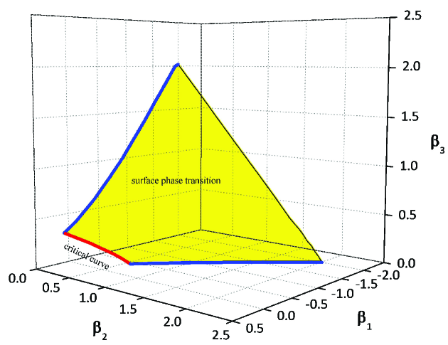
Figure 1. Phase transition surface $S$ and critical curve $C_{3}$. Graph drawn for $p=3$ and $q=5$.

By (4) and (5), the analyticity (or lack thereof) of the limiting free energy density $\psi_{\infty}^{\beta}$ encodes important information about the local features of the random graph $G_{n}$ for large $n$: A (jump) discontinuity in the first derivatives of $\psi_{\infty}^{\beta}$ across the surface $S$ indicates a discontinuity in the expected local densities, while the divergence of the second derivatives of $\psi_{\infty}^{\beta}$ along the curve $C_{3}$ implies that the covariances of the local densities go to zero more slowly than $1/n^{2}$.

Corollary 1.3.

The parameter space $\{(\beta_{1},\beta_{2},\beta_{3}):\beta_{2}\geq 0,\beta_{3}\geq 0\}$ consists of a single phase with a first order phase transition across the surface $S$ and a second order phase transition along the critical curve $C_{3}$.

Remark.

The requirement that the number of edges $p$ in $H_{2}$ and the number of edges $q$ in $H_{3}$ satisfy $2\leq p\leq q\leq 5p-1$ in the Assumptions is just a technicality. It is expected that the parameter space would still consist of a single phase with first order phase transition(s) across one (or more) surfaces and second order phase transition(s) along the critical curves should such assumptions fail.

To derive these results, we will make use of two theorems from [8], which connect the occurrence of a phase transition in our model with the solution of a certain maximization problem (a more extensive explanation may be found in [13]).

Theorem 1.4 (Theorem 4.1 in [8]).

Consider a general $k$-parameter exponential random graph model (1). Suppose $\beta_{2},...,\beta_{k}$ are non-negative. Then the limiting free energy density $\displaystyle\psi_{\infty}^{\beta}$ exists, and is given by

$$\psi_{\infty}^{\beta}=\sup_{0\leq u\leq 1}\left(\beta_{1}u^{E(H_{1})}+\cdots+\beta_{k}u^{E(H_{k})}-\frac{1}{2}u\log u-\frac{1}{2}(1-u)\log(1-u)\right)\\ ,$$ (8)

where $E(H_{i})$ is the number of edges in $H_{i}$.

Theorem 1.5 (Theorem 4.2 in [8]).

Let $G_{n}$ be an exponential random graph drawn from (1). Suppose $\beta_{2},...,\beta_{k}$ are non-negative. Then $G_{n}$ behaves like an Erdős-Rényi graph $G(n,u^{*})$ in the large n limit, where $u^{*}$ is picked randomly from the set $U$ of maximizers of (8).

Given the Chatterjee-Diaconis result, computing phase boundaries for the exponential model (6) mainly reduces to a $3$-dimensional calculus problem coupled with probability estimates. However, as straight-forward as it sounds, to get a clear picture of the limiting probability distribution and hence the global structure of a typical random graph $G_{n}$ drawn from this model, we need to solve the intricate calculus problem explicitly and employ various tricks. This mechanism may be generalized to a $k$-parameter setting (1), and the crucial idea (as will be illustrated in the proof of Proposition 2.1) is to minimize the effect of the ordered parameters on the limiting free energy density one by one.

The rest of this paper is organized as follows. In Section 2 we analyze the maximization problem (8) for $k=3$ in detail (Proposition 2.1) and describe the transition surface $S$ and the bounding curves $C_{1}$, $C_{2}$, and $C_{3}$ explicitly (Proposition 2.3). In Section 3 we investigate the analyticity properties of the limiting free energy density $\psi^{\beta}_{\infty}$ in different parameter regions (Theorems 3.1 and 3.3) and complete the proof of our main theorem (Theorem 1.2).

2. Maximization Analysis

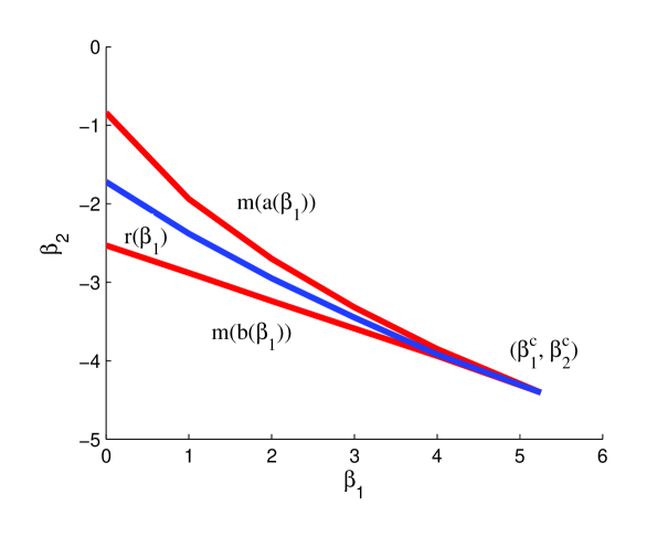
Figure 2. The V-shaped region (with phase transition curve $r(\beta_{1})$ inside) in the $(\beta_{1},\beta_{2})$ plane. Graph drawn for $\beta_{3}=2$, $p=3$, and $q=5$.

Proposition 2.1.

Fix $\beta_{3}$ and integers $p$ and $q$ with $2\leq p\leq q\leq 5p-1$. Consider the maximization problem for

$$l_{\beta_{3}}(u;\beta_{1},\beta_{2})=\beta_{1}u+\beta_{2}u^{p}+\beta_{3}u^{q}-\frac{1}{2}u\log u-\frac{1}{2}(1-u)\log(1-u)$$ (9)

on the interval $[0,1]$, where $-\infty<\beta_{1}<\infty$ and $-\infty<\beta_{2}<\infty$ are parameters. Then there is a V-shaped region in the $(\beta_{1},\beta_{2})$ plane with corner point $(\beta_{1}^{c},\beta_{2}^{c})$,

$$\beta_{1}^{c} = \frac{1}{2}\log\frac{u_{0}}{1-u_{0}}-\frac{1}{2(p-1)(1-u_{0})}+\frac{pu_{0}-(p-1)}{2(p-1)(q-1)(1-u_{0})^{2}},$$

$$\beta_{2}^{c} = \frac{qu_{0}-(q-1)}{2p(p-1)(p-q)u_{0}^{p-1}(1-u_{0})^{2}},$$ (10)

where $u_{0}$ is uniquely determined by

$$\beta_{3}=\frac{pu_{0}-(p-1)}{2q(q-1)(q-p)u_{0}^{q-1}(1-u_{0})^{2}}.$$ (11)

Outside this region, $l_{\beta_{3}}(u)$ has only one local maximizer (hence global maximizer) $u^{*}$; Inside this region, $l_{\beta_{3}}(u)$ has exactly two local maximizers $u_{1}^{*}$ and $u_{2}^{*}$. For every $\beta_{1}$ inside this V-shaped region ($\beta_{1}<\beta_{1}^{c}$), there is a unique decreasing $\beta_{2}=r_{\beta_{3}}(\beta_{1})$ such that $u_{1}^{*}$ and $u_{2}^{*}$ are both global maximizers for $l_{\beta_{3}}(u;\beta_{1},r_{\beta_{3}}(\beta_{1}))$ (see Figures 2 and 3).

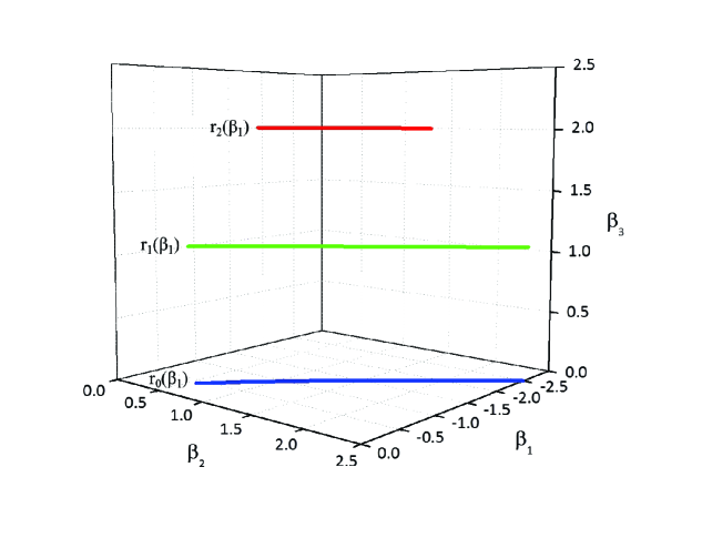
Figure 3. The phase transition curves $r(\beta_{1})$ (corresponding to $\beta_{3}=0$, $\beta_{3}=1$, and $\beta_{3}=2$) in the $(\beta_{1},\beta_{2},\beta_{3})$ space. Graph drawn for $p=3$ and $q=5$.

Proof.

The location of maximizers of $l_{\beta_{3}}(u)$ on the interval $[0,1]$ is closely related to the properties of its derivatives $l^{\prime}_{\beta_{3}}(u)$ and $l^{\prime\prime}_{\beta_{3}}(u)$:

$$l^{\prime}_{\beta_{3}}(u)=\beta_{1}+p\beta_{2}u^{p-1}+q\beta_{3}u^{q-1}-\frac{1}{2}\log\frac{u}{1-u},$$ (12)

$$l^{\prime\prime}_{\beta_{3}}(u)=p(p-1)\beta_{2}u^{p-2}+q(q-1)\beta_{3}u^{q-2}-\frac{1}{2u(1-u)}.$$ (13)

We first analyze the properties of $l^{\prime\prime}_{\beta_{3}}(u)$ on the interval $[0,1]$. Consider instead

$$F(u)=p(p-1)\beta_{2}+q(q-1)\beta_{3}u^{q-p}-\frac{1}{2u^{p-1}(1-u)},$$ (14)

which is obtained by factorizing $u^{p-2}$ out of $l^{\prime\prime}_{\beta_{3}}(u)$. Note that in doing so the effect of $\beta_{2}$ is minimized as varying $\beta_{2}$ only shifts the graph of $F(u)$ upward/downward and does not affect its shape. To examine the effect of $\beta_{3}$ on $F(u)$, we take one more derivative,

$$F^{\prime}(u)=q(q-1)(q-p)\beta_{3}u^{q-p-1}+\frac{(p-1)-pu}{2u^{p}(1-u)^{2}}.$$ (15)

Similarly as before, we factor $u^{q-p-1}$ out of $F^{\prime}(u)$ to minimize the effect of $\beta_{3}$. Let

$$f(u)=\frac{(p-1)-pu}{u^{q-1}(1-u)^{2}}$$ (16)

so that

$$F^{\prime}(u)=\frac{1}{2}u^{q-p-1}(2q(q-1)(q-p)\beta_{3}+f(u)).$$ (17)

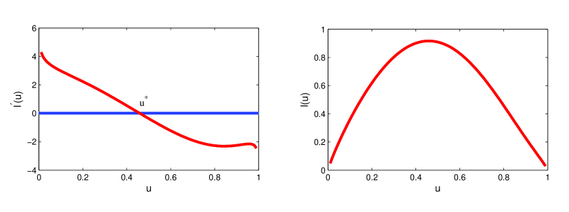
Figure 4. Outside the V-shaped region, $l_{\beta_{3}}(u)$ has a unique local maximizer (hence global maximizer) $u^{*}$. Graph drawn for $\beta_{1}=2$, $\beta_{2}=-4$, $\beta_{3}=2$, $p=3$, and $q=5$.

We claim that the condition $2\leq p\leq q\leq 5p-1$ guarantees that $f(u)$ is monotonically decreasing on $[0,1]$. Independent of $p$ and $q$, $f(0)=\infty$ and $f(1)=-\infty$. Its derivative $f^{\prime}(u)$ is given by

$$f^{\prime}(u)=-\frac{pqu^{2}+(p+q+1-2pq)u+(p-1)(q-1)}{u^{q}(1-u)^{3}}.$$ (18)

Rearranging terms in the discriminant $\Delta$ of the numerator of $f^{\prime}(u)$ yields a quadratic equation in $q$,

$$\Delta=q^{2}+2(1-3p)q+(p+1)^{2}$$ (19)

with two zeros

$$q_{1,2}=(3p-1)\pm 2\sqrt{2(p^{2}-p)}.$$ (20)

We can easily check that $q_{1}\leq p$ and $q_{2}\geq 5p-1$. As $q_{1}\leq q\leq q_{2}$ is equivalent to $\Delta\leq 0$, this verifies our claim.

An immediate corollary is that there is a unique $u_{0}$ in $(0,1)$ such that $F^{\prime}(u_{0})=0$, with $F^{\prime}(u)>0$ for $u<u_{0}$, and $F^{\prime}(u)<0$ for $u>u_{0}$. The correspondence between $\beta_{3}$ and $u_{0}$ is one-to-one, and we may alternatively describe $\beta_{3}$ by

$$\beta_{3}=\frac{pu_{0}-(p-1)}{2q(q-1)(q-p)u_{0}^{q-1}(1-u_{0})^{2}}.$$ (21)

This further implies that $F(u)$ is increasing from $0$ to $u_{0}$, and decreasing from $u_{0}$ to $1$, with the global maximum achieved at $u_{0}$,

$$F(u_{0})=p(p-1)\beta_{2}+\frac{qu_{0}-(q-1)}{2(q-p)u_{0}^{p-1}(1-u_{0})^{2}}.$$ (22)

Let

$$\beta_{2}^{c}=\frac{qu_{0}-(q-1)}{2p(p-1)(p-q)u_{0}^{p-1}(1-u_{0})^{2}}$$ (23)

so that $F(u_{0};\beta_{2}^{c})=0$. As $F(u)$ and $l^{\prime\prime}_{\beta_{3}}(u)$ always carry the same sign, this shows that for $\beta_{2}\leq\beta_{2}^{c}$, $l^{\prime\prime}_{\beta_{3}}(u)\leq 0$ on the whole interval $[0,1]$; whereas for $\beta_{2}>\beta_{2}^{c}$, $l^{\prime\prime}_{\beta_{3}}(u)$ takes on both positive and negative values, and we denote the transition points by $u_{1}$ and $u_{2}$ ($u_{1}<u_{0}<u_{2}$), which are solely determined by $\beta_{2}$, and vice versa. Let

$$m(u)=\frac{1}{2p(p-1)u^{p-1}(1-u)}+\frac{(p-1)-pu_{0}}{2p(p-1)(q-p)u_{0}^{q-1}(1-u_{0})^{2}}u^{q-p}$$ (24)

so that $\beta_{2}=m(u_{1})=m(u_{2})$. As $m(u)=\beta_{2}-F(u)/p(p-1)$, we have $m(0)=m(1)=\infty$, $m(u)$ is decreasing from $0$ to $u_{0}$, and increasing from $u_{0}$ to $1$.

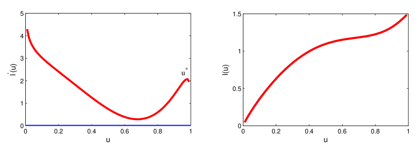
Figure 5. Outside the V-shaped region, $l_{\beta_{3}}(u)$ has a unique local maximizer (hence global maximizer) $u^{*}$. Graph drawn for $\beta_{1}=2$, $\beta_{2}=-2.5$, $\beta_{3}=2$, $p=3$, and $q=5$.

Based on the properties of $l^{\prime\prime}_{\beta_{3}}(u)$, we next analyze the properties of $l^{\prime}_{\beta_{3}}(u)$ on the interval $[0,1]$. For $\beta_{2}\leq\beta_{2}^{c}$, $l^{\prime}_{\beta_{3}}(u)$ is monotonically decreasing. For $\beta_{2}>\beta_{2}^{c}$, $l^{\prime}_{\beta_{3}}(u)$ is decreasing from $0$ to $u_{1}$, increasing from $u_{1}$ to $u_{2}$, then decreasing again from $u_{2}$ to $1$. For reasons that will become clear in a moment, we write down the explicit expressions of $l^{\prime}_{\beta_{3}}(u_{1})$ and $l^{\prime}_{\beta_{3}}(u_{2})$:

$$l^{\prime}_{\beta_{3}}(u_{1})=\beta_{1}+\frac{1}{2(p-1)(1-u_{1})}-\frac{1}{2}\log\frac{u_{1}}{1-u_{1}}+\frac{(p-1)-pu_{0}}{2(p-1)(q-1)u_{0}^{q-1}(1-u_{0})^{2}}u_{1}^{q-1},$$ (25)

$$l^{\prime}_{\beta_{3}}(u_{2})=\beta_{1}+\frac{1}{2(p-1)(1-u_{2})}-\frac{1}{2}\log\frac{u_{2}}{1-u_{2}}+\frac{(p-1)-pu_{0}}{2(p-1)(q-1)u_{0}^{q-1}(1-u_{0})^{2}}u_{2}^{q-1}.$$ (26)

Finally, based on the properties of $l^{\prime}_{\beta_{3}}(u)$ and $l^{\prime\prime}_{\beta_{3}}(u)$, we analyze the properties of $l_{\beta_{3}}(u)$ on the interval $[0,1]$. Independent of $p$ and $q$, $l_{\beta_{3}}(u)$ is a bounded continuous function, $l^{\prime}_{\beta_{3}}(0)=\infty$, and $l^{\prime}_{\beta_{3}}(1)=-\infty$, so $l_{\beta_{3}}(u)$ can not be maximized at $0$ or $1$. For $\beta_{2}\leq\beta_{2}^{c}$, $l^{\prime}_{\beta_{3}}(u)$ crosses the $u$-axis only once, going from positive to negative. Thus $l_{\beta_{3}}(u)$ has a unique local maximizer (hence global maximizer) $u^{*}$. For $\beta_{2}>\beta_{2}^{c}$, the situation is more complicated. If $l^{\prime}_{\beta_{3}}(u_{1})\geq 0$ (resp. $l^{\prime}_{\beta_{3}}(u_{2})\leq 0$), $l_{\beta_{3}}(u)$ has a unique local maximizer (hence global maximizer) at a point $u^{*}>u_{2}$ (resp. $u^{*}<u_{1}$). If $l^{\prime}_{\beta_{3}}(u_{1})<0<l^{\prime}_{\beta_{3}}(u_{2})$, then $l_{\beta_{3}}(u)$ has two local maximizers $u_{1}^{*}$ and $u_{2}^{*}$, with $u_{1}^{*}<u_{1}<u_{0}<u_{2}<u_{2}^{*}$ (see Figures 4 and 5).

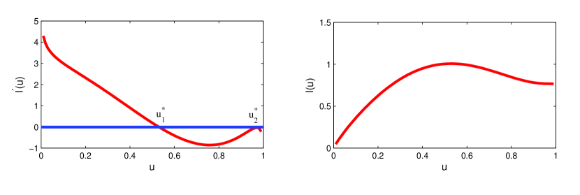
Figure 6. Along the lower bounding curve $m(b(\beta_{1}))$ of the V-shaped region, $l^{\prime}_{\beta_{3}}(u)$ has two zeros $u_{1}^{*}$ and $u_{2}^{*}$, but only $u_{1}^{*}$ is the global maximizer for $l_{\beta_{3}}(u)$. Graph drawn for $\beta_{1}=2$, $\beta_{2}=-3.24$, $\beta_{3}=2$, $p=3$, and $q=5$.

Let

$$n(u)=\frac{1}{2(p-1)(1-u)}-\frac{1}{2}\log\frac{u}{1-u}+\frac{(p-1)-pu_{0}}{2(p-1)(q-1)u_{0}^{q-1}(1-u_{0})^{2}}u^{q-1}$$ (27)

so that $l^{\prime}_{\beta_{3}}(u_{1})=\beta_{1}+n(u_{1})$ and $l^{\prime}_{\beta_{3}}(u_{2})=\beta_{1}+n(u_{2})$. Independent of $p$ and $q$, $n(0)=\infty$ and $n(1)=\infty$. Its derivative $n^{\prime}(u)$ is given by

$$n^{\prime}(u) = \frac{1}{2(p-1)}u^{q-2}\left(\frac{(p-1)-pu_{0}}{u_{0}^{q-1}(1-u_{0})^{2}}-\frac{(p-1)-pu}{u^{q-1}(1-u)^{2}}\right)$$ (28)

$$= \frac{1}{2(p-1)}u^{q-2}\left(f(u_{0})-f(u)\right).$$

As $f(u)$ is monotonically decreasing, $n(u)$ is decreasing from $0$ to $u_{0}$, and increasing from $u_{0}$ to $1$, with the global minimum achieved at $u_{0}$,

$$n(u_{0})=\frac{1}{2(p-1)(1-u_{0})}-\frac{1}{2}\log\frac{u_{0}}{1-u_{0}}+\frac{(p-1)-pu_{0}}{2(p-1)(q-1)(1-u_{0})^{2}}.$$ (29)

This implies that $l^{\prime}_{\beta_{3}}(u_{1};\beta_{1},\beta_{2}^{c})\geq 0$ for

$$\beta_{1}\geq\beta_{1}^{c}=\frac{1}{2}\log\frac{u_{0}}{1-u_{0}}-\frac{1}{2(p-1)(1-u_{0})}+\frac{pu_{0}-(p-1)}{2(p-1)(q-1)(1-u_{0})^{2}}.$$ (30)

The only possible region in the $(\beta_{1},\beta_{2})$ plane where $l^{\prime}_{\beta_{3}}(u_{1})<0<l^{\prime}_{\beta_{3}}(u_{2})$ is thus bounded by $\beta_{1}<\beta_{1}^{c}$ and $\beta_{2}>\beta_{2}^{c}$.

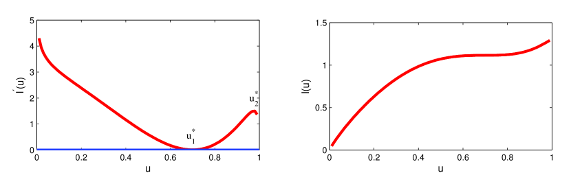
Figure 7. Along the upper bounding curve $m(a(\beta_{1}))$ of the V-shaped region, $l^{\prime}_{\beta_{3}}(u)$ has two zeros $u_{1}^{*}$ and $u_{2}^{*}$, but only $u_{2}^{*}$ is the global maximizer for $l_{\beta_{3}}(u)$. Graph drawn for $\beta_{1}=2$, $\beta_{2}=-2.7$, $\beta_{3}=2$, $p=3$, and $q=5$.

We now analyze the behavior of $l^{\prime}_{\beta_{3}}(u_{1})$ and $l^{\prime}_{\beta_{3}}(u_{2})$ more closely when $\beta_{1}$ and $\beta_{2}$ are chosen from this region. Recall that $u_{1}<u_{0}<u_{2}$. By monotonicity of $n(u)$ on the intervals $(0,u_{0})$ and $(u_{0},1)$, there exist continuous functions $a(\beta_{1})$ and $b(\beta_{1})$ of $\beta_{1}$, such that $l^{\prime}_{\beta_{3}}(u_{1})<0$ for $u_{1}>a(\beta_{1})$ and $l^{\prime}_{\beta_{3}}(u_{2})>0$ for $u_{2}>b(\beta_{1})$. As $\beta_{1}\to-\infty$, $a(\beta_{1})\to 0$ and $b(\beta_{1})\to 1$. $a(\beta_{1})$ is an increasing function of $\beta_{1}$, whereas $b(\beta_{1})$ is a decreasing function, and they satisfy

$$n(a(\beta_{1}))=n(b(\beta_{1}))=-\beta_{1}.$$ (31)

The restrictions on $u_{1}$ and $u_{2}$ yield restrictions on $\beta_{2}$, and we have $l^{\prime}_{\beta_{3}}(u_{1})<0$ for $\beta_{2}<m(a(\beta_{1}))$ and $l^{\prime}_{\beta_{3}}(u_{2})>0$ for $\beta_{2}>m(b(\beta_{1}))$. As $\beta_{1}\to-\infty$, $m(a(\beta_{1}))\to\infty$ and $m(b(\beta_{1}))\to\infty$. $m(a(\beta_{1}))$ and $m(b(\beta_{1}))$ are both decreasing functions of $\beta_{1}$, and they satisfy

$$l^{\prime}_{\beta_{3}}(u_{1};\beta_{1},m(a(\beta_{1})))=l^{\prime}_{\beta_{3}}(u_{2};\beta_{1},m(b(\beta_{1})))=0.$$ (32)

As $l^{\prime}_{\beta_{3}}(u_{2};\beta_{1},\beta_{2})>l^{\prime}_{\beta_{3}}(u_{1};\beta_{1},\beta_{2})$ for every $(\beta_{1},\beta_{2})$, the curve $m(b(\beta_{1}))$ must lie below the curve $m(a(\beta_{1}))$, and together they generate the bounding curves of the V-shaped region in the $(\beta_{1},\beta_{2})$ plane with corner point $(\beta_{1}^{c},\beta_{2}^{c})$ where two local maximizers exist for $l_{\beta_{3}}(u)$ (see Figures 6 and 7).

Fix an arbitrary $\beta_{1}<\beta_{1}^{c}$, we examine the effect of varying $\beta_{2}$ on the graph of $l^{\prime}_{\beta_{3}}(u)$. It is clear that $l^{\prime}_{\beta_{3}}(u)$ shifts upward as $\beta_{2}$ increases and downward as $\beta_{2}$ decreases. As a result, as $\beta_{2}$ gets large, the positive area bounded by the curve $l^{\prime}_{\beta_{3}}(u)$ increases, whereas the negative area decreases. By the fundamental theorem of calculus, the difference between the positive and negative areas is the difference between $l_{\beta_{3}}(u_{2}^{*})$ and $l_{\beta_{3}}(u_{1}^{*})$, which goes from negative ($l^{\prime}_{\beta_{3}}(u_{2})=0$, $u_{1}^{*}$ is the global maximizer) to positive ($l^{\prime}_{\beta_{3}}(u_{1})=0$, $u_{2}^{*}$ is the global maximizer) as $\beta_{2}$ goes from $m(b(\beta_{1}))$ to $m(a(\beta_{1}))$. Thus there must be a unique $\beta_{2}:m(b(\beta_{1}))<\beta_{2}<m(a(\beta_{1}))$ such that $u_{1}^{*}$ and $u_{2}^{*}$ are both global maximizers, and we denote this $\beta_{2}$ by $r_{\beta_{3}}(\beta_{1})$ (see Figure 8). The parameter values of $(\beta_{1},r_{\beta_{3}}(\beta_{1}))$ are exactly the ones for which positive and negative areas bounded by $l^{\prime}_{\beta_{3}}(u)$ equal each other. An increase in $\beta_{1}$ induces an upward shift of $l^{\prime}_{\beta_{3}}(u)$, and must be balanced by a decrease in $\beta_{2}$. Similarly, a decrease in $\beta_{1}$ induces a downward shift of $l^{\prime}_{\beta_{3}}(u)$, and must be balanced by an increase in $\beta_{2}$. This justifies that $r_{\beta_{3}}$ is monotonically decreasing in $\beta_{1}$. ∎

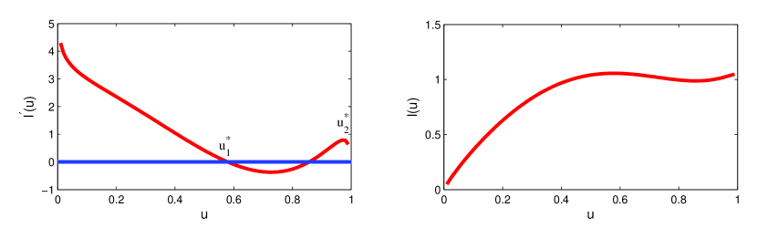
Figure 8. Along the phase transition curve $r(\beta_{1})$, $l_{\beta_{3}}(u)$ has two local maximizers $u_{1}^{*}$ and $u_{2}^{*}$, and both are global maximizers for $l_{\beta_{3}}(u)$. Graph drawn for $\beta_{1}=2$, $\beta_{2}=-2.95$, $\beta_{3}=2$, $p=3$, and $q=5$.

The following universality result shows that independent of the specific local features that are incorporated into the exponential random graph model (6), the transition surface $S$ asymptotically approaches a common plane $\beta_{1}+\beta_{2}+\beta_{3}=0$.

Corollary 2.2 (Universality).

Fix $\beta_{3}\geq 0$. The transition curve $\beta_{2}=r_{\beta_{3}}(\beta_{1})$ displays a universal asymptotic behavior as $\beta_{1}\to-\infty$:

$$\lim_{\beta_{1}\to-\infty}|r_{\beta_{3}}(\beta_{1})+\beta_{1}+\beta_{3}|=0.$$ (33)

Proof.

By Proposition 2.1, it suffices to show that as $\beta_{1}\to-\infty$, $l_{\beta_{3}}(u;\beta_{1},-\beta_{1}-\beta_{3})$ has two global maximizers $u_{1}^{*}$ and $u_{2}^{*}$. This is easy when we realize that as $\beta_{1}\to-\infty$, $l_{\beta_{3}}(u;\beta_{1},-\beta_{1}-\beta_{3})\to-\infty$ for every $u$ in $(0,1)$. The limiting maximizers on $[0,1]$ are thus $u_{1}^{*}=0$ and $u_{2}^{*}=1$, with $l_{\beta_{3}}(u_{1}^{*})=l_{\beta_{3}}(u_{2}^{*})=0$. ∎

Proposition 2.3.

As $\beta_{3}\geq 0$ varies, the transition curves $\beta_{2}=r_{\beta_{3}}(\beta_{1})$ (subject to $\beta_{2}\geq 0$) trace out a continuous surface $S$ with three bounding curves $C_{1}$, $C_{2}$, and $C_{3}$.

Proof.

The continuity of the transition surface $S$ follows easily once we realize that it consists exactly of parameter values of $(\beta_{1},\beta_{2},\beta_{3})$ for which $l_{\beta_{3}}(u)$ (continuous in $\beta_{1}$, $\beta_{2}$, and $\beta_{3}$) has two global maximizers. By Corollary 2.2, $S$ displays a universal asymptotic behavior: As $\beta_{1}\to-\infty$, $\beta_{2}\to\infty$, and $\beta_{3}\to\infty$, the distance between $S$ and the plane $\beta_{1}+\beta_{2}+\beta_{3}=0$ shrinks to zero. Due to the non-negativity constraints on $\beta_{2}$ and $\beta_{3}$, $S$ is bounded by three curves $C_{1}$, $C_{2}$, and $C_{3}$: The curve $C_{1}$ is the intersection of $S$ with the ($\beta_{1}$, $\beta_{2}$) plane, and is given by $\beta_{2}=r_{0}(\beta_{1})$ (cf. Proposition 2.1); The curve $C_{2}$ is the intersection of $S$ with the ($\beta_{1}$, $\beta_{3}$) plane, and is given analogously (with $p$ and $q$ switched in (9)); The curve $C_{3}$ is a critical curve, and is traced out by the critical points $(\beta_{1}^{c},\beta_{2}^{c})$ (2.1) (subject to $\beta_{2}^{c}\geq 0$). ∎

3. Critical Behavior

By Propositions 2.1 and 2.3, the maximization problem (9) is solved at a unique value $u^{*}$ off $S$, and at two values $u_{1}^{*}$ and $u_{2}^{*}$ on $S$ (the jump from $u_{1}^{*}$ to $u_{2}^{*}$ is quite noticeable even for small parameter values of $\beta$). Thus by Theorems 1.4 and 1.5, in the large $n$ limit, a typical $G_{n}$ drawn from (1) is indistinguishable from the Erdős-Rényi graph $G(n,u^{*})$ off the transition surface $S$, however, on the transition surface $S$, the structure of $G_{n}$ is not completely deterministic: It may behave like an Erdős-Rényi graph $G(n,u_{1}^{*})$, or it may behave like an Erdős-Rényi graph $G(n,u_{2}^{*})$. Since the limiting free energy density $\psi_{\infty}^{\beta}$ encodes important information about the local features of the random graph $G_{n}$ (see for example (4) and (5)), a thorough study of its analyticity properties is fundamental to understanding the global structure of the exponential model. The following theorems 3.1 and 3.3 are dedicated to this goal. Together they complete the proof of our main theorem (Theorem 1.2).

Theorem 3.1.

Consider a $3$-parameter exponential random graph model (6). The limiting free energy density $\displaystyle\psi_{\infty}^{\beta}$ is not an analytic function on the transition surface $S$.

Proof.

Due to the jump between the two solutions $u_{1}^{*}$ and $u_{2}^{*}$ of the maximization problem (9), all the first derivatives $\displaystyle\frac{\partial}{\partial\beta_{1}}\psi_{\infty}^{\beta}$, $\displaystyle\frac{\partial}{\partial\beta_{2}}\psi_{\infty}^{\beta}$, and $\displaystyle\frac{\partial}{\partial\beta_{3}}\psi_{\infty}^{\beta}$ have (jump) discontinuities across the transition surface $S$, except along the critical curve $C_{3}$:

$$\lim_{n\to\infty}\mathbb{E}^{\beta}t(H_{1},G_{n})=\lim_{n\to\infty}\mathbb{E}^{\beta}t(H_{1},G(n,u^{*}))=u^{*}=\frac{\partial}{\partial\beta_{1}}\psi_{\infty}^{\beta},$$ (34)

$$\lim_{n\to\infty}\mathbb{E}^{\beta}t(H_{2},G_{n})=\lim_{n\to\infty}\mathbb{E}^{\beta}t(H_{2},G(n,u^{*}))=(u^{*})^{p}=\frac{\partial}{\partial\beta_{2}}\psi_{\infty}^{\beta},$$ (35)

$$\lim_{n\to\infty}\mathbb{E}^{\beta}t(H_{3},G_{n})=\lim_{n\to\infty}\mathbb{E}^{\beta}t(H_{3},G(n,u^{*}))=(u^{*})^{q}=\frac{\partial}{\partial\beta_{3}}\psi_{\infty}^{\beta}.$$ (36)

To see that the transition across $C_{3}$ is second-order, we check the first and second derivatives of $\psi_{\infty}^{\beta}$ in the neighborhood of this curve. By Proposition 2.1, for every $(\beta_{1}^{c},\beta_{2}^{c},\beta_{3})$ on $C_{3}$, $l^{\prime}_{\beta_{3}}(u;\beta_{1}^{c},\beta_{2}^{c})$ is monotonically decreasing on $[0,1]$, and the unique zero is achieved at $u_{0}$ (11). Take any $0<\epsilon<\min\{u_{0},1-u_{0}\}$. Set $\displaystyle\delta=\min\{l^{\prime}_{\beta_{3}}(u_{0}-\epsilon),-l^{\prime}_{\beta_{3}}(u_{0}+\epsilon)\}$. Consider $(\bar{\beta}_{1},\bar{\beta}_{2},\bar{\beta}_{3})$ so close to $(\beta_{1}^{c},\beta_{2}^{c},\beta_{3})$ such that $\displaystyle|\bar{\beta}_{1}-\beta_{1}^{c}|+p|\bar{\beta}_{2}-\beta_{2}^{c}|+q|\bar{\beta}_{3}-\beta_{3}|<\delta$. For every $u$ in $[0,1]$, we then have $\displaystyle\left|l^{\prime}_{\bar{\beta}_{3}}(u;\bar{\beta}_{1},\bar{\beta}_{2})-l^{\prime}_{\beta_{3}}(u;\beta_{1}^{c},\beta_{2}^{c})\right|<\delta$. It follows that the zero $u^{*}(\bar{\beta}_{1},\bar{\beta}_{2},\bar{\beta}_{3})$ (or $u_{1}^{*}$ and $u_{2}^{*}$) must satisfy $\left|u^{*}-u_{0}\right|<\epsilon$, which easily implies the continuity of $\displaystyle\frac{\partial}{\partial\beta_{1}}\psi_{\infty}^{\beta}$, $\displaystyle\frac{\partial}{\partial\beta_{2}}\psi_{\infty}^{\beta}$, and $\displaystyle\frac{\partial}{\partial\beta_{3}}\psi_{\infty}^{\beta}$ at $(\beta_{1}^{c},\beta_{2}^{c},\beta_{3})$. Concerning the divergence of the second derivatives, we compute

$$\frac{\partial^{2}}{\partial\beta_{1}^{2}}\psi_{\infty}^{\beta}=\frac{\partial}{\partial\beta_{1}}u^{*}=-\frac{1}{l^{\prime\prime}_{\beta_{3}}(u^{*})},\hskip 28.45274pt\frac{\partial^{2}}{\partial\beta_{2}^{2}}\psi_{\infty}^{\beta}=\frac{\partial}{\partial\beta_{2}}(u^{*})^{p}=-\frac{p^{2}(u^{*})^{2p-2}}{l^{\prime\prime}_{\beta_{3}}(u^{*})},$$ (37)

$$\frac{\partial^{2}}{\partial\beta_{3}^{2}}\psi_{\infty}^{\beta}=\frac{\partial}{\partial\beta_{3}}(u^{*})^{q}=-\frac{q^{2}(u^{*})^{2q-2}}{l^{\prime\prime}_{\beta_{3}}(u^{*})},\hskip 28.45274pt\frac{\partial^{2}}{\partial\beta_{1}\partial\beta_{2}}\psi_{\infty}^{\beta}=\frac{\partial}{\partial\beta_{1}}(u^{*})^{p}=-\frac{p(u^{*})^{p-1}}{l^{\prime\prime}_{\beta_{3}}(u^{*})},$$ (38)

$$\frac{\partial^{2}}{\partial\beta_{1}\partial\beta_{3}}\psi_{\infty}^{\beta}=\frac{\partial}{\partial\beta_{1}}(u^{*})^{q}=-\frac{q(u^{*})^{q-1}}{l^{\prime\prime}_{\beta_{3}}(u^{*})},\hskip 28.45274pt\frac{\partial^{2}}{\partial\beta_{2}\partial\beta_{3}}\psi_{\infty}^{\beta}=\frac{\partial}{\partial\beta_{2}}(u^{*})^{q}=-\frac{pq(u^{*})^{p+q-2}}{l^{\prime\prime}_{\beta_{3}}(u^{*})}.$$ (39)

But as was explained in Proposition 2.1, as $(\bar{\beta}_{1},\bar{\beta}_{2},\bar{\beta}_{3})$ approaches $C_{3}$, $l^{\prime\prime}_{\bar{\beta}_{3}}(u^{*};\bar{\beta}_{1},\bar{\beta}_{2})$ converges to zero. The desired singularity is thus justified. ∎

Real and complex analyticity are both defined in terms of convergent power series. To examine the analyticity of the limiting free energy density $\psi_{\infty}^{\beta}$ off the transition surface $S$, we resort to an analytic implicit function theorem, which may be interpreted in either the real or the complex setting.

Theorem 3.2 (Krantz-Parks [19]).

Suppose that the power series

$$F(x,y)=\sum_{\alpha,k}a_{\alpha,k}{x}^{\alpha}y^{k}$$ (40)

is absolutely convergent for $|x|\leq R_{1}$ and $|y|\leq R_{2}$. If $a_{0,0}=0$ and $a_{0,1}\neq 0$, then there exist $r_{0}>0$ and a power series

$$f(x)=\sum_{|\alpha|>0}c_{\alpha}{x}^{\alpha}$$ (41)

such that (41) is absolutely convergent for $|x|\leq r_{0}$ and $F(x,f(x))=0$.

Theorem 3.3.

Consider a $3$-parameter exponential random graph model (6). Suppose $\beta_{2}$ and $\beta_{3}$ are non-negative. Then the limiting free energy density $\displaystyle\psi_{\infty}^{\beta}$ is an analytic function off the transition surface $S$.

Proof.

It is clear that $l_{\beta_{3}}(u;\beta_{1},\beta_{2})$ is analytic for $u\in(0,1)$, $\beta_{1}\in(-\infty,\infty)$, $\beta_{2}\in(-\infty,\infty)$, and $\beta_{3}\in(-\infty,\infty)$. We show that the maximizer $u^{*}$ for $l_{\beta_{3}}(u;\beta_{1},\beta_{2})$ is an analytic function of $\beta$ off the transition surface $S$. Fix $(\beta_{1},\beta_{2},\beta_{3})$ not on $S$. For $(\bar{\beta}_{1},\bar{\beta}_{2},\bar{\beta}_{3})$ close to $(\beta_{1},\beta_{2},\beta_{3})$, we transform the function $l^{\prime}_{\bar{\beta}_{3}}(u;\bar{\beta}_{1},\bar{\beta}_{2})$ into a function $F(x,y)$ by setting $x=(\bar{\beta}_{1}-\beta_{1},\bar{\beta}_{2}-\beta_{2},\bar{\beta}_{3}-\beta_{3})$ and $y=u-u^{*}(\beta_{1},\beta_{2},\beta_{3})$. It is easy to check that $F(x,y)$ satisfies all the conditions of Theorem 3.2: It has the desired domain of analyticity, is locally absolutely convergent, and its first two coefficients are given by

$$a_{0,0}=F(0,0)=l^{\prime}_{\beta_{3}}(u^{*}(\beta_{1},\beta_{2},\beta_{3});\beta_{1},\beta_{2})=0,$$ (42)

$$a_{0,1}=\frac{\partial F}{\partial y}(0,0)=l^{\prime\prime}_{\beta_{3}}(u^{*}(\beta_{1},\beta_{2},\beta_{3});\beta_{1},\beta_{2})\neq 0.$$ (43)

The absolute convergence for $f(x)=u^{*}(\bar{\beta}_{1},\bar{\beta}_{2},\bar{\beta}_{3})-u^{*}(\beta_{1},\beta_{2},\beta_{3})$ then follows easily, which implies the analyticity of $u^{*}$ as a function of $\beta$. As the composition of analytic functions is analytic as long as the domain and range match up, by Theorem 1.4, this further implies the analyticity of $\psi_{\infty}^{\beta}=l_{\beta_{3}}(u^{*};\beta_{1},\beta_{2})$ as a function of $\beta$ off the transition surface $S$, where the maximizer $u^{*}$ is uniquely defined. ∎

References

- [1] Besag, J.: Statistical analysis of non-lattice data. J. Roy. Statist. Soc. Ser. D 24, 179-195 (1975)
-
[2]
Hammersley, J., Clifford, P.: Markov fields on finite graphs and
lattices.
http://www.statslab.cam.ac.uk/grg/books/hammfest/hamm-cliff.pdf (1971) - [3] Holland, P., Leinhardt, S.: An exponential family of probability distributions for directed graphs. J. Amer. Statist. Assoc. 76, 33-50 (1981)
- [4] Frank, O., Strauss, D.: Markov graphs. J. Amer. Statist. Assoc. 81, 832-842 (1986)
- [5] Snijders, T., Pattison, P., Robins, G., Handcock M.: New specifications for exponential random graph models. Sociol. Method. 36, 99-153 (2006)
- [6] Rinaldo, A., Fienberg, S., Zhou, Y.: On the geometry of discrete exponential families with application to exponential random graph models. Electron. J. Stat. 3, 446-484 (2009)
- [7] Wasserman, S., Faust, K.: Social Network Analysis: Methods and Applications. Cambridge University Press, Cambridge (2010)
- [8] Chatterjee, S., Diaconis, P.: Estimating and understanding exponential random graph models. arXiv: 1102.2650v3 (2011)
- [9] Yang, C.N., Lee, T.D.: Statistical theory of equations of state and phase transitions. Phys. Rev. 87, 404-419 (1952)
- [10] Erdős, P., Rényi, A.: On the evolution of random graphs. Publ. Math. Inst. Hung. Acad. Sci. 5, 17-61 (1960)
- [11] Park, J., Newman, M.: Solution of the two-star model of a network. Phys. Rev. E 70, 066146 (2004)
- [12] Park, J., Newman, M.: Solution for the properties of a clustered network. Phys. Rev. E 72, 026136 (2005)
- [13] Lovász, L., Szegedy B.: Limits of dense graph sequences. J. Combin. Theory Ser. B 98, 933-957 (2006)
- [14] Häggström, O., Jonasson, J.: Phase transition in the random triangle model. J. Appl. Probab. 36, 1101-1115 (1999)
- [15] Bhamidi, S., Bresler, G., Sly, A.: Mixing time of exponential random graphs. Ann. Appl. Probab. 21, 2146-2170 (2011)
- [16] Radin, C., Yin, M.: Phase transitions in exponential random graphs. arXiv: 1108.0649v2 (2011)
- [17] Aristoff, D., Radin, C.: Emergent structures in large networks. arXiv: 1110.1912v1 (2011)
-
[18]
Yin, M.: Understanding exponential random graph
models.
http://www.ma.utexas.edu/users/myin/Talk.pdf (2012) - [19] Krantz, S., Parks, H.: The Implicit Function Theorem: History, Theory, and Applications. Birkhäuser, Boston (2002)