Analytical approximations to the core radius and energy of magnetic vortex in thin ferromagnetic disks

Abstract

The energy of magnetic vortex core and its equilibrium radius in thin circular cylinder were first presented by Usov and Peschany in 1994. Yet, the magnetostatic function, entering the energy expression, is hard to evaluate and approximate. Here, precise and explicit analytical approximations to this function (as well as equilibrium vortex core radius and energy) are derived in terms of elementary functions. Also, several simplifying approximations to the magnetic Hamiltonian and their impact on theoretical stability of magnetic vortex state are discussed.

1 Introduction

The first topological soliton was discovered as a solution of non-linear field theory equations by Skyrme[1]. It had a form of three-dimensional hedgehog and was named subsequently “skyrmion” in honor of the discoverer. After the landmark work of Belavin and Polyakov[2], topological solitons have crossed the boundary into condensed matter physics. The latter authors discovered much more topological soliton solutions in the infinite Heisenberg ferromagnet, as many as there are rational functions of complex variable, mapping any such function into some equilibrium magnetic structure. Zeros of numerator (possibly with higher multiplicity) of these rational functions correspond to the centers of magnetic vortices, while zeros of denominator to the centers of magnetic anti-vortices. In the model of infinite 2D ferromagnet, considered by Belavin and Polyakov, solitons are absolutely stable. Once magnetic texture with a certain topological charge (number of magnetic vortices) is created, all the structures with different topological charge are separated by an infinite energy barrier. It is worth noting that 7 years earlier essentially the same mathematics of rational functions of complex variable was applied to the problem of magnetic singularities (Bloch points) in 3D ferromagnet by Döring[3], who also found that the exchange energy of ferromagnet around a Bloch point depends only on degrees of numerator and denominator of the corresponding rational function. His energy expression is exactly the same as that of Belavin and Polyakov[2] for 2D ferromagnet. However (probably, because Bloch points, to which model of Ref. [3] applies, are rather exotic objects in magnetism), the paper by Döring is currently much less known and cited.

The model of Belavin and Polyakov became known in particle physics as non-linear O(3) $\sigma$ model in 3+1 dimensions and reformulated elegantly in terms of functions of complex variable by G. Woo[4]. David J. Gross found additional family of “meron” solutions to it[5]. Since then, the original Belavin-Polyakov solutions became known as just “solitons”. Merons, and all other O(3) $\sigma$ model solutions besides solitons[4], have infinite energy in unbounded 2-d ferromagnet, but can be realized when the ferromagnet is finite[6].

While these solutions were obtained long ago, the question of their stability has a history of its own. Kosterlitz and Thouless[7] analyzed stability of planar vortices in 2D ferromagnet and came to conclusion that they are unstable and such order could not exist. It is, indeed, true that the energy of Belavin-Polyakov solitons is scale-invariant and their size is, thus, undefined. In real ferromagnets, however, there are various other interactions (not exotic at all), which make the vortices stable. Usov and Peschany, were first to show that dipolar magnetostatic interaction stabilizes magnetic vortex in ferromagnetic cylinder both with respect to core radius change[8] and vortex center displacement[9]. Their results were later fully confirmed experimentally, starting with the direct observation of magnetic vortex core and measurement of its radius[10]. These and following experiments made single vortex state not only interesting from fundamental point of view, but also an essential component of emerging spintronic devices (such as MRAM elements, based on vortex core polarity[11] or chirality[12] switching, or spin-polarized current magnetic nano-oscillators[13]). It is also prerequisite for study of more complex multi-vortex magnetic configurations in planar nano-elements of various shapes.

Here, starting from recent (and more general) description of magnetization distributions in finite nano-elements via functions of complex variable [14] the impact of various approximations on vortex stability is reviewed in unified manner and the expression for vortex core radius in circular cylinder[8] is re-derived. It defines the core radius implicitly via an equation and an integral of certain special functions, which is very inconvenient to evaluate and approximate at small cylinder thickness because in this limit it is not analytic and its higher derivatives do not exist. It is, however, possible to introduce small parameters and expand the special functions and the vortex core radius into series, obtaining an explicit analytical approximate (but very precise) expressions, presented at the end.

2 Magnetic vortex in complex variables and its exchange energy

In finite planar nano-elements the equilibrium magnetization configurations can be described via rational functions of complex variable with real coefficients[14] (as opposed to complex coefficients in the case of infinite film[2, 4]). The simplest ansatz for magnetic vortex in circular cylinder (of thickness $L_{Z}$ and radius $R$) can be written in the complex notation as

$$f(z)=\imath(z-a)/R_{V}$$ (1)

where $z=X+\imath Y$ with $X$ and $Y$ being the Cartesian coordinates in the cylinder’s plane (the magnetization distribution is assumed to be independent on out-of-plane coordinate $Z$), $R_{V}$ is the vortex core radius and $a$ is the displacement of the vortex from the origin ($a=0$ corresponds to the centered vortex). Let us then define a complex function

$$w(z,\overline{z})=\left\{\begin{array}[]{ll}f(z)&|f(z)|\leq 1\\ f(z)/|f(z)|&|f(z)|>1\end{array}\right.,$$ (2)

where the line over variable denotes complex conjugation. The function $w$ is shown to depend explicitly on both $z$ and $\overline{z}$ because it is, in general, not holomorphic. It consists of two parts: soliton (where it is analytic and $\partial w(z,\overline{z})/\partial\overline{z}=0$) and meron (where $w\overline{w}=1$, joined at a line (possibly multiply-connected if there are several vortices or anti-vortices) $|f|=1$. The magnetization components, normalized by material’s saturation magnetization $M_{S}$, are then expressed via stereographic projection as

$$m_{x}+\imath m_{y} = \frac{2w(z,\overline{z})}{1+w(z,\overline{z})\overline{w}(z,\overline{z})}$$ (3)

$$m_{z} = \frac{1-w(z,\overline{z})\overline{w}(z,\overline{z})}{1+w(z,\overline{z})\overline{w}(z,\overline{z})}.$$ (4)

Being written via the magnetization components in Eq. (3)-(4), the ansatz in Eq.(1) is exactly equivalent to the one by Usov and Peschany[8] and also belongs to the class of trial functions, considered by Kosterlitz and Thouless[7]. Following the latter work, let us first take into account only the exchange interaction. In complex notation the exchange energy density (omitting the factor $C/2$, where $C$ is the exchange stiffness) can be directly expressed via the function $w$:

$$\sum_{i=x,y,z}(\vec{\nabla}m_{i})^{2}=\frac{8}{(1+w\overline{w})^{2}}\left(\frac{\partial w}{\partial z}\frac{\partial\overline{w}}{\partial\overline{z}}+\frac{\partial w}{\partial\overline{z}}\frac{\partial\overline{w}}{\partial z}\right),$$ (5)

where $\partial/\partial z=(\partial/\partial X-\imath\,\partial/\partial Y)/2$ and $\partial/\partial\overline{z}=(\partial/\partial X+\imath\,\partial/\partial Y)/2$. The total exchange energy can be obtained by integrating the density (5) over nano-element’s volume. Recalling the Riemann-Greene theorem

$$\frac{1}{2\imath}\oint_{\partial\cal D}u(\zeta,\overline{\zeta})\,{\mathrm{d}}\zeta=\iint_{\cal D}\frac{\partial u(z,\overline{z})}{\partial\overline{z}}\,{\mathrm{d}}X\,{\mathrm{d}}Y,$$ (6)

where $u$ is a complex function of the complex argument (not necessary analytic), it is possible to reduce the area integral over cylinder’s face $\cal D$ for the total exchange energy to a contour integral over its boundary $\partial\cal D$, provided there is a complex function, whose derivative over $\overline{z}$ yields the exchange energy density (5). Luckily, such function (actually two functions, one for soliton and one for meron part of $w$) can be easily obtained by direct integration of (5) with $w$ from each of the conditions in (2):

$$u^{S}(z,\overline{z}) = -\frac{8}{1+f(z)\overline{f}(\overline{z})}\frac{1}{f(z)}\frac{\partial f}{\partial z},$$ (7)

$$u^{\mathrm{M}}(z,\overline{z}) = \frac{1}{f(z)}\frac{\partial f}{\partial z}\log\left(f(z)\overline{f}(\overline{z})\right).$$ (8)

Thus, from (6), the total exchange energy inside the soliton is

$$\frac{E_{\mathrm{EX}}^{\mathrm{S}}}{CL_{Z}/2}=\frac{2}{\imath}\oint_{|f(\zeta)|=1}\frac{1}{f(\zeta)}\frac{\partial f(\zeta)}{\partial\zeta}\,{\mathrm{d}}\zeta,$$ (9)

where the fact that $|f(\zeta)|=1$ on the integration contour is used and the additional minus sign appears because the original contour of integration has to be walked clockwise. The function under the integral is analytic everywhere except the vortex centers $z_{i}$, where $f(z_{i})=0$. Assuming that line $|f(\zeta)|=1$ does not cross the particle boundary, it is possible to tighten the contours around each topological singularity (vortex or anti-vortex center) and use the residue theorem

$$\frac{E_{\mathrm{EX}}^{\mathrm{S}}}{CL_{Z}/2}=4\pi\sum_{i}\operatorname{Res}\left.\frac{1}{f(z)}\frac{\partial f(z)}{\partial z}\right|_{z\rightarrow z_{i}}.$$ (10)

In particular, for $f(z)$ from Eq. 1 this gives $E^{\mathrm{S}}/(CL_{Z}/2)=4\pi$. If there are several vortices inside the particle, the energy will be multiplied by their total number, including multiplicities.

For the meron part, the integration boundary is multiply-connected. However, on the inner boundaries (encircling solitons) $|f(\zeta)|=1$ and $u^{\mathrm{M}}(z,\overline{z})\sim\log 1=0$. Thus, only the integral over the cylinder’s outer boundary remains

$$\frac{E_{\mathrm{EX}}^{\mathrm{M}}}{CL_{Z}/2}=\frac{1}{2\imath}\oint_{\partial\cal D}\frac{1}{f(\zeta)}\frac{\partial f(\zeta)}{\partial\zeta}\log f(\zeta)\overline{f}(\overline{\zeta})\,{\mathrm{d}}\zeta$$ (11)

for $f(z)$ from Eq. 1 and the nano-element, shaped as circular cylinder ($\partial\cal D$ is $|z|=R$)

$$\frac{E_{\mathrm{EX}}^{\mathrm{M}}}{CL_{Z}/2} = \!\!\!\int\limits_{0}^{2\pi}\frac{(1\!-\!a\cos(\varphi)/R)\log\!\left(\frac{a^{2}-2aR\cos(\varphi)+R^{2}}{R_{V}^{2}}\right)}{2\left(a^{2}/R^{2}-2a\cos(\varphi)/R+1\right)}\,{\mathrm{d}}\varphi$$ (12)

$$= \pi\log\left(1-\frac{a^{2}}{R^{2}}\right)-2\pi\log\left(\frac{R_{V}}{R}\right),$$

and the total exchange energy $e_{\mathrm{EX}}=(E^{\mathrm{S}}+E^{\mathrm{M}})/(\mu_{0}\gamma_{B}M_{S}^{2}\pi R^{2}L_{Z})$ (in subsequent text all the dimensionless energies, denoted by small letter $e$ with different sub-/superscripts use the same normalization) is

$$e_{\mathrm{EX}}=\frac{L_{E}^{2}}{R^{2}}\left(2-\log\frac{R_{V}}{R}+\log\sqrt{1-\frac{a^{2}}{R^{2}}}\right),$$ (13)

where $\gamma_{B}=4\pi$, $\mu_{0}=1$ in CGS units and $\gamma_{B}=1$ in SI[15] and the exchange length $L_{E}=\sqrt{C/(\mu_{0}\gamma_{B}M_{S}^{2})}$. It can be seen immediately that the exchange energy decreases with increasing of the vortex core size $R_{V}$. The expression (13) is, formally, valid only for $R_{V}<R$, but it can be easily shown that the energy continues to decrease for larger $R_{V}$, reaching equilibrium for $R_{V}\rightarrow\infty$. This confirms the conclusion of Kosterlitz and Thouless[7] that magnetic vortices are unstable when only the exchange interaction is taken into account.

3 Magnetostatic energy of magnetic vortex

The long-range dipolar interaction between the local magnetic moments is present in all magnets. Strictly speaking, it is not instantaneous and its speed is limited by the speed of light. The account for retardation effects, however, contributes to the dissipation[16]. It is convenient (if magnetic nano-elements are small enough and characteristic timescales are large enough) to consider the dipolar interaction in magnetostatic approximation, making it non-local. Non-locality still poses a major mathematical difficulty, since it makes the equations for equilibrium magnetization distribution not only non-linear partial differential, but also integral. To alleviate this difficulty a number of local magnetostatic approximations had been developed. The most common (and very useful for considering domain walls in thin films) is based on using the local uniaxial in-plane anisotropy term $K_{\mathrm{MS}}m_{Z}^{2}$ instead of magnetostatic interaction. Selecting the local bulk anisotropy $K_{\mathrm{MS}}=\mu_{0}\gamma_{B}M_{S}^{2}/2$, one gets the exact correspondence between the approximate and exact magnetostatic energy density in two limiting cases: when the film is magnetized in-plane (magnetostatic energy is $0$) and out-of-plane (in which case the energy is $\mu_{0}\gamma_{B}M_{S}^{2}/2$). Nano-elements have additional side surfaces and it was recently proposed by Kohn and Slastikov[17] to use a similar expression for local surface anisotropy of magnetostatic origin on all surfaces with some a priori unknown constant $K_{s}$, replacing the $m_{Z}$ by a normal magnetization component on the surface. Let us try this approach.

3.1 Local anisotropy approximation

When vortex is completely inside the particle and is centered ($a=0$) the meron does not contribute to the anisotropy energy, and the contribution of soliton part is

$$e_{\mathrm{A}}^{in}=\frac{1}{R^{2}}\int\limits_{0}^{R_{V}}\frac{\left(r^{2}-R_{V}^{2}\right)^{2}}{\left(r^{2}+R_{V}^{2}\right)^{2}}r\,{\mathrm{d}}r=\frac{R_{V}^{2}}{R^{2}}\frac{\left(3-4\log 2\right)}{2}.$$ (14)

The total energy density $e_{\mathrm{EX}}+e_{\mathrm{A}}^{in}$ at $a=0$ now has a minimum when $R_{V}^{A}=L_{E}/\sqrt{3-4\log 2}$. Or, approximately, $R_{V}^{A}\approx 2.09698L_{E}=0.59155\sqrt{4\pi}L_{E}$, independent on cylinder’s thickness $L_{Z}$. The thickness independence is the result of expressing the magnetostatic energy in the form of surface anisotropy, and, as will be seen later, is wrong. Nevertheless, unlike the purely exchange approximation, the vortex core size is now stable. It is also worth noting that local anisotropy approximation is exact in the limit of vanishing film thickness, so that $R_{V}^{A}/L_{E}=\lim_{\lambda\rightarrow 0}\rho_{V}(\lambda)$, where $\rho_{V}(\lambda)$ is the vortex core radius, computed with full treatment of magnetostatics (23).

But stable vortex core size is not all, the vortex must also be stable with respect to the displacement of its center. Magnetostatically-induced anisotropy on the cylinder’s face does not stabilize the vortex, since (for the case of vortex inside the particle) its energy is independent on the vortex center displacement $a$. But the exchange energy (13) decreases when vortex is displaced ($|a|$ increases from 0), which leads to instability. To consider this case properly within the local anisotropy approximation let us follow the proposal of Kohn and Slastikov[17] and introduce additional surface anisotropy $K_{S}$ on the cylinder’s side. It gives the following contribution to the energy of displaced vortex, assuming it is fully within the particle

$$E_{\mathrm{A}}^{s}=K_{S}L_{Z}R\!\int\limits_{0}^{2\pi}\!\left({\operatorname{Re}}\frac{e^{-\imath\varphi}f(Re^{\imath\varphi})}{|f(Re^{\imath\varphi})|}\right)^{2}\!\!\!\,{\mathrm{d}}\varphi=\frac{K_{S}L_{Z}\pi a^{2}}{R},$$ (15)

where ${\operatorname{Re}}$ takes the real part of its right argument. The exchange energy (12) can be expanded as $E_{\mathrm{EX}}(a)\approx\text{\it const}-CL_{Z}\pi a^{2}/(2R^{2})$. Equating two second order terms in $a$ gives the condition for vortex stability with respect to displacement: $R>R_{S}^{A}=C/(2K_{S})$. For radii, smaller than $R_{S}^{A}$, the vortex is unstable. This is, again, only partially correct. The stability condition turns out to be independent on $L_{Z}$, which means that, while the particles of very small radii are correctly single-domain, in particles of disappearing thickness the vortex state is unconditionally stable, which is qualitatively wrong. Nevertheless, if one deals with particles of specific size and considers $K$ and $K_{S}$ as free parameters, the approach of Kohn and Slastikov[17] may yield a reasonable approximation to the stability and evolution of vortex state, in this case $K_{S}$ will have to vanish as $L_{Z}\rightarrow 0$. The advantage of local anisotropy approximation is simplicity, as it allows to get explicit expressions for most interesting quantities. The full account for long-range magnetostatic interaction, which is necessary to build the vortex state theory without free parameters, is much harder to do. Yet, in the following text, approximate expressions for vortex radius and energy with full account of magnetostatics are derived, which are almost as simple.

3.2 Full magnetostatic energy evaluation

To compute the magnetostatic energy let us use the magnetic charges formalism, introducing a magnetic charge density $-\mathrm{div}\,{\vec{m}}$ which is automatically equal to the normal component of magnetization on the surface of magnetic material (in which case it is a surface charge density $\sigma$). In centered vortex $a=0$ there is only a face charge (surface charge on cylinder’s face, proportional to $m_{z}$), equal to

$$\sigma(r)=M_{S}\frac{R_{V}^{2}-r^{2}}{R_{V}^{2}+r^{2}},$$ (16)

where $r<R_{V}$ because all the charge is concentrated in the vortex core. The interaction energy of two such systems of charge at parallel planes (faces of the cylinder), separated by distance $h$, can be directly written as

$$\frac{4\pi U(h)}{\mu_{0}\gamma_{B}}=\!\!\int\limits_{0}^{R_{V}}\!\int\limits_{0}^{2\pi}\!\int\limits_{0}^{R_{V}}\!\int\limits_{0}^{2\pi}\!\!\frac{\sigma(r_{1})\sigma(r_{2})r_{1}\,{\mathrm{d}}r_{1}\,{\mathrm{d}}\varphi_{1}r_{2}\,{\mathrm{d}}r_{2}\,{\mathrm{d}}\varphi_{2}}{\sqrt{r_{1}^{2}\!+\!r_{2}^{2}\!-\!2r_{1}r_{2}\cos(\varphi_{1}\!-\!\varphi_{2})\!+\!h^{2}}}.$$ (17)

It is possible to obtain two equivalent representations for this integral, one by directly integrating over the angles

$$\int\limits_{0}^{2\pi}\int\limits_{0}^{2\pi}\frac{\,{\mathrm{d}}\varphi_{1}\,{\mathrm{d}}\varphi_{2}}{\sqrt{r_{1}^{2}+r_{2}^{2}-2r_{1}r_{2}\cos(\varphi_{1}-\varphi_{2})+h^{2}}}=$$

$$\frac{8\pi K(\frac{4r_{1}r_{2}}{h^{2}+(r_{1}+r_{2})^{2}})}{\sqrt{h^{2}+(r_{1}+r_{2})^{2}}}$$ , (18)

where $K(k)$ is a complete elliptic integral of the first kind, which gives

$$u(\chi)=\frac{2}{\pi}\int\limits_{0}^{1}\int\limits_{0}^{1}\frac{\rho_{1}(1-\rho_{1}^{2})\rho_{2}(1-\rho_{2}^{2})K(\frac{4\rho_{1}\rho_{2}}{\chi^{2}+(\rho_{1}+\rho_{2})^{2}})}{(1+\rho_{1}^{2})(1+\rho_{2}^{2})\sqrt{\chi^{2}+(\rho_{1}+\rho_{2})^{2}}},$$ (19)

where the dimensionless quantities $u=U/(\mu_{0}\gamma_{B}M_{S}^{2}\pi R_{V}^{3})$, $\chi=h/R_{V}$, $\rho_{1}=r_{1}/R_{V}$, $\rho_{2}=r_{2}/R_{V}$ have been introduced. Another representation can be obtained using summation theorem for Bessel’s functions of the first kind[18]

$$u(\chi)=\int\limits_{0}^{\infty}e^{-k\chi}\left(\int\limits_{0}^{1}\frac{1-\rho^{2}}{{1+\rho^{2}}}J_{0}(k\rho)\rho\,{\mathrm{d}}\rho\right)^{2}\,{\mathrm{d}}k,$$ (20)

which is shorter on paper, but, unlike (19), is, actually, a triple integral. The magnetostatic energy of the vortex core is then

$$e_{\mathrm{MS}}=\frac{E_{\mathrm{MS}}}{\mu_{0}\gamma_{B}M_{S}^{2}\pi L_{Z}R^{2}}=\frac{R_{V}^{3}}{L_{Z}R^{2}}(u(0)-u(L_{Z}/R_{V})),$$ (21)

where the first term accounts for the face charge’s self energy, while the second for interaction of charges on the opposite faces. The total dimensionless energy of the cylinder with centered vortex is

$$e=\frac{L_{E}^{2}}{R^{2}}\left(2-\log\frac{R_{V}}{R}\right)+e_{\mathrm{MS}}.$$ (22)

Minimization of this energy with respect to $R_{V}$ results in the following equation

$$-\frac{1}{\rho_{V}}+\frac{3\rho_{V}^{2}(u(0)-u(\lambda/\rho_{V}))}{\lambda}+\rho_{v}u^{\prime}(\lambda/\rho_{V})=0,$$ (23)

where $\rho_{V}=R_{V}/L_{E}$, $\lambda=L_{Z}/L_{E}$ and prime means derivative. This equation in independent on particle radius.

4 Approximate expressions for vortex core radius and energy

It is, of course, possible to evaluate the integrals (19), (20) on computer (but even this is tricky, since the second is a badly converging oscillating improper integral and the first contains a peak at $\rho_{1}=\rho_{2}$, turning into a line of integrable logarithmic singularities when $h=0$) and solve the transcendental equation (23) numerically, but it is far less convenient (and useful), compared to having their simple analytical expressions. Let us now obtain such expressions approximately.

The simplest is the case of large cylinder thickness, corresponding to $\chi\gg 1$. In this case the outer integral in (20) is converging very fast, and also the integrand in (19) is well behaved. This allows to perform straightforward Taylor’s expansion of the integrand and perform the integration term by term, which gives:

$$u(\chi) = \frac{(\log(4)-1)^{2}}{4\chi}+\frac{3+8\log^{2}(2)-10\log(2)}{8\chi^{3}}+$$ (24)

$$\frac{35+4\log(2)(18\log(2)-25)}{32\chi^{5}}+\ldots$$

Solving (23) with this $u$ results in the following expansion for the equilibrium vortex core radius

$$\rho_{V}^{\mathrm{EQ}}(\lambda)=\left(\!\frac{\lambda}{3u_{0}}\!\right)^{\!\!1/3}\!\!\!\!+\left(\!\frac{(\log(4)-1)^{6}}{81^{2}u_{0}^{5}\lambda}\!\right)^{\!\!1/3}\!\!\!\!+\frac{(\log(4)-1)^{4}}{81\lambda u_{0}^{3}}+\ldots,$$ (25)

where $u_{0}=u(0)=0.0826762$. Substituting it into (22) gives the equilibrium energy of thick cylinder ($\lambda\gg 1$) with magnetic vortex

$$e^{\mathrm{EQ}}\approx\frac{7+\log\left(\frac{3\rho^{3}u_{0}}{\lambda}\right)}{3\rho^{2}}-\frac{(\log(4)-1)^{2}}{12\rho^{2}(3u_{0}^{4}\lambda^{2})^{1/3}},$$ (26)

where $\rho=R/L_{E}$.

These expressions are simple and for $\lambda>2$ are precise to a few percent (and for $\lambda/\sqrt{4\pi}>1$ the precision is better than 1%). The problem, however, is that assumption of uniformity of magnetic texture along $Z$ axis is not a good approximation for thick cylinders ($\lambda\gg 1$), which, eventually, start to develop a 3D structure (such as variation of vortex radius with $Z$ at first). In other words, the expressions (25),(26) are precise mostly in the region, where the vortex (1) can be far from the ground state of the system (Eq. 26 will still be useful for finding the extent of this region by comparing it to the energy of other magnetization textures).

It might be tempting to expand the magnetostatic function $u(\chi)$ around $\chi=0$ and build the approximate vortex state theory on top of that. The difficulty is that $u(\chi)$ is not analytic at $\chi=0$ (it has terms, proportional to $\chi\log\chi$) and the integrals for higher order Taylor expansion terms do not converge. Since the very thin particles are single-domain and also thin cylinders with large radius start to develop a domain structure or several vortices, bound as finite fragments of cross-tie domain walls, such approximation would also be the most precise in the region, where the vortex is not the ground state.

This suggests the idea to build the magnetostatic function expansion around an intermediate point $\chi=1$, where the function $u(\chi)$ is analytic and otherwise well-behaved. Such expansion is most precise for $R_{V}\sim L_{Z}$, where all the physical assumptions of the vortex state theory are valid. This region is also close to the triple point on the magnetic phase diagram[19]. The point $\chi=1$ corresponds to

$$\lambda_{0}=\frac{1}{\sqrt{3(u(0)\!-\!u(1))\!+\!u^{\prime}(1)}}\approx 2.7284\approx 0.76967\sqrt{4\pi}.$$ (27)

The expansions for equilibrium vortex radius and energy about the point $\lambda_{0}$ are the following

$$\rho_{V}^{\mathrm{EQ}}(\lambda) = \sum\limits_{i=0}^{\infty}a_{i}(\lambda-\lambda_{0})^{i}$$ (28)

$$e^{\mathrm{EQ}} = \frac{\log(\rho/\lambda_{0})}{\rho^{2}}+\frac{1}{\rho^{2}}\sum\limits_{i=0}^{\infty}b_{i}(\lambda-\lambda_{0})^{i},$$ (29)

where the first few coefficients are

$i$	0	1	2	3	4
$a_{i}$	$\lambda_{0}$	0.189400	-0.012521	0.001182	-0.000093
$b_{i}$	2.387556	-0.082425	0.010332	-0.00171	0.000315

While it is possible to write down analytical expressions for these coefficients, they are highly unwieldy and add little value. In the above numerical form these coefficients are just universal dimensionless constants, they decay rapidly and are sufficient to compute the equilibrium vortex core radius and energy with precision up to $0.5\%$ in the interval $0<\lambda<6$. Comparison of the above analytical approximations with exact numerical values of core radius and energy are shown in Figure.

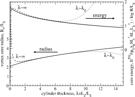
Figure 1: Vortex core radius and energy density, as function of the cylinder thickness. The dotted and dashed lines show approximate analytical expressions, the solid lines are the result of the exact numerical calculation.

Conclusions

Starting with the description of magnetization distributions via complex variable, various simplifying physical approximations for magnetic Hamiltonian were consistently (in the same notations and units) presented and compared with their advantages and deficiencies highlighted. Formulas for the exchange energy of such distributions (10)-(11), provided the vortices and anti-vortices are fully contained inside the particle (which covers many distributions of Ref. [14]), were presented here for the first time. Two simple and explicit analytical approximations for equilibrium vortex core radius and energy in circular cylinder were derived, which, together, cover the whole range of cylinder geometries.

References

- [1] T. Skyrme, A unified field theory of mesons and baryons, Nuclear Physics A. 31 (1962) 556–569. doi:10.1016/0029-5582(62)90775-7.
- [2] A. A. Belavin, A. M. Polyakov, Metastable states of two-dimensional isotropic ferromagnet., ZETP lett. 22 (10) (1975) 245–247, (in Russian).
- [3] W. Doring, Point singularities in micromagnetism, Journal of Applied Physics 39 (2) (1968) 1006–1007. doi:10.1063/1.1656144.
- [4] G. Woo, Pseudoparticle configurations in two-dimensional ferromagnets, Journal of Mathematical Physics 18 (6) (1977) 1264–1266. doi:10.1063/1.523400.
- [5] D. J. Gross, Meron configurations in the two-dimensional o(3) -model, Nuclear Physics B 132 (5) (1978) 439–456. doi:10.1016/0550-3213(78)90470-4.
- [6] K. L. Metlov, Two-dimensional topological solitons in small exchange-dominated cylindrical ferromagnetic particles, arXiv:cond-mat/0012146 (2000).
- [7] J. M. Kosterlitz, D. J. Thouless, Ordering, metastability and phase transitions in two-dimensional systems, Journal of Physics C: Solid State Physics 6 (7) (1973) 1181.
- [8] N. A. Usov, S. E. Peschany, Magnetization curling in a fine cylindrical particle, J. Magn. Magn. Mater. 118 (1993) L290–L294.
- [9] N. A. Usov, S. E. Peschany, Magnetization curling in a thin ferromagnetic cylinder, Fiz. Met. Metal (in Russian) 12 (1994) 13–24.
- [10] T. Shinjo, T. Okuno, R. Hassdorf, K. Shigeto, T. Ono, Magnetic vortex core observation in circular dots of permalloy, Science 289 (2000) 930–932.
- [11] B. Van Waeyenberge, A. Puzic, H. Stoll, K. W. Chou, T. Tyliszczak, R. Hertel, M. Fahnle, H. Bruckl, K. Rott, G. Reiss, I. Neudecker, D. Weiss, C. H. Back, G. Schutz, Magnetic vortex core reversal by excitation with short bursts of an alternating field, Nature 444 (7118) (2006) 461–464. doi:10.1038/nature05240.
- [12] R. Antos, Y. Otani, Simulations of the dynamic switching of vortex chirality in magnetic nanodisks by a uniform field pulse, Phys. Rev. B 80 (2009) 140404. doi:10.1103/PhysRevB.80.140404.
- [13] V. S. Pribiag, I. N. Krivorotov, G. D. Fuchs, P. M. Braganca, O. Ozatay, J. C. Sankey, D. C. Ralph, R. A. Buhrman, Magnetic vortex oscillator driven by d.c. spin-polarized current, Nature Phys. 3 (7) (2007) 498–503.
- [14] K. L. Metlov, Magnetization patterns in ferromagnetic nano-elements as functions of complex variable, Phys. Rev. Lett. 105 (2010) 107201.
- [15] A. Aharoni, Introduction to the theory of ferromagnetism, Oxford University Press, Oxford, 1996.
- [16] T. Bose, S. Trimper, Retardation effects in the landau-lifshitz-gilbert equation, Phys. Rev. B 83 (2011) 134434. doi:10.1103/PhysRevB.83.134434.
- [17] R. V. Kohn, V. V. Slastikov, Another thin-film limit of micromagnetics, Archive for Rational Mechanics and Analysis 178 (2005) 227–245.
- [18] K. Y. Guslienko, K. L. Metlov, Evolution and stability of a magnetic vortex in small cylindrical ferromagnetic particle under applied field., Phys. Rev. B 63 (10) (2001) 100403R.
- [19] K. L. Metlov, K. Y. Guslienko, Stability of magnetic vortex in soft magnetic nano-sized circular cylinder, J. Magn. Magn. Mater. 242–245 (2002) 1015–1017.