Bayesian inference on dependence in multivariate longitudinal data

Abstract

In many applications, it is of interest to assess the dependence structure in multivariate longitudinal data. Discovering such dependence is challenging due to the dimensionality involved. By concatenating the random effects from component models for each response, dependence within and across longitudinal responses can be characterized through a large random effects covariance matrix. Motivated by the common problems in estimating this matrix, especially the off-diagonal elements, we propose a Bayesian approach that relies on shrinkage priors for parameters in a modified Cholesky decomposition. Without adjustment, such priors and previous related approaches are order-dependent and tend to shrink strongly toward an AR-type structure. We propose moment-matching (MM) priors to mitigate such problems. Efficient Gibbs samplers are developed for posterior computation. The methods are illustrated through simulated examples and are applied to a longitudinal epidemiologic study of hormones and oxidative stress.

Key words: Cholesky decomposition, covariance matrix, moment-matching, oxidative stress, random effects, shrinkage prior.

^aWatson Research Center (Yorktown), IBM, Statistical Analysis & Forecasting, Mathematical Sciences Department, NY, 10603
^bDepartment of Statistical Science, Duke University, Durham, NC 27708-0251
^cEunice Kennedy Shriver National Institute of Child Health & Human Development,
National Institutes of Health, Bethesda, MD 20892

1 Introduction

In biomedical applications, there is increasing interest in the analysis of multivariate longitudinal data, with Fieuws et al. (2007) providing a recent review of the literature in this area. When the dependence structure between different responses is not of interest, one can potentially use marginal models for each response. Gray and Brookmeyer (2000) use such an approach to combine inferences about a treatment effect, using generalized estimating equations for model fitting. When the focus is instead on the time-varying relationship between the different longitudinal responses, one can use a multivariate random effects model, which allows correlations between random effects in component models for each response (Shah et al., 1997; Chakraborty et al., 2003, among others). Fieuws and Verbeke (2004) showed that the random effects approach to joint modeling can sometimes produce misleading results if the covariance structure is misspecified.

A well known problem that arises in fitting a joint random effects model to multivariate longitudinal data is the presence of many unknown parameters in the random effects covariance matrix. This makes standard methods for fitting random effects models subject to convergence problems. Even when the covariance matrix can be estimated, the estimate tends to have a large variance and typical methods do not allow for inferences on whether off-diagonal elements of the random effects covariance are non-zero. These issues lead to difficulties in interpretation, which motivated Putter et al. (2008) to develop a latent class modeling approach. In this article, we instead attempt to improve the performance of the joint random effects modeling approach through the use of a Bayesian method with carefully-chosen priors placed on the covariance matrix to favor sparsity.

This article is motivated by data from the BioCycle study, which collected longitudinal measurements of markers of oxidative stress and reproductive hormones over the menstrual cycle (Wactawski-Wende et al., 2009). The goal is to improve understanding of the dynamic relationship between these variables as this relationship has complicated studies in women of reproductive age with adverse health effects attributable to oxidative stress (Schisterman et al., 2010). In this study, fertility monitors were used to time clinic visits and blood draws during two menstrual cycles from 259 women (Howards et al., 2009). Visits were scheduled within each cycle during (1) menstruation, (2) mid follicular phase, (3) late follicular phase, (4) luteinizing hormone (LH) /follicle stimulating hormone (FSH) surge, (5) ovulation, (6) early luteal phase, (7) mid luteal phase and (8) late luteal phase. Serum samples were assayed for hormone levels including estradiol (E2) and oxidative stress levels as measured by F2 Isoprostanes (F2Iso). In this paper, we focus on investigating the relationship between F2Iso, a biomarker of oxidative stress levels, and estradiol (E2). The BioCycle Study provides a unique opportunity to study dependence in hormone and oxidative stress trajectories. Hormonal patterns tend to follow patterns regulated by the hypothalamic-pituitary-ovarian axis, and are strongly correlated from cycle to cycle.

Following common practice for multivariate longitudinal data analysis, we initially consider a linear mixed effects model (Laird and Ware, 1982) for each response. In particular, let $y_{hij}$ denote the measurement of response type $h$ for subject $i$ at visit $j$, with $h=1$ for log-transformed E2 and $h=2$ for log-transformed F2Iso, and $i=1,\ldots,n$, $j=1,\ldots,n_{i}$. Although our methods focus on the bivariate case, they apply directly to general multivariate longitudinal response data. We allow for unequal number and spacing of visits for the different women, assuming the visits are missing at random (MAR) (Rubin, 1976). This assumption is deemed appropriate based on discussions with the study investigators, as it is unlikely that the missing scheduled visits were related to the F2Iso and E2 measurements on the day of the missed visit. Letting ${\bf x}_{hij}$ and ${\bf z}_{hij}$ denote the $p\times 1$ and $q\times 1$ vectors of predictors, we assume

$$y_{hij} = {\bf x}_{hij}^{\prime}\mbox{\boldmath$\beta$}+{\bf z}_{hij}^{\prime}{\bf b}_{hi}+\epsilon_{hij},\quad{\bf b}_{hi}\sim\mbox{N}_{q}({\bf 0},\mbox{\boldmath$\Omega$}),\quad\epsilon_{hij}\sim\mbox{N}(0,\sigma^{2}),$$ (1)

where $\beta$ is a vector of unknown fixed effects parameters, ${\bf b}_{hi}$ is a vector of random effects and is assumed independent of the measurement error $\epsilon_{hij}$, $\Omega$ is the $q\times q$ random effects covariance matrix that reflects the dependence structure within and across responses, and $\sigma^{2}$ is the residual variance.

The joint mixed effects model (1) is flexible in allowing separate fixed and random effects for each response through the appropriate choice of ${\bf x}_{hij}$ and ${\bf z}_{hij}$, while accommodating dependence in the longitudinal trajectories through dependence in the random effects. Such dependence is measured by the off-diagonal elements in the random effects covariance matrix $\Omega$. In the BioCycle study, there is substantial variability in both F2Iso and E2 across the menstrual cycle as shown in Figure 1. Prior substantive knowledge suggests that the trajectories of F2Iso and E2 over the cycle may differ for different women, especially by menopausal status and body fat distribution. Although we expect the patterns to be more similar among women in the BioCycle study who were selected into the study because they were healthy and regularly menstruating, there still exists considerable variability. Hence, when studying certain populations it may not be reasonable a priori to assume a simple parametric model, such as a random intercept model. We instead assume separate fixed and random effect coefficients for each visit. This results in $p=9$ (intercept and coefficients for the eight visits from each woman) and $q=16$ (total number of responses if the woman attended all of her scheduled visits for the two cycles), for a total of $16\times 15/2+9=129$ fixed and random effects parameters to be estimated from the data of only 259 women.

In addition to the well-known problems of estimating a large number of parameters without regularization, frequentist fitting of linear mixed models with large numbers of random effects encounters computational problems in requiring many inversions of a large covariance matrix. The covariance matrix estimate is often ill-conditioned in such cases, with the ratio between the largest and smallest eigenvalues being large. This leads to amplification of numerical errors when the matrix is inverted, resulting in either a lack of convergence or apparent convergence to a poor estimate having substantial bias and high variance. In fact, we first attempted to fit this model using a standard frequentist approach implemented in R 2.10.1 with the lme() function (Pinheiro and Bates., 1996; Lindstrom and Bates, 1982), but failed to obtain convergence for the BioCycle data.

Given these problems, and our interest in inferences on certain off-diagonal elements of the random effects covariance matrix $\Omega$, we instead adopt a Bayesian approach. The typical Bayesian approach to linear mixed effects models (e.g., Zeger and Karim, 1991; Gilks, 1993), either assumes a priori independence among the random effects or chooses an inverse-Wishart prior distribution for the random effects covariance structure. However, since the inverse-Wishart prior incorporates only a single degree of freedom, it is not flexible enough as a shrinkage prior for a high-dimensional covariance matrix. One natural solution is to choose a prior that favors sparsity, shrinking most insignificant elements of the covariance matrix to values close to zero. This can stabilize estimation and improve inferences on significant dynamic correlations.

A variety of the shrinkage priors for $\Omega$ have been proposed in the literature, achieving model flexibility while not sacrificing the positive definite constraint through the use of matrix decompositions. Daniels and Kass (1999) proposed priors that favor shrinkage towards a diagonal structure. Daniels and Pourahmadi (2002) developed alternative priors based on a Cholesky decomposition, giving advantages in interpretation and computation. Smith and Kohn (2002) proposed a parsimonious covariance estimation approach for longitudinal data that avoids explicit specification of random effects. Motivated by the problem of selecting random effects with zero variance, Chen and Dunson (2003) proposed a modified Cholesky decomposition that facilitates choice of conditionally-conjugate priors. Pourahmadi (2007) demonstrated appealing properties of the Chen and Dunson (2003) decomposition in terms of separation of the variance and correlation parameters.

However, we find that posterior computation for the previously proposed sparse shrinkage priors generally does not scale well as the number of random effects increases and there are issues in overly-favoring shrinkage towards AR-type covariance structures. Motivated by the multivariate longitudinal BioCycle data, we propose a new class of heavy-tailed shrinkage priors on the parameters in the Chen and Dunson (2003) decomposition. These priors are robust and introduce substantial computational advantages. It is noted that shrinkage priors under Cholesky-type decomposition have computational advantages but induce order dependence and tend to over-shrink as the locations of the covariance matrix move further off the diagonal. To mitigate this problem, we propose moment-matching priors. Efficient Gibbs samplers are developed for posterior inferences under both priors.

In Section 2, we describe the modified Cholesky decomposition of the covariance matrix and propose new shrinkage priors for the parameters in this decomposition. In Section 3, we describe the order dependence phenomenon and propose the moment-matching priors. Section 4 outlines a simple Gibbs sampling algorithm for posterior computation. Section 5 applies the methods to simulated datasets. Section 6 considers the application to the BioCycle study and Section 7 concludes with a discussion.

2 Shrinkage Priors for Random Effects Covariance Matrices

In order to carry out a Bayesian analysis of model (1), we adopt the modified Cholesky decomposition of the covariance matrix $\Omega$ by Chen and Dunson (2003),

$$\mbox{\boldmath$\Omega$}=\mbox{\boldmath$\Lambda$}\mbox{\boldmath$\Gamma$}\mbox{\boldmath$\Gamma$}^{\prime}\mbox{\boldmath$\Lambda$},$$ (2)

where $\mbox{\boldmath$\Lambda$}=\mbox{diag}(\lambda_{1},\ldots,\lambda_{q})$ is a diagonal matrix with $\lambda_{l}\geq 0$ for $l=1,\ldots,q$, and $\Gamma$ is a $q\times q$ unit lower triangular matrix with $\gamma_{ml}$ in entry ($m,l$). The diagonal elements of $\Lambda$ and the lower triangular elements of $\Gamma$ are vectorized as follows,

$$\mbox{\boldmath$\lambda$}=(\lambda_{1},\ldots,\lambda_{q})^{\prime},\quad\mbox{\boldmath$\gamma$}=(\gamma_{21},\gamma_{31},\gamma_{32},\ldots,\gamma_{q,q-2},\gamma_{q,q-1})^{\prime}.$$

The elements of $\lambda$ are proportional to the standard deviations of the random effects. Setting $\lambda_{l}\approx 0$ is effectively equivalent to excluding the $l$th random effect from the model. By doing so, we move between models of different dimensions, while keeping the covariance matrix of the random effects in each of these models positive definite. The elements of $\gamma$ characterize the correlations between the random effects.

Reparameterizing (1) with the modified Cholesky decomposition, we have

$$y_{hij} = {\bf x}_{hij}^{\prime}\mbox{\boldmath$\beta$}+{\bf z}_{hij}^{\prime}\mbox{\boldmath$\Lambda$}\mbox{\boldmath$\Gamma$}{\bf a}_{hi}+\epsilon_{hij},\quad{\bf a}_{hi}\sim\mbox{N}_{q}({\bf 0},{\bf I}_{q}),\quad\epsilon_{hij}\sim\mbox{N}(0,\sigma^{2}),$$ (3)

where ${\bf I}_{q}$ denotes a $q\times q$ identity matrix. Following Chen and Dunson (2003), we define two vectors

$$u_{hij}=(a_{hil}\lambda_{m}z_{hijm})^{\prime},\quad t_{hij}=\bigg{\{}z_{hijl}\big{(}a_{hil}+\sum_{m=1}^{l-1}a_{him}\gamma_{ml}\big{)}\bigg{\}}^{\prime},\quad 1\leq l<m\leq q.$$

Then (3) can be rewritten as,

$$y_{hij}-{\bf x}_{hij}^{\prime}\mbox{\boldmath$\beta$}-\sum_{l=1}^{q}a_{hil}\lambda_{l}z_{hijl} = u_{hij}^{\prime}\mbox{\boldmath$\gamma$}+\epsilon_{hij},$$ (4)

$$y_{hij}-{\bf x}_{hij}^{\prime}\mbox{\boldmath$\beta$} = t_{hij}^{\prime}\mbox{\boldmath$\lambda$}+\epsilon_{hij}.$$ (5)

Therefore prior distributions for $\Omega$ can be induced through priors on $\mbox{\boldmath$\lambda$},\mbox{\boldmath$\gamma$}$ and all the model parameters can be updated as in the normal linear regression.

We first introduce the priors for the fixed effects (covariates) coefficients $\beta$. When the number of covariates is large, subset-selection is often desirable. In the Bayesian literature, this is usually achieved by introducing a latent variable $J_{l}\in\{0,1\}$ for each covariate that indicates whether it is included in the model, and assuming a spike and slab prior for $\beta_{l}$ conditional on $J_{l}$ (George and McCulloch, 1997; Smith and Kohn, 1996). Let $\mbox{\boldmath$\beta$}^{J}=\{\beta_{l}:J_{l}=1\}$ be the set of coefficients of the selected fixed effects and ${\bf X}^{J}$ be the corresponding covariates matrix. We assume a standard i.i.d. Bernoulli prior for $J_{l}$: $J_{l}\sim\mbox{Bernoulli}(p_{0})$, and express prior ignorance by setting $p_{0}\sim\mbox{beta}(a_{p},b_{p})$. Then, for each of the $\beta_{l}$’s with $J_{l}=0$, we assume the prior to be a point mass at $0$; and for $\mbox{\boldmath$\beta$}^{J}$, we assume a Zellner g-prior (Zellner and Siow, 1980),

$$\mbox{\boldmath$\beta$}^{J}\sim\mbox{N}(0,\sigma^{2}({\bf X}^{J^{T}}{\bf X}^{J})^{-1}/g),\quad g\sim\mbox{G}({1/2},{N/2}),$$

where $\sigma^{2}$ follows a Jeffrey’s prior $\sigma^{2}\propto 1/\sigma^{2}$ is the same $\sigma^{2}$ in model (1), $N=\sum n_{i}$ and $\mbox{G}(a,b)$ denotes a Gamma distribution with mean $a/b$ and variance $a/b^{2}$.

For $\lambda$, we consider another point mass mixture prior similar to that of the $\beta$’s, allowing for random effect selection. Specifically, we assume an i.i.d. zero-inflated half-normal distribution for $\lambda_{l}~{}(l=1,...,q)$,

$$\lambda_{l}|\phi_{l},p_{l}\sim p_{l}\delta_{0}+(1-p_{l})\mbox{N}^{+}(0,\sigma^{2}\phi_{l}^{2}),\quad\phi_{l}^{2}\sim\mbox{IG}(1/2,1/2),$$ (6)

where $\delta_{0}$ is a point mass at 0 and $\mbox{N}^{+}(0,\phi_{l}^{2})$ is the normal distribution $\mbox{N}(0,\phi_{l}^{2})$ truncated to its positive support. When $\lambda_{l}>0$ for all $l$, the decomposition in (2) guarantees that $\Omega$ is positive definite and $\Lambda$ and $\Gamma$ are identifiable. When $\lambda_{l}=0$, elements of the resulting $\Omega$ in the $l$th row and $l$th column are 0. The submatrix of $\Omega$ formed by removing the $l$th row and $l$th column will still be positive definite. Therefore we are able to move between models with different dimensions by removing these rows and columns while still keeping the covariance matrix of the random effects of all these models positive definite. The hyperparameter $p_{l}$ represents the prior probability of $\lambda_{l}=0$ and is set to be $0.5$ to express prior ignorance. The induced marginal prior for $\lambda_{l}$ from (6) is a mixture of a heavy-tailed truncated Cauchy distribution and a point mass at zero.

The parameters of primary interest in this study are the correlations of the random effects, which depend on $\gamma$. Without restriction, the large number of unknown parameters in $\gamma$ relative to the sample size can lead to difficulty in model fitting. We thus consider the following Normal-Exponential-Gamma (NEG) shrinkage prior (Griffin and Brown, 2007):

$$\gamma_{ml}|\psi_{ml}\sim\mbox{N}(0,\sigma^{2}\psi_{ml}),\quad\psi_{ml}\sim\mbox{Exp}({\delta^{2}/2}),\quad\delta^{2}\sim\mbox{G}(c_{0},d_{0}).$$ (7)

The hyperparameters $(c_{0},d_{0})$ control the degree of model sparsity. A larger $c_{0}$ and/or a smaller $d_{0}$ lead more coefficients to be close to zero. The prior has fatter tails and larger variance as $d_{0}$ increases. We set $c_{0}=1$ to introduce more shrinkage and let $d_{0}\sim\mbox{G}(1,1)$ to make the priors more flexible.

3 Moment Matching Prior

As noted in Pourahmadi (2007), a perceived order among the variables is central to the statistical interpretations of the entries of $\Lambda$ and $\Gamma$ as certain prediction variances and moving average coefficients. For longitudinal and functional data there is a natural time-order, while for others, the context may not suggest a natural order. The intrinsic order dependence in shrinkage priors based on Choleskey-type decompositions, including not only Chen and Dunson (2003) but also Daniels and Pourahmadi (2002), favors shrinkage towards an autoregressive-type covariance structure. Such methods can over shrink non-zero covariance not close to the diagonal. This motivated us to develop the following MM prior to mitigate such order dependence problems.

Let $\gamma_{[ml]}$ denote the $m$th and $l$th row of the lower triangular matrix $\Gamma$ and $\mu_{[ml]}$ denote the corresponding prior mean for $\gamma_{[ml]}$,

$$\gamma_{[ml]}=(\gamma_{m1},\ldots,\gamma_{m,m-1},\gamma_{l1},\ldots,\gamma_{l,l-1}),\quad\mu_{[ml]} = (\mu_{m1},\ldots,\mu_{m,m-1},\mu_{l1},\ldots,\mu_{l,l-1}),$$

$$1\leq l<m\leq q.$$

Also denote the correlation matrix corresponding to $\Omega$ by $\rho$. Chen and Dunson (2003) showed that $\rho_{ml}$, the $(m,l)$th entry of $\rho$, is determined solely by $\gamma_{[ml]}$ as follows,

$$\rho_{ml}=h(\gamma_{[ml]})=\frac{\gamma_{ml}+\sum_{r=1}^{l-1}\gamma_{lr}\gamma_{mr}}{\sqrt{(1+\sum_{r=1}^{l-1}\gamma_{lr}^{2})(1+\sum_{r=1}^{m-1}\gamma_{mr}^{2})}}.$$ (8)

This property is crucial to the introduction of the MM prior. Our key idea is to pair-wisely match the first and second prior moments of $\rho$ to those induced from the priors for $\gamma$’s. The first order Taylor expansion of $h(\gamma_{[ml]})$ at the prior mean of $\gamma_{[ml]}$ gives,

$$h(\gamma_{[ml]}) \approx h(\mu_{[ml]})+\nabla h(\mu_{[ml]})^{\prime}(\gamma_{[ml]}-\mu_{[ml]}),$$ (9)

where $\nabla h(\mu_{[ml]})=(\frac{\partial h(\mu_{[ml]})}{\partial\gamma_{m1}},\ldots,\frac{\partial h(\mu_{[ml]})}{\partial\gamma_{m,m-1}},\frac{\partial h(\mu_{[ml]})}{\partial\gamma_{l1}},\ldots,\frac{\partial h(\mu_{[ml]})}{\partial\gamma_{l,l-1}})^{\prime}$. Applying the expectation operator with respect to the prior distribution of $\gamma_{[ml]}$ to (9), we have

$$\mbox{E}(\rho_{ml})=\mbox{E}\{h(\gamma_{[ml]})\}\approx h(\mu_{[ml]})=\frac{\mu_{ml}+\sum_{r=1}^{l-1}\mu_{lr}\mu_{mr}}{\sqrt{(1+\sum_{r=1}^{l-1}\mu_{lr}^{2})(1+\sum_{r=1}^{m-1}\mu_{mr}^{2})}},\quad 1\leq l<m\leq q.$$ (10)

Fixing the values of $\mbox{E}(\rho_{ml})$’s and replacing the approximation by equation (10), we define a system of $q(q-1)/2$ equations for the prior means $\mu_{[ml]}$’s. Similarly, applying the variance operator to (9), we have

$$\mbox{Var}(\rho_{ml})=\mbox{Var}\big{\{}h(\gamma_{[ml]})\big{\}}\approx\nabla h(\mu_{[ml]})^{\prime}\Psi_{\gamma_{[ml]}}\nabla h(\mu_{[ml]}),\quad 1\leq l<m\leq q,$$

where $\Psi_{\gamma_{[ml]}}$ is the prior covariance matrix of $\gamma_{[ml]}$, with the variance of $\gamma_{mk}$ denoted by $\psi_{mk}$ and the covariance between $\gamma_{lj}$ and $\gamma_{mk}$ denoted by $\psi_{lj,mk}$. Rewriting the matrix product in the form of summations and replacing the approximation by the equation above, we have

$$\mbox{Var}(\rho_{ml})=\left\{\begin{array}[]{cll}\sum_{k=1}^{m-1}\psi_{mk}\big{(}\frac{\partial h(\mu_{[ml]})}{\partial\mu_{mk}}\big{)}^{2}+2\sum_{1\leq k<j}^{m-1}\psi_{mk,mj}\frac{\partial h(\mu_{[ml]})}{\partial\mu_{mk}}\frac{\partial h(\mu_{[ml]})}{\partial\mu_{mj}},&\mbox{for}\quad l=1,\\ \mbox{Var}(\rho_{l1})+\mbox{Var}(\rho_{m1})+2\sum_{j=1}^{l-1}\sum_{k=1}^{m-1}\psi_{lj,mk}\frac{\partial h(\mu_{[lj]})}{\partial\mu_{lj}}\frac{\partial h(\mu_{[mk]})}{\partial\mu_{mk}},&\mbox{for}\quad 2\leq l<m\leq q,\end{array}\right.$$ (11)

where

$$\frac{\partial h(\mu_{[ml]})}{\partial\mu_{mk}}=\left\{\begin{array}[]{cl}d_{ml}\big{[}\mu_{lk}(1+\sum_{r=1}^{m-1}\mu_{mr}^{2})-(\mu_{ml}+\sum_{r=1}^{l-1}\mu_{lr}\mu_{mr})\mu_{mk}\big{]},&\mbox{for}\quad k<l<m,\\ d_{mk}\big{[}(1+\sum_{r=1}^{m-1}\mu_{mr}^{2})-\mu_{mk}(\mu_{mk}+\sum_{r=1}^{k-1}\mu_{kr}\mu_{mr})\big{]},&\mbox{for}\quad k=l<m,\\ -d_{ml}\mu_{mk}(\mu_{ml}+\sum_{r=1}^{l-1}\mu_{lr}\mu_{mr}),&\mbox{for}\quad l<k<m,\end{array}\right.$$

with $d_{ml}=(1+\sum_{r=1}^{l-1}\mu_{lr}^{2})^{-1/2}(1+\sum_{r=1}^{m-1}\mu_{mr}^{2})^{-3/2}$. When $\mbox{Var}(\rho_{ml})$’s and $\mbox{E}(\rho_{ml})$’s are pre-fixed, (11) defines a system of $q(q-1)/2$ equations for the prior covariances $\Psi_{\gamma_{[ml]}}$’s.

Lacking prior information on the random effects, it is reasonable to assume that all elements of the correlation matrix $\rho$ have equal mean and variance a priori, leaving the data to adjust for the real correlations. If we assume a common prior mean $u$ and variance $v$ for $\rho$’s, then $(u,v)$ should be in the range $u\in[-1,1]$ and $u\pm 3\sqrt{v}\in[-1,1]$ to satisfy the condition $\rho_{ml}\in[-1,1]$. Solving (10), we have,

$$\mu_{m1}=u\sqrt{\frac{1+(m-2)u}{\big{(}1+(m-1)u\big{)}(1-u)}},\quad\mu_{ml}=\mu_{m1}\sqrt{\frac{1-u}{\big{(}1+(l-2)u\big{)}\big{(}1+(l-1)u\big{)}}}.$$ (12)

The system of equations (11), however, is in general under-identified because the number of unknowns is larger than the number of equations. Under reasonable simplifying assumptions motivated by the form of (8) and interpretations of Pourahmadi (2007), we assume that $\gamma_{m1},\ldots,\gamma_{m,m-1}$ are independent of each other, the $\gamma_{ml}^{\prime}s$ have common variance, and the correlations between $\gamma_{lj}$ and $\gamma_{mk}$ $(l\neq m)$ are equal. Thus, the number of unknowns and equations become the same and unique solutions for $\psi_{m1}$ and $\psi_{m2}$ can be written with the above assumptions for all $m$ by,

$$\psi_{m1} = v/\sum_{k=1}^{m-1}\big{(}\frac{\partial h(\mu_{[ml]})}{\partial\mu_{mk}}\big{)}^{2}$$

$$\psi_{m2} = -v/(2\sum_{j=1}^{l-1}\sum_{k=1}^{m-1}\frac{\partial h(\mu_{[lj]})}{\partial\mu_{lj}}\frac{\partial h(\mu_{[mk]})}{\partial\mu_{mk}}).$$ (13)

Given the means and variances of $\rho$, we can calculate the corresponding means and variances of $\gamma_{ml}$’s through (12) and (13). To test the effectiveness of the transformation, we can generate $\gamma_{ml}^{\prime}s$ 1000 times and obtain the corresponding estimated prior distributions of $\rho$ through (8). To set values for $(u,v)$, we want to both shrink nonsignificant values as much as possible by setting $u$ close to zero and leave out significant values by setting $v$ as large as possible but within the constraint that $u\in[-1,1]$ and $u\pm 3\sqrt{v}\in[-1,1]$. With the above two criteria, to test the effectiveness of the MM priors, we experiment with different values of $(u,v)$, $(0.05,0.1)$, $(0.1,0.09)$, $(0.15,0.08)$, $(0.2,0.07)$ with different dimensions. In all the experiments, order-dependence is clearly avoided as the entries of $\rho$ move further off the diagonal. The prior distributions are still approximately $\mbox{N}(u,v)$. We notice that with $u=0.05$ or 0.1, the resulting elements of the estimated $\rho$ have relatively larger ranges, while as $u$ increases, the range decreases. To achieve more flexibility, we can set weakly-informative priors for $u$ and $v$ as $u\sim\mbox{N}(\mu_{0},\sigma_{0}^{2})1(\mu\in[-1,1])$ and $v\sim\mbox{IG}(c_{0},d_{0})1(u\pm 3\sqrt{v}\in[-1,1])$ respectively. The corresponding priors for $\mu$ and $\Psi$ can then be calculated from model (12) and (13) and some Jacobian computation is needed.

4 Posterior Inferences

The posterior distribution is obtained by combining priors and the likelihood in the usual way. However, direct evaluation of the posterior distribution seems to be difficult. The joint posterior distribution for $\theta=(\mbox{\boldmath$\beta$},\mbox{\boldmath$\lambda$},\mbox{\boldmath$\gamma$},\sigma^{2})$ in model (3) is given by,

$$p(\theta|y)\propto\bigg{[}\prod_{i=1}^{n}\mbox{N}_{q}({\bf{a}}_{i};0,\mbox{I}_{q})\prod_{h}\big{\{}\prod_{j=1}^{n_{i}}\mbox{N}(y_{hij};{\bf{x}}_{hij}^{\prime}\mbox{\boldmath$\beta$}+{\bf{z}}_{hij}^{\prime}\mbox{\boldmath$\Lambda$}\mbox{\boldmath$\Gamma$}{\bf{a}}_{i},\sigma^{2})\big{\}}\bigg{]}p(\sigma^{2})p(\mbox{\boldmath$\beta$},J,g)p(\mbox{\boldmath$\lambda$},\mbox{\boldmath$\gamma$}),$$ (14)

which has a complex form that makes direct sampling infeasible. Therefore we employ the Gibbs sampler (Gelfand and Smith, 1990) by iteratively sampling from the full conditional distributions of each parameter given the other parameters. The details of our Gibbs sampler is given below:

1. Sampling fixed effects parameter $\beta$ through,

   $$p(\mbox{\boldmath$\beta$}^{J}|\cdots) \sim \mbox{N}(\mu_{\mbox{\boldmath$\beta$}^{J}},\Sigma_{\mbox{\boldmath$\beta$}^{J}}),$$

   where $\Sigma_{\mbox{\boldmath$\beta$}^{J}}=\frac{1}{g+1}(\sum_{h,i,j}\frac{1}{\sigma^{2}}x_{hij}^{J}x_{hij}^{J^{\prime}})^{-1}$ and $\mu_{\mbox{\boldmath$\beta$}^{J}}=\Sigma_{\mbox{\boldmath$\beta$}^{J}}\sum_{h,i,j}\frac{1}{\sigma^{2}}x_{hij}^{J}\phi_{hij}$, with $\phi_{hij}=y_{hij}-z_{hij}^{\prime}\mbox{\boldmath$\Lambda$}\mbox{\boldmath$\Gamma$}{\bf a}_{i}$ and $x_{hij}^{J}$ denoting the subvector of $x_{hij}$, $\{x_{hijl}:J_{l}=1\}$.

2. Sampling $g$ through the following conjugate Gamma distribution,

   $$g \sim \mbox{G}\bigg{(}\frac{p_{J}+1}{2},\frac{\mbox{\boldmath$\beta$}^{J^{\prime}}(\sum_{h,i,j}\frac{1}{\sigma^{2}}x_{hij}^{J^{\prime}}x_{hij}^{J})\mbox{\boldmath$\beta$}^{J}+N}{2}\bigg{)},$$

   where $p_{J}=\sum_{l=1}^{p}1(J_{l}=1)$ and $N=\sum_{i}n_{i}$.

3. Updating $J_{l}$ individually, following results from Smith and Kohn (1996), we have

   $$p(J_{l}=1|\cdots) = \frac{1}{1+h_{l}}$$

   with $h_{l}=\frac{1-p_{l}}{p_{l}}(1+\frac{1}{g})^{\frac{1}{2}}\{\frac{S(J_{l}=1)}{S(J_{l}=0)}\}^{\frac{N}{2}}$ and $S(J)=\phi^{\prime}\phi-\frac{1}{1+g}\phi^{\prime}{\bf X}^{J}({\bf X}^{J^{\prime}}{\bf X}^{J})^{-1}{\bf X}^{J^{\prime}}\phi$.

4. Sampling $\lambda_{l}$ individually from a inflated half-normal distribution with $\zeta_{hij}=y_{hij}-x_{hij}^{J^{\prime}}\mbox{\boldmath$\beta$}^{J}$

   $$p(\lambda_{l}|\cdots) = \mbox{ZI-N}^{+}(\hat{p_{l}},\hat{\lambda_{l}},\hat{\sigma_{l}^{2}})$$

   with $\hat{p_{l}}=\frac{p_{l}}{p_{l}+(1-p_{l})\frac{N(0;0,1)}{N(0;\hat{\lambda_{l}},\hat{\sigma_{l}^{2}})}\frac{1-\Phi(0;\hat{\lambda_{l}},\hat{\sigma_{l}^{2}})}{1-\Phi(0;0,1)}}$, $\hat{\lambda_{l}}=\hat{\sigma_{l}^{2}}(\sum_{h,i,j}\frac{1}{\sigma^{2}}t_{hijl}(\zeta_{hij}-\sum_{k\neq l}t_{hijk}\lambda_{k})$ and $\hat{\sigma_{l}^{2}}=(\sum_{h,i,j}\frac{t_{hijl}^{2}}{\sigma^{2}}+1)^{-1}$.

5. Updating $\gamma$ through the following two circumstances,

   1. If the prior is as described in (7), following Park and Casella (2008), we can use blocked Gibbs sampler to update $\gamma$’s and their concentration parameters as following,

      $$\mbox{\boldmath$\gamma$}\sim\mbox{N}(\mu_{\mbox{\boldmath$\gamma$}},\Sigma_{\mbox{\boldmath$\gamma$}}),\quad\frac{1}{\psi_{l}^{2}}\sim\mbox{Inverse-Gaussian}(\sqrt{\frac{\delta^{2}}{\gamma_{ml}^{2}}},\delta^{2}),$$

      $$\delta^{2}\sim\mbox{G}(c_{0}+r,1/(\sum_{m,l}\frac{\gamma_{ml}^{2}}{2}+d_{0})),\quad d_{0}\sim\mbox{G}(1,1+\delta^{2})$$

      with $\mu_{\mbox{\boldmath$\gamma$}}=\Sigma_{\mbox{\boldmath$\gamma$}}\sum_{h,i,j}\frac{1}{\sigma^{2}}u_{hij}w_{hij}$ and $\Sigma_{\mbox{\boldmath$\gamma$}}=(\sum_{h,i,j}\frac{u_{hij}u_{hij}^{\prime}}{\sigma^{2}}+D_{\psi}^{-1})^{-1}$. $D_{\psi}$ is a diagonal matrix with diagonal elements of $\psi_{ml}$.

   2. If the prior is the MM prior, $\gamma$ is updated by,

      $$p(\mbox{\boldmath$\gamma$}|\cdots)\sim\mbox{N}(\hat{\mbox{\boldmath$\gamma$}},\hat{R})$$

      where $\hat{R}=(\sigma^{-2}\sum_{h,i,j}u_{hij}u_{hij}^{T}+\Psi^{-1})^{-1}$ and $\hat{\mbox{\boldmath$\gamma$}}=\hat{R}\{\sigma^{-2}\sum_{h,i,j}u_{hij}(y_{hij}-x_{hij}^{J^{\prime}}\mbox{\boldmath$\beta$}^{J})+\Psi^{-1}\mbox{\boldmath$\mu$}\}$. $\mu$ and $\Psi$ are obtained from the MM priors described in Section 3 and can be updated through the random walk Metropolis-Hastings method if hyperpriors $u$ and $v$ are not fixed.

6. Sampling random effects ${\bf a}_{hi}$ from

   $$p({\bf a}_{hi}|\cdots) \sim \mbox{N}(\mu_{{\bf a}_{hi}},\Sigma_{{\bf a}_{hi}}),$$

   with $\mu_{{\bf a}_{hi}}=\Sigma_{{\bf a}_{hi}}\sum_{j}\frac{1}{\sigma^{2}}\mbox{\boldmath$\Gamma$}^{\prime}\mbox{\boldmath$\Lambda$}\zeta_{hij}$ and $\Sigma_{{\bf a}_{hi}}=(\sum_{j}\frac{1}{\sigma^{2}}\mbox{\boldmath$\Gamma$}^{\prime}\mbox{\boldmath$\Lambda$}z_{hij}z_{hij}^{\prime}\mbox{\boldmath$\Lambda$}\mbox{\boldmath$\Gamma$}+\mbox{I}_{q})^{-1}$.

7. Sampling $\sigma^{2}$ with $\theta_{hij}=y_{hij}-x_{hij}^{J^{\prime}}\mbox{\boldmath$\beta$}^{J}-z_{hij}^{\prime}\mbox{\boldmath$\Lambda$}\mbox{\boldmath$\Gamma$}{\bf a}_{hi}$ by,

   $$p(\sigma^{2}|\cdots)\sim\mbox{Inverse-Gamma}(N/2,\sum_{h,i,j}\theta_{hij}^{2}/2)$$

After discarding the draws from the burn-in period, we can estimate posterior summaries of the model parameters in the usual way from the Gibbs sampler output.

5 Simulations

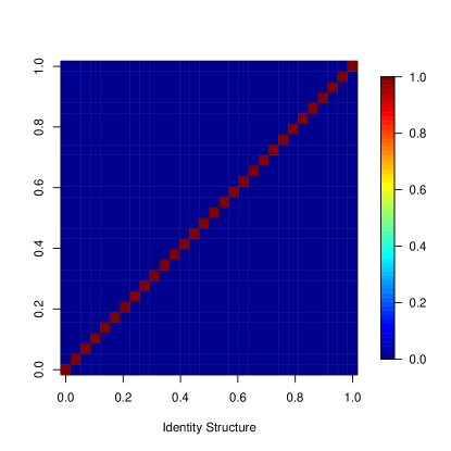
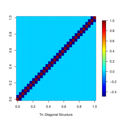
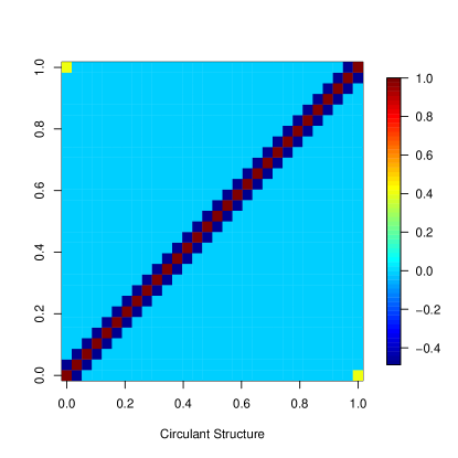
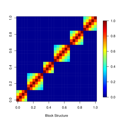
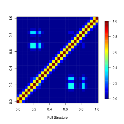
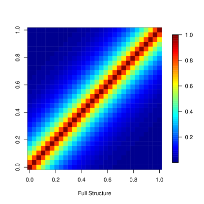
Figure 2: Imageplots for six true covariance matrices

In this section, we examine the performance of the proposed priors on simulated data. Since our primary interest is on the covariance matrix of random effects, we assume there are no fixed effects in the simulations. Data are generated from model (3) with $z_{hij}=\mbox{I}_{q}$. Six representative structures (Figure 2) are considered.

1. The identity structure: $\Omega$ is the identity matrix so all random effects are independent.

2. The tri-diagonal structure: $\Omega$ has unity diagonal entries with the immediate off-diagonal entries being -0.488, corresponding to the covariance matrix of a MA(1) model with decay parameter 0.8. The remaining entries are zero.

3. The circulant structure: similar to the tri-diagonal structure except for an additional pair of entries at $(1,q)$ and $(q,1)$ being set to 0.4.

4. The block diagonal structure: $\Omega$ has six blocks, each viewed as a separate covariance matrix with the entries decreasing from unity at the rate of 0.8 as a function of the distance from the diagonal (i.e., the immediate off-diagonal entries are 0.8 and the next off- diagonals are $0.8^{2}$, and so on). This resembles the situation where the variables are divided into several independent groups and variables within the same group are closely connected.

5. The random structure: $\Omega$ has the diagonals being unity, the immediate off-diagonal entries being 0.4, and some other entries having randomly selected values. We also experiment with other values for the immediate off-diagonal entries. This structure is similar to that in our application, where the data are longitudinal but can have significant points further off the diagonal entries.

6. The full structure: similar to the block diagonal structure, but all variables are now in the same group. Entries decay at the rate of 0.8 as they swing away from the main diagonals, resembling an AR(1) structure.

For each structure, we simulate a data set with 200 subjects, each having 15 visits and 2 outcomes per visit. In total, there are 30 random effects for each subject, i.e., $q=2\times 15=30$.

We first try to estimate the model with functions from the R package nlme, which can fit and compare Gaussian linear and nonlinear mixed-effects models. We can only get estimation when the covariance matrix is diagonal, while all the others fail with an error message “iteration limit reached without convergence”. It seems that the package nlme can only deal with small dimensional data, e.g., q is small. We then try the R package corpcor for comparison with our proposed methods. This package implements a James-Stein-type shrinkage estimator for the covariance matrix, with separate shrinkage for variances and correlations. The details of the method are explained in Schäfer and Strimmer (2005) and Opgen-Rhein and Strimmer (2007). In order to compare the estimated covariance matrix with different methods (the R package corpcor cannot output the covariance matrix for the random effects in the linear mixed effects model), we assume that the residual variance is zero when generating the data. Results with the shrinkage and the MM priors are based on a Gibbs sampler of 20,000 iterations after a burn-in period of 10,000. Estimations are compared based on the squared error loss function,

$$D(\hat{\mbox{\boldmath$\Omega$}},\mbox{\boldmath$\Omega$})=\frac{1}{q^{2}}\big{\{}\sum_{i}\sum_{j}(\hat{\omega}_{ij}-\omega_{ij})^{2}\big{\}}^{1/2}.$$

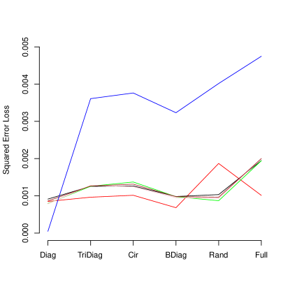
Figure 3: Squared Error Loss for Maximum Likelihood Estimation(blue line), Moment Matching Prior with $(u,v)=(0.05,0.1)$(black line), $(u,v)=(0.1,0.09)$(green line), $(u,v)=(0.15,0.08)$(pink line), $(u,v)=(0.2,0.07)$(brown line) and Shrinkage prior(red line)

where $\omega_{ij}$ is in the $i$th row, $j$th column of $\Omega$ and $\hat{\omega}$ is in the $i$th row, $j$th column of $\hat{\mbox{\boldmath$\Omega$}}$. Figure 3 shows the squared error losses of the estimates from the corpcor, the shrinkage priors and the MM priors. For simplicity, we set fixed values for $(u,v)$ as $(0.05,0.1)$, $(0.1,0.09)$, $(0.15,0.08)$ and $(0.2,0.07)$. Both the shrinkage priors and the MM priors outperform the estimation from the corpcor, except under the diagonal covariance matrix structure. The corpcor performs best when the true underlying covariance matrix is sparse but otherwise tends to over-shrink. When the true underlying covariance structure is diagonal, the shrinkage priors and the MM priors perform equally well. The shrinkage priors have the smallest squared error losses when the underlying covariance structure is tri-diagonal, circulant, block-diagonal and full structure. The MM priors clearly outperform the shrinkage priors when the true underlying covariance structure is random. As expected, the estimates of the shrinkage priors under the random structure tend to over-shrink the parameters as they move further off the diagonal.

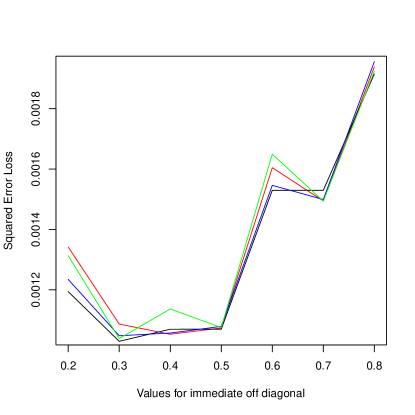
Figure 4: Squared Error Loss for $(u,v)=(0.05,0.1)$(red line), $(u,v)=(0.1,0.09)$(black line), $(u,v)=(0.15,0.08)$(blue line), $(u,v)=(0.2,0.07)$(green line)

To further explore the impact of $(u,v)$ values on the performance of the MM priors, we calculate the MSE for $(u,v)$ values being $(0.05,0.1),(0.1,0.09),(0.15,0.08),(0.2,0.07)$ under different random covariance structures. The difference in MSE from the MM priors among the selected $(u,v)$ values under the above simulation settings are very small. The immediate off-diagonal values are chosen from $\{0.2,0.3,\ldots,0.8\}$ and the randomly selected further-off diagonal values are the same in each test for comparison. MSEs are shown in Figure 4 and the MM priors perform best with $(u,v)=(0.1,0.09)$. Since $(u,v)$ are hyperpriors for the correlation matrix, which will not be affected by the magnitude and scale of the new datasets, we adopt the value (0.1,0.09) in later analyses for simplicity. MSEs are smallest when the immediate off-diagonal value is 0.3 and get larger when the values get larger.

6 Application to the BioCycle Study

Oxygen free radicals have been implicated in spontaneous abortions, infertility in men and women, reduced birth weight, aging, and chronic disease processes, such as cardiovascular disease and cancer. It is thought that estrogen may play an important role in oxidative stress levels in women. However, little is known about the relation between oxidative stress, estrogen levels, and their influence on outcomes, such as likelihood of conception or spontaneous abortions. The primary goals of the BioCycle study are to better understand the intricate relationship between hormone levels and oxidative stress during the menstrual cycle (Schisterman et al., 2010). The BioCycle study enrolled 259 healthy, regularly menstruating premenopausal women for two menstrual cycles. Participants visited the clinic up to 8 times per cycle, at which time blood and urine were collected.

The BioCycle study provides a unique setting for application of the proposed methodology. The data is longitudinal and hormone levels tend to follow predicted patterns across the menstrual cycle due to the complex feedback mechanisms which regulate hormonal levels through the hypothalamic-pituitary-ovary axis. Further, hormone levels during specific phases tend to be correlated from cycle to cycle.

The responses are transformed to a log scale to make the normal assumption more reliable and the predictors are standardized by subtracting the mean and dividing by the standard deviation. Responses of F2Iso and E2 from the first 20 subjects are shown in Figure 1. We can see certain common trends over visits across the women, but more strikingly each individual has her own diversity which makes the plots more variable. Linear mixed-effects models can accommodate such differences and analyze the longitudinal dependences among two types of responses varying over visits through the covariance matrix. Specifically, $y_{hij}$ is the response for type $h$ ($h=1,2$) of subject $i$ ($i=1,\ldots,259$) at visit $j$ ($j=1,\ldots,8$ for the 8 visits). Let $x_{1ij}=(1,x_{i11},x_{i12},x_{i13},x_{i14},0,0,0,0)_{9\times 1}^{{}^{\prime}}$ and $x_{2ij}=(1,0,0,0,0,x_{i21},x_{i22},x_{i23},x_{i24})_{9\times 1}^{{}^{\prime}}$ be the fixed predictors of response $h=1$ and $h=2$, respectively, for subject $i$ at visit $j$. Let $z_{1ij}=(\underbrace{0,\ldots,1_{1ij},\ldots,0}_{8\times 1},\underbrace{0,\ldots,0}_{8\times 1})_{16\times 1}^{{}^{\prime}}$ and $z_{2ij}=(\underbrace{0,\ldots,0}_{8\times 1},\underbrace{0,\ldots,1_{2ij},\ldots,0}_{8\times 1})_{16\times 1}^{{}^{\prime}}$ stand for the random predictors of response $h$ for subject $i$ at visit $j$, where

$$1_{hij}=\left\{\begin{array}[]{lc}1,&\mbox{subject $i$ showed up at visit $j$ for response $h$},\\ \,0,&\mbox{otherwise}.\par\end{array}\right.$$

We attempt to fit model (1) with the lme() function in R 2.10.1 but failed, because the estimates do not converge. We first estimate the covariance structure with the shrinkage priors given the data collected longitudinally. In order to capture the possible sporadic significant signals, we also estimate model (1) with the MM priors with $(u,v)=(0.1,0.09)$. The Raftery and Lewis diagnostic (Raftery and Lewis, 1995) is used to estimate the number of MCMC samples needed for a small Monte Carlo error in estimating the 95% credible intervals. The required sample size can be different for each parameter and 20,000 iterations are found to be enough for all parameters. Convergence diagnostics, such as trace plots and Geweke’s convergence diagnostic for randomly selected off-diagonal elements of the covariance matrix are performed on some selected elements. No signs of adverse mixing is found. All results are based on 50,000 Gibbs sampling iterations after a burn-in period of 20,000.

Figures 5 and 6 display the estimated correlation structures for both within and across responses for the shrinkage and the MM priors respectively. The left panels are the estimated correlation matrices between the two responses and the right panels are the zoomed-in cross correlation structures among the two responses. The left upper 8 by 8 matrix (with the 8 responses from the cycles) is the correlation matrix for response E2 across the cycle. The right lower 8 by 8 matrix is the correlation matrix for the eight F2Iso responses across the cycle. For example, the (2,3)rd cell is the correlation between the second visit and the third visit of response E2; the (10,11)th cell is the correlation between the second visit and the third visit of response F2Iso. The upper right (or the lower left) 8 by 8 matrix is the cross correlation among responses of E2 and F2Iso across the two cycles. For example, the (1,9)th cell is the correlation between the first visit of E2 and the first visit of F2Iso.

Estimated correlation structures through the MM priors help us have a better understanding of the relation between estrogen levels and F2 Isoprostanes during the menstrual cycle: finding more visits with stronger correlations between the two responses. The analysis shows that the correlations appear to differ slightly across the menstrual cycle, with the cross-correlations being low in general. Further, the 5th visit for F2Iso is much less correlated than the others. This could be due to the fact that the mean values of F2Iso tend to be lowest at this point during the cycle (around ovulation when estrogen levels are high), but otherwise are not varying as much at the other visits. Estimates from the shrinkage priors fail to pick up most of the stronger correlations between visits.

7 Discussion

This article has proposed two new methods for Bayesian model selection of fixed and random effects in continuous models. Our approaches rely on shrinkage priors and MM priors to the setting of variable selection of multivariate, correlated random effects with large dimension. Clear advantages over earlier approaches include robustness, efficiency of posterior computation and overcoming the order dependence problem.

Our proposed approach is advantageous in that fixed and random effects are selected simultaneously. In particular, the prior and computational algorithm represent a useful alternative to approaches that rely on inverse-Wishart priors for variance components. There is an increasing realization that inverse-Wishart priors are a poor choice, particularly when limited prior information is available. Although we have focused on LMEs of the Laird and Ware (1982) type, it is straightforward to adapt our methods to a broader class of linear mixed models, accommodating varying coefficient models, spatially correlated data, and other applications.

8 Acknowledgement

This work was supported in part by the Intramural Research Program of the Eunice Kennedy Shriver National Institute of Child Health and Human Development, National Institutes of Health.

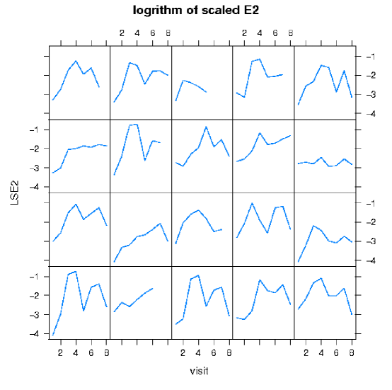
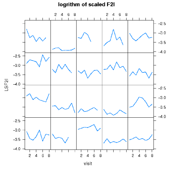
Figure 1: The first $20$ subjects in the data set. Responses LSE2 (logarithm of scaled E2) and LSF2I (logarithm of scaled F2Iso) are shown over visits 1-8.

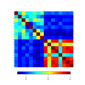
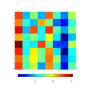
Figure 5: Estimated covariance matrix between log(E2) and log(F2Iso) and the zoomed in cross covariance structure through Moment Matching prior

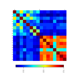
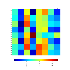
Figure 6: Estimated covariance matrix between log(E2) and log(F2Iso) and the zoomed in cross covariance structure by the shrinkage prior

References

- Chakraborty et al. (2003) Chakraborty, S., K nzli, S., Thiele, L., Herkersdorf, A., and Sagmeister, P. “Performance Evaluation of Network Processor Architectures: Combining Simulation with Analytical Estimation.” Computer Networks, 41:2003 (2003).
- Chen and Dunson (2003) Chen, Z. and Dunson, D. B. “Random effects selection in linear mixed models.” Biometrics, 59:762–769 (2003).
- Daniels and Kass (1999) Daniels, M. and Kass, R. “Nonconjugate Bayesian Estimation of Covariance matrices and its use in hierarchical models.” Journal of the American Statistical Association, 91:198–210 (1999).
- Daniels and Pourahmadi (2002) Daniels, M. and Pourahmadi, M. “Bayesian analysis of covariance matrices and dynamic models for longitudinal data.” Biometrika, 89:553–566 (2002).
- Fieuws and Verbeke (2004) Fieuws, S. and Verbeke, G. “Joint modelling of multivariate longitudinal profiles: pitfalls of the random-effects approach.” Statistics in Medicine, 23:3093 104 (2004).
- Fieuws et al. (2007) Fieuws, S., Verbeke, G., and Molenberghs, G. “Random-effects models for multivariate repeated measures.” Statistical Methods in Medical Research, 16(5):387–397 (2007).
- Gelfand and Smith (1990) Gelfand, A. E. and Smith, A. F. M. “Sampling-based approaches to calculating marginal densities.” Journal of the American Statistical Association, 85:398–409 (1990).
- George and McCulloch (1997) George, E. I. and McCulloch, R. E. “Approaches for Bayesian Variable Selection.” Statistica Sinica, 7:339–373 (1997).
- Gilks (1993) Gilks, W. R. “Modeling complexity: Applications of Gibbs sampling in medicine.” Journal of the Royal Statistical Society, Series B, 55:39–52 (1993).
- Gray and Brookmeyer (2000) Gray, S. and Brookmeyer, R. “Multidimensional longitudinal data: estimating a treatment effect from continuous, discrete, or time-to-event.” Journal of the American Statistical Association, 95(450):396–406 (2000).
- Griffin and Brown (2007) Griffin, J. and Brown, P. “Bayesian adaptive lassos with non-convex penalization.” Tech. Rep. No. 07-02, University of Warwick. (2007).
- Howards et al. (2009) Howards, P., Schisterman, E., Wactawski-Wende, J., Reschke, J., Frazer, A., and Hovey, K. “Timing clinic visits to phases of the menstrual cycle by using a fertility monitor: the BioCycle Study.” American Journal of Epidemiol, 169 (2009).
- Laird and Ware (1982) Laird, N. M. and Ware, J. “Random-Effects Models for Longitudinal Data.” Biometrics, 38:963–974 (1982).
- Lindstrom and Bates (1982) Lindstrom, M. and Bates, D. “Newton-Raphson and EM Algorithms for Linear Mixed-Effects Models for Repeated-Measures Data.” Journal of the American Statistical Association, 83:1014–1022 (1982).
- Opgen-Rhein and Strimmer (2007) Opgen-Rhein, R. and Strimmer, K. “Accurate ranking of differentially expressed genes by a distribution-free shrinkage approach.” Statistical Applicaitons in Genetics and Molecular Biology, 6 (2007).
- Park and Casella (2008) Park, T. and Casella, G. “The Bayesian Lasso.” Journal of the American Statistical Association, 103(482):681–686 (2008).
- Pinheiro and Bates. (1996) Pinheiro, J. and Bates., D. “Unconstrained Parametrizations for Variance-Covariance Matrices.” Statistics and Computing, 6:289–296 (1996).
- Pourahmadi (2007) Pourahmadi, M. “Cholesky Decompositions and Estimation of A Covariance Matrix: Orthogonality of Variance CCorrelation Parameters.” Biometrica, 94:1006–1013 (2007).
- Putter et al. (2008) Putter, H., Vos, T., de Haes, H., and van Houwelingen, H. “Joint analysis of multiple longitudinal outcomes: Application of a latent class model.” Statistics in Medicine, 27:6228 – 6249 (2008).
- Raftery and Lewis (1995) Raftery, A. and Lewis, S. “The number of iterations, convergence diagnostics and generic Metropolis algorithms.” In Practical Markov Chain Monte Carlo (1995).
- Rubin (1976) Rubin, D. “Inference and missing data.” Biometrika, 63 (1976).
- Schäfer and Strimmer (2005) Schäfer, J. and Strimmer, K. “A shrinkage approach to large-scale covariance matrix estimation and implications for functional genomics.” Statistical Applicaitons in Genetics and Molecular Biology, 4 (2005).
- Schisterman et al. (2010) Schisterman, E., Gaskins, A., Mumford, S., Browne, R., Yeung, E., Trevisan, M., Hediger, M., Zhang, C., Perkins, N., Hovey, K., Wactawski-Wende, J., and Group., B. S. “Influence of endogenous reproductive hormones on F2-isoprostane levels in premenopausal women: the BioCycle Study.” American Journal of Epidemiol, 172 (2010).
- Shah et al. (1997) Shah, A., Laird, N., and Schoenfeld, D. “A random-effects model for multiple characteristics with possibly missing data.” Journal of the American Statistical Association, 92(438):775–779 (1997).
- Smith and Kohn (1996) Smith, M. and Kohn, R. “Nonparametric regression using Bayesian variable selection.” Journal of Econometrics, 75:317–343 (1996).
- Smith and Kohn (2002) —. “Parsimonious Covariance Matrix Estimation for Longitudinal Data.” Journal of the American Statistical Association, 97:1141 (2002).
- Wactawski-Wende et al. (2009) Wactawski-Wende, J., Schisterman, E., Hovey, K., Howards, P., Browne, R., Hediger, M., Liu, A., and Trevisan, M. “BioCycle study: design of the longitudinal of the oxidative stress and hormone variation during the menstrual cycle.” Paediatr Perinat Epidemiol, 23 (2009).
- Zeger and Karim (1991) Zeger, S. and Karim, M. “Generalized linear models with random effects: A Gibbs sampling approach.” Journal of the American Statistical Association, 6:79–86 (1991).
- Zellner and Siow (1980) Zellner, A. and Siow, A. “Posterior odds ratios for selected regression hypotheses.” In Bayesian Statistics: Proceedings of the First International Meeting held in Valencia (Spain) (1980).